Assessing Essential Qualities of Urban Space with Emotional and Visual Data Based on GIS Technique

1. Introduction

Urban spaces are closely related to the way people live and work in cities [1,2,3]. Since the Industrial Revolution, people’s approaches to production and lifestyles have further encroached on all aspects of the traditional urban space; thus creating the so called “lost space” [4]. On one hand, people spend more time and money on meaningless commuting [5], which contributes to environmental deterioration and consumes energy [6]; on the other hand, urban space has gradually become occupied by motor traffic—and urban life has been relegated to the sides of the roads [7]. Since the 1960s, scholars have paid more attention to optimizing urban spaces and promoting outdoor activities [8,9,10,11].

In previous studies, measures of urban space and form using computational methods began to be correlated to certain human behaviors. For example, Hillier & Iida showed that centrality measures of the street network (which are based on the geometry of the open spaces generated by the shape and arrangement of buildings) have a significant impact on movement patterns [12], which, in turn, have a significant impact on the use of public space (given that commercial uses are generally located at more frequented locations) [13]. Human cognitive responses to urban space and form are closely related to people’s behaviors. Among the various factors that affect the perceived quality of urban space, vision is extremely important. According to cognitive science, external information acquired by human beings is strongly correlated with vision [14]. Some studies have focused on visual responses to spatial attributes such as openness [15], orientation [16,17], and shape complexity [18], to study how people perceive the built environment as these spatial attributes vary [19,20]. However, the limitations of effective analysis methods make it difficult to objectively determine how the spatial attributes of an urban space affect user’s subjective experiences [21]. Although questionnaire surveys are useful to a certain extent, measurement accuracy could be increased by using the innovative information approaches that have emerged in the era of big data. In recent years, along with the development of information technology, relevant computer-aided methods have been gradually introduced into the fields of urban planning and design [22,23,24]. Some novel methods aimed at understanding how people perceive cities have been tested, such as extracting semantics from locations using photo tags from Flickr [25] and gauging crowd emotion and its spatio-temporal distribution from Twitter data [26,27]. Crowdsourcing physiological conditions by combining data from technical sensors and human sensors could also extend the collection of emotional information in urban studies [28]. Such methods are convenient for comprehensively analyzing urban spatial environments for determining the correlations between various spatial attributes and peoples’ behavior and for evaluating and optimizing design schemes.

This paper starts from the perspective of a city pedestrian and then evaluates collected field data concerning the pedestrians’ emotions. By integrating information techniques and regression models, this study explores how urban spaces affect the emotions of pedestrians at the micro-scale, explores the correlative coupling between urban spatial attributes and people’s emotions, constitutes an effective evaluation method for urban spatial environments, predicts the potential influence of changes, and provides suggestions for improving the rationality and effectiveness of urban designs to better serve urban lifestyles. The goal of this paper is to share our experience of using information technology to assess built environments. The described methodology provides a tool that can improve conventional methods by which urban design professionals evaluate urban spaces. Figure 1 presents the workflow of our research framework and analysis approaches.

2. State of the Art

Based on progress in neuroscience over the past decade, a separate research stream has emerged that aims to obtain insights for the field of architectural design through knowledge and techniques from neuroscience [29]. Important study subjects in this field are the effects of the form and function of architectural environments on human health and wayfinding strategies. Such study has relied largely on virtual environments because such environments make it possible to carefully control the studied parameters. However, because it is unclear how the virtual environment parameters correlate with real space—for example with regard to the incorrect estimation of distances and angles [30]—we decide to conduct this study in a real environment.

In this study, the model we use for measuring emotions is based on the concept of cognitive appraisal, which categorizes a relatively complex set of secondary emotions [31]. Secondary emotions are those that have a major cognitive component and are determined by both their level of arousal (low to high) and their valence (pleasant to unpleasant). Figure 2 shows a model of how various secondary emotions can be located inside a coordinate system.

Hogertz collected emotional data from urban pedestrians (n = 31) in Lisbon using Smartbands and GPS tracking [32] and analyzed the indicated emotional responses compared to the retrospective emotional states of the subjects by visual inspection. He concluded that “specific emotional significance can be measured reliably by recording a person’s EDA (electrodermal activity) variations while walking.” Most importantly, Hogertz found a relationship between people’s negative emotional responses and certain locations.

A further analysis was conducted in the main promenades of Alexandria, where individual stress reactions (n = 7) were identified using a promising workflow [33] in which combined datasets from a GPS tracker, camera, and Smartband, were used to identify subjects’ stress phases over the routes and then extract movie snippets of the relevant sections. To visualize the results, all the individual stress points were aggregated into a heat map that showed the stress hotspots. In addition, individual stress locations were combined into a point density analysis.

In another study, neural imaging using electroencephalograph (EEG) signals was employed to map human responses to spaces [34]. The authors describe an experiment where participants’ affective (emotional) states were measured while the participants moved through open spaces in Edinburgh. The authors used a lightweight, high performance laptop, wireless EEG sensors, and a GPS unit. The collected data were analyzed by mapping them to the defined path in terms of excitement and frustration levels. The study showed the aggregation of excitement levels for three participants.

All these studies used measured emotional responses to show that locations exist in the urban realm that elicit significant emotional responses. However, none of the studies have investigated whether a given individual’s perceptions of urban spaces correlates with the perceptions of other individuals. In other words, they did not ascertain whether certain spatial configurations have a generalizable effect on human emotions. Additionally, none of the studies described above have investigated whether a relationship exists between people’s emotion and isovist field parameters. In preliminary studies we analyzed this relationship using surveys to investigate the effect of urban form on people’s environmental appraisals of streetscapes. We also introduced a geostatistical method for studying the relationships between urban pedestrians’ emotional responses and urban spaces. In this paper, we investigate the effect of additional spatial features on peoples’ spatial perceptions—including the indicators of building texture and shape, isovist parameters, visual entropy, and visual fractals.

3. Emotion Data Collection

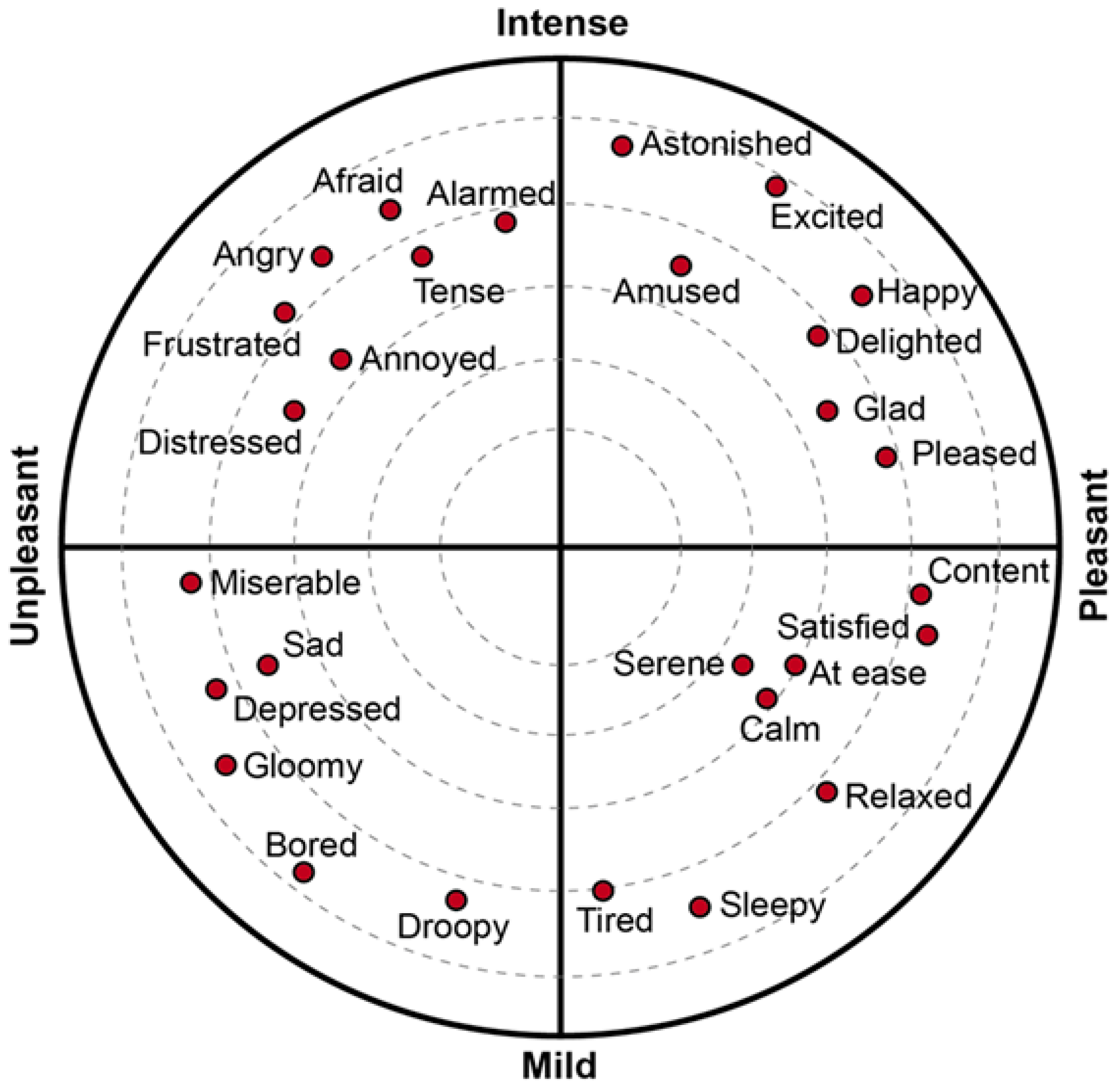
3.1. Physiological Basis

According to research in developmental psychology, normal infants begin to show some common emotional characteristics (such as interest, surprise, joy, anger and fear) when they are between two and a half months and six months old. These inborn emotions are called “primitive emotions” or “primary emotions”, and they have both cross-cultural and cross-regional characteristics [35,36]. Thus, they can be understood by people from different nations, regions and countries. When the infants reach approximately two years of age, depending on their environment, these emotions gradually develop into a wide variety of complex secondary emotions such as embarrassment, shyness, guilt, envy and pride, among others. These emotions are called “self-conscious emotions,” and they reflect people’s major psychological tendencies. The major characteristics of emotions can be described by the model of secondary emotions. In this model (Figure 2), the horizontal axis represents valence. The right side of the horizontal axis shows positive emotions; the left side shows negative emotions. The vertical axis represents arousal, which refers to the individual’s neurological and physiological activation level as stimulated by the external environment. In Figure 2, arousal intensity gradually increases from the bottom to the top.

3.2. Preparation of Experiment

The wristband sensor (Smartband), developed by Bodymonitor [37,38,39], is used in this experiment as a micro-portable vital sign monitor. Through its built-in metal electrode, the Smartband can record a subject’s skin conductivity and temperature, allowing later processing to analyze and judge the wearer’s emotions through the collected data. The device is lightweight, and people can wear it comfortably, thus avoiding any negative psychological impact from the equipment during the experiment. When combined with data collected by a portable GPS tracker, the emotion data recorded by the Smart Band can be aligned with the wearer’s location. Because the temporal resolution of the GPS sensors employed in this experiment is 5 s and that of the Smart Band is 1 s, the accumulated data from the Smart Band is matched with the GPS data every 5 s to form a basic unit.

To ensure that the participants were not familiar with the experiment site, we selected the Oerlikon District, a region approximately 6 km away from downtown Zurich, Switzerland. The route the participants travelled is approximately 2.2 km long, starting from Max Bill Square and ending at the Oerlikon Station Square. This route is occupied by businesses with mixed functions, residences and commerce, all of which have rich urban spatial forms, and included a newly built office area, a quiet residential area and a relatively busier local center. Thirty participants (13 male, 17 female, mean age = 25, SD of age = 2.5) were involved in the experiment, which took place on sunny days from 14 October to 22 October 2013. The experimental route and a map were distributed to the subjects in advance. Subjects were required to complete the entire route on foot and to take photos of places they deemed important for the record. Emotion data were collected by the Smartband. The raw data were initially processed into two groups that respectively represented positive (1478 points) and negative (994 points) emotions. The Bodymonitor company processed and analyzed the raw data collected by the Smartband (for evidence concerning the validity of the Smartband data see the Bodymonitor website [38,39]), but the details of the company’s method are not explicitly published for commercial reasons. When the experiment was over, the emotion data were geospatially projected to OpenStreetMap (OSM) and imported to ArcGIS as point features.

3.3. Emotion Data Preprocessing

The factors that affect the emotions of subjects can be roughly divided into two classes: Class 1 refers to spatial factors at specific locations that are comparatively less affected by time and other random factors; and Class 2 refers to random factors, non-spatially influenced factors, and temporal factors such as activities. Because the subjects were tested at different times, there was no direct mutual interference between subjects; therefore, we can assume that the emotional data measurements were comparatively independent. Consequently, we can take advantage of spatial clustering analysis (SCA) to strengthen the emotional features caused by spatial factors and reduce the interference from random factors. The null hypothesis of SCA specifies that factors are randomly distributed. At the set confidence level (5%), a statistic such as the p-value is required to judge whether the null hypothesis is rejected or not. When the null hypothesis is rejected, the factor’s location and value have a very high spatial correlation. Therefore, we can conclude that subjects commonly possess similar emotional intensities in this location and, then, judge the degree of arousal through the z-score.

Because the SCA is significantly affected by the area used for analysis, it requires an incremental auto-correlation spatial analysis tool for which several threshold values must be set to conduct the test and inspect the z-score of the model. High z-scores mean that a spatial cluster feature is more dominant under this threshold value. An analysis showed that the threshold values of the P collection and the N collection resulted in the most dominant cluster features at 23.5 m and 11 m, respectively. Using the Getis-Ord General G statistic [40], we performed spatial cluster analyses on the two sets of objects. The Getis-Ord General G formula is as follows [41]:

$$\mathrm{G}=\frac{{\displaystyle \sum _{i=1}^n{\displaystyle \sum _{j=1}^n{w}_{ij}{x}_i{x}_j}}}{{\displaystyle \sum _{i=1}^n{\displaystyle \sum _{j=1}^n{x}_i{x}_j}}},\forall j\ne i,$$

(1)

where w_ij is the spatial weight between i and j in all n objects; and x_i and x_j characterize the magnitude of events i and j.

The resulting z-scores of the Getis-Ord General G statistic for the P collection and the N collection were 2.87 and 1.96, respectively. The probabilities that the two sets of objects form a random distribution are both less than 5%; thus, it can be concluded that the quite dominant high-value cluster feature performs at a 95% confidence level. The SCA shows that subjects’ emotion data obviously possess both common characteristics and conformity.

Although the two sets of data are consistent overall, the distribution of arousal does not follow an identifiable pattern. Some obvious high-value points tend to be affected by random factors and may not possess dominant statistical significance. Consequently, determining specific locations that produce universal influence on the subject’s emotions—namely, the effective sampling points (ESP)—is important to further analyze the spatial attributes resulting in such an emotional discrepancy. Using the Getis-Ord Gi* statistic [42], the formulas of the Gi* statistic and the z-value are as follows:

$${\mathrm{G}}_{\mathrm{i}}*=\frac{{\displaystyle \sum _{j=1}^n{w}_{ij}{x}_j}}{{\displaystyle \sum _{j=1}^n{x}_j}}$$

(2)

$$\mathrm{Z}({\mathrm{G}}_{\mathrm{i}}*)=\frac{{\displaystyle \sum _{j=1}^n{w}_{ij}{x}_j-\overline{x}{\displaystyle \sum _{j=1}^n{w_{ij}}^2}}}{s\sqrt{\frac{n{\displaystyle \sum _{j=1}^n{w_{ij}}^2-{\left({\displaystyle \sum _{j=1}^n{w}_{ij}}\right)}^2}}{n-1}}}.$$

(3)

Under the threshold values of 23.5 m and 11 m, hot-spot analysis on the points of the P and N collections can be conducted separately. For each point feature, this method sums the values of the center feature and adjacent features within the threshold value and compares the results with the sum of all the features in the system. The z-score allows statistical evaluation of the cluster regions with high and low values and their significance levels. Point clusters with high or low values form the set of effective sampling points for further analysis, as shown in Figure 3, where the red zones represent the high-value clusters and the dark blue zones represent the low-value clusters. Based on subjects’ ID numbers, these data belong to different examinees, which indicates that some subjects exhibit similar emotional features at these sampling points. The analysis resulted in extracting 348 effective sampling points, of which 254 samples represented positive emotions that were roughly distributed across 11 locations, and 94 samples represented negative emotions that were roughly distributed across 9 locations.

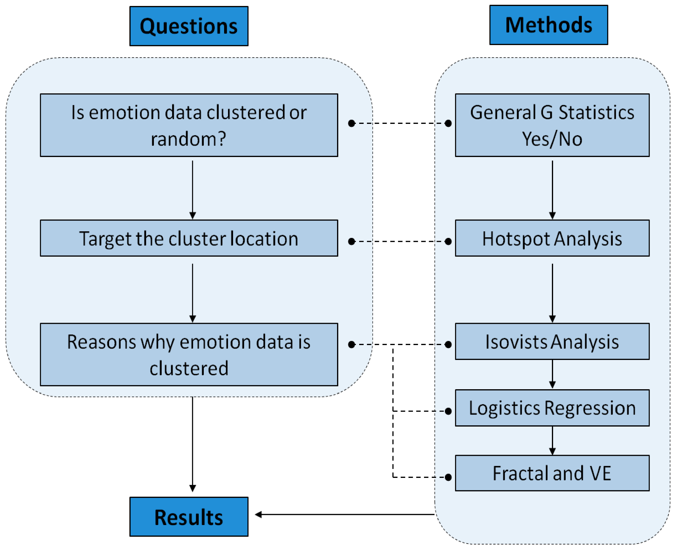
4. Spatial Analysis

Determining the locations that dominantly influenced the emotional characteristics of subjects is fundamental for further analyzing the potential role of urban spatial attributes. To refine the problem, the statistical analysis was roughly carried out in three steps. First, by generating isovists at the ESPs, we extracted the architectural texture within the isovist scope and obtained basic data on the external spatial attributes of the surrounding architecture. Second, we calculated statistics using the isovist parameters based on the ESPs to judge the overall influence of these parameters on subject valences and to establish a regression model for each isovist parameter and valence. Third, we recorded the urban scenery observed by subjects while walking the route by taking photos and comprehensively applying visual entropy and visual fractal dimensions to analyze the spatial attributes represented in these photos and to explore their potential possibilities affecting the valence.

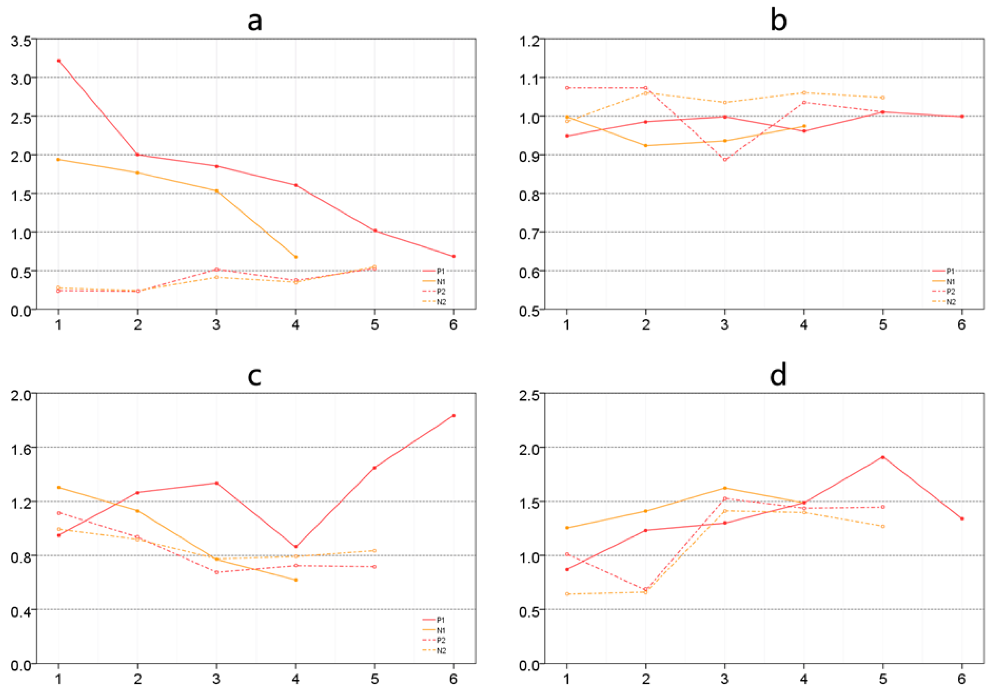
4.1. Influence from Building Texture

The isovist concept has been used for spatial analysis since 1979 [43,44]. The principle is to abstract space into a collection of countless viewpoints, among which the isovist is simplified as a sub-collection mutually and directly viewed between these viewpoints. On this basis, the attributes of an isovist are defined through a series of geometric parameters; then, spatial mapping is further conducted to form an isovist field covering the entire research area. Isovist can be studied from both 2 and 3 dimensional aspects. In this research, we would only limit it to the 2D aspect.

Based on the P collection (11 sets) and N collection (9 sets) of the ESPs identified along the experiment route, we set the isovist radius threshold to 200 m and generated isovist boundaries in ArcGIS for all the sets of sampling points (Figure 4). Then, we extracted the building footprints within those boundaries and calculated the shape index, including the mean area, area dispersion, degree of fragmentation and average distance between buildings. Equation (4) shows the calculation used for area dispersion and Equation (5) shows the calculation for the degree of fragmentation. All the shape indices were normalized by dividing them by the mean value to allow non-dimensional conversion and statistical analysis (

Table 1. Normalized index of building texture.

Sampling Group	Mean Area	Area Dispersion	Average Distance	Degree of Fragmentation
P collection (S1)	1.728	1.356	1.283	0.984
N collection (S1)	1.478	1.443	0.955	0.958
P collection (S2)	0.378	1.220	0.834	1.016
N collection (S2)	0.366	1.076	0.863	1.038

).

$$\mathrm{CoV}\_\mathrm{Area}=\frac{\frac{{\displaystyle \sum \sqrt{\left(S_i^2-\overline{S^2}\right)}}}{\left(N-1\right)}}{\overline{S}}$$

(4)

$$\mathrm{SI}=1-\frac{4\sqrt{S_i}}{P}$$

(5)

Here, S_i refers to the areas of all the architectural outlines within the isovist, $\overline{S}$ refers to the average area of an architectural outline, N refers to the number of architectures, and P refers to the overall length of an architectural outline.

A railway divides the research area into two sites—an eastern portion and a western portion (S1 and S2); therefore, we analyzed the shape index of the two sites under circumstances of different valences (Figure 5). In S1, the shape index of the building footprints corresponding to sites of different valences is noticeably different compared to the shape index in S2. For example, when subjects exhibit positive emotions, the building footprints within the isovist in S1 tends to be larger with a comparatively small deviation. This is possibly due to the influence of building scale; the average center-to-center spacing is large between the buildings in S1. Moreover, the building texture fragmentation is higher in S1, reflecting a complicated overall outline and a spatial hierarchy within this area. In S2, under the circumstance of different valences, the shape indices other than fragmentation have collinear characteristics, indicating that the factors affecting the subject’s emotions may not be triggered by these shape indices in S2. Therefore, in S2, it can be speculated that the influence of urban form on emotions may have a comparatively secondary status.

An independent sample t-test was further applied to analyze the shape index of the P collection and the N collection. The results showed that no indicators are significant (p > 0.05) at a confidence level of 95%. Therefore, although we can compare differences in architectural texture using the shape indices among a few ESPs, it is difficult to predict other locations. Consequently, other spatial attributes (such as isovist parameters) must be employed to conduct a deep analysis and to explore other, more dominant spatial influential factors.

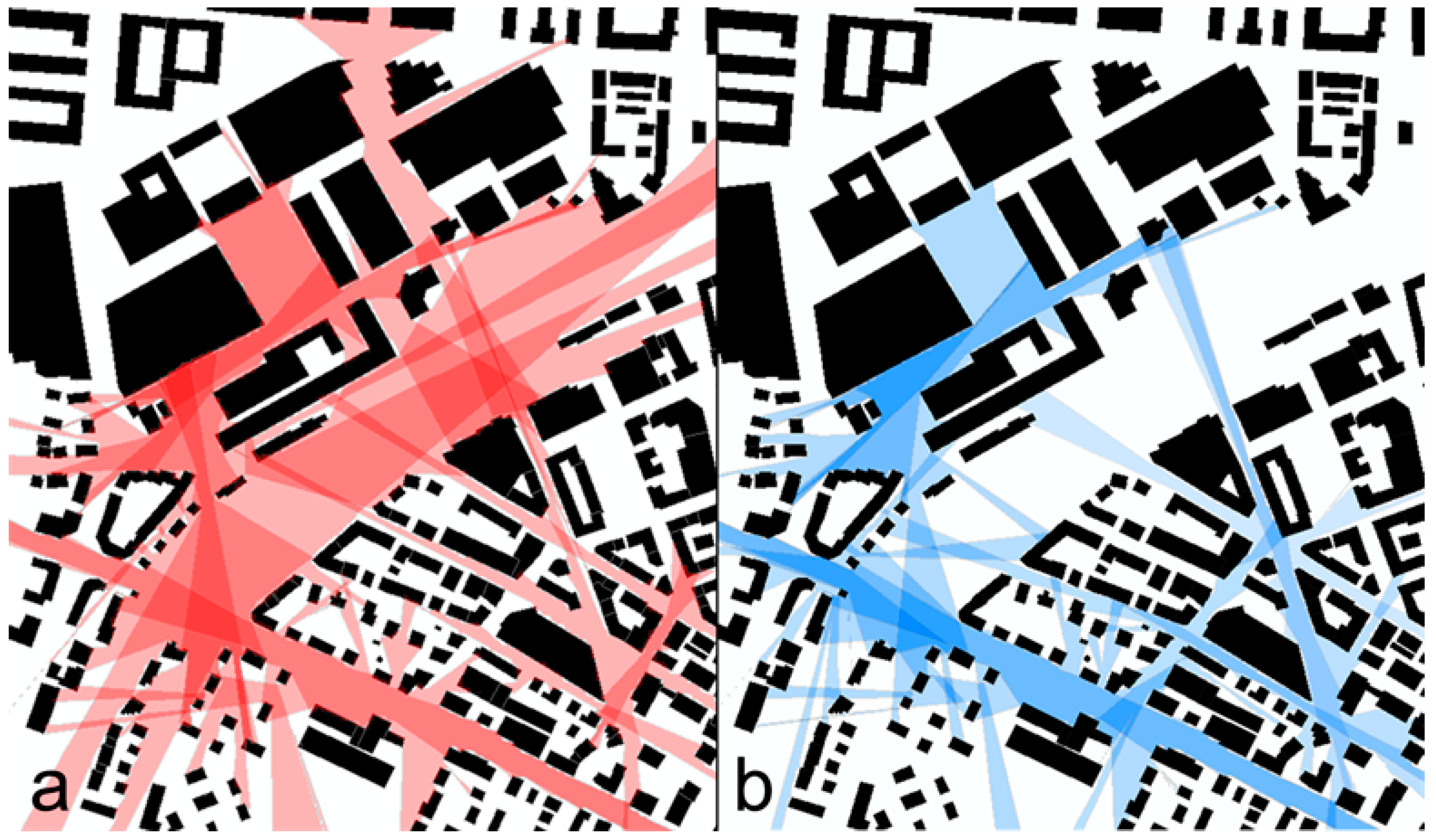
4.2. Isovist Analysis

We created an isovist analysis model in Depthmap, set the analytic accuracy to 10 m and selected 6 important isovist parameters to analyze their influence on the subjects’ emotions: isovist area, isovist perimeter, isovist compactness, occlusivity, max-visibility length and min-visibility length. Of these, the formulas for isovist compactness and occlusivity are, respectively, as follows [45]:

$$\mathrm{Compactness}=1-\frac{2\sqrt{\pi S}}{P}$$

(6)

$$\mathrm{Occlusivity}=P-P_f.$$

(7)

Here, S refers to isovist area, P refers to isovist perimeter, and P_f refers to the overall lengths of solid boundaries within the isovist area.

We performed spatial matching between the values of all isovist parameters and the 348 ESPs. The values were divided into two groups based on the valence from the independent sample t-test to analyze whether significant differences occurred between the two sets of sample average values. The results indicate that when the confidence level is 95%, all isovist parameters have dominant differences; when the confidence level is 99%, most isovist parameters—except for min-visibility length—show significant differences. Therefore, we can roughly assume that these isovist parameters may influence subjects’ emotions to a certain extent.

Regression reveals relationships that may exist between one or more independent predictors and one dependent variable. Here, we applied binary logistic regression to analyze the probability that the isovist parameters influenced subjects’ emotions. First, we used each individual isovist parameter for the regression; then, we included all the isovist parameters in the model simultaneously. Finally, the predictive effects are acquired by taking the combined parameters as variables. In this case, the response variable of the logistic regression is the valence, where 0 and 1 represent the two different states (0 represents negative emotions and 1 represents positive emotions). Assuming that the response variable equals 1 (positive), the probability is P, and the formula is as follows [46]:

$$P(y=1|X_i)=\frac{e^{{\displaystyle \sum B_i{X}_i}}}{1+e^{{\displaystyle \sum B_i{X}_i}}}$$

(8)

Here, P ∈ [0, 1], Xi refers to all six isovist parameters selected in this paper, and B_i refers to the estimated coefficient of the variable.

The prediction efficiency of the regression model can be further inspected using a receiver operating characteristic analysis (ROC), which divides the prediction probability into several critical points and obtains the corresponding sensitivity and specificity of each critical point. Taking sensitivity and specificity as the coordinate axes, the points can be connected, forming a curve. When the threshold value curve coincides with the diagonal line, it means that sensitivity and specificity each account for 50%, indicating that the analysis result has no practical meaning. However, when the judged threshold value is closer to the left corner of coordinate graph, the sample’s overlapped region is smaller and the discrimination is much stronger. Overall, the area under the curve (AUC) intuitively reflects the model’s accuracy: the larger the AUC is, the higher the accuracy is. When the Youden index is the highest, the optimal critical point can be determined as follows [47]:

$$Y=S_e-(1-S_p),$$

(9)

where Y refers to the Youden value; S_e refers to sensitivity, and S_p refers to specificity.

The results show that when using only a single isovist parameter for the logical regression, the Hosmer-Lemeshow coefficients, which reflect the model’s overall goodness-of-fit, are all less than the set significance level (p < 0.05). This indicates that the regression model does not fully extract data, and there is a dominant difference between the model’s predicted value and observed value. The results also show that the ROC curve of every individual isovist parameter is located around the coordinate’s diagonal line (Figure 6a–f), which further verifies the conclusion of the unsatisfactory regression effect. Consequently, we can judge that the emotions of subjects cannot be estimated accurately using any single isovist parameter. Therefore, after removing those isovist parameters with poor correlations, we combined the remaining isovist parameters into the regression model. Finally, we chose isovist compactness (X1), neighborhood degree (X2) and maximum visibility (X3) as the concomitant variables. To maintain the proper proportion of estimation coefficients, corresponding scaling of parameters is required. By selecting the regression method with optimal efficiency, we can carry out an iterative computation. The Hosmer-Lemeshow coefficient reaches 0.128, which is larger than the set significance level (p > 0.05). Thus, as a preliminary judgment, this model generally accepts the null hypothesis of the model fit. The regression coefficients of this comprehensive parameter model are all higher than 0.3, which conveys a certain statistical importance. The overall accuracy is 83.9%. The analysis showed that max-visibility length and isovist compactness have dominant influences on the model (

Table 2. Comprehensive parameter logical regression model.

Inspection Coefficient	Inspection Result	Prediction Coefficient	Estimated Coefficient	p-Value	Wals Value
Cox & Snell R2	0.302	X1	1.03	0.000	36.549
Nagelkerke R2	0.438	X2	0.10	0.032	4.611
Hosmer-Lemeshow	0.128	X3	0.70	0.000	14.709

). Through ROC curve analysis, the AUC value (Figure 6g) of the comprehensive parameter model is 0.849 (p < 0.05). According to experience, 0.7 < AUC < 0.9 is a prediction range with mid-level accuracy, showing that the model based on the comprehensive isovist parameter model has quite good predictive power. By taking advantage of the Youden index, we can conclude that the optimal probability division point of the comprehensive parameter model lies at approximately 0.51, which is close to the model’s default threshold value of 0.5. Therefore, we accept the predicted result judged by the model’s division point.

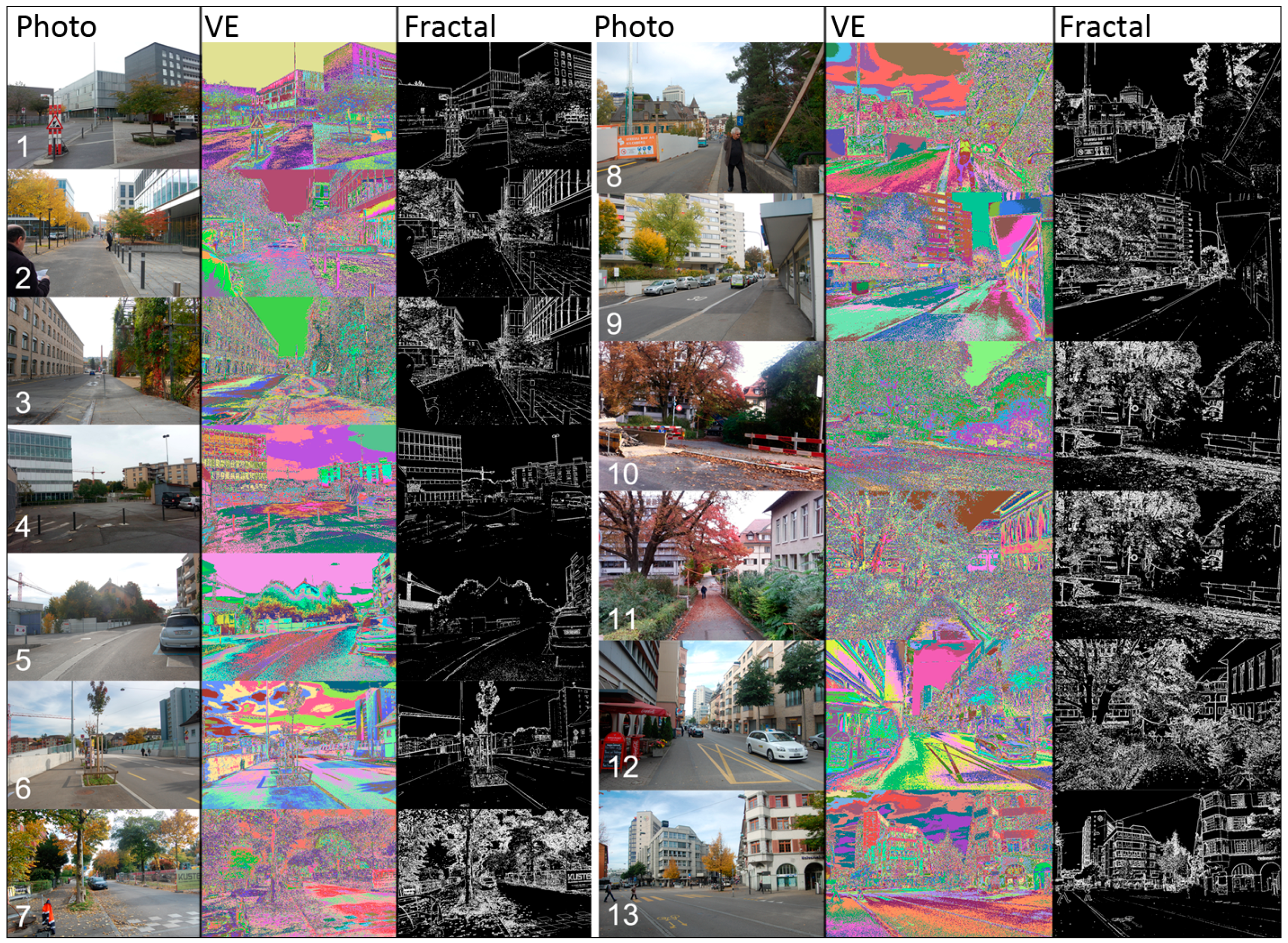
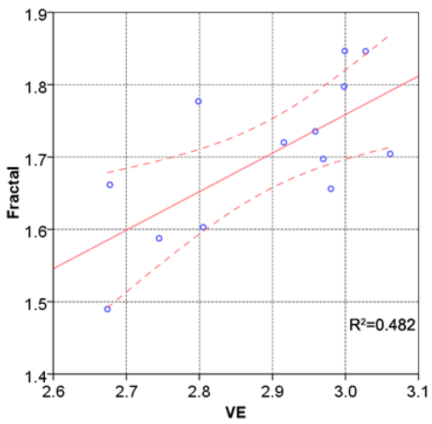
4.3. Analysis of Visual Entropy and Fractals

To gain a better understanding of how spatial attributes affect people’s emotion via their visible attributes, we further analyzed the photos taken by subjects at the locations, which show significant clustering effects as described earlier. When the human visual system perceives an image, attention is not evenly distributed. This uncertainty can be measured by the visual entropy. The concept of entropy was initially used to describe the confusion degree in thermodynamics and was introduced in information theory to represent the uncertainty of a signal source [48]. Visual Entropy (VE) is a quantitative description that reflects the visual information perceived by a subject, namely—here, the visual complexity and richness of images in an urban context. Due to the extremely high complexity of urban spaces, it is difficult to accurately measure the geometrical parameters of all the details. Thus, this paper uses real digital photos of those effective sampling points and calculates the VE values from these photos. This method has been widely applied in many psychological experiments and is highly credible [49,50,51,52]. By processing the photos into a gray-scale map with 0–255 discrete values, this paper considers each gray-scale unit as a different signal from the image signal source. The overall VE is then calculated by the distribution of pixels of each gray-scale unit using the following formula:

$$H=-{\displaystyle \sum P_i}\log P_i$$

(10)

where H denotes the image’s overall VE and P_i refers to the probability that every gray-scale pixel value appears. To eliminate noise, the threshold value was set to 3%. Signals less than the threshold value are considered not to be valid data. Only those regions where the quantity of the pixels is larger than the threshold value in the image are evaluated. To simplify the calculations, this paper divides the image’s gray-scale into 25 grades. The luminance information of the green wave band is quite sufficient as it possesses better image contrast [53]. Consequently, the gray-scale map of this band is considered in this analysis.

Furthermore, the complexity of an urban spatial environment and its visual impact on subjects can also be measured by fractals [54]. It has been argued that nature is a complicated system that has characteristics of irregularity and self-similarity [55]. Mandelbrot described these unordered and fragmentized natural forms using the concept of a “fractal.” A fractal can exist in the form of a fraction within the Euclidean dimension. For instance, an irregular shoreline is neither a one-dimensional straight line nor a two-dimensional plane. Its fractal lies between those two dimensions and up to the inflection degree of the shoreline. The key to understanding fractals lies in the selection of the measurement scale. It requires different “scales” to measure objects with fractal characteristics as well as different quantities. The fractal dimension can describe the complexity and inflection degree of an image. The larger the fractal dimension is, the more complicated the image will be. The operations in this step were also based on the analysis of the real photos. The step was conducted using the boxing-counting method as follows. First, the images were resized to 1450 × 950 pixels. The borders of all photos were intensified and transformed into gray-scale maps. Taking the gray-scale value 128 as a segmentation point, the photos were further transformed into binary graphs containing only black and white pixels. Considering the two-dimensional grids on the images; when the side length is d, the quantity of effective grids in the white part is N(d). According to the fractal principle, N(d) is the power-exponent function of d. The formula is as follows [56]:

$$N(d)=\frac{1}{d^D}.$$

(11)

For convenience of observation and calculation, a logarithmic transformation of Equation (8) was made, and the function is drawn on the double logarithmic coordinate graph. D is the fractal of this image:

$$\ln N(d)=D\ln (\frac{1}{d}).$$

(12)

By adding the VE and the fractal together, a comprehensive visual index can be obtained as follows:

$$VI=VE+D.$$

(13)

By alternately comparing the current comprehensive index with the previous index, we can observe the changing tendencies of the data, the formula for which is as follows:

$$V{I_i}^{\prime }=V{I}_i-V{I}_{i-1},$$

(14)

where $V{I_i}^{\prime }$ is the variability index of the visual index and VI_i refers to the comprehensive visual index of the sampling site. The numbers 1 and 0 are used to represent the positive and negative symbols of the calculation, matching all the sampling locations’ variability indices with the valence.

In this analysis, 13 hot-spot clusters were selected from the P and N collections for sequencing (Figure 7). Photos were matched with the shooting locations. We used a full frame camera with a 35 mm by 24 mm CCD and set the focal length to 50 mm, which results in images similar to a human field of vision. Then, based on the photos, we calculated the VE and fractal (Figure 8). Generally, photos in which all the elements are well-defined and integrated, resulting in high fractal and VE values, seem important in causing positive emotions in people; locations with positive emotions tend to present images with a strong sense of order and richness. In these areas, the buildings are arranged neatly, and the images reflect enclosed space (No. 1 and No. 2). Other than a compact and neat isovist form, the richness of plant landscapes and greening hierarchy may influence positive emotions (No. 7 and No. 11). After the test, subjects reflected that it is easier to feel a sense of safety in such spaces. According to Maslow’s theory, safety is an important precondition for pleasure, and locations with negative emotions show comparatively weak spatial order, such as weak orientation and open space (No. 4 and No. 13). Although No. 8 and No. 10 locations present high values of fractal and VE, the continuity of space is damaged due to intervening roadblocks and junk, which may be among the reasons that led subjects to experience negative emotions. Furthermore, positive and negative emotions overlap with each other in some locations, such as the No. 3 location. Those photos show quite strong cityscape contrasts. Rich landscaped vegetation and rigid architectures appear on both the left and right sides of the image simultaneously. Therefore, the emotions of subjects in such locations may change based on the objects that currently hold their attention, causing the sampled emotions in these locations to vary.

Through visual analysis of every photo location, Figure 9 shows that VE and fractal have obvious wave resonances and correlation. The Pearson coefficient of those two variables is 0.694 (the confidence level is 99%), showing a strong linear correlation. The two sets of data both have comparatively high values at the No. 7 and No. 11 locations—lush trees grow at these two locations. The visible buildings are low and mostly covered by greenery. In both images, the sky accounts for only a small proportion; the landscape dominates both photos. In contrast, the No. 5 and No. 6 locations have very low VE and fractal values. No. 6 is located at the end of a bridge across the railway and has a broad view. The landscape element has a comparatively flat visual depth because the bridge and sky account for the greater part of the view. There are few trees, and the sense of any enclosed space is weak. To properly analyze the visual differences under these two valence statuses, we divided the data for VE and fractals into two sets based on the valence and then conducted an independent t-test to compare the mean values of the two sets. The results show no significant difference overall (p > 0.05).

Additionally, valence and variability index correlate at 9 locations (

Table 3. Visual entropy and visual fractal inspection results.

Location No.	Fractal	Visual Entropy	Comprehensive Visual Index	Predicted Value	Observed Value	Inspection Result
1	1.6616	2.677428	4.339028	1	1	√
2	1.7354	2.958627	4.694027	1	1	√
3	1.7770	2.798628	4.575628	0	0	√
4	1.5876	2.744836	4.332436	0	0	√
5	1.4898	2.674102	4.163902	0	1	×
6	1.6030	2.805265	4.408265	1	0	×
7	1.8466	2.999055	4.845655	1	1	√
8	1.6561	2.979993	4.636093	0	0	√
9	1.7202	2.915624	4.635824	0	0	√
10	1.7974	2.998140	4.79554	1	0	×
11	1.8463	3.027640	4.87394	1	1	√
12	1.7044	3.061204	4.765604	0	1	×
13	1.6973	2.969658	4.666958	0	0	√

), accounting for 70% of the 13 total locations. To a certain extent, this supports the prior assumptions, namely, that changes in emotion cannot be judged merely by isovist parameters. In addition to the comprehensive impact of all kinds of visual factors, emotion changes in the subjects were also related to the sequence in which people experienced the spaces. In addition, the switching node (e.g., crossroads and street corners) usually has significant effects. Such an influence is, moreover, affected by time. When subjects enter the next switching space, they will consciously compare it with the former node and its spatial attributes. The comprehensive differences between these two sets of spatial attributes may constitute an important trigger for changes in emotion.

5. Discussion and Conclusion

This paper investigated the correlative coupling effects between urban spatial attributes and people’s subjective emotions using a combination of quantitative analysis and qualitative description. The results show that the attributes of urban spaces and visual factors do possess complicated characteristics that affect people’s emotions. While making this summary, this paper proposes some further discussion points as follows:

• People’s emotions are affected by different building layouts—in particular, how people perceive the spaces between buildings. Among those factors, isovist scope and relevant attributes are important ways for people to obtain visual information during their urban experience. Pedestrians activities in urban spaces are not simply restricted to any single isovist parameter but to the comprehensive impact of several isovist parameters, of which compactness, occlusivity, and maximum visibility are comparatively dominant. Among the three, higher compactness and greater visibility within a space seem to be advantageous in causing positive emotions, indicating that people may prefer spaces with good vistas within a suitable distance and clearer boundaries. However, this does not mean that people prefer an unlimited field of view. Large unending avenues might be monotonous and boring. A threshold effect may occur, and that is the question our future research will seek to answer.
• Spatial attributes are not merely reflected in planar isovist form; the richness and complexity of three-dimensional space are also important reasons affecting the spatial experience of pedestrians. Visual information analysis can help designers effectively interpret the qualities of an urban space. According to this research, enclosed urban spaces are very important in fostering a sense of security in pedestrians. During the process of urban planning and design, specific entity borders, neat and compact isovist forms, a rich landscape hierarchy and greenery are easy ways to create urban spaces with a sense of place. Some man-made obstacles can seriously weaken the qualities of the spatial environment. Only by strengthening management and daily maintenance is it possible to ensure the design achievements, which are hard to obtain, and maintain a spatial environment with positive qualities.
• Human perception of urban space tends to focus on important spatial nodes; therefore, we cannot neglect changes in the spatial sequence or the design treatment of spatial nodes. These should strengthen the systematic construction of urban spatial nodes, including public squares, street greening, and street corners. The integration of points, lines and networks—especially those that reinforce the continuity and network of pedestrian space—should give full weight to the way in which the scenes of these spatial nodes switch and cultivate urban spatial sequences with special meanings that reinforce positive images during urban movement.

Finally, the findings of the presented study motivated us to undertake a more comprehensive study aimed at obtaining more significant results. The sample sizes in this study and in all the related studies mentioned earlier were small. Our more comprehensive study is being performed in the ongoing research project ESUM (http://www.ia.arch.ethz.ch/esum/), for which we developed a sensor backpack that gathers considerably more data from the urban environment. This will be a novel data collection process for Smart Cities that includes (i) environmental data, such as noise, dust, illuminance, temperature, relative humidity; (ii) location/mobility data, such as GPS and occupant density detected via WiFi; and (iii) perceptual social data, collected by citizens’ responses using smart phones. These fine-grained real-time data can provide additional insights about the spatial correlations between urban environments and emotional responses of the inhabitants.

However, people’s emotions may be affected by many other complicated factors such as building façade details, building functions, and what individuals actually see. To clarify the manifold influences concerning the relationships between people’s emotions and built environments, we need to develop a more solid and accurate theoretical framework for future research.

References

- Alexander, E.R.; Reed, K.D.; Murphy, P. Density Measures and Their Relation to Urban Form: Center for Architecture and Urban Planning Research; University of Wisconsin: Milwaukee, MI, USA, 1988. [Google Scholar]
- Herrera-Yagüe, C.; Schneider, C.M.; Couronne, T.; Smoreda, Z.; Benito, R.M.; Zufiria, P.J.; González, M.C. The anatomy of urban social networks and its implications in the searchability problem. Sci. Rep. 2015. [Google Scholar] [CrossRef] [PubMed]
- Lang, J. Urban Design: The American Experience; John Wiley & Sons: New York, NY, USA, 1994. [Google Scholar]
- Trancik, R. Finding Lost Space: Theories of Urban Design; John Wiley & Sons: New York, NY, USA, 1986. [Google Scholar]
- Noulas, A.; Scellato, S.; Lambiotte, R.; Pontil, M.; Mascolo, C. A tale of many cities: Universal patterns in human urban mobility. PLoS ONE 2012, 7, e37027. [Google Scholar] [CrossRef]
- Polsky, C.; Grove, J.M.; Knudson, C.; Groffman, P.M.; Bettez, N.; Cavender-Bares, J.; Larson, K.L. Assessing the homogenization of urban land management with an application to US residential lawn care. Proc. Natl. Acad. Sci. USA 2014, 111, 4432–4437. [Google Scholar] [CrossRef] [PubMed]
- Expert, P.; Evans, T.S.; Blondel, V.D.; Lambiotte, R. Uncovering space-independent communities in spatial networks. Proc. Natl. Acad. Sci. USA 2011, 108, 7663–7668. [Google Scholar] [CrossRef] [PubMed]
- Franck, K.; Stevens, Q. Loose Space: Possibility and Diversity in Urban Life; Routledge: New York, NY, USA, 2013. [Google Scholar]
- Gehl, J. Life between Buildings: Using Public Space; Island Press: Washington, DC, USA, 2011. [Google Scholar]
- Gospodini, A. Urban design, urban space morphology, urban tourism: An emerging new paradigm concerning their relationship. Eur. Plan. Stud. 2001, 9, 925–934. [Google Scholar] [CrossRef]
- Sun, L.; Axhausen, K.W.; Lee, D.H.; Huang, X. Understanding metropolitan patterns of daily encounters. Proc. Natl. Acad. Sci. USA 2013, 110, 13774–13779. [Google Scholar] [CrossRef] [PubMed]
- Hillier, B.; Iida, S. Network and psychological effects in urban movement. In Spatial Information Theory; Lecture Notes in Computer Science; Springer: Berlin/Heidelberg, Germany, 2005; pp. 475–490. [Google Scholar]
- Hillier, B. Space is the Machine: A Configurational Theory of Architecture; Cambridge University Press: Cambridge, MA, USA, 1996. [Google Scholar]
- Clifford, C.W.G.; Rhodes, G. Fitting the Mind to the World: Adaptation and After-Effects in High-Level Vision; Oxford University Press: Oxford, UK, 2005. [Google Scholar]
- Stamps, A.E. Advances in visual diversity and entropy. Environ. Plan. B Plan. Des. 2003, 30, 449–463. [Google Scholar] [CrossRef]
- Dalton, R.C. The secret is to follow your nose route path selection and angularity. Environ. Behav. 2003, 35, 107–131. [Google Scholar] [CrossRef]
- Wiener, J.M.; Hölscher, C.; Büchner, S.; Konieczny, L. Gaze behaviour during space perception and spatial decision making. Psychol. Res. 2012, 76, 713–729. [Google Scholar] [CrossRef] [PubMed]
- Franz, G.; Wiener, J.M. From space syntax to space semantics: A behaviorally and perceptually oriented methodology for the efficient description of the geometry and topology of environments. Environ. Plan. B Plan. Des. 2008, 35, 574–592. [Google Scholar] [CrossRef]
- Ewing, R.; Handy, S. Measuring the unmeasurable: Urban design qualities related to walkability. J. Urban Des. 2009, 14, 65–84. [Google Scholar] [CrossRef]
- Handy, S.L.; Boarnet, M.G.; Ewing, R.; Killingsworth, R.E. How the built environment affects physical activity: Views from urban planning. Am. J. Prev. Med. 2002, 23, 64–73. [Google Scholar] [CrossRef]
- Morello, E.; Ratti, C. A digital image of the city: 3D isovists in Lynch’s urban analysis. Environ. Plan. B Plan. Des. 2009, 36, 837–853. [Google Scholar] [CrossRef]
- Batty, M. Agents, cells, and cities: New representational models for simulating multiscale urban dynamics. Environ. Plan. A 2005, 37, 1373–1394. [Google Scholar] [CrossRef]
- Seto, K.C.; Reenberg, A.; Boone, C.G.; Fragkias, M.; Haase, D.; Langanke, T.; Simon, D. Urban land teleconnections and sustainability. Proc. Natl. Acad. Sci. USA 2012, 109, 7687–7692. [Google Scholar] [CrossRef] [PubMed]
- Wu, J.; Jelinski, D.E.; Luck, M.; Tueller, P.T. Multiscale analysis of landscape heterogeneity: Scale variance and pattern metrics. Geogr. Inf. Sci. 2000, 6, 6–19. [Google Scholar] [CrossRef] [PubMed]
- Rattenbury, T.; Naaman, M. Methods for extracting place semantics from Flickr tags. ACM Trans. Web 2009, 3, 1139–1141. [Google Scholar] [CrossRef]
- Wakamiya, S.; Belouaer, L.; Brosset, D.; Lee, R.; Kawai, Y.; Sumiya, K.; Claramunt, C. Measuring crowd mood in city space through twitter. In Web and Wireless Geographical Information Systems; Springer International Publishing: Cham, Switzerland, 2015; pp. 37–49. [Google Scholar]
- Resch, B.; Summa, A.; Zeile, P.; Strube, M. Citizen-centric urban planning through extracting emotion information from twitter in an interdisciplinary space-time-linguistics algorithm. Urban Plan. 2016, 1, 114–127. [Google Scholar] [CrossRef]
- Resch, B.; Sudmanns, M.; Sagl, G.; Summa, A.; Zeile, P.; Exner, J.P. Crowdsourcing physiological conditions and subjective emotions by coupling technical and human mobile sensors. GIForum J. Geogr. Inf. Sci. 2015, 1, 514–524. [Google Scholar] [CrossRef]
- Academy of Neuroscience for Architecture. 2013. Available online: http://www.anfarch.org/ (accessed on 20 October 2016).
- Peters, D.; Richter, K. Taking off to the third dimension: Schematization of virtual environments. Int. J. Spat. Data Inf. Res. 2008, 3, 20–37. [Google Scholar]
- Russell, J.A. A circumplex model of affect. J. Personal. Soc. Psychol. 1980, 39, 1161–1178. [Google Scholar] [CrossRef]
- Emotions of the Urban Pedestrian: Sensory Mapping. Available online: http://www.walkeurope.org/uploads/File/publications/PQN%20Final%20Report%20part%20B4.pdf#page=32 (accessed on 20 October 2016).
- Bergner, B.S.; Exner, J.P.; Memmel, M.; Raslan, R.; Dina-Taha, D.; Talal, M.; Zeile, P. Human sensory assessment methods in urban planning: A case study in Alexandria. Proc. REAL CORP 2013, 1, 407–417. [Google Scholar]
- Mavros, P.; Coyne, R.; Roe, J.; Aspinall, P. Engaging the brain: Implications of mobile EEG for spatial representation. In Proceedings of the 30th International Conference on Education and Research in Computer Aided Architectural Design in Europe, Prague, Czech Republic, 12–14 September 2012.
- Camras, L.A.; Meng, Z.L.; Ujiie, T.; Dharamsi, S.; Miyake, K.; Oster, H.; Campos, J. Observing emotion in infants: Facial expression, body behavior, and rater judgments of responses to an expectancy-violating event. Emotion 2002, 2, 179–193. [Google Scholar] [CrossRef] [PubMed]
- Solomon, R.C. Back to basics: On the very idea of “basic emotions”. J. Theory Soc. Behav. 2002, 32, 115–144. [Google Scholar] [CrossRef]
- Fabrikant, S.I.; Christophe, S.; Papastefanou, G.; Maggi, S.; Fabrikant, S.I.; Maggi, S. Emotional response to map design aesthetics. In Proceedings of the GIScience Conference 2012, Columbus, OH, USA, 18–21 September 2012.
- Bodymonitor. Available online: http://www.bodymonitor.de/ (accessed on 20 October 2016).
- Papastefanou, J. Experimentelle Validierung eines Sensorarmbandes zur mobilen Messung physiologischer Stressreaktionen. GESIS-Tech. Rep. 2013, 7, 1–14. [Google Scholar]
- Zhang, S.L.; Zhang, K. Comparison between General Moran’s index and Getis-Ord General G of spatial autocorrelation. Acta Sci. Nat. Univ. Sunyatseni 2007, 46, 93–97. [Google Scholar]
- Getis, A.; Ord, J.K. The analysis of spatial association by use of distance statistics. Geogr. Anal. 1992, 24, 189–206. [Google Scholar] [CrossRef]
- Ord, J.K.; Getis, A. Local spatial autocorrelation statistics—Distributional issues and an application. Geogr. Anal. 1995, 27, 286–306. [Google Scholar] [CrossRef]
- Benedikt, M.L. To take hold of space—Isovists and isovist fields. Environ. Plan. B Plan. Des. 1979, 6, 47–65. [Google Scholar] [CrossRef]
- Davis, L.S.; Benedikt, M.L. Computational models of space: Isovists and isovist fields. Comput. Graph. Image Proc. 2003, 11, 49–72. [Google Scholar] [CrossRef]
- Forman, R.T.T.; Godron, M. Landscape Ecology; John Wiley & Sons: New York, NY, USA, 1986. [Google Scholar]
- Harrell, F.E.X. Regression Modeling Strategies: With Applications to Linear Models, Logistic Regression, and Survival Analysis; Springer Science Business Media: Berlin, Germany, 2013. [Google Scholar]
- Fawcett, T. An introduction to ROC analysis. Pattern Recogn. Lett. 2006, 27, 861–874. [Google Scholar] [CrossRef]
- Segal, I.E. A note on the concept of entropy. J. Math. Mech. 1960, 9, 623–629. [Google Scholar] [CrossRef]
- Berlyne, D.E.; Madsen, K.B. Pleasure, Reward, Preference: Their Nature, Determinants, and Role in Behavior; Academic Press: New York, NY, USA, 2013. [Google Scholar]
- Cooper, J.; Oskrochi, R. Fractal analysis of street vistas: A potential tool for assessing levels of visual variety in everyday street scenes. Environ. Plan. B Plan. Des. 2008, 35, 349–363. [Google Scholar] [CrossRef]
- Stamps, A.E. Entropy, visual diversity, and preference. J. Gen. Psychol. 2002, 129, 300–320. [Google Scholar] [CrossRef] [PubMed]
- Stamps, A.E. On shape and spaciousness. Environ. Behav. 2008, 41, 526–548. [Google Scholar] [CrossRef]
- Sato, T.; Matsuoka, M.; Takayasu, H. Fractal image analysis of natural scenes and medical images. Fractals Int. J. Complex Geom. Nat. 1996, 4, 463–468. [Google Scholar] [CrossRef]
- Jiang, B.; Sui, D.Z. A new kind of beauty out of the underlying scaling of geographic space. Prof. Geogr. 2014, 66, 676–686. [Google Scholar] [CrossRef]
- Mandelbrot, B.B. Fractals—Form, Chance, and Dimension; W.H.Freeman & Company: New York, NY, USA, 1977. [Google Scholar]
- Li, J.; Du, Q.; Sun, C.X. An improved box-counting method for image fractal dimension estimation. Pattern Recognit. 2009, 42, 2460–2469. [Google Scholar] [CrossRef]