Aggregated Epidemic Localization and Spatiotemporal Diffusion Modeling Considering Road Network-Constrained Spatial Clustering and Tensor Field Analysis: A Case Study of COVID-19

Abstract

Aggregated epidemics, characterized by rapid transmission over short periods, pose severe threats to public health security, necessitating the development of precise source tracing and simulation methods to support efficient prevention and control. However, existing studies suffer from three major gaps: (1) predominant focus on national/regional scales with limited urban-scale analysis; (2) reliance on proprietary mobile data that are often inaccessible; and (3) NP-hard computational complexity in traditional source tracing methods. To bridge these gaps, this paper proposes an integrated spatiotemporal diffusion model comprising two core components: outbreak point estimation and spatial diffusion simulation. The model first uses the SEAIR infectious disease dynamics model to predict trends, combines the 3-Sigma criterion and viral incubation period to screen early epidemiological survey data, employs a road network-constrained DBSCAN algorithm for spatial clustering, and locates the outbreak point via an improved inverse distance weighting method incorporating time and POI density weights. Subsequently, using the estimated outbreak point as the initial transmission center, and based on the “cell-type” living structure hypothesis of populations, it fuses multi-source geographic data to quantify regional attractiveness and simulate viral diffusion in grid space. The model is validated using COVID-19 epidemic data from Xi’an, Shanghai, and the Hong Kong Special Administrative Region of China. Results show that the proposed outbreak point estimation method effectively estimates the initial transmission center, with distances between estimated points and officially announced points of 0.786 km, 1.676 km, and 5.441 km, respectively—shortened by 179 m, 1091 m, and 711 m compared to related studies. The spatiotemporal diffusion model effectively simulates daily incidence patterns, achieving average coverage rates of 67.32% and 72.9% and average precision rates of 60.67% and 78.84% in Shanghai and Hong Kong, respectively, with significantly better simulation accuracy than traditional methods in the early and middle stages of the epidemic. This study provides a scientifically robust, data-parsimonious framework for precise source tracing, early warning, and resource allocation in urban epidemics, with strong generalizability to other resource-limited settings.

1. Introduction

Emerging and re-emerging infectious diseases remain major challenges to global public health security [1]. Among them, aggregated epidemics—defined as a significant excess of cases in specific settings or populations over a short period [2]—are a special and highly harmful form of transmission. Characterized by strong suddenness, rapid spread, and concentrated scope, they easily trigger chain reactions in medical institutions, schools, factories, and communities, leading to exponential growth in cases and immense pressure on prevention and control [3]. During the COVID-19 pandemic, aggregated epidemics frequently occurred and became key nodes driving epidemic development [4]. Despite the approval and large-scale deployment of vaccines (e.g., COVID-19 vaccines) and oral antivirals (e.g., Paxlovid, Ritonavir, Simnotrelvir Tablets), limitations in timeliness and accessibility of drug interventions persist in resource-poor regions or during early stages of new variant emergence. Against this backdrop, developing technologies and methods for rapid identification, precise source tracing, and effective simulation of aggregated epidemic spatiotemporal diffusion remains crucial for implementing efficient non-pharmaceutical interventions (e.g., lockdowns, epidemiological surveys, testing) to reduce transmission speed and socio-economic losses [5].

Computer modeling and simulation have become indispensable tools for understanding and predicting infectious disease transmission dynamics [6]. Classic compartmental models (e.g., SIR, SEIR) describe population infection state evolution macroscopically [7]; cellular automata models discretize space to simulate local rule-based diffusion [8]; complex network-based models reveal transmission heterogeneity and key nodes by constructing contact networks between individuals or regions [9]; and agent-based models achieve high-fidelity simulation by assigning behavioral rules to individuals [10]. In recent years, with enhanced availability of multi-source geospatial data (e.g., mobile location, traffic flow, points of interest (POIs)), research combining spatiotemporal analysis and visualization for infectious disease transmission has gained momentum [11,12,13]. For example, knowledge graphs have been used to construct case activity trajectories for epidemic situation analysis [14,15]; visual analysis methods have been applied to anomaly detection and air pollution exploration [16,17]. These studies provide rich methodological references for infectious disease spatiotemporal analysis. What’s more, A growing body of international research has highlighted that COVID-19 transmission is deeply shaped by combined spatial, social, economic, and environmental factors, underscoring the value of integrated spatial–social approaches in global epidemic studies. In the context of sub-Saharan Africa, Abdollahi and Behzadi used spatial regression and cluster detection techniques to show that population density, urbanization level, and healthcare access significantly influenced the geographic distribution of COVID-19 cases and mortality risks [18]. Focusing on Bangladesh, Sarkar et al. applied spatial lag and error models to reveal strong associations between population mobility, urban density, and the spatial clustering of infections, emphasizing the role of social activity patterns in shaping outbreak hotspots [19]. Furthermore, in a comprehensive spatial analysis of Brazil, Silva et al. explored how socioeconomic inequalities, urban form, and environmental conditions jointly drove heterogeneous transmission dynamics across different regional contexts, demonstrating that epidemic patterns cannot be fully understood without considering local social and geographic realities [20]. Collectively, these global studies confirm that COVID-19 spread is a socially embedded spatial process, requiring models that account for real-world urban structures, human mobility, and socio-demographic conditions.

However, in the context of precise prevention and control of clustered epidemics, existing research still faces three prominent challenges that correspond to the gaps identified in recent critical reviews. First, a spatial scale gap persists. As summarized in the [21], over 90.9% of existing COVID-19 studies focus on national or large regional scales, leaving a significant gap in urban-scale (4.7%) analysis. Most models rely on coarse administrative boundaries, which fail to capture intra-urban heterogeneity in transmission dynamics. Second, there is a data scarcity challenge. In epidemiological studies involving GIS-based spatial analysis, the existing research predominantly relies on mobility data sources such as mobile signaling data, transportation system records, and various types of sensor data. However, in practical research scenarios, obtaining such rich and complete mobility observations often faces high barriers. At the same time, due to limitations in data collection capabilities across different regions or time periods, mobility data often suffer from incomplete coverage or missing values (as discussed in the context of “a paradigm shift in observation under data scarcity” in Literature [22]). Third, methodological limitations in source localization lead to NP-hard computational complexity. Source localization methods abstract contact tracing data into network nodes, estimate transmission parameters via SEIR or multi-source data (e.g., mobile phone data), and construct a global objective function. However, as the node scale expands, the problem becomes NP-hard. Consequently, existing studies rely on heuristic optimization algorithms, which can only guarantee locally optimal solutions rather than global optimality [23].

To address these challenges, literature [24] proposes a discrete-grid spatio-temporal diffusion model based on population life characteristics, centered on estimating the outbreak source and using a tree-like travel structure to quantify inter-grid flow weights. However, its characterization of spatial heterogeneity and road network constraints remains limited. This paper constructs an integrated spatiotemporal diffusion model framework using COVID-19 aggregated epidemics as empirical research objects. Compared with [24], the proposed framework introduces three key methodological advancements. First, road-network-constrained accessibility analysis replaces the Euclidean-distance-based circular buffer, better aligning with actual human movement behaviors. Second, a cell-based local interaction structure is adopted instead of a tree-like travel hierarchy; Third, CP tensor decomposition is employed to dynamically derive spatially varying infection probabilities, overcoming the limitation of the uniform empirical probability used in [24]. This enhancement enables the model to account for urban heterogeneity, thereby improving its robustness and applicability across diverse cities.

The main contributions of this paper are as follows:

(1)

Proposing a two-stage modeling framework that organically links outbreak point estimation and spatiotemporal diffusion simulation, providing a systematic methodology for full-process analysis of aggregated epidemics from “source tracing” to “prediction”.

(2)

In outbreak point estimation, creatively integrating infectious disease dynamics, statistical process control, and spatial data analysis. Through four steps—SEAIR model-based trend prediction, 3-Sigma criterion-based stage identification, road-network-constrained DBSCAN clustering guided by potential field theory, and spatiotemporal-environmental weight-based localization—it significantly enhances the ability to locate epidemic sources in early stages with sparse and noisy data, while avoiding NP-hard complexity. Experiments in Xi’an, Shanghai, and Hong Kong show superior estimation accuracy compared to existing methods.

(3)

In diffusion simulation, proposing the “cell-type” living structure hypothesis and designing a method combining tensor decomposition-based POI attraction quantification and multi-source geographic data fusion to generate a driving attraction field. This model replaces inaccessible mobile data with widely available POI data, and supports multi-granularity (10 m, 100 m, 200 m, 250 m, 500 m, 1 km, 2 km, etc.) simulation, achieving finer, more realistic spatial simulation than traditional macro models under feasible data conditions, with good coverage and precision rates in early and middle stages of epidemics in Shanghai and Hong Kong.

2. Materials and Methods

2.1. Study Areas

To comprehensively verify the method’s universality, robustness, and adaptability to different urban environments, three representative first-tier cities/special administrative regions in China were selected: Xi’an, Shanghai, and Hong Kong. These regions experienced large-scale, distinct COVID-19 aggregated epidemics from late 2021 to 2022, with relatively complete publicly available epidemic data, epidemiological survey information, and basic geographic data, meeting the needs for multi-source data validation.

• Xi’an: As the core city of Northwest China, it reported its first local confirmed case on 9 December 2021. The epidemic spread rapidly, forming complex aggregated epidemics with intertwined transmission chains, and was basically controlled by 18 January 2022, with 2050 cumulative confirmed cases. This case has detailed data and complete published trajectory information;
• Shanghai: As an international metropolis and national economic center, it experienced a severe Omicron variant epidemic rebound starting 1 March 2022, lasting over two months with peak daily new cases exceeding 20,000. This case has high population density and mobility, but published epidemiological data is coarse-grained (mainly residential addresses), challenging the model’s ability to handle incomplete information;
• Hong Kong: As a highly prosperous international city, it was hit by the fifth wave of the epidemic from January to March 2022, mainly caused by the Omicron variant with extremely rapid transmission. This case features unique high-density residential environments (e.g., “public housing estates”) and an international background, with data sources differing from mainland cities.

2.2. Data Sources

Five types of data were collected and processed, with all spatial data unified to the WGS84 geographic coordinate system.

2.2.1. Epidemic Infection Data

The epidemic data for Xi’an City and Shanghai City were both sourced from their respective Municipal Health Commissions, while the epidemic data for Hong Kong came from the Centre for Health Protection (CHP) under its Department of Health.

Table 1. Summary of Urban Epidemic Data Sources.

City	Epidemic Outbreak Time	Data Source
Xi’an	9 December 2021~20 January 2022	http://xawjw.xa.gov.cn/ztzl/fyfk/gzdt/ (accessed on 28 January 2022)
Shanghai	1 March 2022~11 May 2022	https://wsjkw.sh.gov.cn/yqtb/ (accessed on 13 May 2022)
Hong Kong	14 January 2022~21 March 2022	https://www.chp.gov.hk/sc/ (accessed on 30 March 2022)

summarizes the time periods and sources of data for each city, primarily used for SEAIR model fitting and prediction. The original data page of Xi’an City (https://data.gov.hk/sc-data/dataset/ accessed on 16 September 2026) is no longer available at that address. Therefore, daily counts of laboratory-confirmed COVID-19 cases in Xi’an were compiled from official press conference bulletins. These bulletins, which report on the epidemic situation in Xi’an, were retrieved from the Shaanxi Provin-cial People’s Government website. For instance, the bulletin released on 7 January 2022, which provides cumulative data up to 5 January 2022, is available at: https://www.shaanxi.gov.cn/xw/sxyw/202201/t20220107_2206781_wap.html, accessed on 16 September 2026.

2.2.2. Patient Epidemiological Survey Data

Patient epidemiological survey data includes activity trajectory points or residential address information of confirmed cases within a certain period prior to symptom onset or positive testing. As shown in

Table 2. Summary of Urban Patient Epidemiological Survey Data Sources.

City	Epidemic Outbreak Time	Data Source
Xi’an	9 December 2021~20 January 2022	https://weibo.com/huashangbao (accessed on 28 January 2022)
Shanghai	1 March 2022~11 May 2022	https://wsjkw.sh.gov.cn/yqtb/ (accessed on 13 May 2022)
Hong Kong	14 January 2022~21 March 2022	https://data.gov.hk/sc-data/dataset/hk-dh-chpsebcddr-novel-infectious-agent (accessed on 30 March 2022)

, trajectory data for Xi’an were collated from official survey reports by media (e.g., Huashang Daily); Shanghai data came from residential address information published by the Municipal Health Commission; Hong Kong data were obtained from case data by residential area on the “Data One Stop” platform (data.gov.hk, accessed on 16 September 2026). All textual addresses were geocoded to GCJ-02 coordinates using the Amap Web Service API v3 (AutoNavi Soft-ware Co., Ltd., Beijing, China). The resulting coordinates were approximately converted to the WGS-84 datum using the open-source Python package coordTransform_py (commit 7f3a91c, https://github.com/wandergis/coordTransform_py, accessed 10 July 2020) to enable overlay on WGS-84 basemaps. Typical residuals are on the order of several metres. The matching approach follows a structured address-parsing protocol, returning the highest-confidence candidate for each record. A quality-control process was implemented, including manual spot-checks of ambiguous addresses and spatial cross-validation (e.g., verifying that coordinates fall within the study area boundaries).

We acknowledge that the ambiguity of textual data inevitably introduces some errors in the outbreak source estimation. Although the geocoding process underwent rigorous quality control, inherent positional uncertainty remains a common challenge in spatial epidemiological analysis [25,26]. Studies on online geocoding services indicate that positional errors typically range from tens to hundreds of meters [27]. Such positional uncertainty may affect the subsequent spatial clustering and outbreak source localization, potentially causing deviations in cluster centers or initial points for diffusion simulations. However, this framework is designed as an auxiliary decision support tool aimed at rapidly narrowing down the potential outbreak range, rather than providing deterministic precision localization. In practical epidemic investigation and control, decision-makers typically do not focus on a single precise coordinate. Instead, they use the estimated outbreak point (or area) as the center and implement graded responses by expanding 5 km, 10 km, 20 km, etc., to establish different investigation and prevention strategies, allocating different levels of manpower and resources. Therefore, this level of error is acceptable, and the spatial errors generated by this framework can be largely compensated for in practical applications through such a “point-to-area” prevention and control strategy. We relate this issue to the limitations of the present study, and future work could integrate multi-source geocoding or higher-precision positioning data to further reduce positional uncertainty.

2.2.3. Urban Traffic Road Network Data

Vector data of main roads (highways, urban trunk roads, secondary roads, etc.) for each city were downloaded from OpenStreetMap (OSM, https://download.geofabrik.de, accessed on 16 September 2026). This data was used to construct a road network graph model as the basis for distance calculation in spatial clustering, replacing unrealistic Euclidean distances.

2.2.4. Points of Interest (POI) Data

POI Data was obtained via programming interfaces from Amaps (AutoNavi Soft-ware Co., Ltd., Beijing, China), November 2021 version. POI Data covered seven categories: catering/shopping, life services, residential communities,, corporate enterprises, science/education/culture, medical care, and scenic spots. Original coordinates (GCJ-02) were unified to WGS84. POI data characterize urban functional density and human aggregation potential.

2.2.5. Auxiliary Geographic Data

The auxiliary geographic data employed in this study consist of four categories: nighttime light data, population distribution data, land use data, and basic administrative divisions. All datasets were selected and validated to ensure temporal consistency with the 2021–2022 epidemic period under investigation, to minimize potential biases in the estimation of attraction fields and diffusion simulation results.

Among them, the Luojia-1A satellite nighttime light data, acquired on 13 June 2018, with a spatial resolution of 130 m, are adopted to indirectly reflect the intensity of regional economic and human activities. The 100 m resolution WorldPop raster (2020 version) characterizes population density heterogeneity. Rigorously validated against official census data with high spatial accuracy, it is employed in this study. In addition, the FROM-GLC land use dataset (2018 version) is applied to identify urban built-up areas, green spaces, water bodies and other land cover types, which supports the determination of traversable regions. Finally, basic administrative division data aligned with the latest official administrative boundary standards are used for data clipping and spatial boundary definition.

2.3. Methods

This study proposes a two-stage integrated modeling framework aimed at addressing two core issues of clustered epidemics: from “outbreak source tracing” to “spatiotemporal simulation”.

Stage 1 (Outbreak source tracing): based on early epidemic time-series data and patient spatial data, the outbreak point estimation module outputs the most probable initial transmission source location, solving the problem of “outbreak source tracing”.

Stage 2 (Spatiotemporal diffusion simulation): The estimated outbreak source location, together with multi-source geographic data, is fed into the spatiotemporal diffusion simulation module to model the spatial spread of the epidemic over time, addressing the issue of “balancing data granularity and simulation accuracy”.

The two stages form a closed analytical loop: Stage 1 provides the spatial origin for Stage 2, which simulates the spatial mechanism of spread as an auxiliary decision-support tool.

2.3.1. Outbreak Point Estimation Model Considering Population Mobility and Viral Incubation Period

This model aims to reverse-estimate the initial outbreak location from early, potentially noisy and delayed epidemiological survey data. It includes three sequential submodules.

Module 1: Epidemic Stage Division and Data Screening Based on SEAIR Model and 3-Sigma Criterion

To identify the inflection point where the epidemic transitions from “latent period” to “rapid rise period” and eliminate interference from large-scale population mobility in later stages, an extended SEAIR compartmental model [28] is first used to fit and predict epidemic development. Based on the SEIR model, it distinguishes asymptomatic (A) and symptomatic (I) infected individuals and considers quarantine status (ID), aligning with COVID-19 prevention realities. The model’s kinetic equations are as follows:

$$\lambda ={\displaystyle \frac{\beta (\alpha A+I)}{(N-ID)}}$$

(1)

$${\displaystyle \frac{dS}{dt}}=-\lambda S$$

(2)

$${\displaystyle \frac{dE}{dt}}=\lambda S-\sigma E$$

(3)

$${\displaystyle \frac{dA}{dt}}=\nu \sigma E-(\theta +{\gamma }_A)A$$

(4)

$${\displaystyle \frac{dI}{dt}}=(1-\nu )\sigma E-(\phi +{\gamma }_I+d_I)I$$

(5)

$${\displaystyle \frac{d\left(ID\right)}{dt}}=\theta A+\phi I-({\gamma }_{ID}+d_{ID})\left(ID\right)$$

(6)

$${\displaystyle \frac{dR}{dt}}={\gamma }_{ID}\left(ID\right)+{\gamma }_{A}A+{\gamma }_{I}I$$

(7)

where S, E, A, I, ID and R represent the number of susceptible, exposed, asymptomatic infected, symptomatic infected, quarantined, and recovered individuals, respectively; N denotes the total population of the study area; β is the effective transmission rate; α is the relative transmissibility reduction factor of asymptomatic infections compared with symptomatic infections; σ is the transition rate from the exposed state (E) to the infectious state, representing the reciprocal of the average incubation period.; ν is the proportion of exposed transitioning to asymptomatic; γ is the recovery rate; dis the disease fatality rate; θ and φ are the detection rates of asymptomatic and symptomatic infected, respectively. ${\gamma }_A$ is the recovery rate of asymptomatic infected individuals (A); ${\gamma }_I$ is the recovery rate of symptomatic infected individuals (I); ${\gamma }_{ID}$ is the recovery rate of quarantined individuals (ID); $dI$ is the disease-induced mortality rate of symptomatic infected individuals (I); $d\left(ID\right)$ is the disease-induced mortality rate of quarantined individuals (ID).

Using the early epidemic data (e.g., the first 10, 15, 20, and 40 days) to fit the aforementioned model, the parameters are obtained and daily new case numbers are predicted. Based on these predictions, the 3-Sigma rule is applied to identify a structural change point, $T_0$, in the epidemic development curve. This point marks the transition of virus transmission from a localized, random state to a community-level, systematic transmission state. By selecting patient contact-tracing data from a full incubation period prior to $T_0$, a reliable subset representing the early transmission characteristics can be extracted from the macroscopic and partially confounded data stream, thereby enabling effective outbreak source tracing.

The 3-Sigma criterion, also known as the empirical rule, is a powerful statistical tool for identifying outliers. It is based on the assumption of a normal distribution, positing that almost all data points lie within three standard deviations ($\sigma$) of the mean ($\mu$). In this study, the predicted epidemic curve is first assumed to follow a normal distribution, and its mean and standard deviation are calculated. Subsequently, based on the 3-Sigma criterion, the epidemic phase is divided into different time intervals, with the left breakpoint defined as $T_0$ ($\mu -3\sigma$, rounded up). This point is regarded as the starting day when the epidemic deviates from the stable background level and begins significant abnormal growth. To offset the diagnostic delay caused by the virus incubation period (set to 14 days in this study based on the early characteristics of COVID-19), all patient contact-tracing data within a full incubation period window prior to $T_0$ are selected as a dataset representing the “early local transmission” characteristics for subsequent spatial analysis. If $T_0$ is smaller than the incubation period, all data from the start of the epidemic up to $T_0$ are used. This method ensures that the analysis focuses on the dataset most likely to reflect the early epidemic transmission pattern while minimizing the influence of later data on the analysis results.

Module 2: Road Network-Constrained Spatial Clustering Analysis

To identify core aggregation areas from early patient location points, the classic density-based clustering algorithm Density-Based Spatial Clustering of Applications with Noise (DBSCAN) is improved to align distance metrics with real urban travel logic. DBSCAN is a density-based clustering method that can effectively discover clusters of arbitrary shapes and distinguish noise points by dividing regions with sufficient data density. It is particularly suitable for analyzing patient spatial distribution because it can identify high-density regions corresponding to case clusters, while adapting to non-uniform spatial distributions and irregular cluster shapes [24].

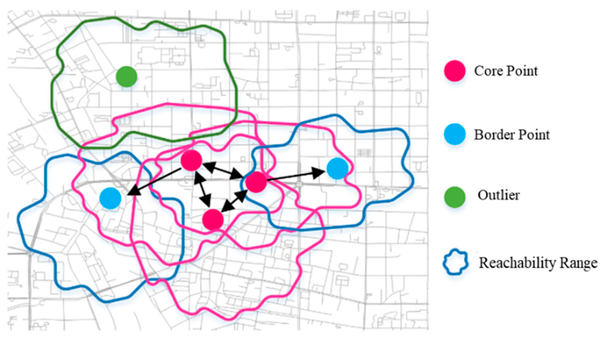
For the DBSCAN algorithm employed in this study, the two core parameters are clearly defined as follows: Epsilon ($\epsilon$) refers to the radius of the neighborhood around a given data point (i.e., the maximum distance within which other data points are considered neighbors of the target point); MinPts (Minimum Points) denotes the minimum number of data points that must exist within the $\epsilon$-neighborhood of a point for that point to be classified as a core point (a core point is the core of a cluster, around which a dense cluster can be formed). However, existing methods such as fixed-radius buffering fail to consider the influences of living environments and traffic patterns on human activity. To enhance DBSCAN’s urban applicability, we propose an improved algorithm with road network and transportation constraints, using flexible equal-distance or equal-time buffers to highlight regional and travel mode impacts on outbreak points. The clustering process (Figure 1) involves:

• Constructing a city graph from OSM road network data (nodes = intersections/endpoints, edges = road segments, weights = segment length);
• Mapping each patient point to the nearest road network node;
• Defining a search radius (for instance, distance or time). For a patient point, using accessibility analysis algorithm to calculate all reachable nodes within the radius;
• In DBSCAN’s core point judgment, two points are “density-reachable” neighbors if the mapped node of one lies within the reachable set of the other (i.e., real road network distance < radius). This avoids misclassifying points close in Euclidean distance but separated by rivers, walls, or highways, making clusters more realistic.

Module 3: Cluster Centroid Localization Fusing Spatiotemporal and Environmental Weights

Among the multiple clusters obtained via clustering, the largest cluster containing the most data points is selected, as it is deemed most likely to contain or be closest to the initial outbreak source. To calculate a representative outbreak point coordinate from this cluster, an improved Inverse Distance Weighting (IDW) interpolation method is adopted. For each point $p_i\left(x_i,y_i,t_i\right)$, within the cluster, its comprehensive weight $w_i$ consists of three components:

$$w_i={\displaystyle \frac{1}{{\displaystyle {\sum }_{j=1}^n}{d}_{ij}^{-2}}}\times {\tau }_i\times {\rho }_i$$

(8)

where, $d_{ij}$ is the Euclidean distance between point $p_i$ and other points $p_j$ within the cluster. The first term represents the standard IDW distance weight, assigning higher weights to points that are closer to other points. ${\tau }_i={\displaystyle \frac{1}{t_i-t_0+1}}$ is the temporal weight, where $t_i$ is the infection date of point $p_i$ and $t_0$ is the earliest infection date of the epidemic. This weight assigns higher weights to points with earlier infection times, consistent with the “earlier source” hypothesis. ${\rho }_i={\displaystyle \frac{P_i}{{\displaystyle {\sum }_{k=1}^n}{P}_k}}$ is the environmental weight, where $P_i$ is the total number of POIs within the road network reachable range R of point $p_i$. This weight characterizes the population aggregation potential of the point’s location; locations with greater potential foot traffic have a higher probability of being the outbreak source causing an aggregated epidemic.

Finally, the coordinates $\left(X,Y\right)$ of the estimated outbreak centroid are calculated as the weighted average of all points:

The final estimated outbreak point coordinate is the weighted average of all cluster points:

$$X={\displaystyle \frac{{\displaystyle {\sum }_{i=1}^n}(w_i·x_i)}{{\displaystyle {\sum }_{i=1}^n}{w}_i}}, Y={\displaystyle \frac{{\displaystyle {\sum }_{i=1}^n}(w_i·y_i)}{{\displaystyle {\sum }_{i=1}^n}{w}_i}}$$

(9)

In this method, SEAIR model calibration was performed by fitting the model to early-stage reported case data, with parameters optimized based on the coefficient of determination (R²) and goodness-of-fit measures. While this process inherently carries calibration uncertainty that may propagate to the T₀ estimate, the 3-sigma criterion provides an adjustable threshold, enabling iterative refinement. The framework is designed as an auxiliary decision-support tool that acknowledges and accommodates such errors, rather than claiming deterministic precision.

What’s more, The 3-sigma criterion was employed as an anomaly-detection threshold rather than an assumption of normality for the overall epidemic curve. Specifically, T₀ is identified as the first day when new cases exceed the mean plus three standard deviations of the pre-outbreak baseline, indicating a statistically significant onset of sustained transmission. This method, rooted in statistical process control (e.g., Shewhart charts), is a standard practice in infectious disease surveillance for detecting epidemic emergence and does not require the full case series to be normally distributed.

It should be noted that the DBSCAN clustering is applied to cases occurring from the first reported case up to T₀, rather than the full epidemic duration. Since T₀ (determined by the 3-sigma criterion) marks the transition to significant community transmission, cases within this early window are spatially limited and directly linked to the initial outbreak. Consequently, the largest cluster identified in this pre-T₀ period is assumed to contain the outbreak origin, as it represents the earliest and most concentrated transmission activity. Road-network distance was used for clustering to respect actual travel constraints. In contrast, Euclidean distance was applied in the IDW calculation to efficiently generate a continuous spatial attraction field, as the slight distance discrepancy at the 1.5 km grid scale does not substantially affect the weighting outcome.

2.3.2. Infectious Disease Diffusion Model Based on “Cell-Type” Living Structure Hypothesis

To balance data granularity and model accuracy, a diffusion model based on the “cell-type” living structure hypothesis is proposed. The core assumption is that under epidemic threats, population daily activity ranges contract spontaneously or due to policies into small, fixed ranges around residences or workplaces (“cell-type” movement). The model uses medium-granularity multi-source data to quantify regional attractiveness and simulate local diffusion for fine-grained spatiotemporal transmission simulation. It consists of two key parts: tensor CP decomposition-based regional attraction quantification and grid-space “cell-type” diffusion simulation.

Module 1: Regional Attraction Quantification Based on Tensor CP Decomposition

The goal is to generate a comprehensive matrix reflecting each spatial unit’s potential for population aggregation and viral transmission risk, providing a spatial weight field for simulation. This process has two stages: (a) using tensor CP decomposition to quantify differential impacts of POI categories; (b) fusing multi-source geographic data to generate a comprehensive attraction matrix.

(a)

POI Category Attraction Weight Calculation:

To analyze the differential impacts of various urban functions on the spatial distribution patterns of the epidemic, this paper introduces the CANDECOMP/PARAFAC (CP) tensor decomposition method. The name “CANDECOMP/PARAFAC” derives from two independent yet contemporaneous academic studies that proposed the identical multi-dimensional tensor decomposition technique in 1970: CANDECOMP (an abbreviation for “Canonical Decomposition”) was put forward by Harshman, while PARAFAC (short for “Parallel Factors”) was independently proposed by Carroll and Chang in the same year. Since the two methods are mathematically equivalent and achieve the same decomposition effect, the combined term “CANDECOMP/PARAFAC” (abbreviated as CP) has been widely adopted in academic research to refer to this classic tensor decomposition approach.

As a powerful multi-dimensional data analysis tool, CP tensor decomposition is specifically designed to handle high-dimensional tensor data, which can effectively capture the complex inherent relationships among multiple variables that are difficult to be revealed by traditional two-dimensional methods (e.g., matrix decomposition). Unlike matrix decomposition (such as principal component analysis) that only processes two-dimensional data (rows and columns), a tensor is a multi-dimensional extension of a matrix, and CP decomposition decomposes a high-order tensor into a sum of a series of rank-one tensors (also called “outer product tensors”). Each rank-one tensor corresponds to a latent feature that reflects the combined effect of all dimensions of the original tensor, enabling the extraction of hidden association patterns among multiple dimensions.

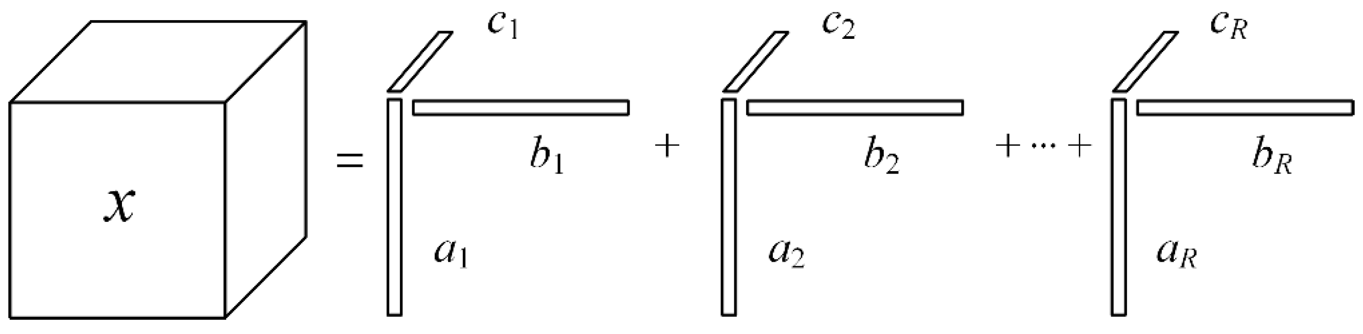
In the context of this study, where we need to explore the multi-dimensional relationships between geographic units, early patients, and POI categories (urban function types), CP tensor decomposition exhibits unique advantages. It can fully retain the multi-dimensional information of the original data (i.e., whether a certain POI category exists in a geographic grid associated with a specific patient) without losing key spatial and functional correlation information. By decomposing the constructed third-order tensor into rank-one tensors, CP decomposition helps us quantify the latent associations between each dimension: for example, the association strength between different geographic units and patient distribution, the correlation between POI categories (urban functions) and patient aggregation, and the hidden spatial patterns of epidemic spread related to urban functions. Figure 2 illustrates the CP decomposition process for a third-order tensor, clearly showing how the original tensor is decomposed into the sum of rank-one tensors to extract latent multi-dimensional relationships.

A third-order tensor is constructed to capture multi-dimensional associations between geographic units, patients, and POI categories. Dimensions represent: (i) geographic grid units in the study area, (ii) early patients, (iii) POI categories (e.g., catering/shopping, life services). Tensor elements $t_{ijk}=1$ if the k-th POI category exists in the i-th grid unit associated with the j-th patient, else 0. CP decomposition approximates the tensor as a sum of rank-one tensors:

$$\mathcal{T}\approx {\displaystyle \sum _{r=1}^R}{\mathbf{a}}_{\mathit{r}}\circ {\mathbf{b}}_{\mathit{r}}\circ {\mathbf{c}}_{\mathit{r}}$$

(10)

where $R$ is the tensor rank, ∘ is outer product. Among these factor matrices, the geographic unit factor matrix ${\mathbf{a}}_{\mathit{r}}$ (with dimensions of [number of geographic grid units × tensor rank R]) is specifically explained here to clarify its connotation and role in the study. Each row in ${\mathbf{a}}_{\mathit{r}}$ corresponds to one geographic grid unit (i.e., the i-th row corresponds to the i-th geographic grid unit in the study area), and each column corresponds to one rank component r. The element ${\mathbf{a}}_{\mathit{i}\mathit{r}}$ quantifies the strength of the association between the i-th geographic grid unit and the r-th latent feature (e.g., latent spatial patterns of epidemic aggregation related to specific urban functions). In other words, ${\mathbf{a}}_{\mathit{r}}$ characterizes the contribution of each geographic unit to different latent epidemic-related patterns: higher values of ${\mathbf{a}}_{\mathit{i}\mathit{r}}$ indicate that the i-th geographic grid unit has a stronger correlation with the r-th latent pattern, while lower values indicate a weaker correlation. This factor matrix effectively decomposes the spatial heterogeneity of geographic units, enabling the identification of key grid units that are closely associated with patient distribution and specific POI categories, and laying a foundation for quantifying the spatial coupling relationship between urban functions and epidemic aggregation. The POI category factor matrix ${\mathbf{c}}_{\mathit{r}}$ is key, with row vectors revealing the potential “attraction” or association strength of each POI category with patient spatial distribution patterns. Analyzing this quantifies the relative importance scores of POI categories in the epidemic environment, providing differentiated weights for multi-source data fusion.

The term ‘regional attraction’ should be interpreted as the environmental propensity for transmission, derived from the spatial coupling between case locations and POI distributions, rather than a direct measurement of real-time population flow. POI data serve as a static proxy for urban functional areas and routine human activity patterns. CP tensor decomposition is applied to uncover the latent relationships between the spatial attributes of case data and the surrounding POI environment, quantifying the relative risk of inter-location transmission. This method offers a pragmatic and computationally efficient solution for modeling disease spread in the absence of detailed mobility tracking data.

(b)

Multi-Source Geographic Data Layer Fusion for Comprehensive Attraction Matrix:

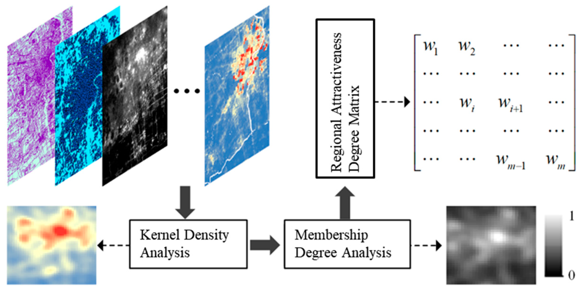
To obtain a spatially continuous attraction matrix, multi-source data (traffic flow, satellite remote sensing, population statistics, POIs) are fused. The process (Figure 3) includes:

• Data layer preparation: After unifying to WGS84, prepare layers: (1) weighted-sum POI kernel density (using category weights from CP decomposition), (2) population density kernel density (WorldPop), (3) nighttime light intensity kernel density (Luojia-1), (4) road network kernel density (OSM), (5) land use type (FROM-GLC, focusing on built-up areas).
• Kernel density analysis (KDE): Apply KDE to all continuous data layers with a bandwidth (search radius) matching daily activity radius. KDE is performed on each continuous data layer separately, with the search radius Rc (in km) serving as the bandwidth parameter of the kernel function.
• Fuzzy logic normalization: Normalize each layer’s KDE results to [0, 1] to eliminate dimensional differences.
• Weighted linear superposition: Superimpose normalized layers using equal weights (adjustable via expert scoring or AHP) to generate a comprehensive attraction matrix. Each element corresponds to a D_g km × D_g km grid’s comprehensive attraction value (higher = higher potential for population aggregation and transmission risk).

Module 2: Grid-Space “Cell-Type” Diffusion Simulation

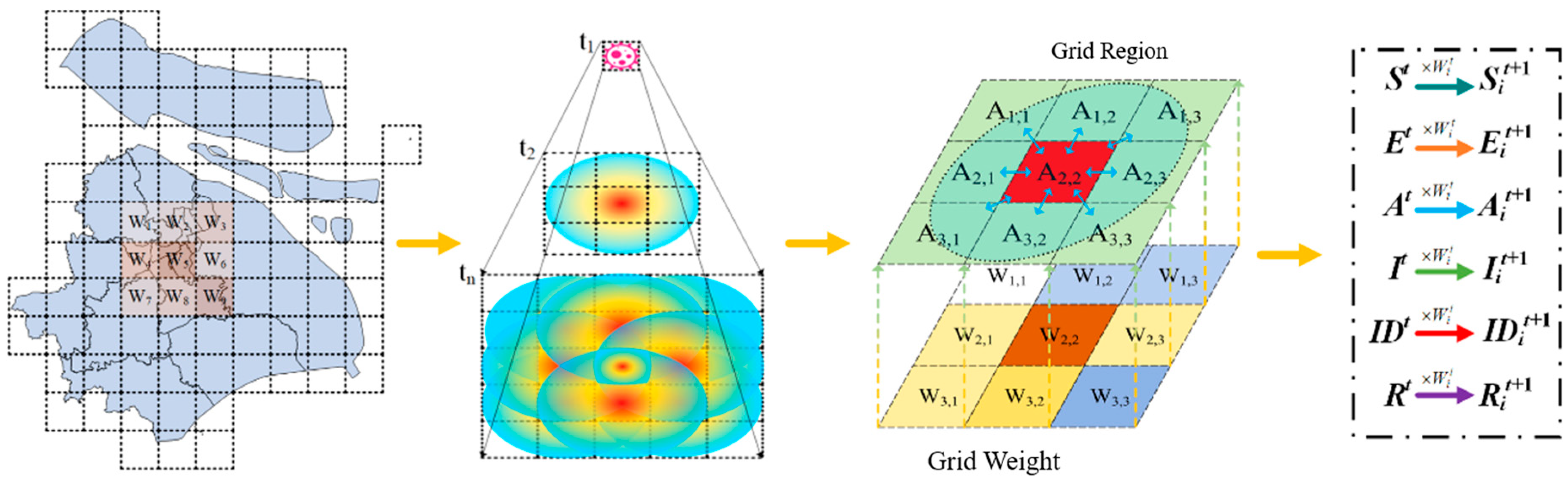
Using the estimated outbreak point as the initial transmission center, this step simulates viral diffusion in gridded space following “cell-type” logic (infected areas spread like cell division, daily expanding from existing centers to adjacent regions). The cellular diffusion process of infectious diseases is shown in Figure 4.

The cellular diffusion process includes:

(1)

Spatial discretization and initialization: The study area is divided into square cells, assuming uniform intra-cell infection risk and inter-cell transmission. The cell containing the estimated outbreak point is marked as the initial infected grid (day 1 transmission center), with initial infections set to the actual new cases that day. Although square grids may introduce minor directional bias, at proper resolution this discrepancy is negligible compared to reporting and mobility uncertainties. Moore neighborhoods partially compensate, square tessellations remain prevalent in CA-based epidemic models, and the POI-derived attraction field further reduces geometric artifacts.

(2)

Neighborhood diffusion and potential infected grid screening: Each current infected grid (transmission center) diffuses to its $R_c^2/D_g^2$ adjacent grids (Moore neighborhood) daily. For a transmission center, calculate the second quartile (Q2, median) of adjacent grids’ attraction values. A grid is marked as a potential infected grid for the next day only if its attraction value ≥ Q2 (assuming viruses spread more easily to high-attraction areas).

(3)

Infection number spatial allocation: Daily new infections (input from SEAIR predictions or actual reports) are allocated to potential infected grids via two-step weighted rules:

• Step 1 (allocation among transmission centers): Allocate total infections proportionally to each center’s attraction weight: $n_k=N_t\times {\displaystyle \frac{A_k}{\sum A_m}}$ ($N_t$ = total new infections; $A_k$ = attraction of center k; m = number of centers).
• Step 2 (allocation among potential grids of a center): Allocate each center’s $n_k$ proportionally to its potential grids’ attraction weights: $n_{kj}=n_k\times {\displaystyle \frac{A_{kj}}{\sum A_{kj}}}$ ($A_{kj}$ = attraction of grid j adjacent to center k).

If a grid is selected by multiple centers, its final infections are the sum of allocations. Grids with infections become new transmission centers the next day. Iterate daily until the simulation ends.

This model simulates localized transmission under control policies by introducing attraction-based grid screening, avoiding single-path limitations of tree models and allowing multiple dynamic transmission centers—more realistic for “multi-point spread” under lockdowns. It balances computational complexity and accuracy using accessible data (grid statistics, POIs, basic geography).

It should be noted that the proposed diffusion model is a spatially explicit framework designed to simulate the spatial propagation mechanism, rather than an endogenous epidemiological model that predicts case numbers. The daily infection count is provided as an external input to anchor the model to observed reality and avoid secondary errors from growth-rate estimation. The model then simulates the transmission process by spatially allocating these cases based on derived diffusion probabilities (e.g., network distance, attraction field). Thus, the core contribution lies in modeling where the virus spreads and why, serving as a spatial decision-support tool for outbreak source estimation and risk mapping.

For the attraction field, equal weights were assigned to POI categories due to unknown relative risks, and a median threshold was used for its robustness in delineating risk zones. Although these settings produced consistent results, we acknowledge that variations could influence outbreak location and diffusion patterns. The framework is adaptable, and a systematic multi-parameter sensitivity analysis is recommended for future research.

3. Results

3.1. Experimental Setup and Parameter Selection

To comprehensively evaluate the proposed framework, this section describes the experimental configuration, including the performance metrics and the rationale behind key parameter settings.

3.1.1. Performance Metrics

To quantitatively evaluate simulation accuracy, daily simulated infection grids were compared with actual reported patient residential locations, and two metrics were calculated: coverage rate (the proportion of actual patients falling within simulated grids) and precision rate (the proportion of simulated grids that actually contained patients).

This study primarily focused on the model’s capability to cover actual infected patients. Coverage rate is defined as the ratio of the number of patients covered by infection areas simulated by the model on day t ($N_c^t$) to the total number of actual infected patients on that day ($N_a^t$), as shown in Equation (11). The core purpose of this metric is to ensure that the simulated area encompasses as many actual infected patients as possible, thereby assessing the model’s ability to capture actual infection points.

$$P_c^t={\displaystyle \frac{N_c^t}{N_a^t}}$$

(11)

Precision rate measures the proportion of areas simulated by the model that are actually infected, specifically the ratio of the number of actually infected areas predicted by the model on day t($N_{pa}^t$) to the total number of simulated infection areas on that day ($N_{pre}^t$), as shown in Equation (12). This metric effectively evaluates the model’s performance in reducing false positives.

$$P_{pre}^t={\displaystyle \frac{N_{pa}^t}{N_{pre}^t}}$$

(12)

By synthesizing these two metrics, we can not only comprehensively evaluate the model’s effectiveness in covering actual infection areas but also ensure the accuracy of the model in avoiding the misclassification of non-infected areas as infected.

3.1.2. Parameter Selection

The selection of key spatial parameters—including the grid resolution D_g = 1.5 km, KDE bandwidth Rc = 5 km, DBSCAN settings (eps = 5 km, MinPts = 1), and attraction-field thresholds—was guided by empirical rules, prior studies, and the spatial characteristics of the study areas.

Grid resolution (1.5 km × 1.5 km): This resolution balances human activity scale (studies indicate a typical daily radius of 4–7 km, which covers approximately 30–35 grid cells at 1.5 km), statistical stability (avoiding the “small number problem” in overly fine grids), and input data quality constraints. It provides sufficient granularity for intra-urban heterogeneity while maintaining computational efficiency.

KDE bandwidth: The bandwidth was determined based on the spatial distribution of POIs to reflect meaningful local activity catchments, ensuring that the derived attraction field aligns with actual urban functional areas. Following the recommendations in [29], Rc is set within the range of 4–7 km.

DBSCAN parameters: The Epsilon parameter was set to 5 km, a value supported by urban mobility studies on daily activity radius, though it remains adjustable. MinPts was set to 1, reflecting the epidemiological principle that a single infected individual can initiate or propagate a transmission chain.

Attraction-field thresholds: Equal weights were initially assigned to different POI categories due to the lack of prior knowledge on relative transmission risks. A median threshold was adopted for risk zone delineation due to its robustness against outliers in the early-stage data.

The selection of the 1.5 km grid resolution was based on preliminary empirical testing in Wuhan, which compared 500 m, 1 km, 1.5 km, and 2 km resolutions. These preliminary tests indicated that 1.5 km provided a reasonable balance between spatial detail and statistical stability; however, the specific quantitative results from these tests are no longer available. Finer grids (e.g., 500 m or 1 km) tend to increase the number of candidate grids for case allocation, amplifying the randomness of spatial assignment and leading to overly dispersed infection patterns. Coarser grids (e.g., 2 km or above) reduce the number of candidate grids, resulting in more aggregated patterns akin to a “tree-like” population structure. The 1.5 km resolution preserves a degree of randomness while better reflecting the influence of population aggregation on transmission. It should be noted that a systematic quantitative validation across all study areas (Wuhan, Xi’an, Shanghai, and Hong Kong) was not performed within the scope of this work. Although the 1.5 km resolution yielded plausible simulation results consistent with the observed epidemic trends in Xi’an, Shanghai, and Hong Kong, we acknowledge that a multi-city sensitivity analysis is necessary to further validate the robustness of the chosen resolution, and we recommend this as future work.

3.2. Impact of Epidemic Prediction Accuracy on Early Stage Division and Data Screening

Taking Shanghai as an example, we explored the impact of using different lengths of initial data to fit the SEAIR model on prediction results and subsequent outbreak point estimation. Data from the first 10, 15, 20, and 40 days of the epidemic were used to fit the model, find approximate optimal parameters (

Table 3. Approximate Optimal Parameters of Shanghai SEAIR Model with Different Initial Data Lengths.

Days	E	A	I	β	θ	φ
10	3248.9970	66.7767	106.812	0.9033	0.0167	0.0307
15	2519.5694	31.2486	63.4667	0.9123	0.0637	1.79 × 10 −7
20	1902.192	125.7379	281.2181	0.9999	0.0667	0.0017
40	3445.1567	606.9305	954.0432	0.9984	0.0258	0.0081

), and extrapolate predictions.

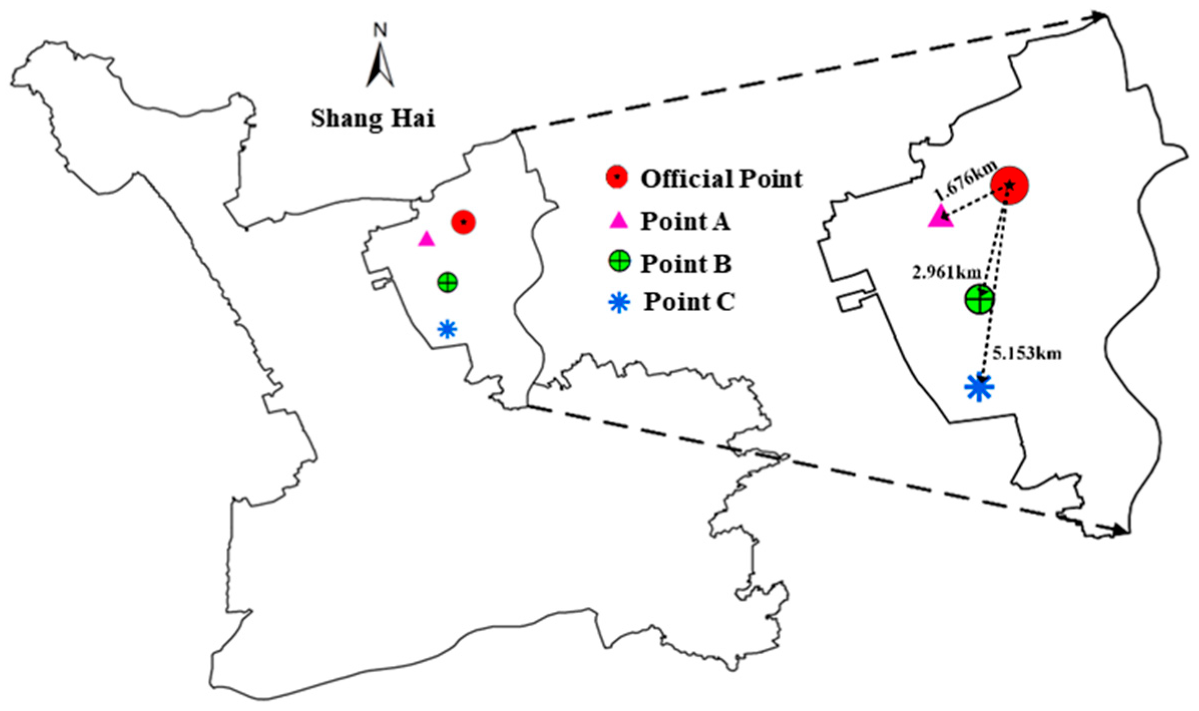
As data length increased, the coefficient of determination (R²) between predicted and actual curves improved, indicating better prediction accuracy. Applying the 3-Sigma criterion to each prediction yielded epidemic rapid rise start points of 5, 9, 13, and 16 days, respectively. Since detailed Shanghai patient residential data were only systematically published from 6 March 2022, only the 16-day (T₀ = 16) scheme could be evaluated. Figure 5 shows the comparison between the estimated outbreak points (for ease of description, hereinafter referred to as outbreak points C, B, and A) based on the 15-day (T₀ = 9), 20-day (T₀ = 13), and 40-day (T₀ = 16) forecast data and the officially announced outbreak point in [30]. All estimated points were southwest of the official point. Quantitatively, the 40-day scheme (closest to the official point, 1.676 km) outperformed 20-day (2.961 km) and 15-day (5.15 km) schemes. This demonstrates that prediction accuracy directly determines inflection point identification and the “purity” of early data, with more accurate predictions leading to more reliable outbreak point estimates.

3.3. Multi-City Outbreak Source Estimation Results and Comparative Analysis

Applying the full model to Xi’an, Shanghai, and Hong Kong. SEAIR model goodness-of-fit (R²) for Xi’an and Hong Kong epidemic time-series data was 0.945 and 0.873, respectively, indicating good trend capture. Optimal parameters are in

Table 4. SEAIR Model Optimal Parameters.

City	E	A	I	β	θ	φ
Xi’an	499.9991	77.2899	104.3007	1	0.0374	0.0262
Hong Kong	510.8527	43.8375	74.1575	1	0.0186	0.0469

.

Calculated T₀ values: Xi’an = 6 (14 December 2021, <14 days, due to early strict measures shortening the epidemic inflection point); Shanghai = 16 (16 March 2022, close to 14 days, due to late measures); Hong Kong = 31 (13 February 2022, >14 days, due to no strict measures and an incorrect epidemic start time selection).

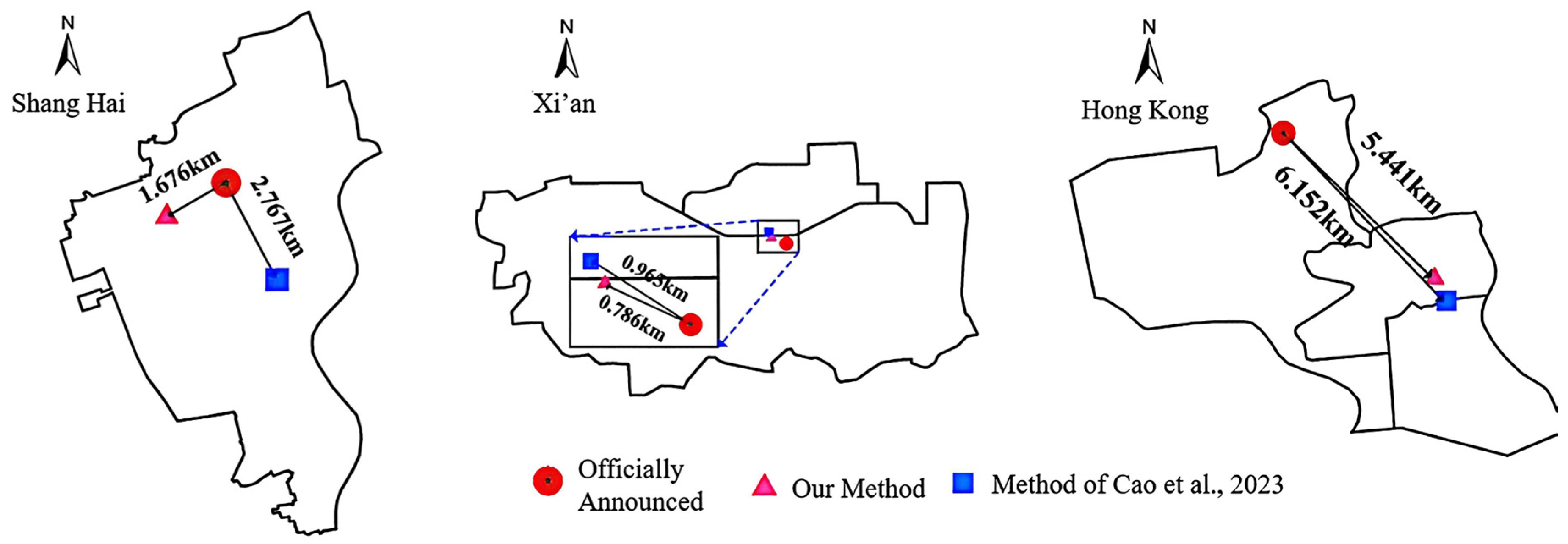
Figure 6 shows final outbreak point estimates for the three cities, along with officially traced locations (Xi’an: Chang’an University Family Compound, Yanta District [31]; Hong Kong: Kwai Chung Estate, Kwai Tsing District [32]) and estimates from reference [24]. Distances between our estimates and official points: Xi’an 0.786 km, Shanghai 1.676 km, Hong Kong 5.441 km—shorter by 179 m, 1091 m, and 711 m than reference [24], respectively. Spatially, our method’s Shanghai estimate (southwest of the official point) differed from reference [24] (southeast) due to road network-constrained clustering, which identified a strip-shaped cluster along road axes (more realistic than circular clusters from Euclidean distance).

3.4. Regional Attraction Quantification Results Analysis

Validating the tensor CP decomposition and multi-source fusion method using Shanghai and Hong Kong data:

• POI category importance:

  Table 5. Importance Scores of POI Categories in Shanghai and Hong Kong.

  POI Category	Shanghai	Hong Kong
  Catering/shopping	0.862	0.470
  Life services	0.402	0.213
  Residential communities	0.208	0.249
  Medical/education	0.183	0.262
  Leisure/entertainment	0.099	0.119
  Business offices	0.089	0.192
  Financial services	0.034	0.052

  shows CP decomposition results. “Catering/shopping” had the highest importance (Shanghai 0.862, Hong Kong 0.470), followed by “life services” (Shanghai 0.402) and “residential communities” (Shanghai 0.208; Hong Kong 0.249). “Business offices,” “leisure/entertainment,” and “financial services” had lower importance.
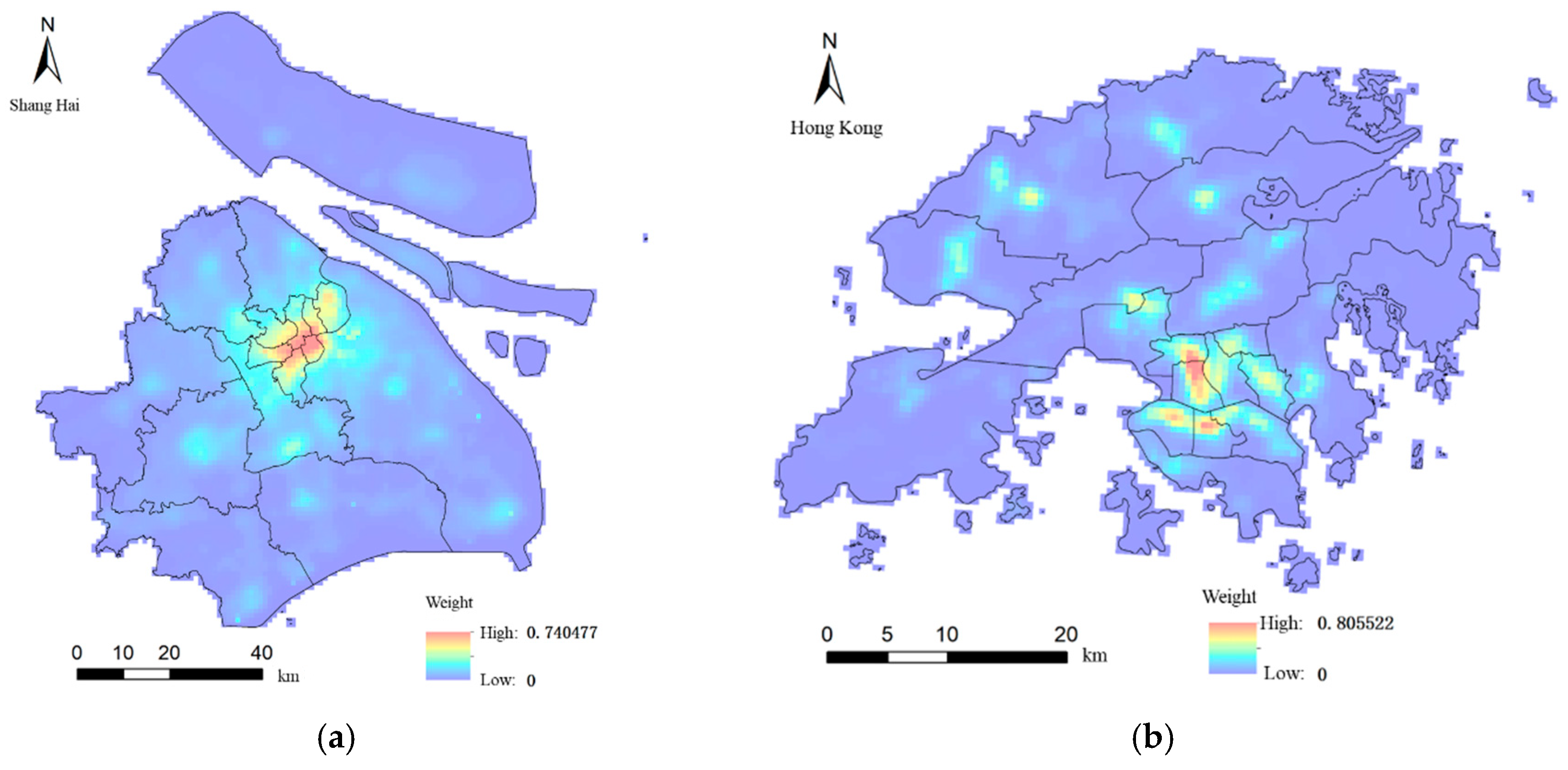
• Attraction spatial distribution: Figure 7 shows Shanghai’s high-attraction areas concentrated in city centers (Lujiazui, Xujiahui) with a “center-edge” pattern, while Hong Kong’s were more dispersed (Central, Causeway Bay, Tsim Sha Tsui) with peaks in islands and New Territories (e.g., near Disneyland). This reflects differences in urban planning and mobility patterns.
• Although the density of catering establishments in Hong Kong is higher than that in Shanghai, the faster pace of work and daily life in Hong Kong leads its residents to prefer individual meals and simple dining. Coupled with a lower proportion of dine-in customers in the local catering industry compared to Shanghai, the risk of clustered infections during dining is objectively reduced. In terms of population density, however, Hong Kong is significantly higher than Shanghai, which is particularly reflected in the much greater passenger density of public transportation. This results in more frequent human contact in public spaces, thereby increasing the probability of human-to-human transmission of respiratory infectious diseases. Consequently, for other types of points of interest (POIs), the overall risk of epidemic transmission in Hong Kong is higher than that in Shanghai.

3.5. Spatiotemporal Diffusion Simulation Process and Performance Evaluation

3.5.1. Spatiotemporal Diffusion Simulation

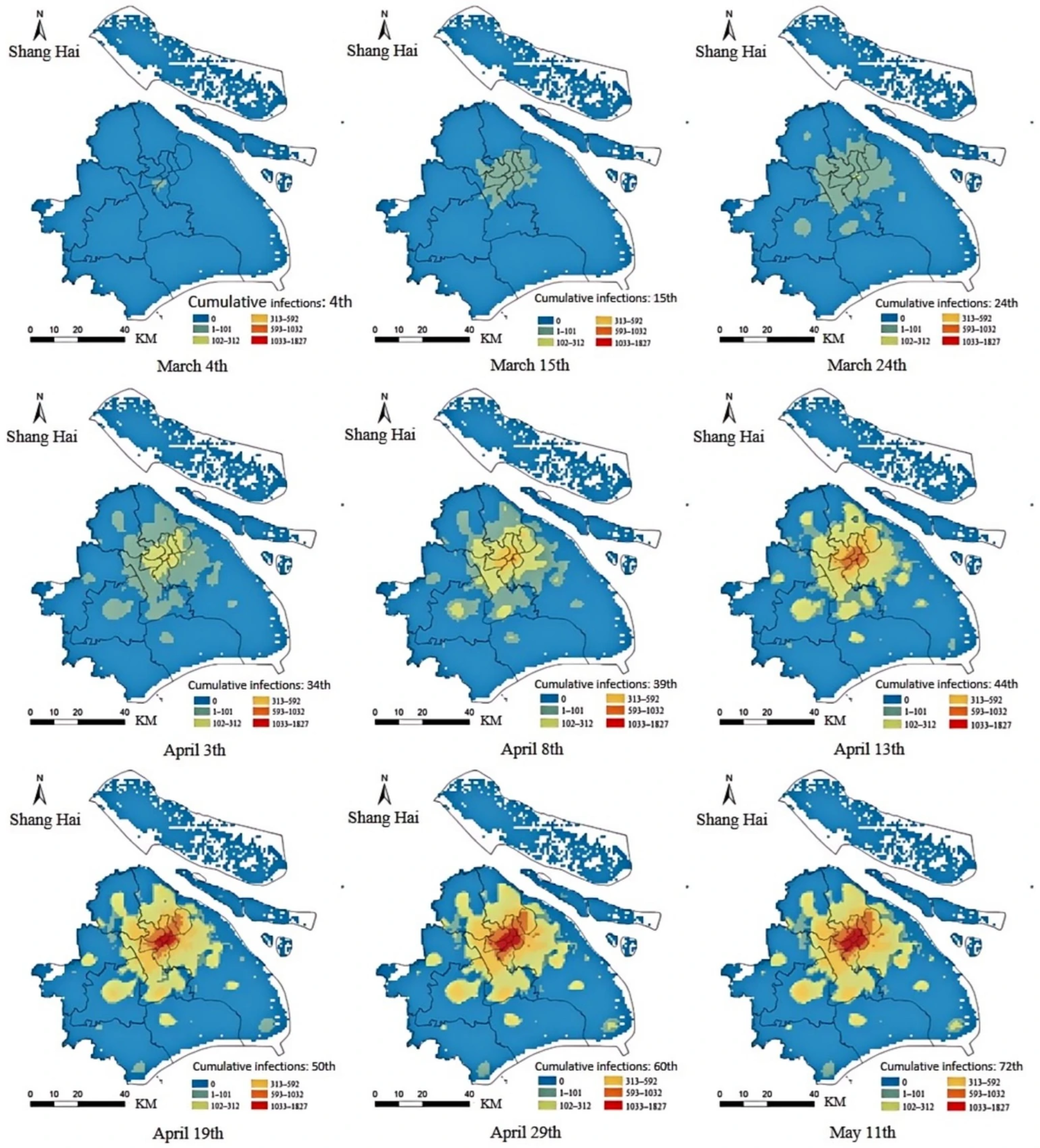
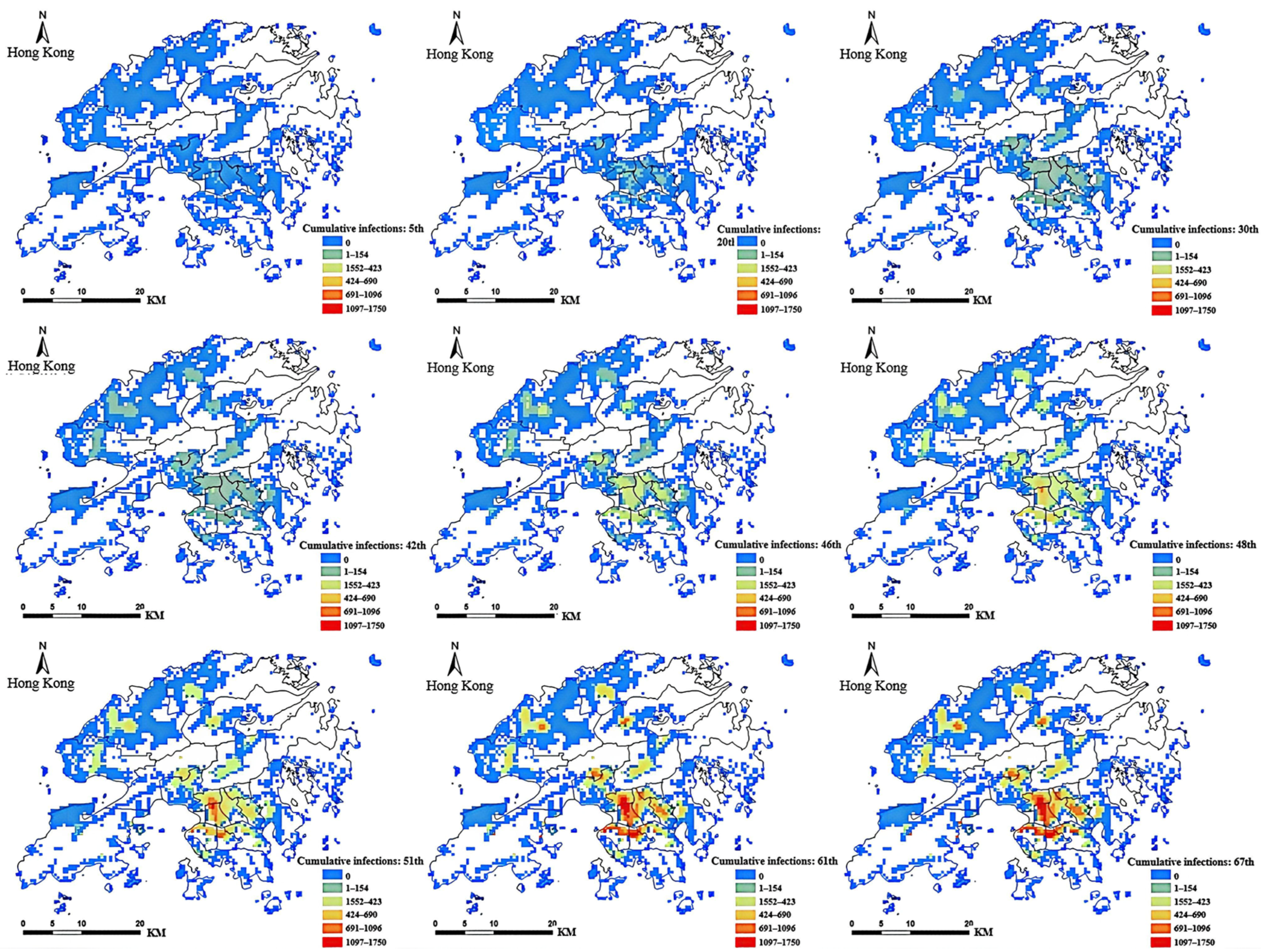
Using estimated outbreak points as initial centers, simulations were run for Shanghai and Hong Kong. Results (Figure 8 and Figure 9) use Jenks natural breaks classification to visualize infection density, with six levels (uninfected, Level 1: 1–101 cases, Level 2: 102–312, Level 3: 313–592, Level 4: 593–1032, Level 5: 1033–1827 for Shanghai; and uninfected, Level 1: 1–154 cases, Level 2: 155–423, Level 3: 424–690, Level 4: 691–1096, Level 5: 1097–1750 for Hong Kong).

• Shanghai: Simulation started near the intersection of Xuhui and Changning Districts. Early infections (e.g., 4 March 2022) were concentrated around the initial point, then spread along high-attraction directions, forming multiple secondary centers (reproducing real “multi-point spread”). By 13 April 2022, 22.9% of grids were infected, with slowing new infections post-control measures.
• Hong Kong: Simulation started near Kwai Chung Estate, Yau Tsim Mong. Early infections were concentrated, but due to dispersed high-attraction areas, spread was multi-point from the start.

3.5.2. Spatiotemporal Diffusion Performance Evaluation

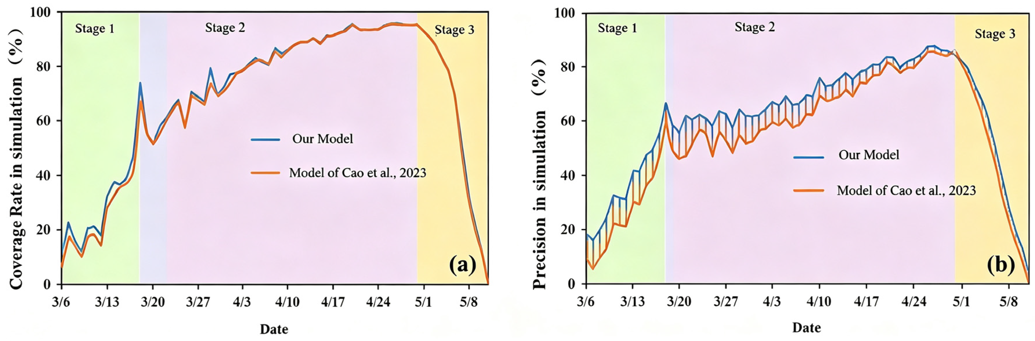
Figure 10 compares the accuracy variations between the method proposed in this paper and the method from reference [24] throughout the entire Shanghai simulation period (6 March 2022–11 May 2022). The entire cycle can be divided into three stages: a period of rapid accuracy increase (6 March 2022–18 March 2022), a period of slow growth and stability (19 March 2022–30 April 2022), and a period of declining accuracy (1 May 2022–11 May 2022). The precision rate of the method proposed was significantly higher than that of the comparative method in the early and middle stages (particularly during most of the first and second stages). Over the entire simulation period, the average coverage rate of the proposed method was 67.32%, with an average precision rate of 60.67%.

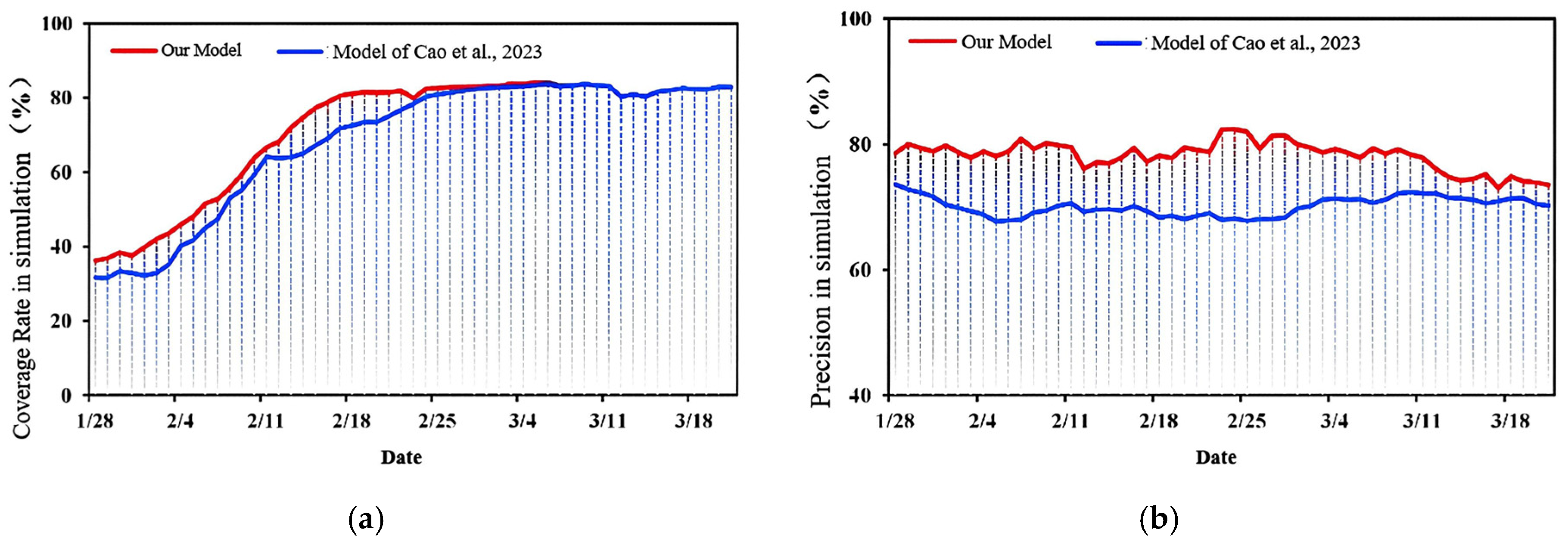
Figure 11 presents the simulation results of infection areas for the COVID-19 epidemic in Hong Kong from 28 January 20 to 28 March 2022, comparing the method in this paper with that of reference [24]. The results indicate that the method proposed here also performed robustly, achieving average coverage and precision rates of 72.9% and 78.84%, respectively, which were overall superior to the comparative method. This suggests that the “cell-type” diffusion hypothesis and the attractiveness-based allocation rules are effective when simulating epidemic stages characterized by localized, small-scale transmission under lockdown conditions.

4. Discussion

The integrated model constructed in this study, through empirical validation using COVID-19 cluster outbreak cases in three Chinese megacities, demonstrates its practical value and advanced capabilities in estimating early outbreak points and simulating spatiotemporal diffusion. The accuracy of the estimation results is closely related to several factors. First, the quality of epidemic prediction data is fundamental; longer initial data periods help obtain more stable SEAIR model parameters and a more accurate T₀ point. Second, the granularity and completeness of patient contact tracing data are crucial. Xi’an achieved the highest estimation accuracy (0.786 km), largely benefiting from its detailed published trajectory points and rich spatiotemporal information, while Shanghai and Hong Kong mainly provided residential address information, which naturally limited spatial accuracy. Finally, the impact of urban spatial structure cannot be ignored. This study employed road network-constrained clustering to make the results more realistic, a point particularly evident in the comparison of the Shanghai case. However, model performance is disturbed by a series of potential uncertainties or “disinformation” that must be carefully considered during application. These factors mainly arise from four aspects.

• Inherent limitations of the infectious disease dynamics model: As a simplified mathematical abstraction of complex transmission processes, the SEAIR model’s assumptions (e.g., homogeneous mixing, constant parameters) deviate from reality. Prediction errors directly propagate to the judgment of T₀. If the T₀ point deviates excessively, the selected “early data” may actually include cases from secondary or even tertiary transmission, thereby shifting the estimation focus to incorrect cluster areas.
• Uncertainty in the virus incubation period: For simplicity, this study adopted a uniform 14-day incubation period for retrospective time window calculations across all cases. In reality, the incubation period varies among individuals and changes with viral mutations (e.g., the shortened incubation period of the Omicron variant). Inaccurate incubation period estimates lead to deviations in the starting point of the time window, potentially missing true early cases or including too many non-early cases.
• Complexity of early population mobility patterns: The 3-Sigma criterion aims to filter out abnormal population flows caused by panic or policy guidance following a large-scale outbreak. However, during the initial “spark period” of the outbreak, the activities of early infected individuals may themselves be scattered and random, not necessarily forming clear spatial clusters. Furthermore, routine mobility based on commuting, business, etc., still exists in the early stage, and these complex mobility patterns may cause early cases to present as “weak signals” spatially, making them difficult to effectively capture by clustering algorithms.
• Quality issues of contact tracing data: This is the most direct factor affecting accuracy. These include: (a) recall bias and missing information: patients may not accurately recall all their activity trajectories; (b) inconsistent data granularity: for example, Shanghai provided only residential addresses, failing to reflect other important exposure locations such as workplaces and shopping venues; (c) delayed or selective publication: not all case contact tracing information is released in a timely or complete manner; (d) geocoding errors: the process of converting addresses to geographic coordinates may introduce errors. These data-level noise and biases directly affect clustering and weight calculation.

Regarding diffusion simulation, the “cellular” model demonstrates high accuracy in the early and middle stages of the epidemic, with its advantage lying in capturing the localized characteristics of transmission under lockdown conditions. However, the decline in accuracy in the later stages of simulation suggests limitations of the model. First, the model does not account for long-distance “jump” transmission through public transportation, emergency travel, etc., which may emerge in the middle and late stages due to prevention and control gaps or special events (e.g., patient transfers). Second, the model allocates the daily number of new infections as an external input, failing to dynamically couple with the number of susceptible individuals within the grid, representing a relatively mechanical distribution that does not fully capture transmission dynamics. Finally, the construction of the attraction matrix relies on static POI and geographic data, unable to dynamically reflect the dramatic changes in population activity patterns caused by evolving prevention and control policies.

While this study endeavored to select auxiliary geospatial datasets proximate to the pandemic period (2021–2022), we acknowledge a temporal discrepancy between the study period and the acquisition years of Luojia-1A (13 June 2018, WorldPop (2020 version), and FROM-GLC (2018 version). Furthermore, rigorous statistical validation of the temporal consistency of these datasets was not conducted. The potential implications of this temporal inconsistency for the attractiveness field and diffusion simulation are twofold: (1) nighttime light and population data may not fully reflect the actual population density distribution during the pandemic; and (2) land cover data may introduce inaccuracies in newly developed urban areas. Nevertheless, population density and fundamental geospatial data typically undergo only marginal changes within a two-year span. Additionally, the grid resolutions employed in this framework for spatial aggregation and tensor field decomposition both exceed 1 km, rendering the model relatively robust to minor temporal deviations in auxiliary data. Despite this robustness, caution is advised when interpreting results for rapidly urbanizing regions. Future work should prioritize the integration of auxiliary datasets that are temporally consistent with the specific event timeframe.

While the multi-city case studies provide initial validation for the proposed framework, we acknowledge that the current evaluation has several limitations. First, the evaluation is limited by the absence of a systematic quantitative comparison with baseline or alternative models (e.g., standard Euclidean-distance clustering, classical SEIR/CA diffusion models). Such a comparison would more rigorously demonstrate the model’s robustness and generalizability. A comprehensive benchmark against existing methods is therefore suggested for future research to further validate the spatial estimation accuracy and computational efficiency of the proposed approach. Second, a limitation of this study is the absence of a systematic quantitative sensitivity analysis for the key model parameters, including the 1.5 km grid resolution, KDE bandwidth, DBSCAN settings (eps, MinPts), and attraction-field thresholds. Although these parameters were selected based on empirical rules, prior studies, and the spatial characteristics of the study areas, variations in these settings could influence the accuracy of outbreak source estimation and the spatial patterns of the diffusion simulation. For instance, changes in grid resolution may alter the randomness or aggregation of case allocation; adjustments to KDE bandwidth can modify the spatial extent of the attraction field; variations in DBSCAN parameters may affect the identification of the initial transmission cluster; and different threshold choices can lead to distinct risk zone delineations. While the framework is designed as an auxiliary decision-support tool and the parameter choices are well-founded, users should be aware of the potential impact of parameter configurations. Future work will focus on addressing these gaps by conducting comprehensive multi-parameter sensitivity analyses and benchmark comparisons to further validate model robustness across diverse settings.

5. Conclusions

To address precise source tracing and diffusion simulation for aggregated epidemics, this paper proposes an innovative integrated spatiotemporal model framework and validates it with multi-case studies. Key innovations include: (1) a two-stage framework linking outbreak point estimation and diffusion simulation; (2) an outbreak point estimation method fusing SEAIR, 3-Sigma, road network DBSCAN, and spatiotemporal-environmental weights; (3) a “cell-type” diffusion model with tensor CP decomposition-based attraction quantification.

Results show the outbreak point estimation method effectively locates initial transmission centers (distances: 0.786 km in Xi’an, 1.676 km in Shanghai, 5.441 km in Hong Kong), outperforming existing methods. The spatiotemporal diffusion model simulates urban transmission well, with coverage rates exceeding 90% in mid-stages (18% higher accuracy than related studies). Although COVID-19 mortality has decreased, scientific prevention remains vital. This research provides references for governments to deploy hierarchical control measures, optimize resource allocation, and curb transmission.

Future research directions: (1) Incorporate fine-grained dynamic mobility data (e.g., mobile signaling, bus cards) to calibrate the diffusion model and simulate “jump spread”; (2) Fuse deep learning with mechanistic models to enhance nonlinear transmission prediction; (3) Extend the model to other contact/respiratory infectious diseases (e.g., influenza, norovirus); (4) Optimize visualization system interactivity for decision support.

References

1. World Health Organization. Managing Epidemics: Key Facts About Major Deadly Diseases; WHO Press: Geneva, Switzerland, 2018. [Google Scholar]
2. National Health Commission of the People’s Republic of China. COVID-19 Prevention and Control Protocol, 8th ed.; Comprehensive Group of the Joint Prevention and Control Mechanism of the State Council for Responding to the COVID-19 Pandemic: Beijing, China, 2021.
3. Liu, Y.; Gayle, A.A.; Wilder-Smith, A.; Rocklöv, J. The reproductive number of COVID-19 is higher compared to SARS coronavirus. J. Travel Med. 2020, 27, taaa021. [Google Scholar] [CrossRef] [Scilit] [PubMed]
4. Kraemer, M.U.G.; Yang, C.H.; Gutierrez, B.; Wu, C.H.; Klein, B.; Pigott, D.M.; Open COVID-19 Data Working Group; Du Plessis, L.; Faria, N.R.; Li, R.; et al. The effect of human mobility and control measures on the COVID-19 epidemic in China. Science 2020, 368, 493–497. [Google Scholar]
5. Ferguson, N.M.; Laydon, D.; Nedjati-Gilani, G.; Imai, N.; Ainslie, K.; Baguelin, M.; Bhatia, S.; Boonyasiri, A.; Cucunubá, Z.; Cuomo-Dannenburg, G.; et al. Impact of Non-Pharmaceutical Interventions (NPIs) to Reduce COVID-19 Mortality and Healthcare Demand; Imperial College London: London, UK, 2020. [Google Scholar]
6. Vespignani, A.; Tian, H.; Dye, C.; Lloyd-Smith, J.O.; Eggo, R.M.; Shrestha, M.; Scarpino, S.V.; Gutierrez, B.; Kraemer, M.U.; Wu, J.; et al. Modelling COVID-19. Nat. Rev. Phys. 2020, 2, 279–281. [Google Scholar] [PubMed]
7. Kermack, W.O.; McKendrick, A.G. A contribution to the mathematical theory of epidemics. Proc. R. Soc. London. Ser. A 1927, 115, 700–721. [Google Scholar] [CrossRef] [Scilit]
8. Sirakoulis, G.C.; Karafyllidis, I.; Thanailakis, A. A cellular automaton model for the effects of population movement and vaccination on epidemic propagation. Ecol. Model. 2000, 133, 209–223. [Google Scholar] [CrossRef] [Scilit]
9. Pastor-Satorras, R.; Castellano, C.; Van Mieghem, P.; Vespignani, A. Epidemic processes in complex networks. Rev. Mod. Phys. 2015, 87, 925–979. [Google Scholar] [CrossRef] [Scilit]
10. Ajelli, M.; Gonçalves, B.; Balcan, D.; Colizza, V.; Hu, H.; Ramasco, J.J.; Merler, S.; Vespignani, A. Comparing large-scale computational approaches to epidemic modeling: Agent-based versus structured metapopulation models. BMC Infect. Dis. 2010, 10, 190. [Google Scholar] [CrossRef] [Scilit] [PubMed]
11. Jia, J.S.; Lu, X.; Yuan, Y.; Xu, G.; Jia, J.; Christakis, N.A. Population flow drives spatio-temporal distribution of COVID-19 in China. Nature 2020, 582, 389–394. [Google Scholar] [CrossRef] [Scilit] [PubMed]
12. Chang, S.; Pierson, E.; Koh, P.W.; Gerardin, J.; Redbird, B.; Grusky, D.; Leskovec, J. Mobility network models of COVID-19 explain inequities and inform reopening. Nature 2021, 589, 82–87. [Google Scholar] [CrossRef] [Scilit] [PubMed]
13. Génois, M.; Barrat, A. Can co-location be used as a proxy for face-to-face contacts? EPJ Data Sci. 2018, 7, 11. [Google Scholar] [CrossRef] [Scilit]
14. Chen, X.; Liu, J.; Xu, L.; Li, J.; Zhang, W.; Liu, H. Construction of COVID-19 case activity knowledge graph: A case study of Zhengzhou City. Geomat. Inf. Sci. Wuhan Univ. 2020, 45, 816–825. (In Chinese) [Google Scholar]
15. Jiang, B.; You, X.; Li, K.; Zhou, X.; Wen, H. Interactive visual analysis of COVID-19 epidemic situation using geographic knowledge graph. Geomat. Inf. Sci. Wuhan Univ. 2020, 45, 836–845. (In Chinese) [Google Scholar]
16. Cao, N.; Shi, C.; Lin, S.; Lu, J.; Lin, Y.-R.; Lin, C.-Y. Targetvue: Visual analysis of anomalous user behaviors in online communication systems. IEEE Trans. Vis. Comput. Graph. 2015, 22, 280–289. [Google Scholar] [CrossRef] [Scilit] [PubMed]
17. Qu, H.; Chan, W.-Y.; Xu, A.; Chung, K.-L.; Lau, K.-H.; Guo, P. Visual analysis of the air pollution problem in Hong Kong. IEEE Trans. Vis. Comput. Graph. 2007, 13, 1408–1415. [Google Scholar] [CrossRef] [Scilit] [PubMed]
18. Abdollahi, M.; Behzadi, M. Spatial analysis of COVID-19 incidence and mortality in Africa: A geographically weighted regression approach. J. Geogr. Syst. 2022, 24, 567–592. [Google Scholar]
19. Silva, L.A.; Oliveira, M.P.; Santos, R.S. Socio-spatial inequalities and COVID-19 spread in Brazilian cities: A spatial regression analysis. J. Transp. Health 2023, 29, 101328. [Google Scholar]
20. Sarkar, S.; Islam, M.Z.; Hasan, M.Z. Spatial determinants of COVID-19 transmission in Bangladesh: Insights from spatial econometric models. Model. Earth Syst. Environ. 2021, 7, 1987–2002. [Google Scholar]
21. Norlund, P.; Arsanjani, J.J.; Passch, J.M. Spatio-Temporal COVID-19 Modeling: A Global Systematic Review of Data Integration, Equity, and Lessons for Pandemic Preparedness. Int. J. Environ. Res. Public Health 2026, 23, 627. [Google Scholar] [CrossRef] [Scilit] [PubMed]
22. Fang, Z. Thinking and challenges of crowd dynamics observation from the perspectives of pubic health and public security. Geomat. Inf. Sci. Wuhan Univ. 2020, 45, 1847–1856. [Google Scholar]
23. Gao, B.; Yang, Y.; Wang, X.; Li, Z.; Wang, J.; Liu, Y. Budget-constrained outbreak detection and tracking via evolutionary optimization in complex networks. Phys. Scr. 2026, 101, 045202. [Google Scholar] [CrossRef] [Scilit]
24. Cao, W.; Zhao, S.; Tong, X.; Dai, H.; Sun, J.; Xu, J.; Qiu, G.; Zhu, J.; Tian, Y. Spatial-temporal diffusion model of aggregated infectious diseases based on population life characteristics: A case study of COVID-19. Math. Biosci. Eng. 2023, 20, 13086–13112. [Google Scholar] [CrossRef] [Scilit] [PubMed]
25. Goldberg, D.W.; Wilson, J.P.; Knoblock, C.A.; Ritz, B.; Cockburn, M.G. An effective and efficient approach for manually improving geocoded data. Int. J. Health Geogr. 2008, 7, 60. [Google Scholar] [CrossRef] [Scilit] [PubMed]
26. Tyris, J.; Dwyer, G.; Parikh, K.; Gourishankar, A.; Patel, S. Geocoding and Geospatial Analysis: Transforming Addresses to Understand Communities and Health. Hosp. Pediatr. 2024, 14, 292–297. [Google Scholar] [CrossRef] [Scilit] [PubMed]
27. Kilic, B.; Bayrak, O.C.; Gülgen, F.; Gurturk, M.; Abay, P. Unveiling the impact of machine learning algorithms on the quality of online geocoding services: A case study using COVID-19 data. J. Geogr. Syst. 2024, 26, 601–622. [Google Scholar] [CrossRef] [Scilit]
28. Okuonghae, D.; Omame, A. Analysis of a mathematical model for COVID-19 population dynamics in Lagos, Nigeria. Chaos Solitons Fractals 2020, 139, 110032. [Google Scholar] [CrossRef] [Scilit] [PubMed]
29. Guo, L.; Yang, W.Q.; Bi, Y. Study on the Scale of Daily Life Units Based on Residents’ Travel Characteristics. In Proceedings of the 2016 China Urban Transportation Planning Annual Conference, Shenzhen, China, 15–16 April 2016; Urban Transportation Planning Academic Committee of China Society of Urban Planning: Beijing, China, 2016; pp. 1004–1015. (In Chinese) [Google Scholar]
30. Wikipedia. 2022 Shanghai COVID-19 Outbreak. 7 April 2022. Available online: https://en.wikipedia.org/wiki/2022_Shanghai_COVID-19_outbreak (accessed on 28 August 2023).
31. Qilu Evening News. Xi’an’s Epidemic Ends: How to Respond if COVID-19 Strikes Again? 24 January 2022. Available online: https://new.qq.com/rain/a/20220124A0AIWJ00 (accessed on 25 January 2022).
32. Li, N. How Is the COVID-19 Virus (Source Tracing) Progressing in Hong Kong? Is There Spillover Risk? 14 February 2022. Available online: https://news.sina.com.cn/c/2022-02-14/doc-ikyamrna0626730.shtml (accessed on 16 February 2022).
Figure 1. Schematic Diagram of Road Network-Constrained DBSCAN Clustering Process. (Single-headed arrows from core points to border points denote direct density reachability; double-headed arrows between core points denote density connectivity.)
Ijgi 15 00429 g001
Figure 2. The CP Decomposition Process for a Third-Order Tensor.
Ijgi 15 00429 g002
Figure 3. Schematic Diagram of Regional Attraction Matrix Calculation. (The distinction between solid and dashed arrows is purely stylistic and does not convey additional information).
Ijgi 15 00429 g003
Figure 4. Schematic Diagram of the Cellular Diffusion Process of Infectious Diseases. (The different colors of the arrows and dashed box are purely stylistic and does not convey additional information).
Ijgi 15 00429 g004
Figure 5. Estimated Outbreak Points of the Epidemic in Shanghai Under Different Time-Fitting Data.
Ijgi 15 00429 g005
Figure 6. Comparison of Estimated and Actual Outbreak Points in Shanghai, Xi’an, and Hong Kon g. (Red circles denote the officially reported outbreak point; pink triangles indicate the outbreak point estimated by our model; blue squares denote the estimates reported in reference [24]).
Ijgi 15 00429 g006
Figure 7. Analysis of Regional Attractiveness Results: (a) Shanghai; (b) Hong Kong.
Ijgi 15 00429 g007
Figure 8. Simulation Results of the Spatiotemporal Diffusion of COVID-19 in Shanghai at Different Time Points.
Ijgi 15 00429 g008
Figure 9. Simulation Results of the Spatiotemporal Diffusion of COVID-19 in Hong Kong at Different Time Points.
Ijgi 15 00429 g009
Figure 10. Curves of Validation Results for COVID-19 Infection Area Simulation in Shanghai by Different Models: (a) Curve of Infection Area Coverage Rate; (b) Curve of Infection Area Precision. (The blue curve shows the results obtained by our model; the orange-red curve shows the results reported in reference [24]).
Ijgi 15 00429 g010
Figure 11. Curves of Validation Results for COVID-19 Infection Area Simulation in Hong Kong by Different Models: (a) Curve of Infection Area Coverage Rate; (b) Curve of Infection Area Precision. (The red shows the results obtained by our model; the blue curve shows the results reported in reference [24]).
Ijgi 15 00429 g011