Simulating Sustainable County-Level Land Use by Integrating the Mechanical Equilibrium Model with the Multi-Objective Genetic Algorithm

Abstract

Multifunctional land use has gained increasing attention for reconciling societal (life function), economic (production function), and environmental (ecological function) development needs and addressing sustainable land use challenges in rapidly urbanizing regions. Consistent with mainstream international land use functions (LUFs), this study’s production-living-ecological (PLE) framework covers three key land functions, matching global research paradigms. To develop a sustainable county-level land use quantitative structure optimization model, this study innovatively integrates a mechanical equilibrium model with the multi-objective genetic algorithm (NSGA-II), overcoming the limitations of conventional qualitative production-living-ecological spaces (PLES) optimization. Furthermore, by establishing a mapping relationship between urbanization drivers and PLES functional evolution, it also enables structural optimization across urbanization subsystems. The optimization results indicate the following adjustment directions: southern coastal and southwestern counties require targeted population and socioeconomic urbanization improvements, while northern counties demand differentiated ecological urbanization regulation, and southeastern coastal areas should prioritize ecological protection. Most counties exhibit cropland and construction land expansion alongside woodland shrinkage, featuring expanded production and living spaces but contracted ecological functions. In contrast, certain counties achieve coordinated sustainability by eliminating inefficient construction land. This study operationalizes macroscopic PLE coordination into feasible quantitative strategies, enriching optimization methodologies and providing transferable insights for territorial spatial governance.

1. Introduction

As a non-renewable and fundamental resource, land serves as the essential foundation for human production and daily life. Human activities have vigorously promoted urbanization and social progress, yet they have also intensified the problems of land resource scarcity and unbalanced utilization [1,2,3]. China’s rapid urbanization, with the rate soaring from 16.20% in 1960 to 65.22% by 2022, has led to a reduction in arable and encroachment of ecological land in some areas [4,5]. Recent urbanization has also demonstrated increasingly complex characteristics, with some cities displaying paradoxical development trends. For instance, growing vacant land and underused infrastructure [6] reveal the prevalent coexistence of city-wide expansion and local shrinkage. Unchecked peri-urban sprawl and human–land mismatches create new obstacles to sustainable land use [7,8].

Against this backdrop, multifunctional land utilization has emerged as a potential pathway for addressing these challenges by reconciling the social (living function), economic (production function), and environmental (ecological function) developmental demands [9]. The concept of land use functions (LUFs) originated in developed Western countries. It encompasses the various utilities and services that a land unit offers, shaped by both its natural attributes and anthropogenic activities [10]. The land use multifunctionality discussed in this paper specifically refers to the production-living-ecological functions (PLEF). This PLE framework aligns with the internationally mainstream land use functions (LUF) system by categorizing land into three core functions: production (economic), living (social), and ecological (environmental). It is thus fully compatible and comparable with global studies in this field. The essential definition of these three types of functions is mainly derived from the differences in the types and quantities of products and services provided during the process of land use [11,12]. Specifically, land for production functions refers to the area used for agricultural, industrial and commercial activities to obtain products and supply services. Land for living functions is the area that provides carrying capacity and guarantees human settlement functions. In contrast, land for ecological functions is the area primarily dedicated to regulating, maintaining and safeguarding ecological security functions.

The academic community has carried out extensive research on the relationships between the “production-living-ecological” (PLE) functions of land use. The existing consensus is that the production function is the material basis of the PLE functions, providing support for the improvement of living quality and the maintenance of the ecological environment, but the strengthening of the production function will constrain the ecological function [13,14]. The living function is the goal of optimizing production and ecological functions, promoting the continuous improvement of the production function and the ecological function, but the expansion of the living function will also encroach upon the space for production and ecological functions. The ecological function is the natural condition for land to provide ecological products and services for humans and to maintain human survival. It is the prerequisite for the realization of production and living functions, and its improvement or deterioration directly affects the development and changes of production and living functions [15]. The PLE functions are interdependent and irreplaceable. The performance of a single function depends on the roles of the other two functions, and the lag of one function also affects the performance of the other two functions. Only when the PLE functions adapt to each other, match each other, and work together can the comprehensive benefits of land use be maximized. The unreasonable expansion of any single function will affect the balance and development of the PLE functions.

As a spatial carrier of land functions, “production–living–ecological spaces” (PLES) refer to a collection of land units with specific spatial boundaries and attributes divided based on the land’s dominant PLE functions. Production space is the land space dominated by the production function, living space is the land space dominated by the living function, and ecological space is the land space dominated by the ecological function [16]. Optimizing territorial spatial patterns and promoting the coordinated, sustainable development of regional multi-functions has long been a core theme in territorial governance and a central research focus across global geography, urban planning, and land use science. The “balanced allocation” of PLE functions in this study refers to the optimal functional coordination, which is highly consistent with the actual planning and policy goals at the national and local levels. The “non-optimal” state of the research benchmark is mainly defined as taking the current land use structure of the study area as the starting point, which often has problems such as the encroachment of a certain function (such as ecology) and significant conflicts between functions.

Scholars have conducted extensive research on the functional identification and evaluation of the “production-living-ecological” space (PLES) of land at different levels such as provinces, cities, and counties. At present, two mainstream approaches have been formed: The land use classification method is one of the most widely used methods. This method relies on the determination of the surface cover type and dominant use of the land unit to achieve the rapid classification of plot properties and core carrying functions [17,18]. Its core advantage is that it is intuitive to operate and easy to promote, suitable for regional-scale studies with a wide research scope and a large number of plots.

Another mainstream method is the indicator evaluation method, which indirectly quantifies the intensity and level of the realization of each function by constructing a multi-dimensional indicator system (such as grain yield, population density, and ecological service value) [19]. It can more finely depict the internal differences of functions, but it depends on data availability and the scientific setting of indicator weights. To deeply understand the interaction relationships between different functions, some studies have further introduced various analysis models, for example, using the coupling coordination model to evaluate the overall synergistic or trade-off state of the system [15] or using the niche model to identify the competitive potential and spatial conflict patterns between different functions [20].

It is particularly noteworthy that recent studies have introduced a mechanical equilibrium model, attempting to quantitatively depict the dynamic mechanism of trade-offs between the PLE functions [14,21], which provides a novel perspective for understanding the internal trade-off relationships within the system. The interaction of the PLE functions in territorial space is essentially a dynamic equilibrium process of “synergy-trade-off”. This characteristic has significant inherent logical consistency with the “equilibrium steady state and deviation state under multi-force coupling” in physics. The mechanical equilibrium model has a preliminary application basis in the study of land use multifunctional coordination. Zhang et al. [14], in a national grid-scale study of land use functions, abstracted economic, social, and ecological functions into three vector forces with angles of 2π/3 between them. By calculating the magnitude and direction of the resultant force using the mechanical equilibrium model, they systematically revealed the spatial pattern of trade-off/synergistic relationships of land use functions in China, becoming a typical application example of the model and providing a methodological reference for subsequent related research. Thereafter, Zhang et al. [21] introduced this model in the study of PLE function coordination in the Yellow River Basin and effectively identified different functional coordination types. Kang et al. [13] used this model in the synergy/trade-off analysis of PLE functions in Shanxi Province to accurately diagnose the functionally dominant areas and constraint areas, verifying the model’s applicability and reliability in regional-scale studies.

Existing research (including the application of the mechanistic equilibrium model) mostly focuses on the identification of PLS dysfunction (in this study, it specifically refers to the lack of functions, functional conflicts, functional inefficiency, and other problems in the three core PLE functions of land) or the ex-post evaluation and explanation of trade-off relationships. However, how to actively use this understanding of the system mechanism to optimize future land use allocation remains a methodological challenge. Therefore, an important starting point of this study is to try to combine the mechanistic equilibrium model that reveals the mechanism with a multi-objective optimization algorithm that can actively search for optimal solutions, so as to promote the expansion of the research from “description and interpretation” to “simulation and optimization”.

In recent years, computer optimization algorithms have gradually been integrated into land resource allocation and land use optimization research [22,23,24]. Existing studies demonstrate the superior performance of NSGA-II in addressing land use optimization problems [25]. Current land use planning research typically employs direct optimization of the NSGA-II algorithm, focusing mainly on improvements to crossover-mutation operators, with limited coupling to other models [26,27]. For instance, Cao et al. [28] developed a crossover-mutation mechanism based on predefined patch characteristics, achieving optimization through exchanging adjacent patch land use types or randomly adjusting internal land category configurations. Wang et al. [29] proposed a mutation operation method using 3 × 3 grid cells, while Song & Chen [25] specifically focused on crossover operations for boundary units (those adjacent to different land types).

With the growing emphasis on sustainability, research has shifted from purely maximizing economic returns to coordinating multiple objectives: economic, ecological, carbon-related and social goals. This research trend has evolved along two main directions: algorithmic improvement and model coupling. On the algorithmic front, Huang et al. [30] proposed a fuzzy expert system-enhanced NSGA-II (Fuzzy-Expert-NSGA-II), which embeds expert rules, a hybrid adaptive neighborhood search and fuzzy membership functions. This approach effectively addresses the complex constraints and inherent uncertainties embedded in the optimization of agricultural planting strategies. In terms of model coupling, a body of studies combine NSGA-II with ecosystem service evaluation models. Dong et al. [31] coupled the InVEST model with NSGA-II for green infrastructure planning, taking habitat quality, grain yield and runoff reduction as targets to realize a multifunctional spatial layout. Liu et al. [32] explored trade-offs among various ecosystem services and adopted NSGA-II to screen Pareto-optimal solutions for water provision, water purification and carbon sequestration. Yang et al. [33] constructed a dual-scale multi-objective land allocation (DOLA) model by integrating ideal-point linear programming with NSGA-II, realizing the coordinated optimization of carbon emission patterns from both structural and spatial perspectives.

Other studies couple NSGA-II with spatial simulation models. Luan et al. [34] established an analytical framework integrating NSGA-II and the PLUS model to systematically optimize land use with the dual objective of maximizing economic and ecological benefits. Gu et al. [35] further coupled NSGA-II with PLUS under four carbon neutrality scenarios, natural development, low-carbon emission, high carbon storage and carbon neutrality, so as to simultaneously promote economic growth, reduce pollutant emissions and elevate carbon storage capacity. Collectively, these existing studies demonstrate that NSGA-II and its coupled improved versions can well resolve multi-objective conflicts in land use, providing solid quantitative support for regional sustainable development. Nevertheless, most coupled models merely serve as simulation tools and seldom couple the internal driving mechanisms with the optimization capability of the NSGA-II algorithm itself.

As the core driving force shaping the functional evolution of the PLES [36,37], urbanization has a decisive impact on the synergy of the PLE functions of land use and is a key factor for achieving regional sustainable development [38,39]. For a long time, the interaction between urbanization and land use has been an important topic in academic research. Existing studies indicate that evolving urbanization goals across different developmental stages drive marked shifts in land use structure [40,41,42]. This adjustment essentially reflects the adaptive changes of the land carrying functions during the urbanization process [43,44]. The so-called land carrying functions refer to the inherent attributes and ability of land, as a limited natural resource, to continuously meet various human needs. Its core lies in the land’s inherent endowment and potential regarding “what can be provided” and “how much can be sustained”. The diversified demands on land use patterns at different stages of urbanization have promoted the gradual multidimensional development of land use functions [45]. At the same time, the deepening of urbanization significantly affects the dynamic balance of the land use systems [46,47,48]. It should be noted that the land use systems refer to the specific management and utilization methods implemented by humans based on the land’s carrying functions.

In general, existing studies have well applied land use classification and indicator evaluation methods to identify and assess PLES functions and have used various analytical models to systematically diagnose trade-offs and synergies among these functions. These efforts have deepened our understanding of land use multifunctionality and provided effective analytical tools for planning practice. However, despite the solid foundation laid by previous research, two key issues remain to be addressed. First, there is a lack of a quantitative pathway to translate policy goals into land use allocation. The macro-level objective of “PLE functional coordination” largely remains at a qualitative stage, lacking a systematic and quantitative approach to convert it into actionable land use quantity optimization. Second, the integration of urbanization feedback is insufficient. Although urbanization is widely recognized as a core driver of land use function evolution, few studies have established a mapping relationship between urbanization subsystems and PLE functions within an optimization framework.

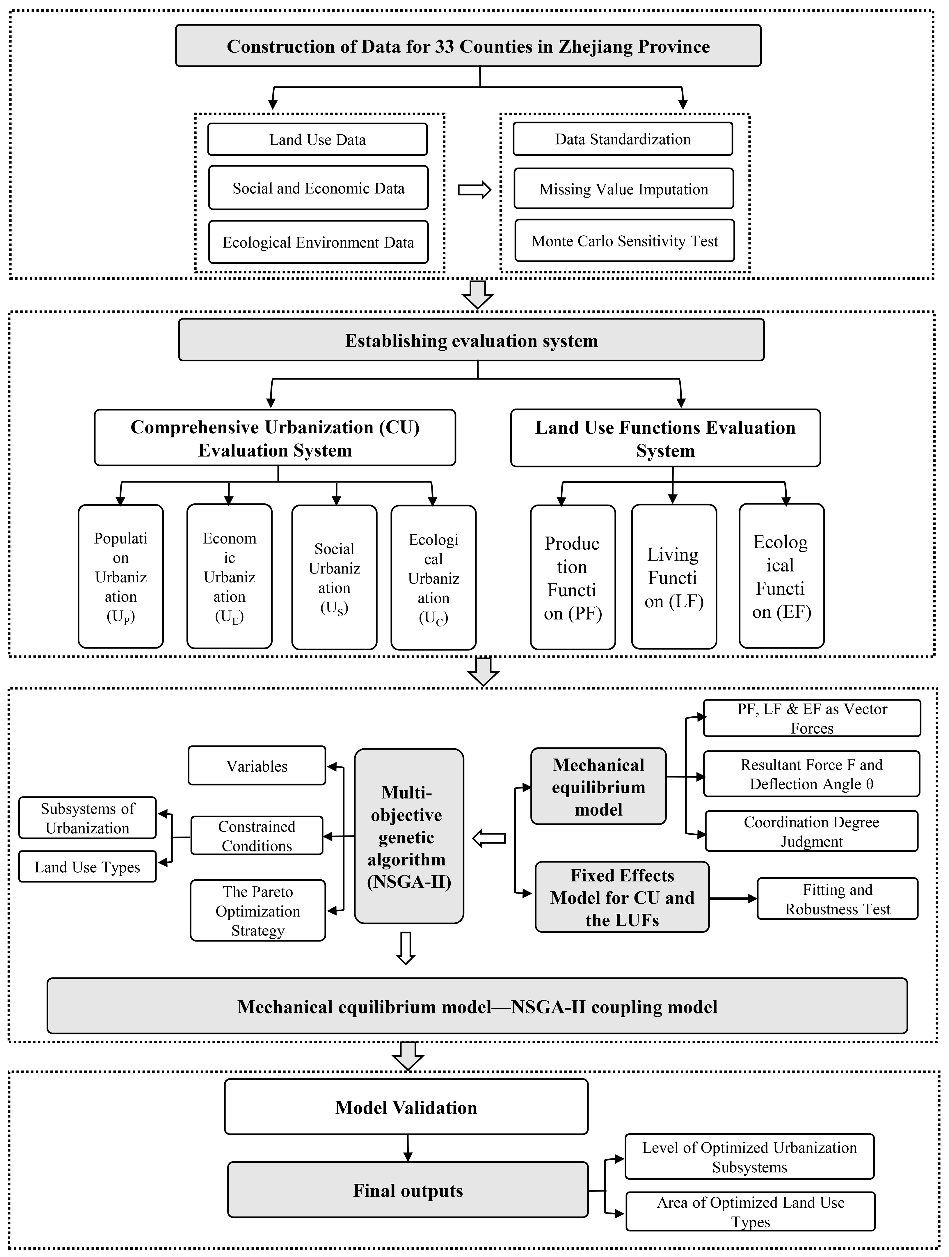
To address these gaps, this study for the first time couples a mechanical equilibrium model—capable of characterizing intrinsic system interactions—with the NSGA-II multi-objective optimization algorithm, shifting the research from “diagnosis” to “optimization” and establishing a systematic transformation pathway from the qualitative policy goal of PLE functional coordination to quantitative land use structure optimization. Furthermore, we use fixed-effects panel regression to construct a quantitative mapping between urbanization indicators and PLE function evolution, enabling coordinated regulation of demographic, economic, social, and ecological subsystems. This aims to provide a novel decision support tool for territorial spatial planning that is both theoretically grounded and practically operable (see Figure 1 for the technical framework).

2. Materials and Methods

2.1. Case Study

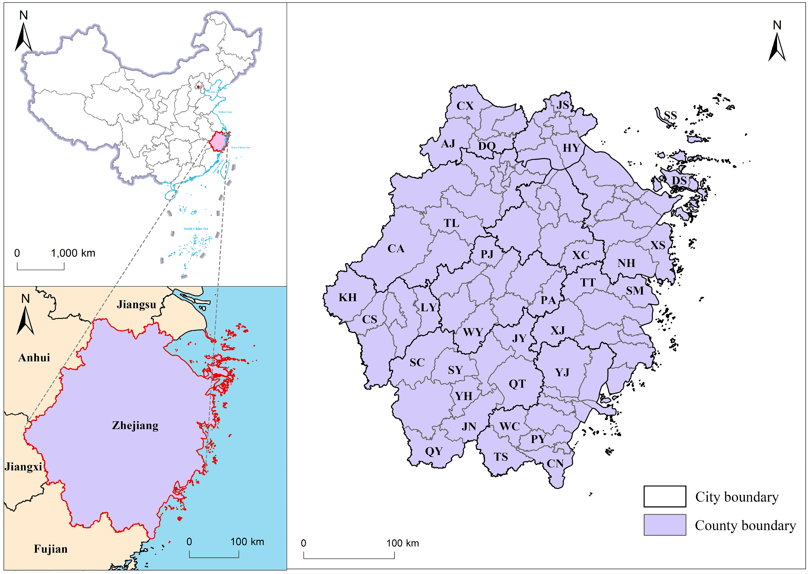
Situated along China’s southeastern coast, Zhejiang Province (118°01′–123°10′ E, 27°06′–31°11′ N) is a pivotal economic, cultural and transportation hub comprising 11 major cities: Hangzhou, Ningbo, Wenzhou, Shaoxing, Taizhou, Huzhou, Jiaxing, Jinhua, Quzhou, Zhoushan and Lishui (

Table 1. List of narrowly defined counties in Zhejiang Province.

Region	Prefecture-Level City	County (Abbreviation)
Eastern coastal	Ningbo	XS, NH
	Shaoxing	XS
	Zhoushan	DS, SS
Southern coastal	Wenzhou	YJ, PY, CN, WC, TS
	Taizhou	SM, TT, XJ
Central-western	Jinhua	WY, PJ, PA
	Quzhou	CS, KH, LY
Southwestern	Lishui	QT, JY, SC, SY, YH, QY, JN
Northern	Hangzhou	TL, CA
	Jiaxing	JS, HY
	Huzhou	DQ, CX, AJ

Note: The complete list of county names is provided in the Appendix A.

and Figure 2). In 2021, it represented 4.1% of China’s population and generated a substantial regional GDP of 6.5 trillion yuan, a testament to its national economic importance [49]. This study specifically examines county-level units in Zhejiang. While the general county concept includes counties, autonomous counties, municipal districts and county-level cities, the latter two categories exhibit distinct characteristics, where municipal districts feature low rural proportions and unstable administrative boundaries. County-level cities, however, are primarily upgraded from developed counties. These differences create challenges for long-term monitoring and cross-regional comparisons. Hence, adopting a narrow definition of counties, this research focuses on 33 representative county-level units (32 counties and 1 autonomous county) as research subjects (Table 1). This selection covers both sample representativeness and data comparability.

2.2. Data Acquisition

This study compiled the land use data from the 30 m resolution raster datasets (for the years 2000, 2005, 2008, 2010, 2015, 2018, and 2020) provided by the Institute of Geographic Sciences and Natural Resources Research (IGSNRR), Chinese Academy of Sciences (RESDC). Socioeconomic data were primarily sourced from the Zhejiang Statistical Yearbooks, as well as statistical yearbooks and government statistical bulletins of various cities, counties, and districts during the 2000–2020 period. For occasional missing data, linear interpolation served to ensure data completeness.

To ensure appropriate application of the proposed framework, explicit boundary conditions for input data are established. The Monte Carlo sensitivity analysis (with Gaussian error distribution) reveals that the interpolation-driven parameter fluctuations remain within ±2.3–4.5% (95% CI), provided that the missing data ratio does not exceed the historical variance structure observed in this study. Crucially, this framework is exclusively designed for county-scale macro-structural optimization rather than micro-parcel simulation. Researchers should refrain from applying this model when the fine-grid land use heterogeneity dominates the study objective, or when missing data imputation reverses the sign of core regression coefficients. These thresholds collectively define the valid applicability domain of our methodology.

3. Methodology

3.1. Establishing Evaluation System

3.1.1. Comprehensive Urbanization (CU) Evaluation System

Urbanization represents a complex, multidimensional process characterized by long-term evolution and dynamic development [50]. Compared with single indicators, comprehensive indicator systems more effectively capture the diverse characteristics and multifaceted nature of urbanization [51,52]. Building upon existing research findings [53,54,55], this study develops a comprehensive evaluation index system incorporating four dimensions—demographic, social, economic, and ecological urbanization—to provide a more systematic and holistic representation of urbanization’s multidimensional attributes (

Table 2. Urbanization evaluation system including population, economic, social and ecological dimensions.

Target Layer	Criteria Layer	Index Layer	Unit	Direction	Weight
CU	Population urbanization (UP)	Proportion of urban population	%	+	0.0515
		Population density	capita/km2	+	0.07294
		Proportion of employees in secondary and tertiary	%	+	0.01839
	Economic urbanization (UE)	GDP per capita	Yuan/capita	+	0.07327
		Proportion of output value of secondary and tertiary industries to GDP	%	+	0.01839
		Public budget revenue	Yuan/capita	+	0.10682
		Year-end balance of household savings deposits per capita	104 yuan/capita	+	0.1013
		Disposable income per urban resident	Yuan/capita	+	0.06012
	Social urbanization (US)	Total retail sales of consumer goods	Yuan/capita	+	0.07082
		Urban built-up area per capita	m2/capita	+	0.04583
		Paved road area per capita	m2/capita	+	0.06552
		Number of hospital beds	n/10,000p	+	0.04982
		Number of social welfare beds	n/10,000p	+	0.06333
		Number of full-time teachers in primary and secondary schools	n/10,000p	+	0.04228
	Ecological urbanization (UC)	Greening coverage in built-up areas	%	+	0.01462
		Area of parkland	m2/capita	+	0.07007
		Environmental improvement fiscal support as % of total expenditure	%	+	0.08236

).

3.1.2. Comprehensive Evaluation System for LUFs

As the physical carrier of urbanization, land exhibits varying demand patterns across different stages manifested through its functional support capacity. Land use typically demonstrates multifunctional characteristics, with distinct combinations of types and quantities at different developmental phases. Drawing on existing research and based on the “land use type-function” correspondence framework, this study classifies LUFs into three categories: PF, LF and EF. Each function further breaks into four intensity levels: full function (5 points), semi-function (3 points), weak function (1 point), and non-function (0 points). Analyzing the land use quantities and their corresponding functional scores helps calculate the aggregate values of PF, LF and EF, thereby enabling comprehensive evaluation of LUFs (

Table 3. Corresponding relation between land space function and land use type.

Function Types	Land Use Types (Point)	Weight
Production function (PF)	Paddy land (3), dry land (3), rivers and canals (3), reservoirs and ponds (1), other building land (3)	0.24147
Living function (LF)	Town sites (5), rural settlements (5), other building sites (3)	0.42026
Ecological function (EF)	Paddy land (3), dry land (3), wooded land (5), scrubland (5), open woodland (5), other wooded land (5), high cover grassland (5), medium cover grassland (5), low cover grassland (5), rivers and canals (1), lakes (5), reservoirs and ponds (1), mudflats (5), marine areas (5), sandy areas (5), bare land (5), bare rocky gravel land (5)	0.33827

).

3.1.3. Data Processing

In this study, all data were normalized prior to analysis. Based on the CU and LUF indicator systems presented in Table 2 and Table 3, the entropy method determined the weights of relevant indicators. This approach effectively avoids subjective weight bias while preserving the integrity of original indicator information and making it suitable for reliable multi-indicator evaluation systems. Given the well-established nature of the entropy method, the basic computational procedures followed reference [56], with the calculated weights for each indicator shown in Table 2 and Table 3. Furthermore, a linear weighted method helped evaluate both urbanization development levels across different dimensions and the PLE functional levels of land use:

$$C{U}_i={\displaystyle \sum _{j=1}^m{\omega }_j{V}_{ij}}(i=1,2,3,\dots ,33;j=1,2,3,\dots ,m)$$

(1)

$$T_i={\displaystyle \sum _{j=1}^m{\omega }_j{V}_{ij}}(T=a,b,c;i=1,2,3,\dots ,33;j=1,2,3,\dots ,m)$$

(2)

In Equations (1) and (2), ω_j stands for the indicator weight, V_ij denotes the normalized result of the jth indicator for the ith county, and CU_i represents the quantitative evaluation of comprehensive urbanization level. a_i, b_i and c_i represent the quantitative evaluation levels of PF, LF and EF, respectively.

3.2. Mechanical Equilibrium Model—NSGA-II Coupling Model

3.2.1. Construction of the Objective Function

1. Mechanical equilibrium model

This study proposes a mechanical equilibrium model to characterize the synergies and trade-offs among production (PF), living (LF), and ecological (EF) functions. The central premise draws on spatial equilibrium theory in systems science and the principle of vector synthesis. Specifically, trade-offs and synergies among functions are conceptualized as analogous to “antagonistic and cooperative forces” in a mechanical system: the ideal state of functional coordination corresponds to an equilibrium point at which the resultant force approaches zero, whereas the degree of functional imbalance can be quantified by the vector distance of the resultant force from the origin. This analogy is consistent with the broader equilibrium principle governing interactions among system elements. Derived from the resultant force calculation method in physics, the mechanical equilibrium model provides a mathematically intuitive representation of balance relationships between different trade-off entities.

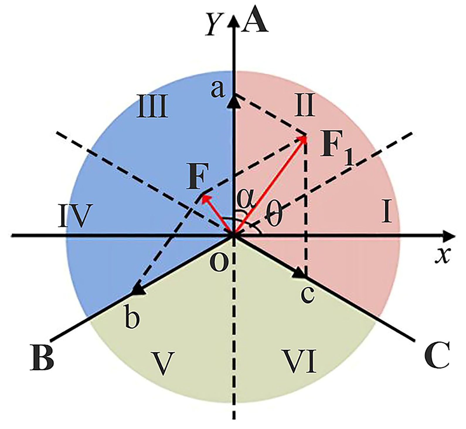
The essence of sustainable territorial spatial development lies in achieving coordination among production, living, and ecological functions. Drawing on the mechanical equilibrium model from physics and referencing relevant studies, this study objectively characterizes the dynamic trade-off process of LUFs. Figure 3 exhibits a pie chart for each county’s PF (a), LF (b) and EF (c) using the method described in Section 3.1. These abstractions show three component forces with equal angular intervals (2π/3) in different directions. The polar radius F represents the deviation index between the resultant force and equilibrium point O, where greater deviation indicates poorer LUF coordination.

The polar angle θ denotes the deflection angle in the equilibrium system, reflecting specific characteristics of LUF coordination. By extending OA, OB and OC in opposite directions, we divide the LUF into six quadrants. This delineation clarifies the vector characteristics of each quadrant and enables further identification of evolutionary features of dominant functions, as detailed in

Table 4. The characteristics of different coordination degree types of “production-living-ecological” function.

Quadrant	Angel Range	Force Characteristics
		Production Function	Living Function	Ecological Function
I	[11π/6,0], [0,π/6]	+	±	−
II	[π/6, π/2]	±	+	−
III	[π/2, 5π/6]	−	+	±
IV	[5π/6, 7π/6]	−	±	+
V	[7π/6, 3π/2]	±	−	+
VI	[3π/2, 11π/6]	+	−	±

Note: The signs +, − and ± indicate that the direction of the force is positive, negative, and uncertain, respectively.

.

$$\overrightarrow{OA}=(x_A,y_A)=(0,a)$$

(3)

$$\overrightarrow{OB}=(x_B,y_B)=\left[\cos \left(1/2(1-\left|b\right|/b)\pi -5\pi /6\right)\left|b\right|,\sin \left(1/2(1-\left|b\right|/b)\pi -5\pi /6\right)\left|b\right|\right]$$

(4)

$$\overrightarrow{OC}=(x_C,y_C)=\left[\cos \left(1/2(1-\left|c\right|/c)\pi -\pi /6\right)\left|c\right|,\sin \left(1/2(1-\left|c\right|/c)\pi -\pi /6\right)\left|c\right|\right]$$

(5)

$$\theta =\left\{\begin{array}{c}\arctan \left(y_F/x_F\right)+2\pi ,x_F\ge 0\\ \arctan \left(y_F/x_F\right)+\pi ,x_F<0\end{array}\right.$$

(6)

Establishing the objective function of the mechanical equilibrium model–NSGA-II coupling model based on Equations (1)–(6) sought to coordinate the development of production, living, and ecological functions of land use:

$$\begin{array}{l}F=\overrightarrow{OA}+\overrightarrow{OB}+\overrightarrow{OC}=(x_F,y_F)\\ =(x_A+x_B+x_C,y_A+y_B+y_C)\\ =(x_F,y_F)\\ =\min (f_1(X),f_2(X))\end{array}$$

(7)

a, b, and c represent the level values of the PF, LF, and EF of each county, respectively. $\overrightarrow{OA}$, $\overrightarrow{OB}$, and $\overrightarrow{OC}$ symbolize the forces of PF, LF, and EF, respectively; F represents the resultant force. x_A, x_B, x_C and x_F represent the component forces of $\overrightarrow{OA}$, $\overrightarrow{OB}$, $\overrightarrow{OC}$ and F along the X-axis direction, respectively. y_A, y_B, y_C and y_F represent the component forces of $\overrightarrow{OA}$, $\overrightarrow{OB}$, $\overrightarrow{OC}$ and F along the Y-axis direction, respectively. θ denotes the angle between the resultant force and the positive direction of the x-axis. f₁(X) minimizes the x-component of the resultant force, and f₂(X) minimizes the y-component.

The rationale is as follows: the mechanical equilibrium model developed in this study represents the trade-offs and synergies among production, living, and ecological functions as “opposing and cooperative forces” in a mechanical system, drawing on spatial equilibrium theory and the principle of vector addition. The ideal equilibrium point O of the mechanical equilibrium model is the zero vector; that is, the resultant-force vector F = (x_F, y_F) must approach (0, 0), with both components approaching zero simultaneously. Therefore, formulating the two axial components as two parallel and independent minimization objectives drives the system to converge toward the origin more precisely and allows individuals that are severely imbalanced along a single axis to be eliminated more rapidly during population evolution. This reflects the full meaning of the mechanical equilibrium model: equilibrium is not merely a matter of a small magnitude; it also requires directional balance. The two objectives therefore guide the system toward more accurate and robust convergence.

In addition, a resultant force of zero does not imply absolute equality of the three functions across counties; rather, it represents an idealized state of coordinated sustainable development. To reflect differences in main functional zoning and resource endowments between Zhejiang’s mountainous and coastal areas, we introduce differentiated weights that capture variations in functional priorities under the equilibrium objective. Drawing on policy documents such as the Zhejiang Provincial Main Functional Zoning Plan, the Zhejiang Provincial Territorial Spatial Master Plan (2021–2035), and the Implementation Plan for the High-Quality Leapfrog Development of 26 Mountainous Counties in Zhejiang Province (2021–2025), we classify the 33 counties into four types: ecology-priority, industry-dominated, liveable urban, and balanced coordinated development. Each type is assigned a distinct weight combination for production, living, and ecological functions (e.g., weights of 0.25, 0.25, and 0.50 for the ecology-priority type). To test the sensitivity of these weight settings to optimization outcomes, we design three gradient schemes (weak, medium, and strong) for each type (e.g., ecological weights of 0.4, 0.5, and 0.6 for the ecology-priority type). Through multi-scenario comparisons, we assess the discriminatory effects of the weighted priorities and model robustness, ensuring that the land use optimization plan for each county type aligns with its statutory development orientation.

2. Fixed Effects Model for CU and the LUFs

To examine the associations between land use functions (LUFs) and urbanization indicators, this study employs a fixed-effects panel regression design, based on 231 observations from 33 counties observed at seven time points each. By incorporating a fixed effect for year (year FE) to isolate county-specific characteristics from interference with the dependent variable, the model mitigates autocorrelation across time dimensions. A linear regression framework was adopted to enhance the generalizability of findings. We constructed three fixed-effects panel regression models (

Table 5. Panel fixed-effects regression table.

	a (PF)	b (LF)	c (EF)
x1	−0.12 ***	0.96 ***	−0.19 **
	(0.027)	(0.189)	(0.086)
x2	−0.09 ***	0.28 ***	0.09 **
	(0.011)	(0.080)	(0.037)
x3	0.01 *	0.19 *	−0.14 ***
	(0.012)	(0.102)	(0.045)
x4	0.10 ***	−0.34 ***	0.28 ***
	(0.021)	(0.107)	(0.069)
_cons	0.09 ***	0.01 *	0.11 ***
	(0.002)	(0.008)	(0.005)
Year FE	Yes	Yes	Yes
N	231	231	231

Standard errors in parentheses. * p < 0.10, ** p < 0.05, *** p < 0.01.

), where a, b, and c denote the respective levels of PF, LF, and EF. x1–x4 represent the levels of population urbanization, economic urbanization, social urbanization, and ecological urbanization, respectively.

As shown in Table 5, the regression coefficients of x1–x4 all pass statistical significance tests at varying levels (p < 0.10, p < 0.05, p < 0.01), indicating that improvements across multiple dimensions of urbanization are robustly associated with variations in different land use functions. To further assess the stability of these findings, two robustness checks—time segmentation (A) and winsorization (B)—were conducted (

Table 6. Robustness tests.

	a-A	a-B	b-A	b-B	c-A	c-B
x1	−0.19 ***	−0.12 ***	1.20 ***	1.10 ***	−0.01 **	−0.28 ***
	(0.051)	(0.027)	(0.279)	(0.179)	(0.088)	(0.088)
x2	−0.06 **	−0.09 ***	0.40 *	0.32 ***	0.04	0.10 **
	(0.029)	(0.011)	(0.217)	(0.082)	(0.052)	(0.039)
x3	−0.08 *	0.01	0.75 ***	0.21 **	−0.08 *	−0.16 ***
	(0.042)	(0.012)	(0.263)	(0.102)	(0.072)	(0.047)
x4	0.11 ***	0.10 ***	−0.08 *	−0.34 ***	0.18 ***	0.28 ***
	(0.036)	(0.021)	(0.233)	(0.108)	(0.063)	(0.072)
_cons	0.10 ***	0.09 ***	−0.02	0.01	0.11 ***	0.11 ***
	(0.008)	(0.008)	(0.016)	(0.012)	(0.011)	(0.010)
Year FE	Yes	Yes	Yes	Yes	Yes	Yes
N	132	231	132	231	132	231

Standard errors in parentheses. * p < 0.10, ** p < 0.05, *** p < 0.01.

). Both tests yield results consistent with the baseline estimates, supporting the conclusion that the fixed-effects panel framework provides credible and broadly generalizable evidence on the relationship between land use functions and urbanization indicators.

3.2.2. Model Variable Specification

First, this study constructed a land use quantity structure optimization model that integrates a mechanical equilibrium model and a multi-objective genetic algorithm (NSGA-II) based on the “land category-function” correspondence. The variables were various land use types m₁–m₆, corresponding to six categories: cropland (paddy fields and dryland), woodland (forest land, shrubland, open forest land, and other woodland), grassland (high-coverage, medium-coverage, and low-coverage grassland), water bodies (rivers/canals, lakes, reservoirs/ponds, beaches, and tidal flats), built-up land (urban land, rural residential areas, and other construction land), and unused land (bare soil and bare rock).

Second, the “urbanization driving force–PLE space evolution” framework helped establish the mapping relationships between urbanization dynamic mechanisms and PLE spatial functional demands using a mechanical model and optimize the urbanization subsystem structure. The model variables comprise county-level urbanization development subsystems: x_1,i–x_4,i represent the levels of population urbanisation (U_P), economic urbanisation (U_E), social urbanisation (U_S), and ecological urbanisation (U_C), respectively.

3.2.3. Constrained Conditions

1. Subsystems of Urbanization Development

Drawing on the relative standard determination method from sustainability assessment, the polar angle θ in 2020 was calculated for each county. Equation (6) helps determine its quadrant position and identify specific land use function characteristics. This established the following value ranges for each variable:

$$\begin{array}{l}\Delta x_{1,i}=\left\{\begin{array}{c}(\overline{x_1},1),\theta \in (\mathrm{II},\mathrm{III},\mathrm{IV},\mathrm{V})\\ (\overline{x_1},x_{1,i}),\theta \in (\mathrm{I},\mathrm{VI})\&x_1>\overline{x_{1,i}}\\ (0,\overline{x_1}),\theta \in (\mathrm{I},\mathrm{VI})\&x_{1,i}\le \overline{x_1}\end{array}\right., \Delta x_{2,i}=\left\{\begin{array}{c}(\overline{x_2},1),\theta \in (\mathrm{II},\mathrm{III},\mathrm{IV},\mathrm{V})\\ (\overline{x_2},x_{2,i}),\theta \in (\mathrm{I},\mathrm{VI})\&x_{2,i}>\overline{x_2}\\ (0,\overline{x_2}),\theta \in (\mathrm{I},\mathrm{VI})\&x_{2,i}\le \overline{x_2}\end{array}\right.,\\ \Delta x_{3,i}=\left\{\begin{array}{c}(\overline{x_3},1),\theta \in (\mathrm{I},\mathrm{IV},\mathrm{V},\mathrm{VI})\\ (\overline{x_3},x_{3,i}),\theta \in (\mathrm{II},\mathrm{III})\&x_{3,i}>\overline{x_3}\\ (0,\overline{x_3}),\theta \in (\mathrm{II},\mathrm{III})\&x_{3,i}\le \overline{x_3}\end{array}\right., \Delta x_{4,i}=\left\{\begin{array}{c}(\overline{x_4},1),\theta \in (\mathrm{I},\mathrm{II},\mathrm{III},\mathrm{VI})\\ (\overline{x_4},x_{4,i}),\theta \in (\mathrm{IV},\mathrm{V})\&x_{4,i}>\overline{x_4}\\ (0,\overline{x_4}),\theta \in (\mathrm{IV},\mathrm{V})\&x_{4,i}\le \overline{x_4}\end{array}\right.,\end{array}$$

(8)

and,

$$x_{1,i}+x_{2,i}+x_{3,i}+x_{4,i}\le 1$$

(9)

$\overline{x_1}$, $\overline{x_2}$, $\overline{x_3}$, and $\overline{x_4}$ represent the 2020 average levels of U_P, U_E, U_S, and U_C, respectively, in Zhejiang Province. x_1,i, x_2,i, x_3,i, and x_4,i denote the actual 2020 levels of U_P, U_E, U_S, and U_C, respectively, for the ith county unit.

2. Land Use Types

First, a multi-gradient sensitivity analysis with thresholds of ±10%, ±20%, and ±30% was performed on land use transformation constraints. The results verified that the optimized land use results in this study are highly robust. As documented by Wang et al. [27], land allocation schemes that drastically deviate from existing land use patterns can greatly raise land conversion costs and impede regional sustainable development. In contrast, excessively strict constraints would narrow the optimization space of land use structure and fail to achieve multi-objective coordinated equilibrium. Therefore, this study selected 20% as the unified overall threshold for land use conversion. Furthermore, in accordance with the regulatory requirements of the three control lines in Zhejiang Province—ecological protection redlines, permanent basic farmland, and urban development boundaries—differentiated constraint rules were established at the county level to refine the model’s constraint framework.

(1)

Total land area

This study sets the constraint of “total land area remains unchanged” for each county. First, this is based on empirical data from the study period (2000–2020) for the 33 counties in Zhejiang Province; remote sensing data shows that the total area of each county remained highly stable during the study period. Furthermore, the “Zhejiang Province Territorial Spatial Plan (2021–2035)” establishes “total quantity control” as a core management principle. Adjustments to land use at the county level must be carried out within the total quantity framework determined by the higher-level plan and cannot be exceeded without authorization. Finally, this study adopts the “total land area remains unchanged” constraint commonly used in previous sustainable land use optimization research [57,58].

(2)

Cultivated Land

Safeguarding national and regional food security constitutes the fundamental premise of cultivated land protection. Grain output from cultivated land (m₁), together with imports, should be equal to or greater than the food demand required to sustain the local population. This relationship can be expressed as

$$m_1{f}_2{f}_3{f}_4\ge P{f}_0{f}_1$$

(10)

where, P is the projected total population; f₀ is the per capita food demand, projected to reach 517.30 kg/person by 2030 [59]; f₁ is the food self-sufficiency rate; f₂ is the grain yield per unit area; f₃ is the ratio of grain crop sowing area to total crop sowing area; and f₄ is the multiple cropping index. The projections are generated using the GM (1,1) gray forecasting model, based on historical trajectories of socio-economic development and land use change in each county, and represent a baseline scenario without policy intervention [60].

(3)

Construction Land

The planned construction land quota for each county should be set such that, by the target year, the total amount of construction land (m₅) satisfies the following condition:

$$m_5/A\le Q$$

(11)

A is the total land area of the county, and Q is the planned land development intensity for the target year. Where a county has not specified an explicit cap on land development intensity, the amount of construction land should not exceed the gray-model forecast derived from historical trends under a non-intervention scenario.

(4)

Forest Cover Constraint

The lower bound of forest coverage is defined using the concept of the ecological green equivalent. Within the land system, land use types that contribute to the green equivalent include cultivated land, forest land, and grassland, with coefficients of 0.46, 1.00, and 0.49, respectively. Based on the forest cover targets stipulated in each county’s ecological construction plan for the target year, the constraint can be formulated as

$$0.46m_1+m_2+0.49m_3\ge At$$

(12)

m₁, m₂, and m₃ represent the areas of cultivated land, forest land, and grassland, respectively; A is the total land area of each county; and t is the planned forest coverage rate.

3.2.4. The Pareto Optimization Strategy

The optimal decision followed after the Pareto solution set of the land use structure optimization model by identifying the solution with the maximum combined value of PF (a), LF (b) and EF (c) functions. Similarly, the Pareto frontier helped select the urbanization subsystem structure optimization model, the optimal solution based on two criteria: (1) satisfying the threshold requirements for PF, LF, and EF (a, b, and c) and (2) maximizing the sum of these functional values.

3.2.5. Model Validation

The parameter settings for the NSGA-II algorithm used in this study are detailed in Appendix B. The model simulation results were validated using a retrospective optimization approach. The validation outcomes show that across all 33 county-level units, the mean coefficient of determination (R²) reached 0.784 (range: 0.646–0.896), and the mean absolute percentage error (MAPE) averaged 11.61% (range: 5.91–15.39%), indicating relatively robust results.

Compared with standard genetic algorithms (GAs), particle swarm optimization (PSO), and multi-objective particle swarm optimization (MOPSO), NSGA-II proved considerably more adaptable to the problem in this study. For one thing, both GA and classical PSO were originally designed for single-objective problems—even when repurposed for multi-objective tasks through weighting or other scalarization tricks, they struggle to capture the underlying trade-offs and synergies among objectives. MOPSO, on the other hand, does support multi-objective optimization, but its velocity-position update mechanism, built for continuous spaces, tends to lose efficiency and global search capability when applied to discrete land use structure variables. Taken together, this makes NSGA-II a more suitable and defensible solution framework for the multi-objective land use optimization pursued here.

4. Results

4.1. Evolution Characteristics of Urbanization Subsystem

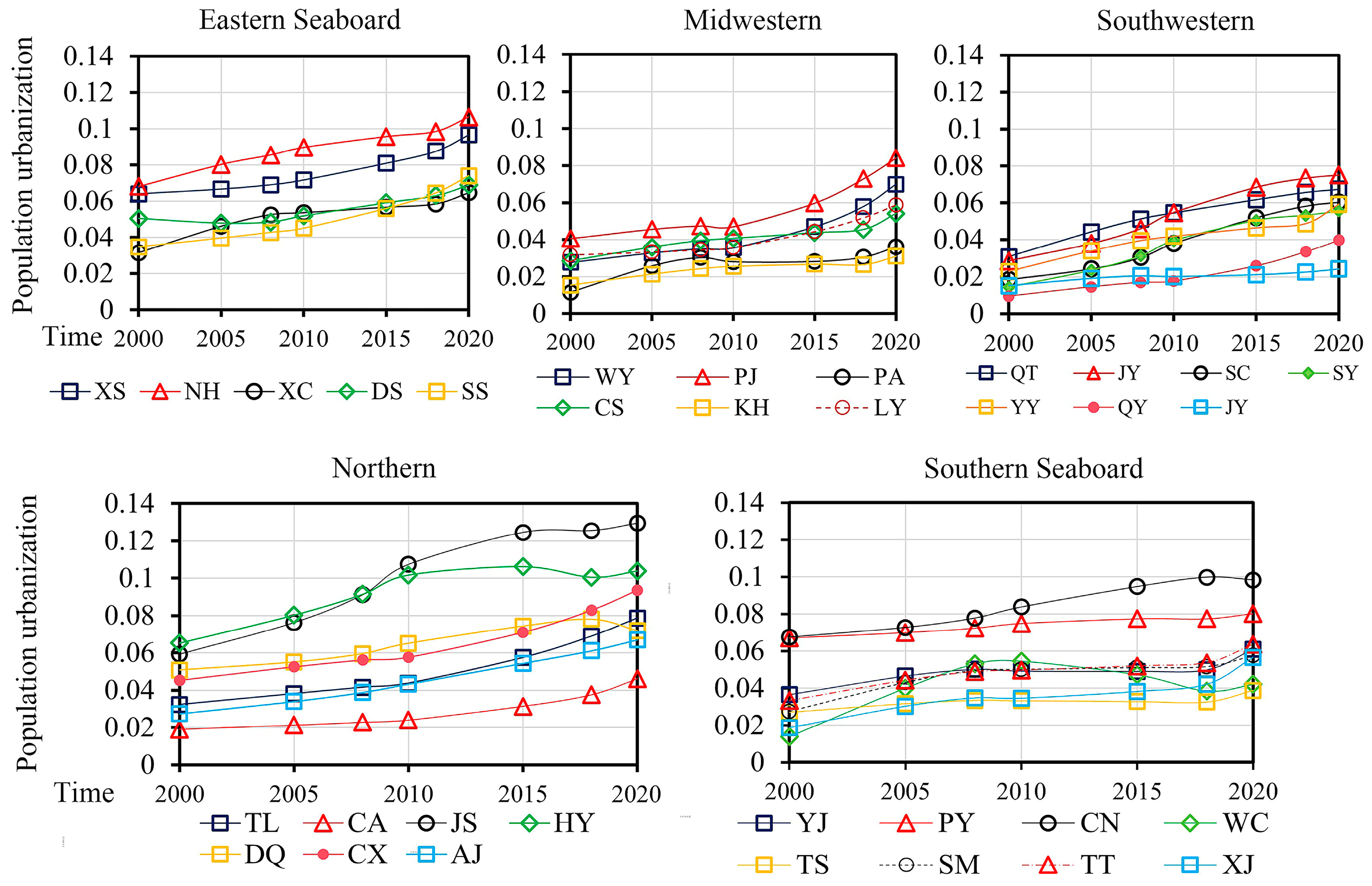
Based on the established evaluation framework, this study systematically assessed the urbanization subsystem development across all counties in Zhejiang Province from 2000 to 2020. As shown in Figure 4, although the province exhibited an overall upward trend in population urbanization rate, significant regional disparities were observed: counties in the central-western and southwestern regions maintained relatively low urbanization levels (0.01–0.08), with the southwest showing steady growth while central-western counties such as PJ and WY accelerated after 2015; the southern coastal area (excluding CN) progressed more slowly and remained below 0.1 throughout the period. In contrast, eastern coastal and northern counties experienced more pronounced development: eastern counties like NH and XS already reached 0.06 at the start of the study, and northern counties including JS and HY exceeded 0.1 after 2015. The results reveal a distinct tiered spatial pattern of population urbanization in Zhejiang Province: “northeast leading–southern coast intermediate–central-western and southwestern regions lagging”, with consistently widening regional disparities.

This pattern has emerged through the combined influence of multiple factors. Among them, location and the spillover effects of central cities are the underlying drivers of the east–west divide. Northeastern counties lie close to core cities such as Hangzhou and Ningbo and are strongly influenced by their industrial spillovers and population agglomeration effects. In contrast, most southwestern counties are mountainous, have poor transport accessibility, and find it difficult to effectively absorb functions decentralized from central cities. In addition, manufacturing and modern services dominate the eastern coastal and northern plain areas, creating large numbers of non-agricultural jobs and continually attracting inward migration. By contrast, the mountainous counties of the southwest rely mainly on agriculture and forestry; their limited capacity to accommodate non-agricultural employment makes it difficult to generate sustained momentum for population concentration.

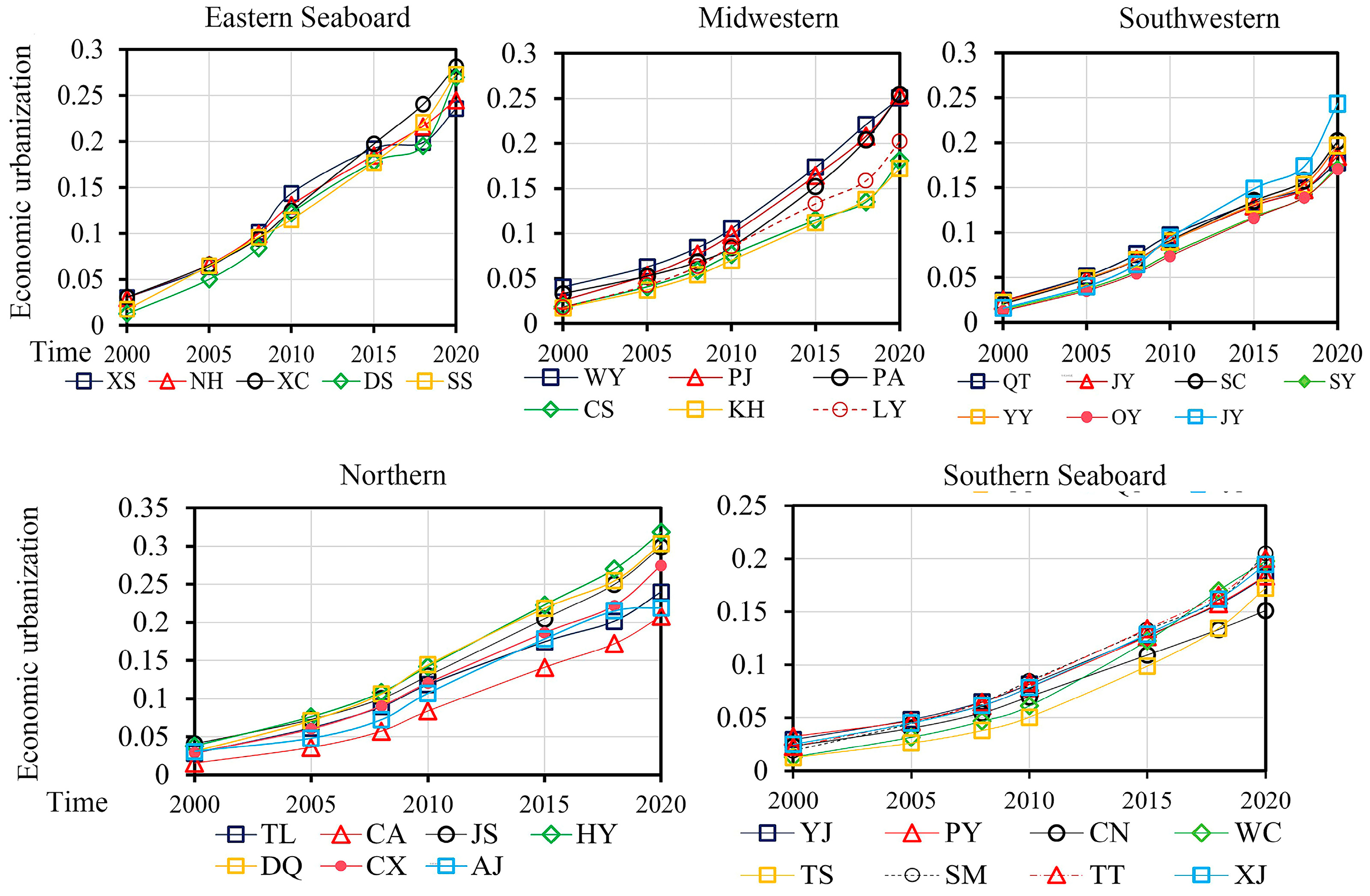
Figure 5 reveals consistent growth in all regions from 2000 to 2020, with high homogeneity within each region. At the outset of the study period, regions displayed generally low economic urbanization levels (0–0.05) and minimal inter-regional disparity. After 2010, gaps began to emerge: by 2015, eastern coastal and northern regions reached 0.15–0.2, whereas southern coastal and southwestern inland areas remained at 0.1–0.15. Differentiation intensified after 2015—eastern coastal counties collectively exceeded 0.2, and most northern along with selected central counties also surpassed 0.2, while most southwestern and southern coastal counties stayed below that threshold. This spatial pattern highlights a clear regional divide in Zhejiang’s economic urbanization, characterized by “leading eastern coastal and northern regions versus relatively lagging southwestern and southern coastal areas”.

From the perspective of driving mechanisms, the northern and eastern coastal areas have developed highly competitive industrial clusters, with well-developed industrial chains and pronounced agglomeration effects, sustaining growth in regional economic output. By contrast, counties in the southwest are dominated by resource-based industries and agricultural processing. Their industrial chains are short, value added is low, and the momentum for economic growth is weak. Differences in local fiscal capacity and investment levels must also be considered. Regions that developed earlier can draw on strong fiscal foundations to continuously increase investment in industrial platforms and infrastructure, creating a virtuous cycle of “growth–investment–further growth”, whereas lagging regions have made little progress in economic urbanization.

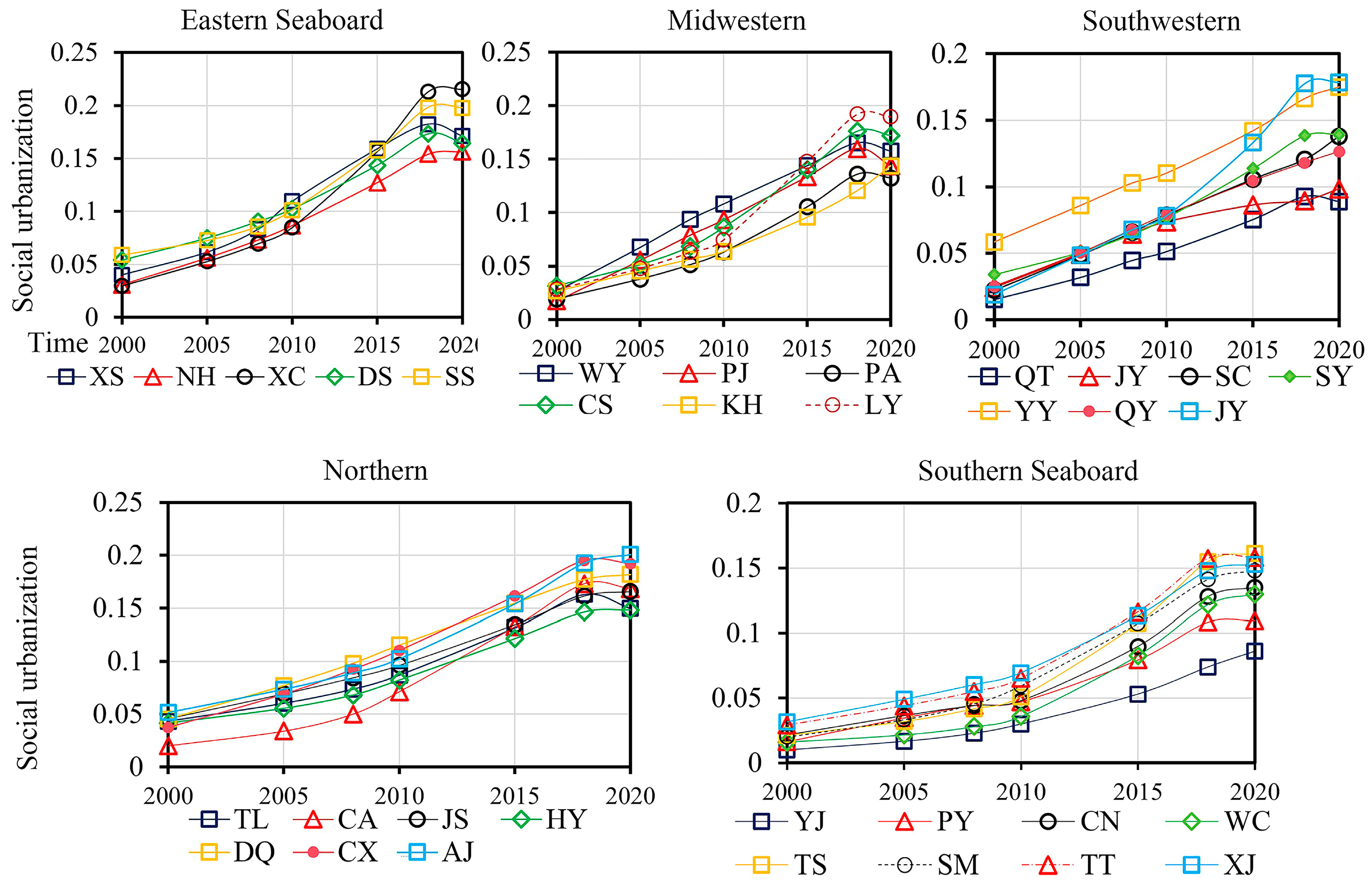
As depicted in Figure 6, the social urbanization level in Zhejiang Province followed a pattern of “initial growth followed by stabilization”: it rose continuously from 2000 to 2018 and then plateaued between 2018 and 2020. Regionally, counties in the eastern coastal, northern, and central-western areas showed strong developmental consistency, whereas distinct disparities persisted in the southern coastal and southwestern regions. Notably, since 2015, most eastern coastal and northern counties have exceeded the threshold of 0.15 in social urbanization. This trajectory reflects a clear spatial differentiation in county-level social urbanization across Zhejiang, characterized by “higher levels in the northeast and lower levels in the southwest.”

The evolution of this pattern can be explained from both the demand and supply sides. On the demand side, the scale and composition of population concentration determine the spatial distribution of demand for public services. Northeastern counties have high population densities and large concentrations of migrant workers, generating strong demand for education, healthcare, social security, and other public services and thereby raising the level of social urbanization. In contrast, southwestern counties have relatively small populations and continue to experience out-migration; demand is therefore too limited to generate economies of scale in public service provision. On the supply side, disparities in local fiscal revenue directly determine the capacity to provide public services.

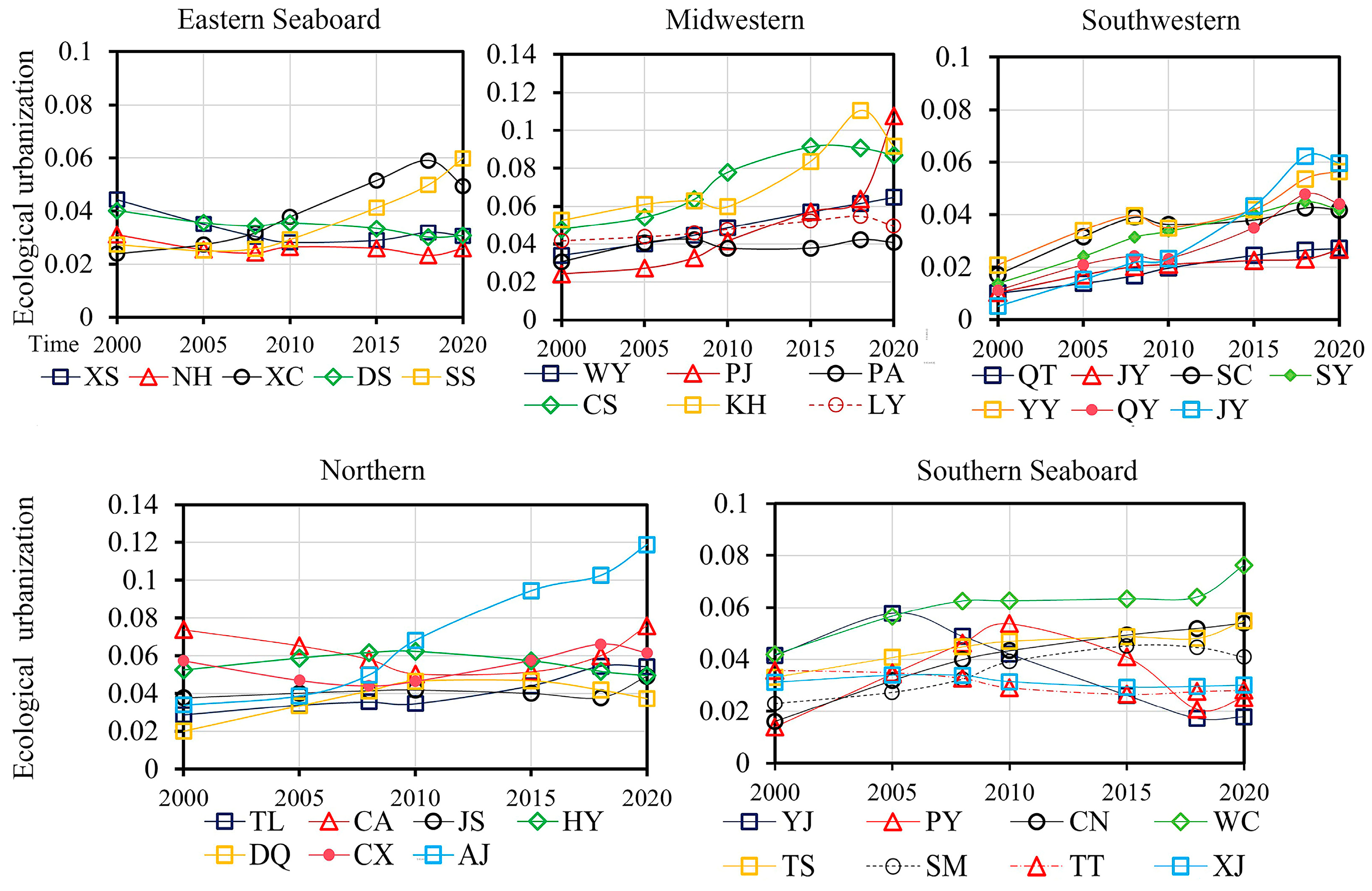
This study systematically evaluated the development of ecological urbanization across counties in Zhejiang Province (Figure 7). The results show significant spatial differentiation in developmental trajectories: the northern region displayed divergent pathways, with AJ County growing rapidly to 0.14 after 2010 while other northern counties remained relatively stable. Selected counties in the central-western (KH, CS) and southwestern (JN, YH) regions also maintained sustained upward trends. In terms of development levels, a clear spatial gradient emerged after 2010. Most counties in the eastern coastal, southern coastal, and southwestern regions remained within the 0.01–0.06 range, whereas certain northern and central-western counties progressed into the 0.06–0.12 range. Overall, inter-county disparities in ecological urbanization showed a persistent widening trend.

The driving mechanisms of ecological urbanization are distinctive and should be understood in terms of three dimensions: natural baseline conditions, stage of development, and policy response. In terms of natural baseline conditions, counties differ inherently in their ecological resource endowments, providing the objective basis for divergent development trajectories. In terms of development stage, regions that industrialized earlier face mounting ecological and environmental pressures in the middle and later stages of industrialization. Coupled with rising public expectations for environmental quality, these pressures compel local governments to increase investment in ecological conservation and environmental governance, thereby accelerating ecological urbanization. In terms of policy response, some counties have drawn on provincial earmarked funding to substantially increase investment in ecological governance, effectively sustaining improvements in ecological urbanization.

4.2. Evolution Characteristics of LUFs

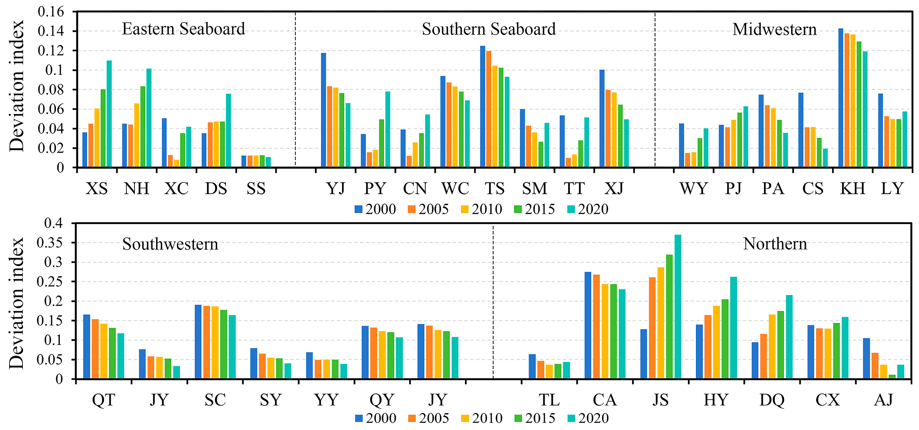
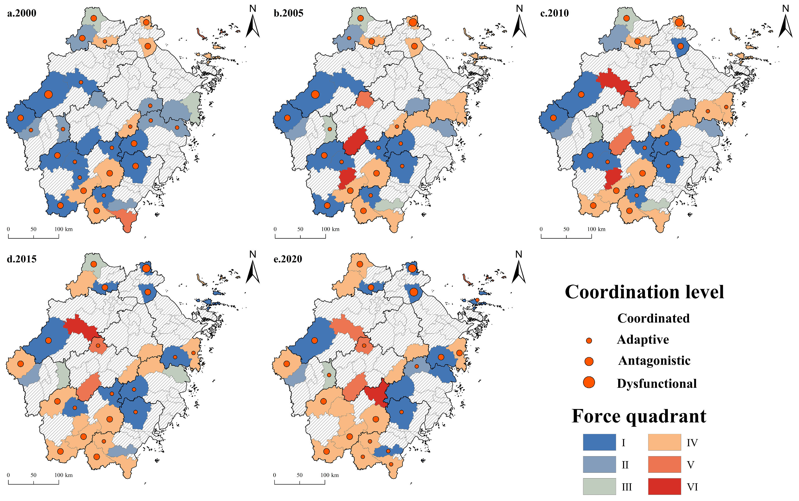
Based on the LUF evaluation system and mechanical equilibrium model, this study analyzed land use changes across Zhejiang counties from two dimensions: the functional deviation index (Figure 8) and dominant functional characteristics (Figure 9). A lower functional deviation index indicates stronger synergy among production, living, and ecological functions. Clarifying their coordination and the evolution of dominant functions is key to guiding land use transition, optimizing spatial structure, and improving territorial sustainability. As shown in Figure 8, the PLE functional deviation index displayed pronounced spatial heterogeneity (ranging from 0.01 to 0.4) and distinct evolutionary patterns during 2000–2020. The northern region underwent the most marked fluctuations (0.01–0.37), whereas the southwestern region remained relatively stable (0.04–0.2). The eastern coastal, southern coastal, and central-western regions, despite notable internal variation, largely fell within the 0.02–0.14 interval. Overall, a three-tier gradient pattern emerged: “northern region > southwestern region > southeastern coastal and central-western regions”. These spatial disparities reflect the combined effects of rapid urbanization in the north, stronger ecological protection in the southwest, and moderate transitional dynamics in the coastal and central-west areas.

As shown in Figure 9, this study categorized counties in Zhejiang into four types: “coordinated” (0–0.05), “adaptive” (0.05–0.1), “antagonistic” (0.1–0.25), and “dysfunctional” (0.25–0.4). During 2000–2020, two dominant patterns emerged: high-production–low-ecology (type I) and high-ecology–low-production (type IV). Type I was mainly concentrated in the northern, central-western, and eastern coastal regions, while type IV prevailed in the southwestern and southern coastal areas. Most counties remained in the “coordinated” or “adaptive” categories; these areas require enhanced monitoring of their weaker functions to prevent disparities from widening. In contrast, “antagonistic” and “dysfunctional” regions call for differentiated regulatory measures. By 2020, JS and HY in the north fell into the high-production–low-ecology “dysfunctional” zone, whereas CA (northern) and NH (eastern coastal) belonged to the high-production–low-ecology “antagonistic” category—both characterized by elevated production but depressed ecological functions. Regulatory strategies here should focus on optimizing urban land use structures, preventing illegal conversion of ecological land to construction uses, and expanding green infrastructure. Conversely, the high-ecology–low-production “antagonistic” zone included SC, QT, JN, and QY in the southwest, as well as KH in the central-west, where ecological functions outweighed production. Such regions could develop specialty industries that enhance production without compromising ecological integrity.

5. Discussion

5.1. Optimization Analysis and Regulation Strategies for Urbanization Subsystems

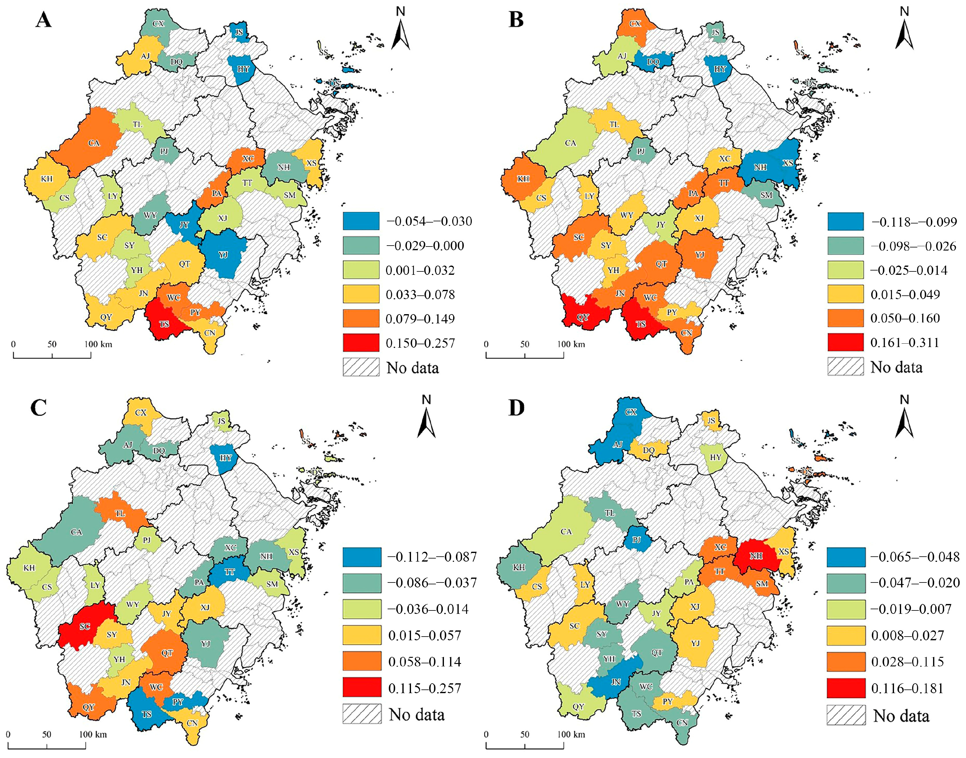
Figure 10 shows the structural optimization requirements of the urbanization subsystems in 33 counties of Zhejiang Province. It should be noted that this study optimizes the land use structure with the coordination of PLE spatial functions as its objective. In addition, fixed-effects panel regression is used to establish a quantitative mapping between urbanization indicators and the evolution of PLE functions, thereby enabling coordinated regulation of the population, economic, social, and ecological subsystems. The optimization requirements of the individual subsystems therefore represent the relative direction and magnitude of adjustment under the established objective of coordinated PLE development. The following analysis seeks to identify patterns of deviation between the current values of each subsystem and its optimization targets, providing a reference for differentiated regulation.

With respect to population urbanization (Figure 10A), the optimization requirements exhibit a discernible regional gradient. In some southern coastal and southwestern counties, such as TS and YH, current values differ substantially from the optimization targets and need to increase by 0.08–0.26. Some central (PA), eastern (XC), and northern (CA) counties require moderate increases of 0.08–0.15, whereas several developed counties in the north and along the eastern coast require slight downward adjustments of 0–0.03. To some extent, this distribution of deviations reflects regional differences in the degree to which population urbanization levels align with the objective of coordinating spatial functions. However, these differences should not be read directly as a ranking of the degree of “development imbalance,” because the optimization requirements for population urbanization are also influenced by each region’s role in the province-wide division of spatial functions. For example, a slight downward adjustment in developed areas may reflect saturation of the spatial carrying capacity of urban core areas rather than insufficient development.

Figure 10B shows the optimization deviations in the economic urbanization subsystem. Some counties in northern Zhejiang and along the southern coast, such as XS and NH, require moderate downward adjustments in their economic urbanization indicators (0–0.12), whereas most southwestern counties, except JN and JY, require substantial increases (0.1–0.31). The deviations for TS and QY are especially pronounced, with a maximum required increase of 0.3. It should be emphasized that these results represent indicator deviations under the objective of coordinating spatial functions. Because this study does not impose quantitative constraints on economic feasibility factors, such as the infrastructure investment associated with improvements in economic urbanization, the substantial increases required in the southwest must be assessed cautiously during policy formulation, taking local fiscal capacity into account.

As shown in Figure 10C, current social urbanization values in the southwest, except YH, differ substantially from the optimization targets and need to increase by 0.015–0.26, indicating considerable scope for improvement in public services and social security systems. Some northern (TL and CX), eastern coastal (SS), and central-western (XJ) counties require moderate increases of 0–0.12. Counties whose current values have reached or exceeded their optimization targets may face the risk of an excessive concentration of public-service resources or declining marginal efficiency in resource allocation. They should therefore be assessed on the basis of local conditions rather than simply regarded as requiring a “mandatory reduction”.

Figure 10D shows the optimization deviations in the ecological urbanization subsystem. Counties in the southwest generally require moderate downward adjustments of 0.02–0.05, whereas southeastern coastal counties, particularly NH, should be prioritized for increases of 0.12–0.19. The distribution of deviations is shaped by the combined effects of each county’s natural endowments, its existing ecological land base, and other factors. Overall, this analysis of optimization deviations provides a reference for the direction of adjustment from the perspective of coordinated PLE development. In practice, however, the regulatory directions identified in this study should be adjusted in light of local fiscal capacity, policy feasibility, and other factors.

5.2. Optimization Analysis and Regulation Strategies of Land Use Structure in County-Level Regions

5.2.1. Optimal Quantification of Diverse Land Use Types

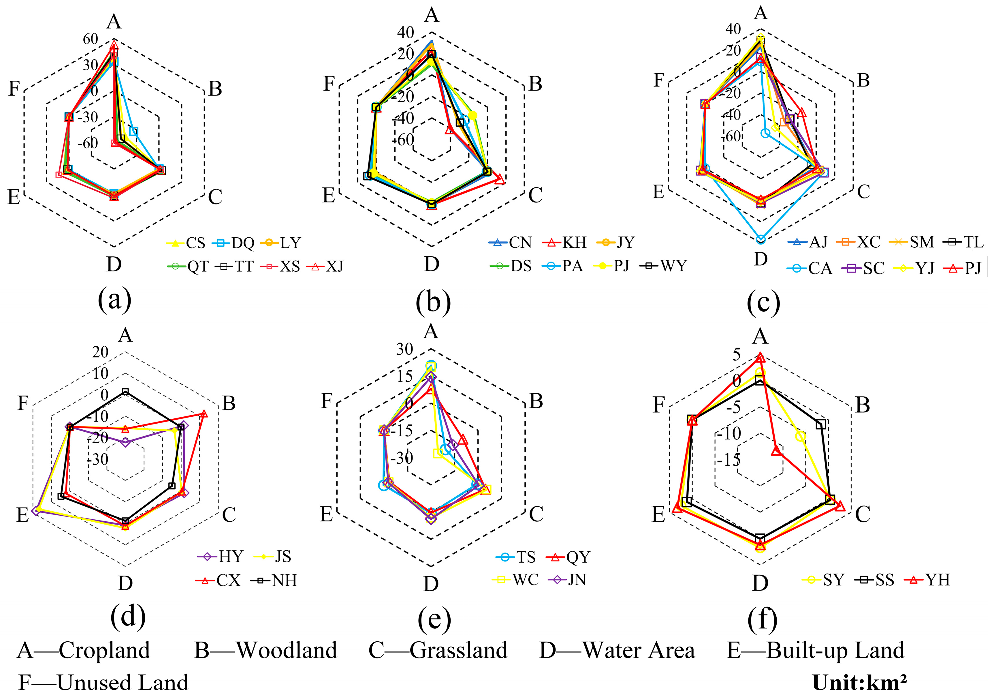
As illustrated in Figure 11, the optimized land use area of individual counties differs substantially from the baseline conditions in 2020, revealing distinct spatial heterogeneity in regional land use structures.

The counties shown in Figure 11a–c follow a composite trajectory of “substantial cropland expansion–marked forestland contraction, slight increases in water bodies and grassland–moderate growth in construction land”. This corresponds to a PLE restructuring pattern characterized by strong expansion of production space, moderate expansion of living space, and severe contraction in the total area of ecological space, accompanied by minor internal structural adjustments. The dominant conversion pathway is from forestland to cropland and construction land. The counties shown in Figure 11d exhibit an optimization pattern of “construction land expansion–marked cropland reduction–minor forestland fluctuation”, corresponding to a PLE restructuring pattern in which living space expands, production space contracts, and ecological space remains stable.

Figure 11e exhibits a pattern of synergistic ecological optimization characterized by “steady cropland growth–forestland reduction, concurrent increases in grassland and water bodies–negative growth in construction land”. The corresponding PLE restructuring pattern involves moderate expansion of production space, improvement in the quality of ecological space, and contraction of living space through more intensive use. Although forestland is the principal land type being converted, the substantial increase in grassland (+2.5 km²) and marked increase in water bodies (+2.0 km²) indicate a positive structural substitution within ecological land. At the same time, construction land decreases by an average of approximately 2.2 km², with QY and WC among the counties recording negative values, while unused land remains largely stable. This pattern represents a relatively desirable reduction-oriented development pathway: reclaiming inefficient construction land and optimizing the allocation of ecological land improve ecological functions while maintaining food production. This pattern echoes the internationally advocated approach of “optimizing existing land stock”.

The counties shown in Figure 11f exhibit “the smallest changes across all land use categories”, corresponding to a “stable adjustment/low-carbon maintenance” optimization pattern. Their PLE restructuring is characterized by the basic preservation of the existing balance among production, living, and ecological spaces, with no major functional conversion.

The four PLE restructuring patterns identified in this study show both similarities to and differences from studies of land use change in other regions worldwide [61,62]. A common feature is that worldwide, the expansion of production and living spaces often comes at the cost of contraction in ecological space or production space (cropland). The difference is that a more diverse range of regulatory pathways is evident at the county level in China—particularly the “reduction in construction land + improvement in the quality of ecological space” pattern represented by Figure 11e and the “stable maintenance” pattern represented by Figure 11f—and these pathways have rarely been systematically reported in the international literature. This divergence may stem from China’s unique territorial spatial planning system and cropland protection policies. It provides a distinctive practical point of reference for land use regulation worldwide.

5.2.2. The Shares of Each Land Use Type in Total Land Area Before and After Optimization

Consistent with the optimization objectives of promoting coordinated development of PLE functions,

Table 7. Comparison of land use quantitative structure between the land use status in 2020 (A) and optimal plan (O) in 33 Counties of Zhejiang Province.

County		Cropland (%)		Woodland (%)		Grassland (%)		Water Area (%)		Built-Up Land (%)		Unused Land (%)
		A	O	A	O	A	O	A	O	A	O	A	O
Northern	AJ	23.42	24.66	67.84	66.26	2.77	2.71	1.35	1.45	4.60	4.90	0.02	0.02
	CA	6.91	7.13	78.46	77.21	3.35	3.53	10.38	11.22	0.88	0.89	0.02	0.02
	CX	48.65	47.54	39.95	40.81	0.62	0.64	2.55	2.63	8.16	8.31	0.07	0.07
	DQ	42.32	45.92	37.38	33.78	0.71	0.72	6.51	6.36	13.04	13.19	0.04	0.03
	JS	52.85	49.88	4.75	4.05	0.88	0.94	9.04	9.47	32.47	35.66	0.00	0.00
	HY	63.70	59.52	4.12	4.37	3.35	3.67	3.77	3.93	25.04	28.49	0.02	0.02
	TL	14.10	15.70	78.42	76.86	1.60	1.29	2.00	2.15	3.88	4.00	0.00	0.00
Eastern Coastal	XS	28.06	31.58	55.72	50.53	2.25	2.43	5.63	5.93	8.31	9.52	0.02	0.01
	NH	24.52	24.61	60.42	60.41	2.93	2.64	5.74	5.67	6.37	6.65	0.02	0.02
	XC	22.92	25.15	67.96	65.13	3.03	3.35	1.21	1.25	4.88	5.11	0.00	0.00
	DS	23.7	27.6	48.6	42.9	0.13	0.11	8.89	8.37	18.7	21.0	0.00	0.00
	SS	0.00	0.00	62.22	58.79	16.30	17.07	0.82	0.98	20.66	23.16	0.00	0.00
Southern Coastal	YJ	14.30	15.51	79.51	77.85	2.18	2.36	1.29	1.35	2.59	2.80	0.13	0.12
	PY	24.56	27.94	60.86	57.22	5.48	5.45	1.46	1.59	7.64	7.80	0.00	0.00
	CN	25.70	28.85	63.86	59.85	3.50	3.77	0.62	0.63	6.28	6.85	0.05	0.04
	WC	8.97	10.50	85.37	83.41	2.73	3.14	1.49	1.74	1.38	1.15	0.06	0.06
	TS	9.19	10.37	86.90	85.72	1.30	1.26	1.11	1.14	1.49	1.50	0.00	0.00
	SM	27.35	29.88	55.10	52.21	3.92	3.44	7.05	7.51	6.57	6.96	0.01	0.01
	TT	23.39	26.46	68.30	64.75	2.89	3.16	0.63	0.70	4.78	4.92	0.01	0.01
	XJ	16.55	19.20	79.00	76.09	1.48	1.56	0.58	0.64	2.40	2.51	0.00	0.00
Central-Western	WY	18.41	19.63	75.19	73.32	0.89	0.91	0.59	0.62	4.85	5.44	0.08	0.08
	PJ	19.80	21.18	71.61	69.91	1.59	1.66	0.79	0.72	6.18	6.50	0.03	0.03
	PA	12.49	14.05	81.52	79.45	2.83	2.82	0.05	0.06	3.10	3.63	0.00	0.00
	CS	23.44	26.87	64.48	60.32	7.13	7.30	1.51	1.70	3.43	3.80	0.02	0.02
	KH	12.02	13.05	82.42	80.63	4.32	4.92	0.20	0.24	1.03	1.14	0.02	0.02
	LY	34.01	37.94	54.53	50.12	2.90	2.91	2.48	2.38	6.01	6.60	0.06	0.05
Southwestern	QT	10.26	12.06	84.39	82.15	1.75	1.93	2.08	2.11	1.49	1.72	0.03	0.03
	JY	13.95	15.87	81.00	78.92	1.03	1.04	0.52	0.55	3.49	3.61	0.01	0.01
	SC	5.53	6.03	89.35	88.23	3.28	3.60	0.65	0.75	1.03	1.22	0.16	0.16
	SY	13.94	14.05	80.90	80.47	1.44	1.47	0.78	0.91	2.77	2.94	0.17	0.17
	YH	7.23	7.67	85.05	83.89	1.96	2.22	2.28	2.41	3.39	3.72	0.09	0.09
	QY	6.91	7.33	89.65	89.14	1.69	1.95	0.18	0.20	1.50	1.32	0.07	0.07
	JN	5.78	6.53	89.50	88.67	1.53	1.55	1.67	1.87	1.50	1.36	0.02	0.02

reports the shares of each land use type in total land area before and after optimization.

With respect to cropland, under the dual objectives of safeguarding food security and advancing coordinated PLE development, most counties in the study area need to increase the proportion of cropland, with an average increase of approximately +1.37% across all counties. The central-western region has a relatively high average increase of +2.09%, while the southwest has a smaller average increase of +0.85%. By contrast, the northern region records a slight average decrease (−0.23%), indicating marked regional differences.

Forestland shows an overall downward trend, with an average change of approximately −2.15% across all counties. The eastern coastal region records the largest reduction, averaging −3.43%, with particularly pronounced contractions in XS (−5.19%) and DS (−5.70%). The reductions are relatively smaller in the north and southwest, at −1.08% and −1.20%, respectively. Notably, the proportion of forestland increases slightly in some northern counties, such as CX and HY, reflecting differentiated adjustments to forestland.

Construction land generally needs to expand, with an average increase of +0.56% across all counties. The eastern coastal region requires the largest increase (+1.30% on average), followed by the north (+1.05%). Variation within the north is substantial, with large increases in counties such as JS (+3.19%) and HY (+3.45%). The southwest requires the smallest increase (+0.10%), while QY (−0.18%) and JN (−0.14%) in this region show downward trends.

The proportion of grassland changes only slightly, showing a marginal overall increase (approximately +0.11% on average) and no pronounced spatial heterogeneity. The area of water bodies also increases slightly, by approximately +0.10% on average across all counties, with larger required increases in the north (+0.23%) and along the southern coast (+0.13%). The proportion of unused land changes very little and has a negligible effect on the overall structure. The optimization results of this study differ from strategies in European and North American countries that emphasize ecological network protection: this study places greater emphasis on safeguarding food security as a baseline requirement, and the resulting increase in cropland is therefore greater than in comparable international cases. In addition, the internal differences identified in Zhejiang Province—including low growth in the southwest and a decline in cropland in the north—are consistent with international experience in differentiated management of mountainous and plain regions. However, this study quantifies specific adjustment thresholds at the county level and is therefore more fine-grained.

6. Conclusions

This study realizes the innovative integration of methodology by integrating the mechanistic equilibrium model that can depict the intrinsic interaction mechanism of the system (such as the trade-off relationships between functions) and the multi-objective optimization algorithm that can efficiently search the multi-dimensional solution space. This integration effectively overcomes the limitations of existing research, which mostly remains at isolated static evaluation or is limited to single-objective optimization (such as only pursuing the maximization of economic benefits), and quantitatively optimizes the quantity of land use types through the macro and principled “PLE coordination” concept via systematic mechanisms. It provides a reference method at the quantitative level of land use for solving the problem of “how to realize the coordinated optimization of the three PLE functions” in territorial and spatial planning. The key conclusions are summarized as follows.

6.1. Main Findings

Land use quantity structures display differentiated optimization pathways. For the majority of counties, the dominant transformation mode features expansion of cropland and construction land alongside the shrinkage of forestland. This corresponds to a spatial development mode where production and living spaces expand outward, accompanied by the reduction of ecological space capacity. In contrast, a subset of counties has achieved coordinated and sustainable development of production–living–ecological (PLE) spaces by revitalizing inefficient construction land. This is reflected in steady cropland growth, reduced forestland, simultaneous increases in grassland and water bodies, and negative growth in construction land—indicating positive structural substitution within ecological land. The optimization results for urbanization subsystems show that southern coastal and southwestern counties require targeted improvements in population and socioeconomic urbanization, northern counties call for differentiated ecological urbanization regulation, and southeastern coastal areas should prioritize ecological protection.

6.2. Scientific Contributions

This study innovatively combines a mechanical equilibrium model with the NSGA-II algorithm. Its core goal is to convert the macroscopic guiding principle of PLE functional coordination into quantifiable land use adjustment plans, which represents an improvement over previous studies relying only on static assessment or single-objective optimization. At the theoretical level, grounded in the recognition that urbanization is the core driver of land use function evolution and that land resources provide the material foundation for urban development, we construct a quantitative mapping between urbanization subsystems and PLE function dynamics, offering a more integrated analytical perspective for county-level research. In terms of empirical findings, the PLE restructuring pattern identified in this study—characterized by “reduction in construction land + improvement in the quality of ecological space”—improves ecological functions through reclaiming inefficient construction land and optimizing ecological land allocation, while maintaining food production. This pattern may offer useful reference for land use optimization at the county level.

6.3. Practical Implications

(1) Local governments and planning authorities could use this study for preliminary diagnosis. By applying the calculated functional deviation index and optimization deviations of urbanization subsystems, they could assess the gap between current conditions and targets for each county. This approach may serve as a pre-assessment tool for annual territorial spatial planning evaluations. (2) The results of changes in land use proportions could provide a quantitative benchmark for adjusting planning targets. Counties are advised to refer to the specific optimization outcomes when decomposing land use type targets in their master plans or annual implementation plans. (3) We recommend zone-based regulation according to the four identified PLE restructuring patterns. The framework could also be re-run every five years using the latest land use change survey data, allowing for dynamic updates of optimization targets.

6.4. Limitations and Future Research

While this work achieves robust optimization results and methodological advances for land use quantity structure and urbanization subsystems, it still has several limitations. First, data interpolation and grid aggregation may bring uncertainties to the results. Model parameters and constraints are calibrated based on county-level conditions in Zhejiang Province, so their transferability across other regions and computational scalability need further verification. Second, the optimized targets for urbanization only offer relative guidance under preset objectives. The research fails to quantify economic trade-offs such as financial affordability and does not evaluate cross-regional externalities caused by spillover effects.

Future work can incorporate cost–benefit analysis and spatial econometric models to quantify cross-border spillover impacts including ecological dividends and industrial radiation. This will help improve the holistic and systematic evaluation of land use optimization schemes.

References

1. Angel, S. Urban forms and future cities: A commentary. Urban Plan. 2017, 2, 1–5. [Google Scholar] [CrossRef] [Scilit]
2. Fan, Y.; Gan, L.; Hong, C.; Jessup, L.H.; Jin, X.; Pijanowski, B.C.; Sun, Y.; Lv, L. Spatial identification and determinants of trade-offs among multiple land use functions in Jiangsu Province, China. Sci. Total Environ. 2021, 772, 145022. [Google Scholar] [CrossRef] [Scilit] [PubMed]
3. Quintero-Gallego, M.E.; Quintero-Angel, M.; Vila-Ortega, J.J. Exploring land use/land cover change and drivers in Andean mountains in Colombia: A case in rural Quindío. Sci. Total Environ. 2018, 634, 1288–1299. [Google Scholar] [CrossRef] [Scilit] [PubMed]
4. Chen, Y.; Chen, Z.; Xu, G.; Tian, Z. Built-up land efficiency in urban China: Insights from the General Land Use Plan (2006–2020). Habitat Int. 2016, 51, 31–38. [Google Scholar] [CrossRef] [Scilit]
5. Zhuang, L.; Ye, C. Changing imbalance: Spatial production of national high-tech industrial development zones in China (1988–2018). Land Use Policy 2020, 94, 104512. [Google Scholar] [CrossRef] [Scilit]
6. Peters, D.J.; Hamideh, S.; Zarecor, K.E.; Ghandour, M. Using entrepreneurial social infrastructure to understand smart shrinkage in small towns. J. Rural Stud. 2018, 64, 39–49. [Google Scholar] [CrossRef] [Scilit]
7. Ding, C.; Zhao, X. Land market, land development and urban spatial structure in Beijing. Land Use Policy 2014, 40, 83–90. [Google Scholar] [CrossRef] [Scilit]
8. Zhang, Y.; Ding, X.; Dong, L.; Yu, S. Research on spatiotemporal patterns and influencing factors of county-level urban shrinkage in urbanizing China. Sustain. Cities Soc. 2024, 109, 105544. [Google Scholar] [CrossRef] [Scilit]
9. Steinhäußer, R.; Siebert, R.; Steinführer, A.; Hellmich, M. National and regional land-use conflicts in Germany from the perspective of stakeholders. Land Use Policy 2015, 49, 183–194. [Google Scholar] [CrossRef] [Scilit]
10. Paracchini, M.L.; Pacini, C.; Jones, M.L.M.; Pérez-Soba, M. An aggregation framework to link indicators associated with multifunctional land use to the stakeholder evaluation of policy options. Ecol. Indic. 2011, 11, 71–80. [Google Scholar] [CrossRef] [Scilit]
11. Aubry, C.; Ramamonjisoa, J.; Dabat, M.H.; Rakotoarisoa, J.; Rakotondraibe, J.; Rabeharisoa, L. Urban agriculture and land use in cities: An approach with the multi-functionality and sustainability concepts in the case of Antananarivo (Madagascar). Land Use Policy 2012, 29, 429–439. [Google Scholar] [CrossRef] [Scilit]
12. De Groot, R. Function-analysis and valuation as a tool to assess land use conflicts in planning for sustainable, multi-functional landscapes. Landsc. Urban Plan. 2006, 75, 175–186. [Google Scholar] [CrossRef] [Scilit]
13. Kang, Q.; Guo, Q.; Ding, Y.; Zhang, Y. Trade-offs/synergies analysis of “Production-Living-Ecological” functions in Shanxi province. J. Nat. Resour. 2021, 36, 1195. [Google Scholar] [CrossRef] [Scilit]
14. Zhang, Y.; Long, H.; Tu, S.; Ge, D.; Ma, L.; Wang, L. Spatial identification of land use functions and their tradeoffs/synergies in China: Implications for sustainable land management. Ecol. Indic. 2019, 107, 105550. [Google Scholar] [CrossRef] [Scilit]
15. Zhou, D.; Xu, J.; Lin, Z. Conflict or coordination? Assessing land use multi-functionalization using production-living-ecology analysis. Sci. Total Environ. 2017, 577, 136–147. [Google Scholar] [CrossRef] [Scilit] [PubMed]
16. Liu, J.; Liu, Y.; Li, Y. Classification evaluation and spatial-temporal analysis of “production-living-ecological spaces in China”. Acta Geogr. Sin. 2017, 72, 1290–1304. [Google Scholar] [CrossRef]
17. Guo, L.; Wang, D.; Qiu, J.; Wang, L.; Liu, Y. Spatio-temporal patterns of land use change along the Bohai Rim in China during 1985–2005. J. Geogr. Sci. 2009, 19, 568–576. [Google Scholar] [CrossRef] [Scilit]
18. Zhang, H.; Xu, E.; Zhu, H. Ecological-Living-Productive Land Classification System in China. J. Resour. Ecol. 2017, 8, 121–128. [Google Scholar] [CrossRef] [Scilit]
19. Zhang, L.; Lei, G.; Guo, Y. Graph-theoretic clustering for zoning of multifunctional land use in Liaoning Province, China. Trans. Chin. Soc. Agric. Eng. 2020, 36, 242–249. [Google Scholar] [CrossRef]
20. Han, B.; Wang, R.; Tao, Y.; Gao, H. Urban population agglomeration in view of complex ecological niche: A case study on Chinese prefecture cities. Ecol. Indic. 2014, 47, 128–136. [Google Scholar] [CrossRef] [Scilit]
21. Zhang, Y.; Chen, Y.; Wang, J.; Ye, J.; Zhang, B. Coordinate degree and differential optimizing “production-living-ecological” function in the Yellow River Basin. Trans. Chin. Soc. Agric. Eng. 2021, 37, 251–261. [Google Scholar] [CrossRef]
22. Rahman, M.M.; Szabó, G. Multi-objective urban land use optimization using spatial data: A systematic review. Sustain. Cities Soc. 2021, 74, 103214. [Google Scholar] [CrossRef] [Scilit]
23. Song, M.; An, M.; He, W.; Wu, Y. Research on land use optimization based on PSO-GA model with the goals of increasing economic benefits and ecosystem services value. Sustain. Cities Soc. 2025, 119, 106072. [Google Scholar] [CrossRef] [Scilit]
24. Tong, Z.; Liu, Y.; Zhang, Z.; Pang, B.; An, R.; Lu, Y.; Zhang, B.; Wang, H. Incorporating historical information into the multi-type ant colony optimization model to optimize patch-level land use allocation. Sustain. Cities Soc. 2024, 106, 105404. [Google Scholar] [CrossRef] [Scilit]
25. Song, M.; Chen, D. An improved knowledge-informed NSGA-II for multi-objective land allocation (MOLA). Geo-Spat. Inf. Sci. 2018, 21, 273–287. [Google Scholar] [CrossRef] [Scilit]
26. Shaygan, M.; Alimohammadi, A.; Mansourian, A.; Govara, Z.S.; Kalami, S.M. Spatial multi-objective optimization approach for land use allocation using NSGA-II. IEEE J. Sel. Top. Appl. Earth Obs. Remote Sens. 2014, 7, 906–916. [Google Scholar] [CrossRef] [Scilit]
27. Wang, H.; Gao, P.; Xie, Y. Multi-objective optimization of land use in Xining City based on improved NSGA-II. Geogr. Geo-Inf. Sci. 2020, 36, 84–89. [Google Scholar] [CrossRef]
28. Cao, K.; Batty, M.; Huang, B.; Liu, Y.; Yu, L.; Chen, J. Spatial multi-objective land use optimization: Extensions to the non-dominated sorting genetic algorithm-II. Int. J. Geogr. Inf. Sci. 2011, 25, 1949–1969. [Google Scholar] [CrossRef] [Scilit]
29. Wang, Z.; Han, Q.; De Vries, B. Land Use Spatial Optimization Using Accessibility Maps to Integrate Land Use and Transport in Urban Areas. Appl. Spat. Anal. Policy 2022, 15, 1193–1217. [Google Scholar] [CrossRef] [Scilit]
30. Huang, Z.; Pu, Y.; Zhang, Q.; Wang, Y.; Yang, J.; Gu, Y. A Fuzzy-Expert enhanced NSGA-II approach for sustainable agricultural systems. Sci. Rep. 2025, 15, 34070. [Google Scholar] [CrossRef] [Scilit] [PubMed]
31. Dong, Y.; Liu, S.; Pei, X.; Wang, Y. Spatially explicit multi-objective optimization tool for green infrastructure planning based on INVEST and NSGA-II towards multifunctionality. Land Use Policy 2025, 150, 107465. [Google Scholar] [CrossRef] [Scilit]
32. Liu, M.; Fan, J.; Li, Y.; Mao, Q. Ecosystem service optimization in the Central Plains Urban Agglomeration based on land use structure adjustment. Land 2023, 12, 1430. [Google Scholar] [CrossRef] [Scilit]
33. Yang, Y.; Xie, B.; Lyu, J.; Liang, X.; Ding, D.; Zhong, Y.; Song, T.; Chen, Q.; Guan, Q. Optimizing urban functional land towards “dual carbon” target: A coupling structural and spatial scales approach. Cities 2024, 148, 104860. [Google Scholar] [CrossRef] [Scilit]
34. Luan, C.; Liu, R.; Zhang, Q.; Sun, J.; Liu, J. Multi-scenario simulation and optimization of land use based on NSGA-II and PLUS model: A case study of Liangjiang New Area, China. J. Clean. Prod. 2024, 446, 140951. [Google Scholar]
35. Gu, H.; Liu, S.; Huan, C.; Cheng, M.; Dong, X.; Sun, H. Multi-Objective Land Use Optimization Based on NSGA-II and PLUS Models: Balancing Economic Development and Carbon Neutrality Goals. Land 2025, 14, 1585. [Google Scholar] [CrossRef] [Scilit]
36. Liu, J.; Li, J.; Qin, K.; Zhou, Z.; Yang, X.; Li, T. Changes in land-uses and ecosystem services under multi-scenarios simulation. Sci. Total Environ. 2017, 586, 522–526. [Google Scholar] [CrossRef] [Scilit] [PubMed]
37. Qiu, L.; Pan, Y.; Zhu, J.; Amable, G.S.; Xu, B. Integrated analysis of urbanization-triggered land use change trajectory and implications for ecological land management: A case study in Fuyang, China. Sci. Total Environ. 2019, 660, 209–217. [Google Scholar] [CrossRef] [Scilit] [PubMed]
38. Yin, H.; Xiao, R.; Fei, X.; Zhang, Z.; Gao, Z.; Wan, Y.; Tan, W.; Jiang, X.; Cao, W.; Guo, Y. Analyzing “economy-society-environment” sustainability from the perspective of urban spatial structure: A case study of the Yangtze River delta urban agglomeration. Sustain. Cities Soc. 2023, 96, 104691. [Google Scholar] [CrossRef] [Scilit]
39. He, W.; Li, X.; Yang, J.; Ni, H.; Sang, X. How land use functions evolve in the process of rapid urbanization: Evidence from Jiangsu Province, China. J. Clean. Prod. 2022, 380, 134877. [Google Scholar] [CrossRef] [Scilit]
40. Lei, W.; Jiao, L.; Xu, G. Understanding the urban scaling of urban land with an internal structure view to characterize China’s urbanization. Land Use Policy 2022, 112, 105781. [Google Scholar] [CrossRef] [Scilit]
41. Ma, S.; Wen, Z. Optimization of land use structure to balance economic benefits and ecosystem services under uncertainties: A case study in Wuhan, China. J. Clean. Prod. 2021, 311, 127537. [Google Scholar] [CrossRef] [Scilit]
42. Zheng, X.; Xia, T.; Yang, X.; Yuan, T.; Hu, Y. The Land Gini Coefficient and Its Application for Land Use Structure Analysis in China. PLoS ONE 2013, 8, e76165. [Google Scholar] [CrossRef] [Scilit] [PubMed]
43. Alqurashi, A.F.; Kumar, L. An assessment of the impact of urbanization and land use changes in the fast-growing cities of Saudi Arabia. Geocarto Int. 2019, 34, 78–97. [Google Scholar] [CrossRef] [Scilit]
44. Zhai, H.; Lv, C.; Liu, W.; Yang, C.; Fan, D.; Wang, Z.; Guan, Q. Understanding spatio-temporal patterns of land use/land cover change under urbanization in Wuhan, China, 2000–2019. Remote Sens. 2021, 13, 3331. [Google Scholar] [CrossRef] [Scilit]
45. Reidsma, P.; König, H.; Feng, S.; Bezlepkina, I.; Nesheim, I.; Bonin, M.; Sghaier, M.; Purushothaman, S.; Sieber, S.; van Ittersum, M.K.; et al. Methods and tools for integrated assessment of land use policies on sustainable development in developing countries. Land Use Policy 2011, 28, 604–617. [Google Scholar] [CrossRef] [Scilit]
46. Cao, Q.; Gu, C.; Guan, W. China’s urbanization SD modelling and simulation based on land use. J. Nat. Resour. 2021, 36, 1062. [Google Scholar] [CrossRef] [Scilit]
47. Chen, Z.; Zhou, Y.; Haynes, K.E. Change in land use structure in urban China: Does the development of high-speed rail make a difference. Land Use Policy 2021, 111, 104962. [Google Scholar] [CrossRef] [Scilit]
48. Fu, Y.; Zhou, T.; Yao, Y.; Qiu, A.; Wei, F.; Liu, J.; Liu, T. Evaluating efficiency and order of urban land use structure: An empirical study of cities in Jiangsu, China. J. Clean. Prod. 2021, 283, 124638. [Google Scholar] [CrossRef] [Scilit]
49. Wu, Y.; Zhou, C.; Lai, X.; Li, Y.; Miao, L.; Yu, H. Spatio-temporal characteristics and decoupling relationship of new-type urbanization and carbon emissions at the county Level: A case study of Zhejiang Province, China. Ecol. Indic. 2024, 160, 111793. [Google Scholar] [CrossRef] [Scilit]
50. Huang, X.; Guan, W.; Chen, M.; Hu, H. Urbanization and optimization of the Yangtze River Delta urban agglomeration. Sci. Geogr. Sin. 2021, 41, 64–73. [Google Scholar]
51. Wang, S.; Cui, Z.; Lin, J.; Xie, J.; Su, K. Coupling relationship between urbanization and ecological resilience in the Pearl River Delta. Acta Geogr. Sin. 2021, 76, 973–991. [Google Scholar] [CrossRef]
52. Yang, Z.; Lei, J. Spatio-temporal pattern and influencing factors of urbanization development of cities at prefecture level and above in China. J. Univ. Chin. Acad. Sci. 2019, 36, 82–92. [Google Scholar] [CrossRef]
53. Wang, Y.; Fang, C.L.; Wang, Z.B. Comprehensive evaluation and type division of urbanization development at county level in China. Geogr. Res. 2012, 31, 1305–1316. [Google Scholar]
54. Wu, Y.; Liu, Y.; Li, Y. Spatio-temporal coupling of demographic-landscape urbanization and its driving forces in China. Acta Geogr. Sin. 2018, 73, 1865–1879. [Google Scholar] [CrossRef]
55. Yu, B. Ecological effects of new-type urbanization in China. Renew. Sustain. Energy Rev. 2021, 135, 110239. [Google Scholar] [CrossRef] [Scilit]
56. He, W.; Yang, J.; Li, X.; Sang, X.; Xie, X. Research on the interactive relationship and the optimal adaptation degree between land use benefit and industrial structure evolution: A practical analysis of Jiangsu province. J. Clean. Prod. 2021, 303, 127016. [Google Scholar] [CrossRef] [Scilit]
57. Chen, L.; Zhao, J.; Wang, J.; Ren, Q.; Liu, W.; Liu, Q. Measuring and optimizing pathways for regional economic and low-carbon coordination effects: A case study of the Yangtze River Economic Belt. Energy Strategy Rev. 2025, 59, 101725. [Google Scholar] [CrossRef] [Scilit]
58. Liang, X.; Guan, Q.; Clarke, K.C.; Liu, S.; Wang, B.; Yao, Y. Understanding the drivers of sustainable land expansion using a patch-generating land use simulation (PLUS) model: A case study in Wuhan, China. Comput. Environ. Urban Syst. 2021, 85, 101569. [Google Scholar] [CrossRef] [Scilit]
59. Xin, L.; Xue, L.; Rumeng, Y.; Bin, F.; Tao, J. Spatial equilibrium state and its time evolution of the multi-functionalization of regional land use in the Eastern China. Pol. J. Environ. Stud. 2021, 30, 2827–2841. [Google Scholar] [CrossRef] [Scilit]
60. Wang, Y.; Li, X.; Zhang, Q.; Li, J.; Zhou, X. Projections of future land use changes: Multiple scenarios-based impacts analysis on ecosystem services for Wuhan city, China. Ecol. Indic. 2018, 94, 430–445. [Google Scholar] [CrossRef] [Scilit]
61. Kebede, T.A.; Mengiste, B.M.; Alemu, W.T. Spatiotemporal dynamics of urban expansion driven agricultural land loss and its implications for sustainability. Discov. Sustain. 2026, 7, 407. [Google Scholar] [CrossRef] [Scilit]
62. Sun, W.; Tian, M. Global evolution of habitat quality driven by anthropogenic activities: From the perspective of production-living-ecological space. Geogr. Sustain. 2026, 7, 100485. [Google Scholar] [CrossRef] [Scilit]
Figure 1. The technical flowchart.
Ijgi 15 00371 g001
Figure 2. Location and study area. (This figure is based on the standard map service website of the Ministry of Natural Resources with the map approval number of GS (2019)1651).
Ijgi 15 00371 g002
Figure 3. Judgment model of coordination degree of “production-living-ecological” function.
Ijgi 15 00371 g003
Figure 4. Evolution characteristics of population urbanization.
Ijgi 15 00371 g004
Figure 5. Evolution characteristics of economic urbanization.
Ijgi 15 00371 g005
Figure 6. Evolution characteristics of social urbanization.
Ijgi 15 00371 g006
Figure 7. Evolution characteristics of ecological urbanization.
Ijgi 15 00371 g007
Figure 8. Deviation index characteristics of “production-living-ecological” functions.
Ijgi 15 00371 g008
Figure 9. Coordination degree of “production-ecological-living” function in Zhejiang Province. Coordination types (classified by the natural breaks method): coordinated (0–0.05), adaptive (0.05–0.1), antagonistic (0.1–0.25), and dysfunctional (0.25–0.4).
Ijgi 15 00371 g009
Figure 10. Difference between the optimization indicators of the urbanization subsystem and the actual values for 2020. (AD) represent the population urbanization subsystem, economic urbanization subsystem, social urbanization subsystem, and ecological urbanization subsystem, respectively.
Ijgi 15 00371 g010
Figure 11. Difference between optimized and actual land use areas by county (2020). (af): a total of 33 counties.
Ijgi 15 00371 g011