Preliminary Insights into Economic Well-Being from a Geospatial Perspective: Empirical Evidence from 6 Counties in China

Abstract

Economic well-being is essential for assessing sustainability of human settlement in urbanizing regions; however, the geographic factors linking settlement characteristics to residents’ well-being remain underexplored, particularly in counties in China undergoing urban–rural transformation. In this study, six representative Chinese counties (Yanshou, Wafangdian, Bazhou, Yugan, Yongsheng, and Raoping) with varying urbanization levels are investigated to establish a multidimensional evaluation framework and reveal the geographic factors underlying economic well-being. Through original household surveys conducted across these six geographically and economically diverse counties, we collected primary data from 1659 households; these data provide unique insights into residents’ lived experiences. By integrating these original survey data with objective indicators from statistical yearbooks and geographic features from multisource spatial data, key drivers were identified using Pearson correlation and random forest models. The results show the following trends: (1) significant county-level variation in subjective well-being, with Wafangdian ranking the highest and Bazhou ranking the lowest, while well-being aligned more closely with economic development levels; (2) income and happiness were the dominant determinants of subjective well-being, with work-related factors also contributing substantially, whereas nighttime light intensity, building density, and construction land area drove fusion well-being; and (3) multifactor modeling demonstrated strong explanatory power for fusion well-being (training set R² = 0.8313; validation set R² = 0.7531), indicating generalizability. The primary data collection across varied settlement settings provides strong empirical grounding. The findings reveal the spatial differentiation of economic well-being in urbanizing settlements, offering empirical support for targeted settlement planning and urban governance policies to improve sustainability and residents’ well-being in developing countries.

1. Introduction

Economic well-being (EWB) has emerged as a central dimension for assessing poverty reduction outcomes and sustainable human settlement development and has attracted increasing attention from both scholars and policymakers [1]. Development economics has increasingly recognized that gross domestic product (GDP) growth alone cannot adequately capture improvements in settlement quality or residents’ quality of life [2]. In the context of global poverty alleviation and sustainable development goals, the accurate measurement and effective promotion of EWB in human settlements have become pressing policy priorities [3]. China has achieved substantial reduction in poverty over recent decades; however, persistent urban–rural disparities and settlement quality divides remain [4]. Therefore, understanding the spatial distribution of EWB and the geographic factors that influence EWB across settlements with varying urbanization levels holds significant theoretical and practical value for guiding targeted settlement planning and governance.

Residents’ EWB comprehensively reflects their overall living conditions and the level of regional development within a given area. Conceptually, EWB is structured around two dimensions: objective and subjective dimensions [5,6]. Objective EWB is typically assessed through quantifiable indicators such as income, work, and consumption capacity [7]. In contrast, subjective EWB captures individuals’ perceptions of their economic and living conditions, satisfaction, and happiness [8]. Current research focuses on assessing subjective or objective EWB; however, relying solely on either approach is problematic. Sen criticized purely subjective approaches to well-being and argued that adaptive preferences can lead individuals to misjudge their actual circumstances, for instance, a person living in extreme poverty might report high subjective well-being by adapting their expectations to deprived conditions [9]. Conversely, relying exclusively on objective economic indicators such as GDP or income, which have long been used as proxies for well-being, is flawed. The 2009 report of the Stiglitz-Sen-Fitoussi Commission documented the limitations of GDP as a welfare measure, advocated for shifting the measurement focus from economic production to human well-being, and recommended a comprehensive framework that incorporates both subjective and objective dimensions [10]. Importantly, objective and subjective EWB do not always align, and discrepancies reflect the influence of cognitive, socio-comparative, and cultural factors [11]. Therefore, constructing a fusion framework that integrates these two dimensions is not only valuable for comprehensively evaluating both dimensions but also of great significance for accurately assessing the quality of economic development and residents’ level of satisfaction. Existing studies offer substantial empirical evidence on the individual-level determinants of EWB [12]. With respect to demographic characteristics, factors such as age, gender, education level, and household structure have been widely confirmed to significantly affect subjective EWB. Blanchflower and Oswald reported that age has a U-shaped relationship with subjective EWB, with middle-aged groups reporting lower levels. Research on gender differences indicates that women often report higher levels of subjective EWB than men do under comparable economic conditions [13]. As a key indicator of human capital, education not only directly enhances income levels but also strengthens individuals’ ability to cope with economic risks [14]. With respect to socioeconomic status, income, occupational type, and job stability follow the law of diminishing marginal utility, and the relationship between income and EWB often displays complex nonlinear patterns [12]. At the regional level, among the geographic factors that influence EWB, environmental attributes, including the built, natural, and social environments, have received particular attention, with the relationship between the built environment and subjective EWB studied most frequently. The accessibility of service infrastructure, such as supermarkets, transportation, hospitals, and parks, has a positive impact on EWB, mental health, and quality of life. Despite these advances, existing research has largely focused on developed countries and urban areas, with relatively limited attention given to the geographic factors that influence EWB in developing contexts, particularly in underdeveloped regions [15]. Finally, the interactions and nonlinear relationships between the geographical environment and economic well-being at the regional level have not yet been fully explored, thereby limiting a deeper understanding of the complex geographic influencing factors of EWB.

With the rapid advancement of geographic information systems, remote sensing, and spatial analysis techniques, increasing attention has been given to the role of geographic influencing factors in shaping EWB [16,17,18]. As important proxies for human economic activity, nighttime data have been widely applied to the measurement and assessment of economic development. Henderson et al. revealed a strong correlation between nighttime light brightness and GDP, providing critical evidence for using remote sensing data to evaluate economic activity [19]. Mellander et al. further reported that nighttime light levels effectively reflect regional EWB, which is particularly valuable in areas lacking statistical data [20]. As a reflection of urban functional layout and economic vitality, point-of-interest (POI) density has been shown to be closely related to both economic development and residents’ EWB through enhanced accessibility and convenience [21,22]. Population density influences economic efficiency and the quality of public service provision through agglomeration and scale effects, thereby shaping residents’ EWB [23]. The quality of the natural environment also significantly affects residents’ quality of life and subsequently their EWB [24,25,26,27].

Methodologically, research on the spatial determinants of EWB has made notable progress. Traditional approaches, such as spatial autocorrelation analysis and geographically weighted regression, have been increasingly supplemented or replaced by machine learning algorithms [28]. Chen et al. [29] applied random forest models to analyze the combined effects of diverse spatial features on regional economic development and demonstrated the advantages of machine learning in handling high-dimensional data and nonlinear relationships. Liu et al. [30] developed a deep learning-based framework that integrates multisource remote sensing data to estimate economic activity, demonstrating the potential of such approaches for spatial feature analysis. Current research on the spatial determinants of EWB has notable limitations. First, studies lack clear differentiation between subjective and fusion EWB, predominantly focusing on either objective indicators or subjective perceptions without systematic integration [31]. Moreover, exploration of the spatial relationships associated with subjective EWB and fusion EWB is insufficient, and an in-depth analysis of the interactions among different geographical features is lacking. Second, existing studies have relied on a limited set of geographic indicators and have not systematically examined how geographical factors influence EWB [32]. Third, research has been disproportionately concentrated on the city or provincial levels, neglecting the county level, which is China’s fundamental administrative and economic unit and offers a valuable scale for analyzing spatial EWB disparities [33]. Finally, traditional statistical methods inadequately address high-dimensional nonlinear relationships, while machine learning applications remain underutilized in this domain [28].

To address the scarcity of empirical evidence regarding the geospatial determinants of EWB in human settlements, a framework for analyzing EWB and geographical factors that influence EWB is proposed. Specifically, the research objectives include: (1) constructing a multidimensional fusion framework that combines subjective perception, objective indicators, and composite measures of EWB and analyzing disparities in subjective EWB across demographic subgroups; (2) developing a comprehensive geographic feature indicator system based on multisource remote sensing data (including nighttime light imagery and POI data) and identifying the key spatial drivers of different EWB dimensions through correlation analysis and random forest models; and (3) establishing an analytical framework that connects “EWB and geographical factors that influence it” while advancing multilevel, evidence-based strategies for enhancing EWB in human settlements.

2. Study Area

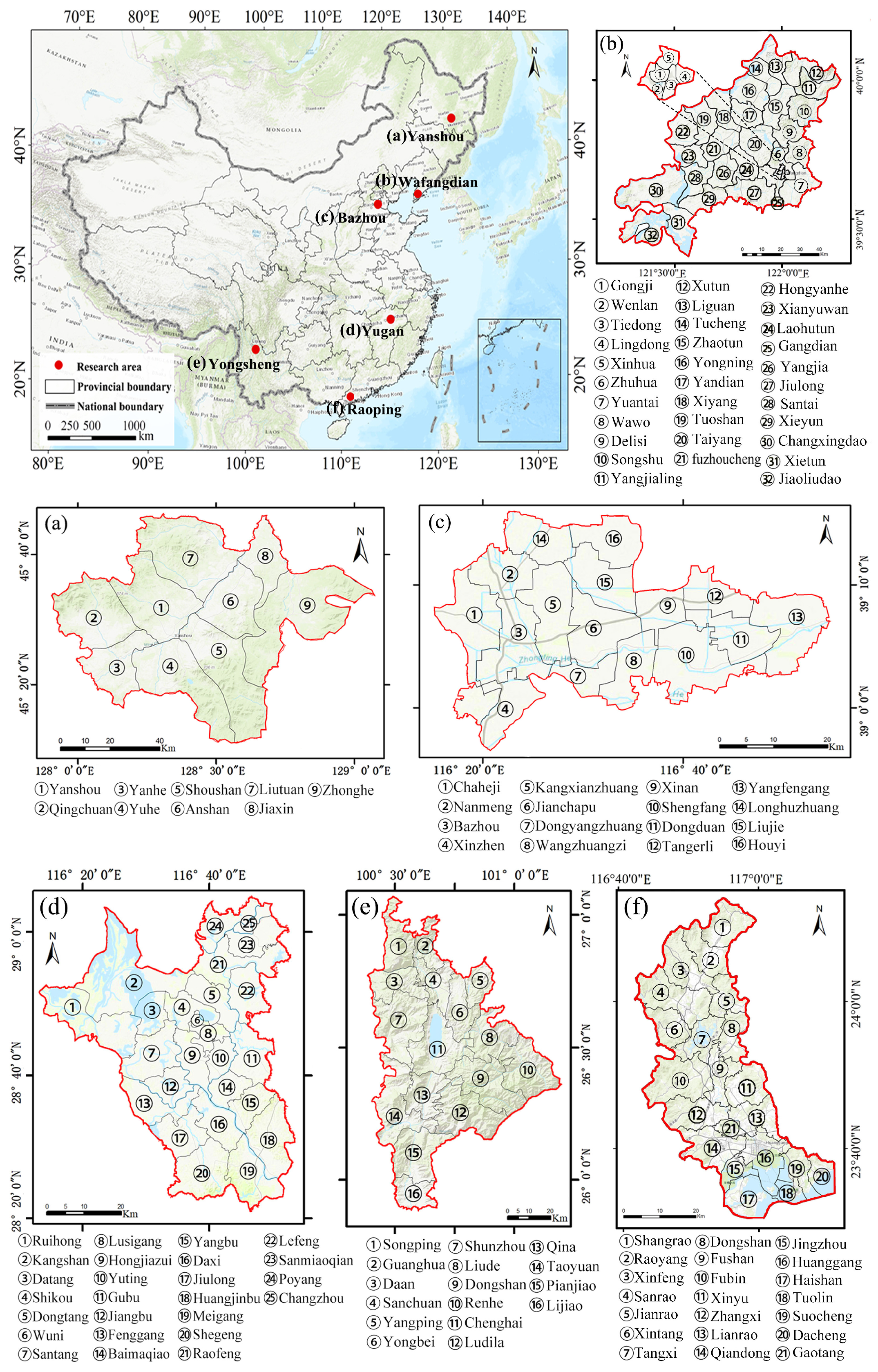
In this study, six representative counties are examined: Yanshou (Heilongjiang), Wafangdian (Liaoning), Bazhou (Hebei), Yugan (Jiangxi), Yongsheng (Yunnan), and Raoping (Guangdong) (Figure 1). Spanning China’s Northeast, North, East, Southwest, and South regions, these areas encompass diverse climatic zones (temperate to subtropical) and varied topography. The sample ensures multidimensional representativeness, including four formerly impoverished counties and two developed regions, with economies ranging from agriculture-dominant (Yanshou and Yugan) and manufacturing-driven (Bazhou and Wafangdian) to ecological-agricultural and industrially transitioning (Yongsheng and Raoping). Geographically, the study covers both coastal and inland areas, including plains and mountains. This diversified framework captures heterogeneous development patterns across China, providing a robust basis for analyzing EWB determinants across different geographic and socioeconomic contexts.

3. Data Sources

3.1. EWB Household Survey Data

Although no unified indicator system for evaluating EWB has yet been established in academia, leading international frameworks—such as the Better Life Index (BLI) [34], the Better Well-Being Index (BWI) [35], and the Organization for Economic Cooperation and Development (OECD) Guidelines for Measuring Subjective Well-Being [3]—all emphasize certain core dimensions, including income, work, house, health, and education. Building on this consensus, a survey questionnaire (Appendix A) that covers seven dimensions: income, work, house, health, education, quality of life, and happiness, was designed. This design ensured both scientific rigor and cross-study comparability.

To ensure that the survey questions could be fully understood by the respondents, after the initial draft questionnaire was designed, we distributed it to potential respondents (25 individuals) and asked them to discuss the draft, particularly whether the questions and options contained any ambiguities. On the basis of their feedback, we revised and finalized the design of the Chinese version of the sample questionnaire to ensure that it was easily understood by the respondents. The survey was conducted through in-person household visits, where investigators distributed questionnaires to the respondents and asked them to complete the forms independently. For individuals with low literacy levels, an assisted-questioning approach was adopted to minimize respondent subjectivity and improve survey accuracy.

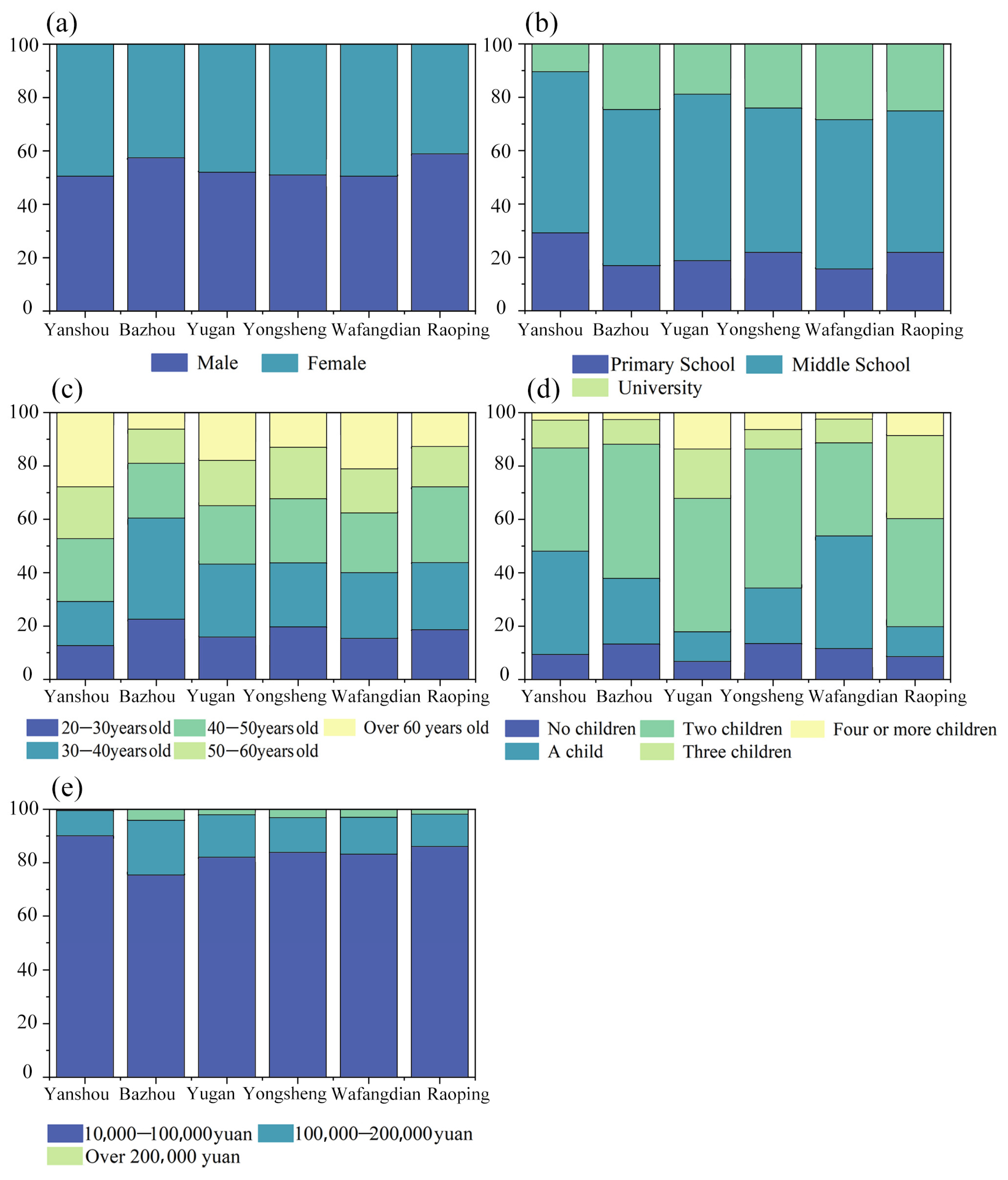
Between 18 June 2024 and 21 July 2025, household surveys were conducted across the six study regions to capture perceptions of EWB (

Table 1. Household survey data information.

Study Area	Household Survey Data	Sample Size
Yanshou	5 August to 8 August 2024	212
Wafangdian	18 July to 21 July 2025	370
Bazhou	18 June to 20 June 2024	195
Yugan	20 August to 25 August 2024	352
Yongsheng	23 December to 26 December 2024	192
Raoping	13 July to 18 July 2025	338

). In total, 119 townships were surveyed, with 10–30 respondents per township, yielding 1659 valid samples encompassing diverse demographic characteristics (Figure 2). Owing to transport constraints, Shunzhou Township in Yongsheng County could not be surveyed; to preserve spatial continuity, the data for this township were imputed using the mean values from the other surveyed townships in Yongsheng County.

3.2. Geospatial and Remote Sensing Data

To construct a comprehensive system of geographic indicators, multiple data sources, including SDGSAT-1, MOD13A3, China’s first 1 m resolution land cover, OSM, SRTM elevation, Asian housing vector and POI data, were used. The sources corresponding to each geographic indicator are detailed in

Table 2. Data source information.

No.	Data	Data Source	Data Details (Acquisition Time, Resolution)	References
1	SDGSAT-1	International Research Center of Big Data for Sustainable Development Goals (https://www.sdgsat.ac.cn/) (Accessed on 9 September 2025)	5 days, 10 m	[36]
2	MOD13A3	https://www.earthdata.nasa.gov/ (Accessed on 2 September 2025)	1 month, 1 km	[37]
3	China’s First 1 m Resolution Land Cover Data	https://zenodo.org/search (Accessed on 12 July 2025)	1 m	[38]
4	OSM Date	Open Street Map (https://www.openstreetmap.org/)(Accessed on 2 September 2025)	-	[39]
5	STRM Elevation Data	http://srtm.csi.cgiar.org/srtmdata/ (Accessed on 13 September 2025)	30 m	[40]
6	Vector Data of Houses in Asian Countries	https://doi.org/10.5281/zenodo.8174931 (Accessed on 13 September 2025)	-	[41]
7	POI Data	Gaode Map	-	[42]

.

3.3. Statistical Yearbook Data

Socioeconomic statistics were obtained from the China County Statistical Yearbook 2024, published by the National Bureau of Statistics. The key indicators for county-level development are summarized in

Table 3. Socioeconomic development indicators for counties.

Indicator (Unit)	Yanshou	Wafangdian	Bazhou	Yugan	Yongsheng	Raoping
Area (km2)	3096	3747	802	2350	4926	1746
Total resident population (person)	240,000	940,000	660,000	1,080,000	400,000	1,040,000
GDP (100 million CNY)	77	1135	452	266	124	361
The added value of primary industry (100 million CNY)	21	142	10	57	32	91
The added value of secondary industry (100 million CNY)	9	630	217	81	43	123
The added value of tertiary industry (100 million CNY)	47	363	225	128	49	147
Local General Public Budget Revenue (100 million CNY)	2.4	73	24	14	40	9.9
Local General Public Budget Expenditure (100 million CNY)	32	109	62	64	33	64
Household Deposit Balance (100 million CNY)	123	998	876	435	154	306
Number of Industrial Enterprises	49	267	285	163	18	143
Middle school students in school (persons)	6461	32,574	41,561	71,144	16,059	47,262
Primary school students in school (persons)	6868	45,939	72,653	76,209	21,466	57,450
Number of Beds in Medical and Health Institutions	1054	8734	3861	6028	1726	1792
Accommodation-Providing Social Work Institutions	14	18	13	18	5	19
Number of Beds in Accommodation-Providing Social Work Institutions	2008	4695	1187	1071	208	638
Year of poverty alleviation (year)	2020	-	-	2020	2020	2019

.

4. Method

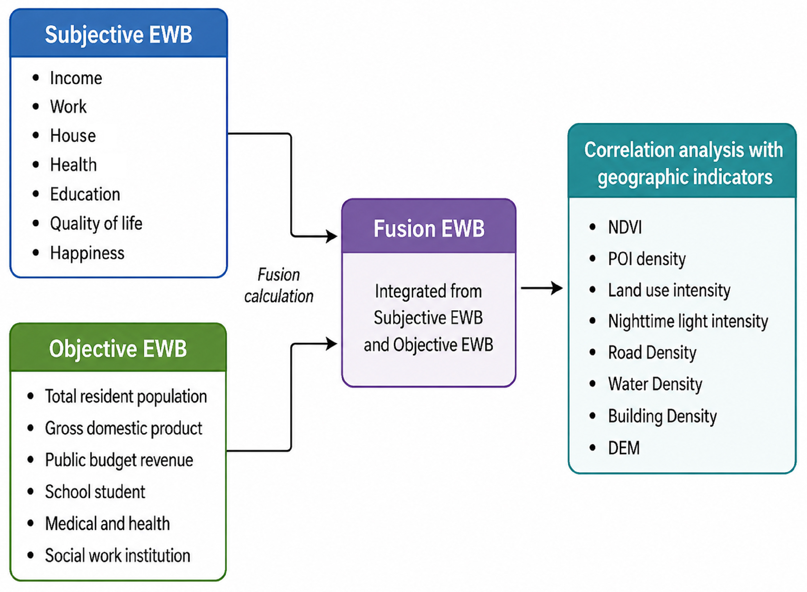
To investigate the impact of geospatial characteristics on the EWB of residents, this study introduces a three-dimensional evaluation method—subjective, objective, and fusion EWB—and analyzes how geographical environmental factors influence EWB. The three dimensions are distinguished on the basis of their data sources and analytical scales: subjective EWB is derived from household survey data that capture residents’ self-reported perceptions and satisfaction across multiple life domains; objective EWB is calculated from county-level statistical yearbook data that reflect measurable socioeconomic conditions; and fusion EWB integrates geospatial information extracted from satellite imagery and other remote sensing sources with the survey and statistical data to create a comprehensive assessment. As illustrated in Figure 3, this framework systematically connects perceptual factors (income, work, house, health, education, quality of life, and happiness) with spatial attributes (natural geography, human geography, economic activities, public services, and transport accessibility). It thereby provides a geospatial explanation for the mismatches between objective prosperity and subjective perceptions, thus extending existing theories.

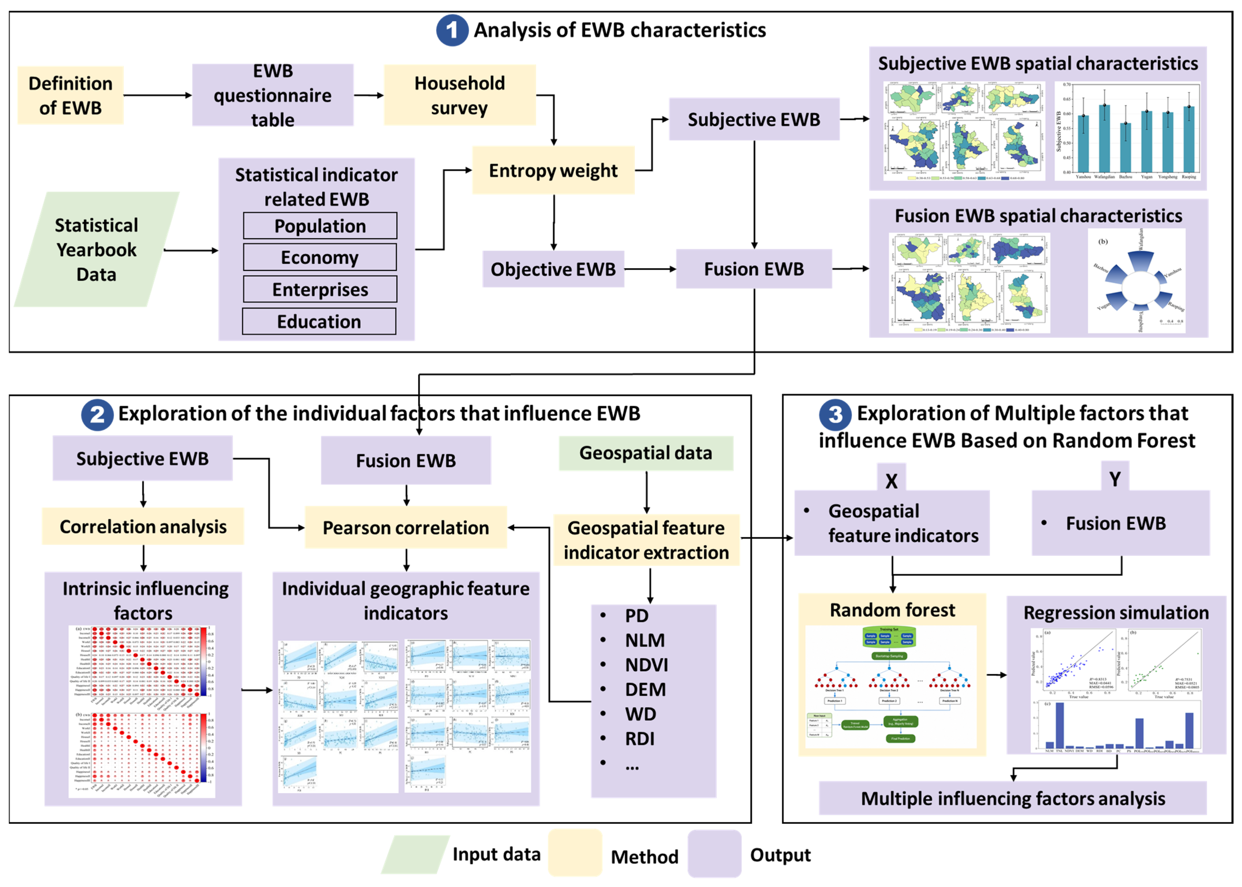
This study integrates data from household surveys, county statistical yearbooks, and remote sensing datasets. The research framework (Figure 4) comprises three components: (1) data preparation and EWB calculation (Step ①) involve calculating subjective EWB from household survey data, estimating objective EWB from county statistical data, and deriving fusion EWB by integrating both subjective and objective dimensions with geospatial features using the entropy weighting method; (2) individual-factor analysis (Step ②) involves examining how demographic and socioeconomic factors influence subjective EWB and analyzing the correlations between individual geographic indicators and both subjective and fusion EWB; and (3) multifactor modeling (Step ③) random forest algorithms are used to synthesize the relationships identified in Steps ① and ②, thereby revealing the joint effects of multiple geographic features on fusion EWB. This sequential analytical design ensures that each step builds upon the data and insights generated in the previous steps.

4.1. EWB Data Processing

(1) Processing and Calculation of Subjective EWB Data

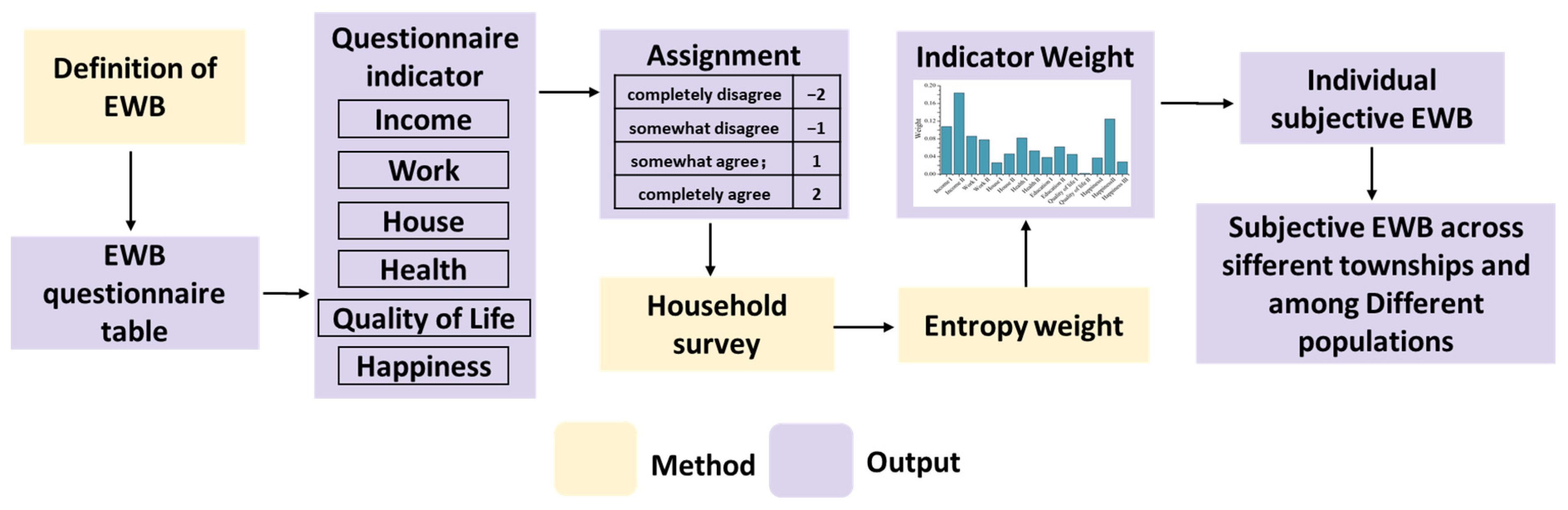
On the basis of the designed survey of residents’ subjective EWB (Appendix A), the questionnaire included basic demographic information along with seven EWB dimensions (income, work, house, health, education, quality of life, and happiness). The data processing procedure (Figure 5) was used to calculate subjective EWB at the town level.

Responses to 15 EWB-related questions were analyzed using a four-point Likert scale. The scale was used to assign scores to the responses “strongly agree,” “agree,” “disagree,” and “strongly disagree” (

Table 4. Score assignment and normalization for questionnaire options.

Questionnaire Option	Score	Assignment Normalization
completely disagree	−2	0
somewhat disagree	−1	0.25
somewhat agree	1	0.75
completely agree	2	1

). These scores were then normalized for subsequent weighting and SEWB calculations. For the questionnaire Cronbach’s α was used to test the internal consistency and reliability of the subjective EWB scale. The Cronbach’s α coefficient for the 15-item questionnaire was 0.8418, which exceeded 0.8, indicating good internal consistency of the scale.

In the entropy weight method, which is derived from information theory, indicator weights are determined by calculating information entropy, thus providing an objective measure of indicator importance [43]. Using all the survey data, we applied this method to estimate the weights of individual indicators. SEWB values for each sample were calculated on the basis of the weighted and normalized scores and were aggregated to obtain values at both the county and the town levels. The corresponding formulas are as follows:

$$SE{WB}_i=x_{i,1}\times {\omega }_1{+x}_{i,2}\times {\omega }_2\dots \dots x_{i,j}\times {\omega }_j$$

(1)

$$SE{WB}_t={\displaystyle \frac{{SEWB}_1+{SEWB}_2+\cdots +{SEWB}_n}{n}}$$

(2)

Here, $S{EWB}_i$ is the subjective EWB of the $i_{th}$ sample, $SE{WB}_t$ is the subjective EWB value of the $t_{th}$ township, $x_{ij}$ is the $j_{th}$ normalized indicator for the $i_{th}$ sample, ${\omega }_j$ is the weight of the $j_{th}$ indicator, and $n$ is the number of samples in the $t_{th}$ township.

(2) Data Processing and Calculation of Objective and Fusion EWB

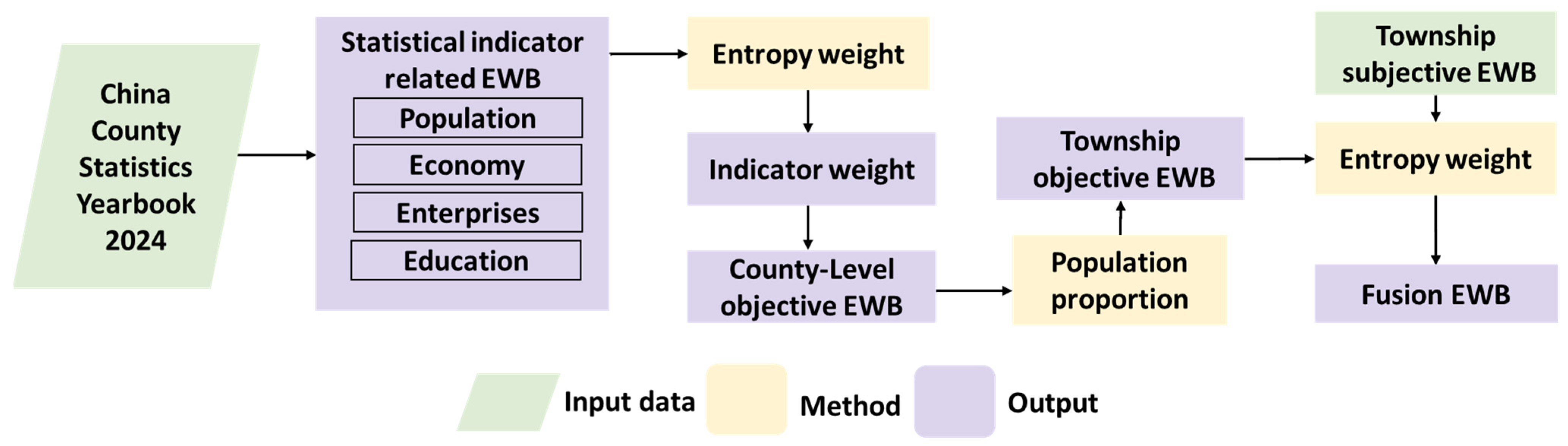
Fusion EWB was derived by integrating town-level SEWB with corresponding objective EWB values. Separate weights for subjective and objective EWB were determined using the entropy weighting method, and the fusion EWB was then computed at the town level (Figure 6). Administrative areas and the registered population were further transformed to derive population density and per capita GDP.

These indicators were weighted using the entropy weighting method to calculate county-level objective EWB (${OEWB}_i$) (

Table 5. Weights of the socioeconomic development indicators for counties.

Indicator (Unit)	Weight	Indicator (Unit)	Weight
Population density (persons/km2)	0.071	Household Deposit Balance (100 million CNY)	0.082
GDP (100 million CNY)	0.058	Number of Industrial Enterprises	0.123
The added value of the primary industry (100 million CNY)	0.03	Middle school students in school (person)	0.054
The added value of the secondary industry (100 million CNY)	0.101	Primary school students in school (person)	0.056
The added value of the tertiary industry (100 million CNY)	0.047	Number of Beds in Medical and Health Institutions	0.046
Local General Public Budget Revenue (100 million CNY)	0.111	Accommodation-Providing Social Work Institutions	0.105
Local General Public Budget Expenditure (100 million CNY)	0.047	Number of Beds in Accommodation-Providing Social Work Institutions	0.069

), as expressed by the following formula:

$${OEWB}_i=x_{i,1}\times {\omega }_1{+x}_{i,2}\times {\omega }_2\dots \dots x_{i,j}\times {\omega }_j$$

(3)

Here, ${OEWB}_i$ is the objective EWB of the $i_{th}$ county, $x_{i,j}$ is the normalized value of the $j_{th}$ indicator, and ${\omega }_j$ is the weight of the $j_{th}$ indicator.

Using population density as a scaling factor, ${OEWB}_i$ was downscaled to obtain town-level objective EWB values (${OEWB}_t$), as shown in the following formula:

$${OEWB}_t={OEWB}_c\times {\displaystyle \frac{P_{c,t}}{P_c}}$$

(4)

Here, ${OEWB}_t$ is the value for the $t_{th}$ township in the $C_{th}$ county, ${OEWB}_c$ is the objective EWB value of county C, $P_{c,t}$ is the population of the $t_{th}$ township in county C, and $P_c$ is the total population of county C.

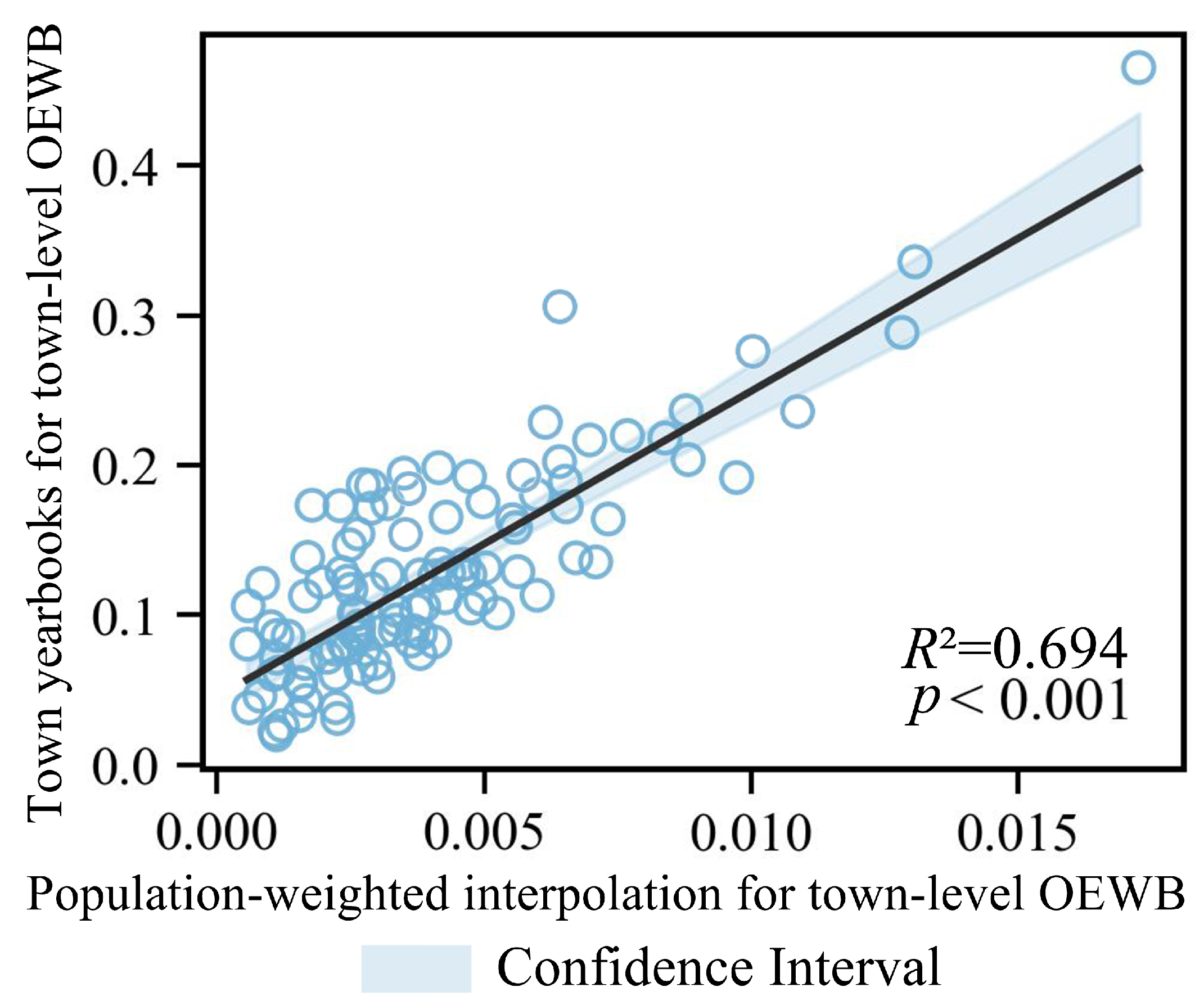
To further examine the rationality of using the population-weighted areal interpolation method for spatial downscaling, in this study, available township-level statistical yearbook data from 108 townships in six county-level areas, namely Bazhou, Yanshou, Yugan, Yongsheng, Raoping, and Wafangdian, were used after 11 subdistricts with missing data were excluded. Five available indicators were selected and weighted to calculate objective EWB at the township level. The objective EWB calculated from township-level statistical indicators was then compared with the objective EWB obtained through downscaling, and a correlation analysis was conducted to verify the rationality of using the population-weighted areal interpolation method to derive township-level objective EWB (Figure 7). Because the data are normalized during the subsequent calculation of the residents’ fusion EWB, the differences in calculation methods and units of measurement between the two objective EWB measures do not affect the subsequent calculation. Therefore, this validation mainly focuses mainly on examining the consistency of the trend and relative differences in township-level objective EWB. The changes in the downscaled objective EWB are relatively consistent with those for the objective EWB calculated from township-level statistical indicators. The correlation coefficient is R² = 0.694 (p < 0.001), indicating that the calculated objective EWB is reasonable and has good practical explanatory power.

We then recalculated the weights of the subjective and objective components via the entropy weighting method to obtain the town-level fusion EWB (${FEWB}_t$). The entropy weights of the subjective and objective EWB components were 11.4% and 88.6%, respectively, and the calculation formula is as follows:

$${FEWB}_t=SE{WB}_t\times {\omega }_s+OE{WB}_t\times {\omega }_o$$

(5)

Here, ${SEWB}_t$ and ${OEWB}_t$ are the subjective and objective EWB values for the $t_{th}$ township, and ${\omega }_s$ and ${\omega }_o$ are their respective entropy weights.

4.2. Geospatial Feature Indicator Extraction

EWB is closely linked to geographical features. We selected fifteen spatial indicators (

Table 6. Geospatial feature indicator system.

Data Source	Indicator Name	Expression	Definition	References
SDGSAT-1	Total Nighttime Light (TNL)	$TNL={\displaystyle \sum _{i=1}^n}{C}_i\times D{N}_i$	DNi is the ith gray level, Ci is the number of pixels that correspond to the gray level, and n represents the total number of pixels.	[44]
	Nighttime Light Mean (NLM)	$NLM=TNL/{\displaystyle \sum _{i=1}^n}{C}_i$	DNi is the ith gray level, Ci is the number of pixels that correspond to the gray level, and n represents the total number of pixels.
MOD13A3	Normalized Difference Vegetation Index(NDVI)	${NDVI}_i={\displaystyle \frac{(NIR-R)}{(NIR+R)}}$ $\overline{NDVI}={\displaystyle \frac{{\displaystyle {\sum }_{i=1}^n}{NDVI}_i}{n }}$	NIR denotes the reflectance of the near-infrared band and R denotes the reflectance of the red band. ${NDVI}_i$ represents the value of pixel i, and n is the total pixel count.	[45]
China’s First 1 m Resolution Land Cover Data	Percentage of Construction Land (PS)	$PS=S_{ps}/S_{total}$	$S_{ps}$ is the built-up land area of the region, and $S_{total}$ is the total area of the region.	[38]
	Percentage of Cultivated Land (PC)	$PC=S_{pc}/S_{total}$	$S_{pc}$ is the cultivated land area of the region, and $S_{total}$ is the total area of the region.
OSM Data	Road Density (RDI)	$RDI=L_{road}/S_{total}$	$L_{road}$ denotes the total road length of the region, and $S_{total}$ is the total area of the region.	[39]
	Water Density (WD)	$WD=S_{water}/S_{total}$	$S_{water}$ represents the total water surface area of the region, and $S_{total}$ is the total area of the region.
DEM Data	Elevation Standard Deviation	$S=\sqrt{{\displaystyle \frac{1}{n-1}}{\displaystyle \sum _{i=1}^n}{\left(h_i-\overline{h}\right)}^2}$	$h_i$ is the elevation value of pixel $i$, $\overline{h}$ is the average elevation of the region, and n is the pixel count of the region.	[40]
POI Data	Commercial Facility Density (${POI}_{CFD}$)	${POI}_D=N/S_{total}$	$N$ denotes the number of different POI types in the region, and $S_{total}$ is the total area of the region.	[42]
	Industrial Enterprise Density (${POI}_{IED}$)
	Public Service Facility Density (${POI}_{PSFD}$)
	Science, Education, and Cultural Facility Density (${POI}_{SEFD}$)
	Sports and Leisure Facility Density (${POI}_{SLFD}$)
	Medical and Health Facility Density (${POI}_{MHFD}$)
Vector Data of Houses in Asian Countries	Building Density ($\mathrm{BD}$)	$BD=S_{build}/S_{total}$	$S_{build}$ is the total building area of the region, and $S_{total}$ is the total area of the region.	[41]

): nighttime light mean (NLM), total nighttime light (TNL), the normalized difference vegetation index (NDVI), elevation standard deviation (DEM), water density (WD), road density (RDI), building density (BD), the percentage of cultivated land (PC), the percentage of construction land (PS), and six categories of point-of-interest (POI) density—namely commercial facility density (POI_CFD), industrial enterprise density (POI_IED), public service facility density (POI_PSFD), science, education, and cultural facility density (POI_SEFD), sports and leisure facility density (POI_SLFD), and medical and health facility density (POI_MHFD). Individual-factor analysis was used to examine the correlations between geographical feature and EWB. To further investigate the combined effects of multiple features, we employed a random forest regression model using these same fifteen indicators.

Note that in the single-factor correlation analysis (Section 5.2), the six POI subcategories were aggregated into one composite POI density indicator, resulting in nine composite indicators; in the subsequent random forest analysis (Section 5.3), the POI subcategories were disaggregated to capture category-specific effects, yielding fifteen indicators in total.

4.3. Correlation Analysis Method

Bivariate correlation analysis is a statistical method used to explore the linear relationship between two variables [19]. In this study, the Pearson correlation coefficient is used to analyze the correlation between an individual geographical feature and subjective and fusion EWB to identify key individual factors that influence EWB. The corresponding formula is as follows:

$$r={\displaystyle \frac{N{\displaystyle {\sum }_{i=1}^N}{x}_i{y}_i-{\displaystyle {\sum }_{i=1}^N}{x}_i{\sum }_{i=1}^N{y}_i}{\sqrt{N{\displaystyle {\sum }_{i=1}^N}{x_i}^2-{\left({\displaystyle {\sum }_{i=1}^N}{x_i}^2\right)}^2}\sqrt{N{\displaystyle {\sum }_{i=1}^N}{y_i}^2-{\left({\displaystyle {\sum }_{i=1}^N}{y_i}^2\right)}^2}}}$$

(6)

where $r$ is the Pearson correlation coefficient, $x_i$ is the EWB of the $i_{th}$ township, $y_i$ is the value of the corresponding geographic indicator (e.g., nighttime light intensity, road density, POI density) for the $i_{th}$ township, and N is the total number of townships.

4.4. Random Forest Method

To investigate the correlation between the fusion EWB and various geospatial characteristics, we developed a prediction model using a random forest regression approach to capture the nonlinear associations between multidimensional geospatial variables and the fusion EWB [46]. Fifteen geospatial indicators were used as input variables, including nighttime light intensity (mean and total), the NDVI, DEM, water body density, road density, building density, the proportion of built-up land, the cultivated land area, and six categories of POI density (e.g., commerce, industry, public services, education/culture, sports/recreation, and healthcare). The fusion EWB index served as the target variable. Data from 119 townships in six counties were used as observational units and randomly divided into training and validation sets (80:20 split). In the random forest algorithm, the principle of “double randomization” in ensemble learning is applied. Bootstrap resampling is employed to generate multiple independent training subsets, and at each split node, a random subset of features is selected to determine the optimal partition, thus minimizing the node-level mean squared error (MSE). The corresponding formula is as follows:

$$MSE(S)={\displaystyle \frac{1}{\left|S\right|}}{{\sum }_{i\in S}(y_i-{\overline{y}}_S)}^2$$

(7)

Here, |S| is the number of samples, $y_i$ is the true value of the sample, and ${\overline{y}}_S$ is the mean value of the sample set.

The final prediction result is calculated as the average of the outputs from B decision trees, and the corresponding formula is as follows:

$${\widehat{y}}_{RF}(x)={\displaystyle \frac{1}{k}}{\displaystyle {\sum }_{k=1}^k}{\widehat{y}}_k\left(x\right)$$

(8)

Here, ${\widehat{y}}_k\left(x\right)$ denotes the prediction of the i-th decision tree. Model accuracy was assessed using correlations between the predicted and observed values and the mean absolute error (MAE). Feature importance was quantified on the basis of the average degree of impurity reduction across trees. The model was further validated using the validation set to assess its accuracy and generalizability, and a ranked importance of geospatial features was obtained to determine their contributions to fusion EWB.

5. Results

5.1. Analysis of EWB Spatial Characteristics

(1) Analysis of the spatial characteristics of subjective EWB

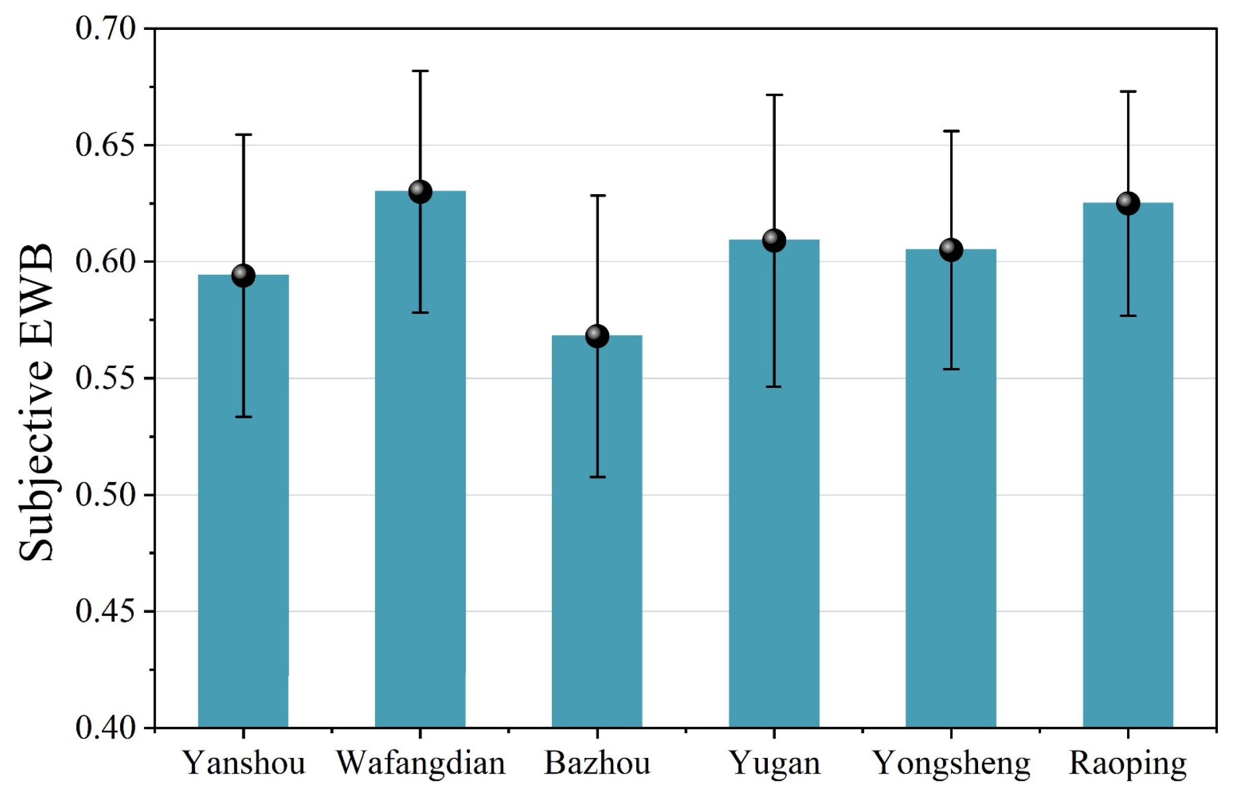
Using the entropy weighting method, indicator weights were estimated and used to calculate county-level averages of residents’ subjective EWB (Figure 8). The results show that the ranks of the six counties are as follows: Wafangdian > Raoping > Yugan > Yongsheng > Yanshou > Bazhou. A marked inconsistency was observed between subjective EWB and objective economic performance. While Wafangdian and Raoping—both economically advanced regions—exhibited high subjective EWB, Bazhou, despite outperforming the four formerly poverty-stricken counties (Yanshou, Yugan, Yongsheng, and Raoping) in terms of economic development, exhibited the lowest subjective EWB. These findings underscore that residents’ perceptions of EWB cannot be fully accounted for by economic growth alone, highlighting instead a complex nonlinear relationship between the two variables.

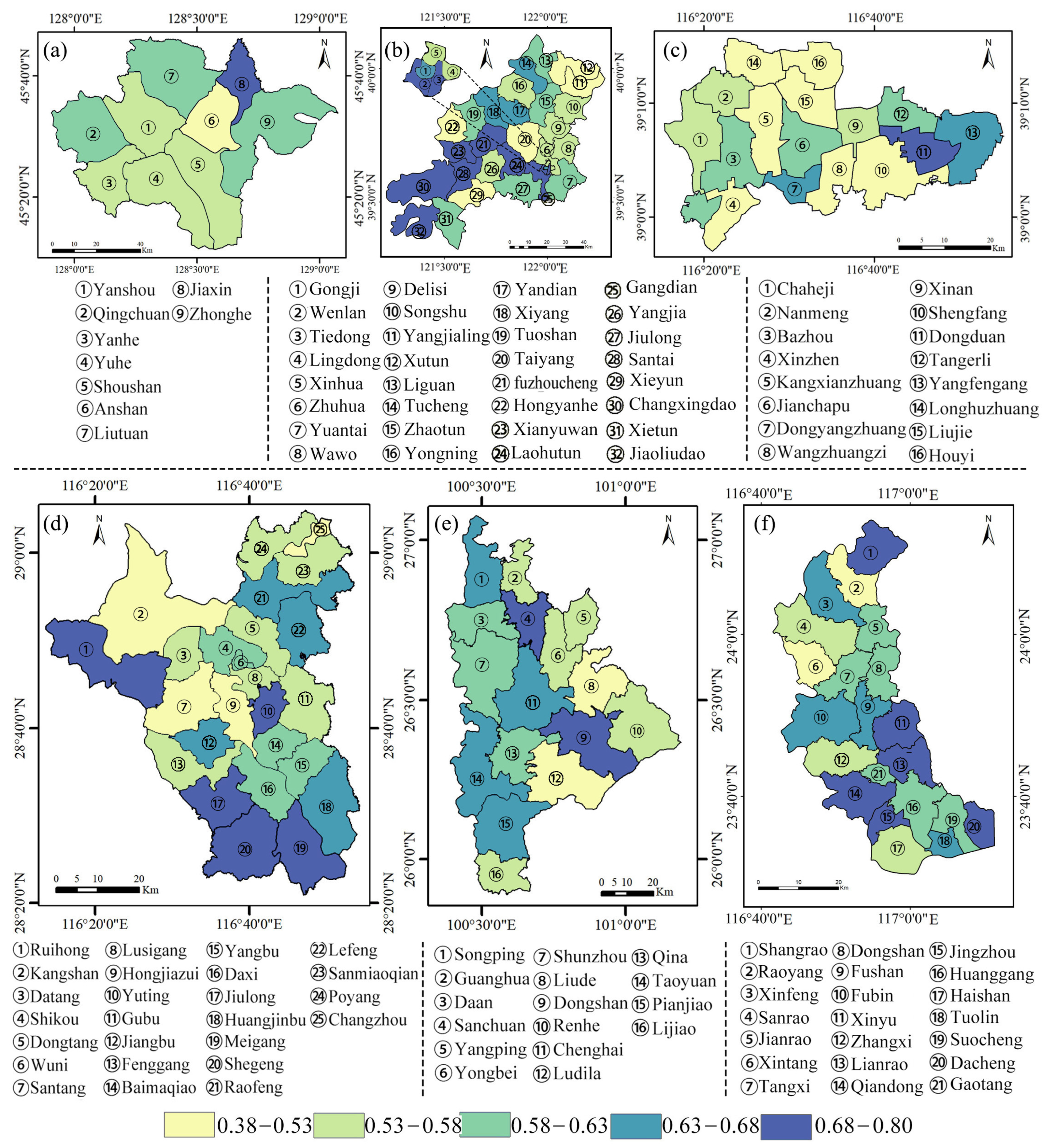
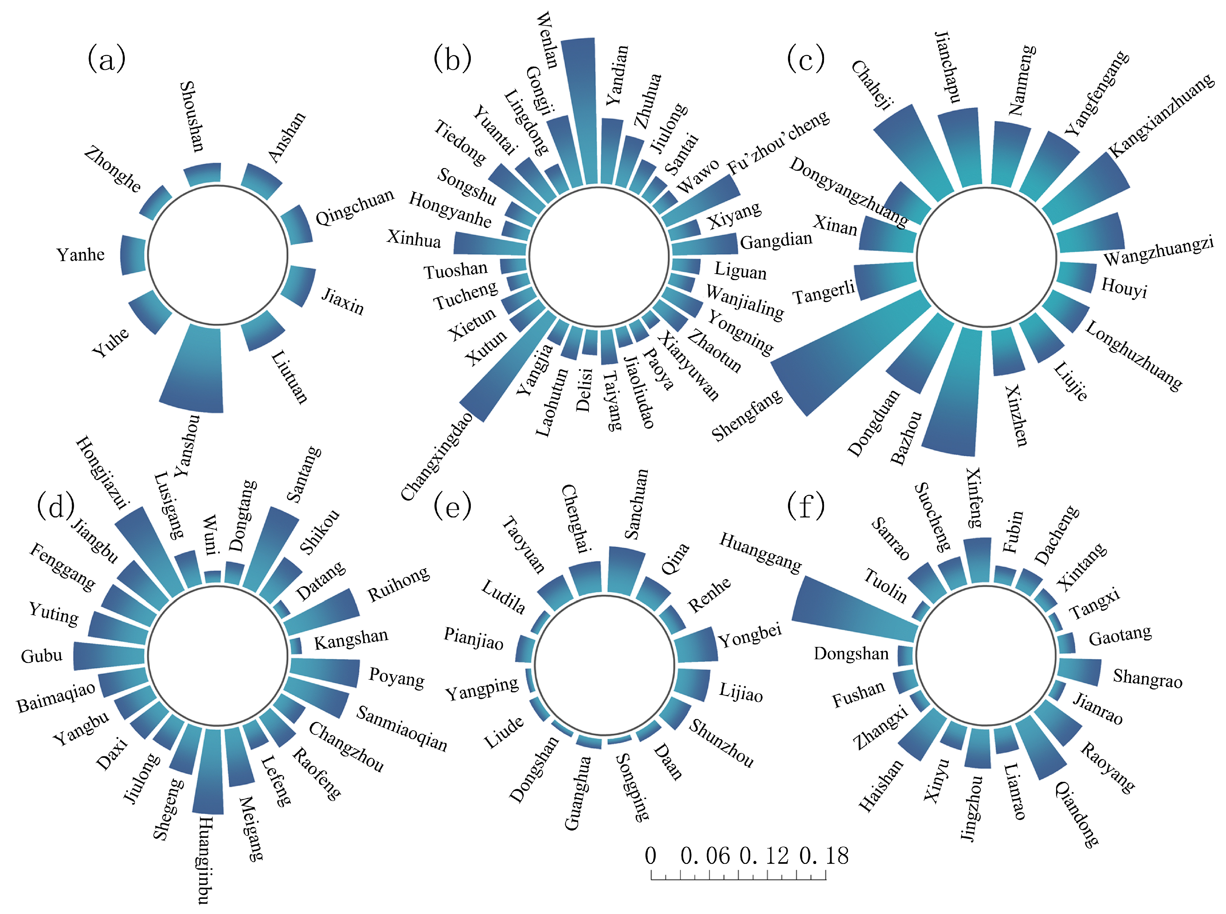
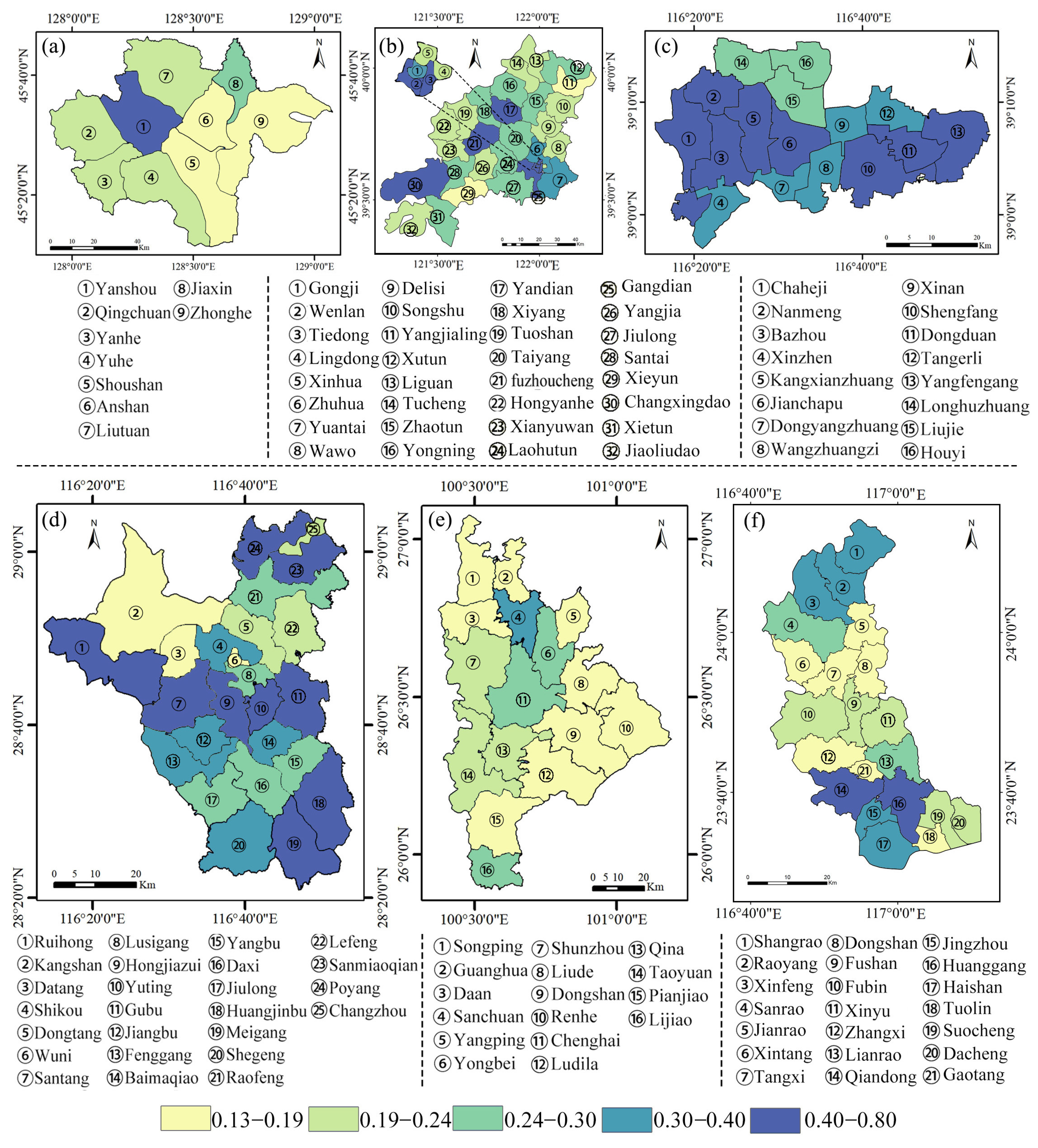
Township-level analysis further confirmed this mismatch, revealing significant spatial heterogeneity within counties (Figure 9). In Yanshou and Bazhou, most townships had relatively low subjective EWB, whereas more balanced distributions were observed in the other four counties. For instance, in Yanshou, the values for nine townships clustered in the range of 0.53 to 0.63, with that of Jiaxin being the highest and that of Anshan being the lowest. In Wafangdian, the values for 32 townships (including subdistricts) ranged between 0.58 and 0.80, with higher values along the southwestern coast and in the city center. In Bazhou and adjacent areas, the values ranged from 0.38 to 0.80, with the values in the central–northern zone being notably lower than those in other areas. Yugan (including parts of Poyang) was associated with generally higher levels, except in Kangshan, Santang, and Changzhou. In Yongsheng, the values were relatively balanced (0.53 to 0.68), with those of Sanchuan and Dongshan standing out. High levels (0.58 to 0.80) were consistently observed in Raoping, with pronounced spatial differentiation.

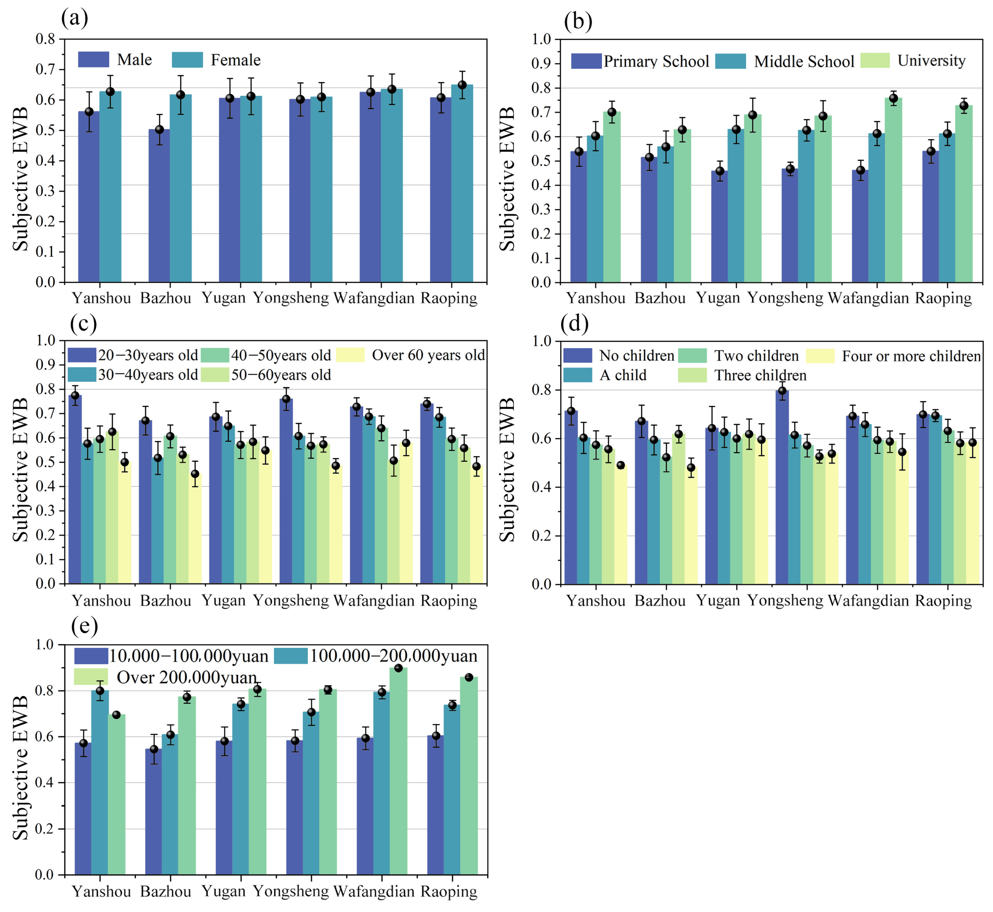
An analysis of demographic subgroups (gender, education, age, number of children, and income) revealed systematic differences in subjective EWB (Figure 10). Women generally reported higher levels of subjective EWB than men did. Subjective EWB was positively correlated with education and income but negatively correlated with age and number of children. Nonetheless, marked regional variations were observed. In Yanshou, Bazhou, and Raoping, women reported significantly higher EWB than men did, whereas gender gaps were minimal in Yugan, Yongsheng, and Wafangdian. The age effects varied: Yanshou and Yongsheng showed strong intergenerational differences; Bazhou displayed a pronounced decline among the 30–40 cohort; and Wafangdian showed an increase among residents older than 60 years. With respect to family size, although EWB generally decreased with increasing number of children, three-child families in Bazhou unexpectedly reported higher levels than other families did. These differences highlight the role of regional disparities in economic structure, work, social security, and well-being policies in shaping subjective EWB.

(2) Analysis of the spatial characteristics of objective and fusion EWB

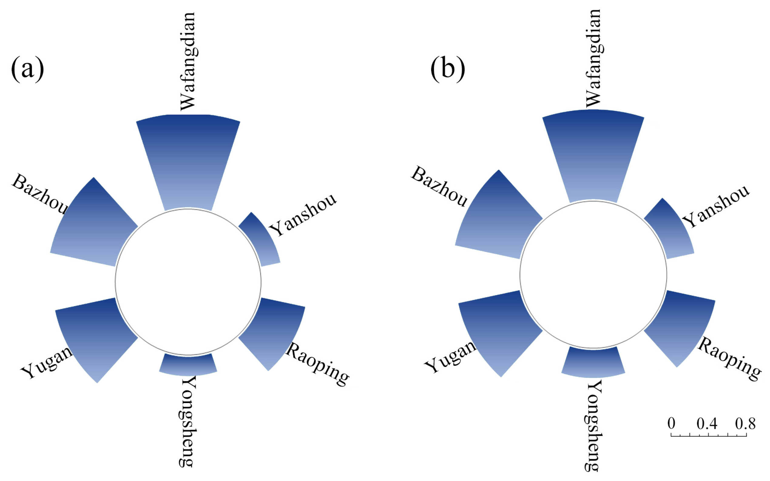
The results of the objective and fusion EWB analyses (Figure 11) revealed that the counties were ranked as follows: Wafangdian > Bazhou > Yugan > Raoping > Yongsheng > Yanshou. This ranking closely aligned with objective economic performance, thereby confirming the validity of the fusion index system. As economically advanced areas, Wafangdian and Bazhou scored highest, underscoring the critical role of economic development in shaping overall EWB.

The level of objective EWB was consistent with the level of economic development. However, the internal spatial patterns among different townships within the same county exhibited varying degrees of spatial differentiation (Figure 12).

The results at the township scale further supported this pattern, with higher fusion EWB in county seats, reflecting the positive impact of agglomeration effects (Figure 13). Spatially, Wafangdian, Bazhou, and Yugan displayed relatively high and balanced distributions; Raoping and Yanshou showed greater disparities; and Yongsheng consistently exhibited low values, reflecting the disadvantages of less developed regions. This spatial stratification provides empirical support for differentiated regional development policies.

5.2. Exploration of the Individual Factors That Influence EWB

(1) Analysis of the individual factors that influence subjective EWB

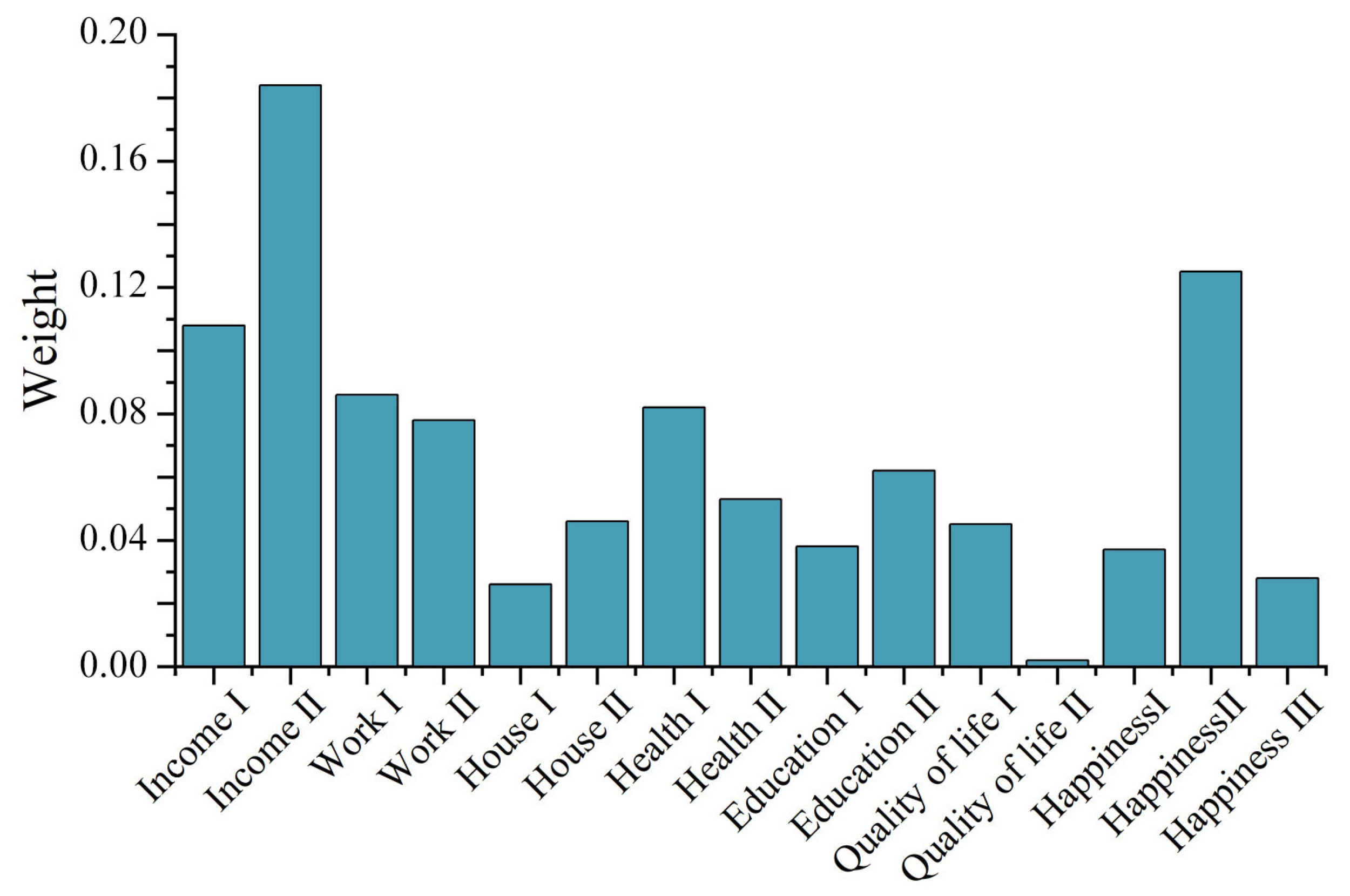
Subjective EWB was derived from residents’ survey data, which reflects individuals’ perceptions of the current level of economic development. By examining the relative weights of different indicators, the individual factors that influence subjective EWB were identified, as presented in Figure 14.

Weights were calculated using the entropy method, which assigns greater weights to indicators with greater variability. Because most EWB indicators reflected generally high satisfaction levels in the survey, those with relatively lower levels of satisfaction exhibited greater variability and thus received the highest weights, indicating that they exerted stronger effects on subjective EWB. The three highest-ranked indicators were Income II, Happiness II, and Income I, all of which are closely tied to income. Work I, Health I, Work II, and Education II also had relatively high weights, suggesting that perceived EWB related to income, work, health, and education remains relatively low and that these factors constitute major constraints on subjective EWB. In contrast, Quality of Life II, House II, and Happiness III had lower weights, indicating that residents are largely satisfied with these dimensions and do not prioritize them as areas of concern.

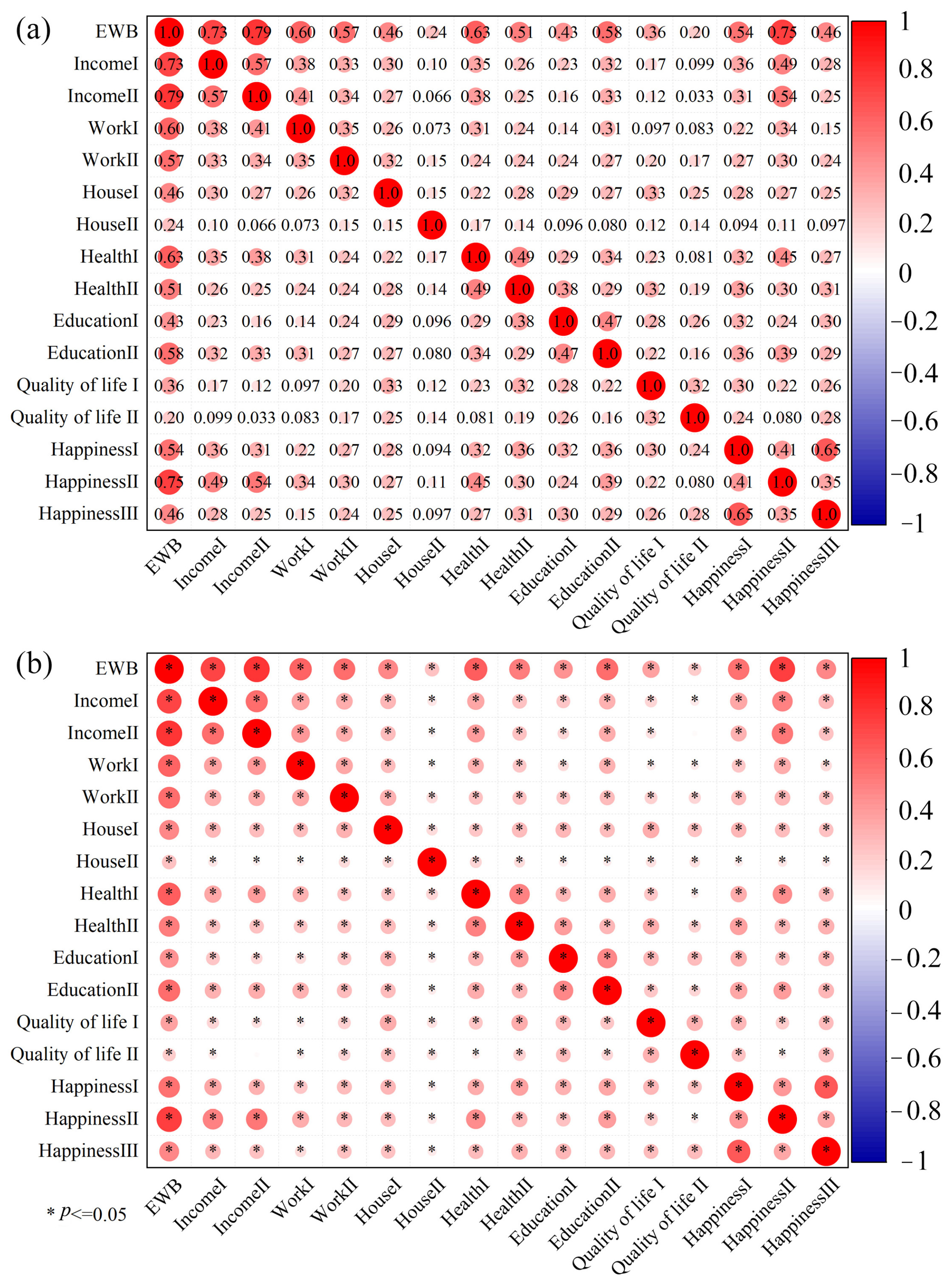
To further investigate the intrinsic factors that influence EWB, correlation and significance analyses were conducted between subjective EWB and the survey indicators (Figure 15). Subjective EWB was positively correlated with all the indicators, although the correlation strengths varied considerably. Income-related variables exhibited the strongest effects, with coefficients of 0.79, 0.75, and 0.73 for Income II, Happiness II, and Income I, respectively, establishing income as the core determinant. Work and health exhibited the next strongest effects, with Work I, Health I, Work II, and Education II having coefficients of 0.63, 0.60, 0.58, and 0.57, respectively. House II and Quality of Life II displayed weaker correlations. Significance tests confirmed that income, happiness, and several education and health indicators were significantly associated with subjective EWB (p < 0.05), whereas quality-of-life indicators were not. Combined with the entropy weighting results, these findings indicate that income, happiness, work, health, and education are strongly correlated with subjective EWB—with income displaying the strongest correlation—thereby providing empirical evidence for identifying key pathways to enhance subjective EWB.

(2) Correlation analysis between subjective EWB and individual geospatial feature indicators

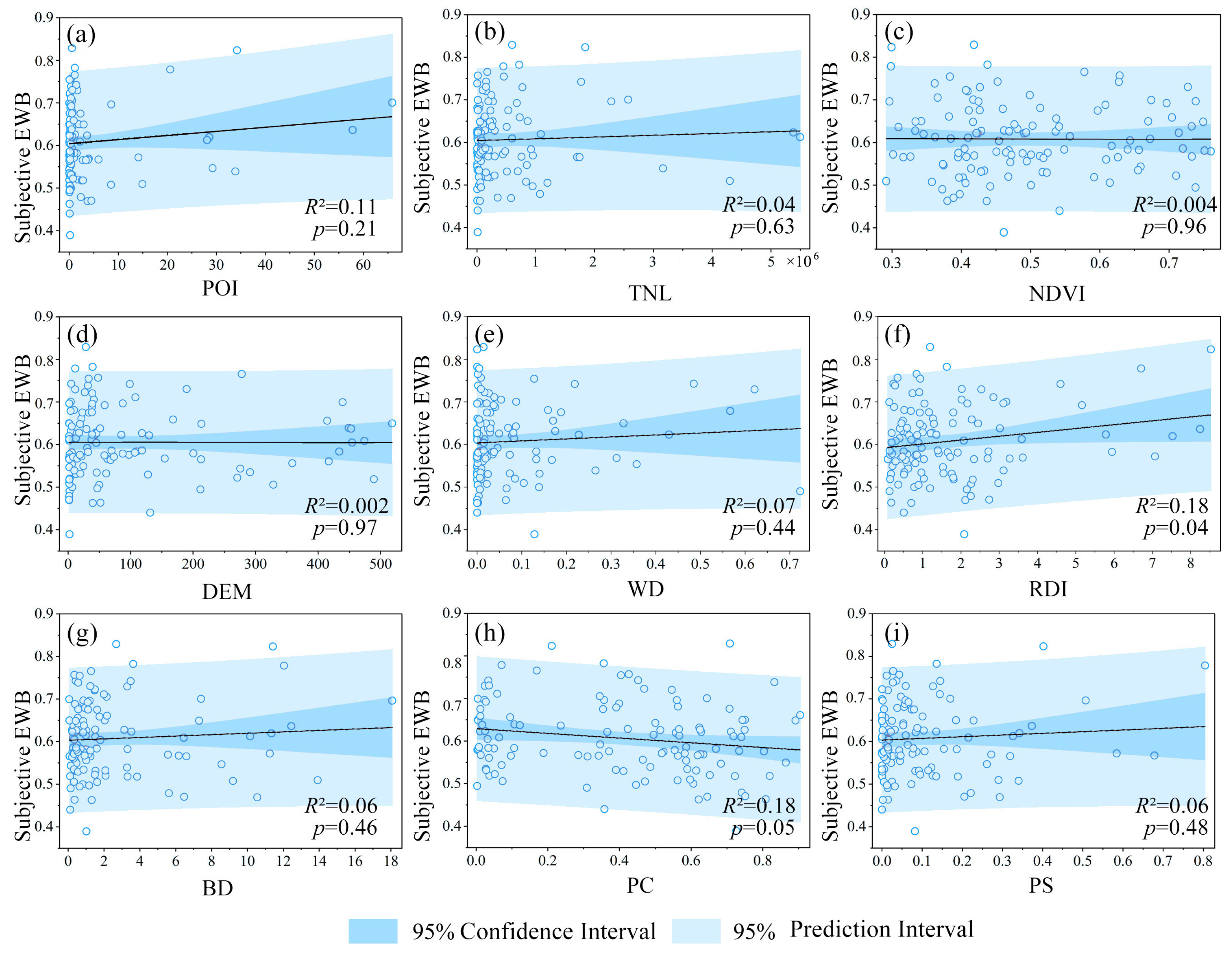
In addition to subjective perceptions, natural and human geographic factors (i.e., those related to the built and natural environments) also shape subjective EWB. Correlation analysis (Figure 16) revealed generally weak associations between nine geographic features and subjective EWB, although notable variation was observed across indicators. Road density (R² = 0.18) and POI density (R² = 0.11) were the indicators most strongly associated with subjective EWB. At the township scale, high road and POI densities indicate the presence of highly developed infrastructure. Together, these factors enhance subjective EWB by supporting work opportunities and the provision of service, confirming the positive roles of agglomeration and infrastructure development. In contrast, other factors—including total nighttime light intensity (R² = 0.04), building density (R² = 0.06), construction area (R² = 0.06), and water density (R² = 0.07)—displayed weak and statistically insignificant relationships (p > 0.1) with subjective EWB. Moreover, the NDVI (R² = 0.004) and DEM (R² = 0.002) were virtually unrelated to subjective EWB. Notably, the cultivated land area (R² = 0.18) was negatively correlated with subjective EWB, indicating that agriculture-dominated regions tend to be characterized by low levels of development and EWB, thereby underscoring the important role of the industrial structure.

(3) Correlation analysis between fusion EWB and individual geospatial feature indicators

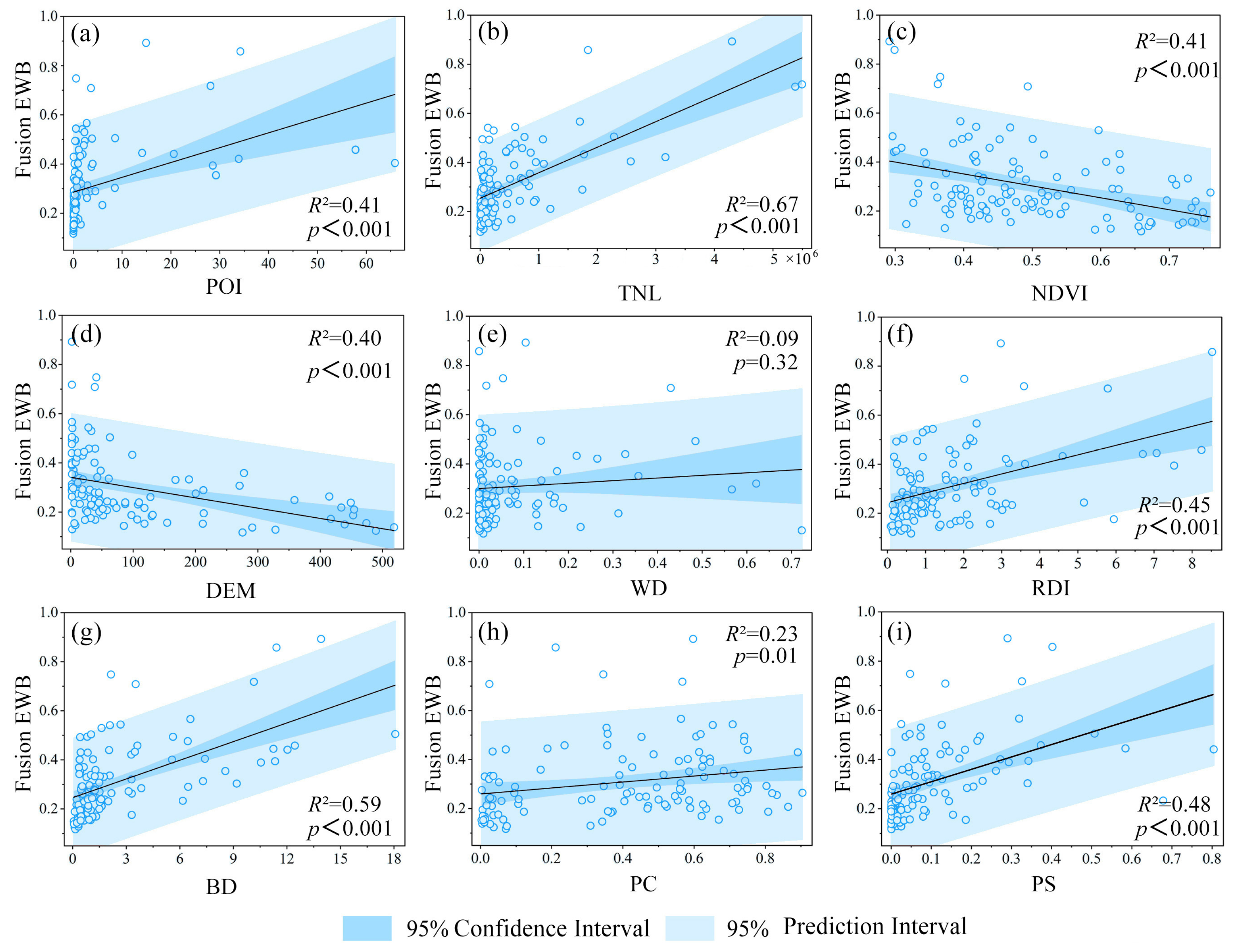
Fusion EWB, which integrates subjective perceptions with objective development, offers valuable insights for tailoring policies aimed at improving EWB. Using nine geographic features (Figure 17), we found stronger and more differentiated associations with fusion EWB than with subjective EWB alone. Specifically, the built-environment indicators were dominant: total nighttime light intensity (R² = 0.67) displayed the strongest correlation, followed by building density (R² = 0.59), construction area (R² = 0.48), road density (R² = 0.45), and POI density (R² = 0.41), thereby reflecting the central roles of urbanization and infrastructure development. Natural features exhibited a contrasting pattern: the NDVI (R² = 0.41) and DEM (R² = 0.40) were strongly negatively related to fusion EWB, suggesting that while vegetation cover and complex terrain support ecosystems, they constrain economic growth. The impacts of cultivated land (R² = 0.23) and water density (R² = 0.09) were more limited. Overall, built-environment-related factors exerted a stronger influence than natural factors did, although individual features alone provided limited explanatory power, highlighting the need for multifactor nonlinear modeling.

5.3. Exploration of Multiple Factors That Influence EWB Based on Random Forest

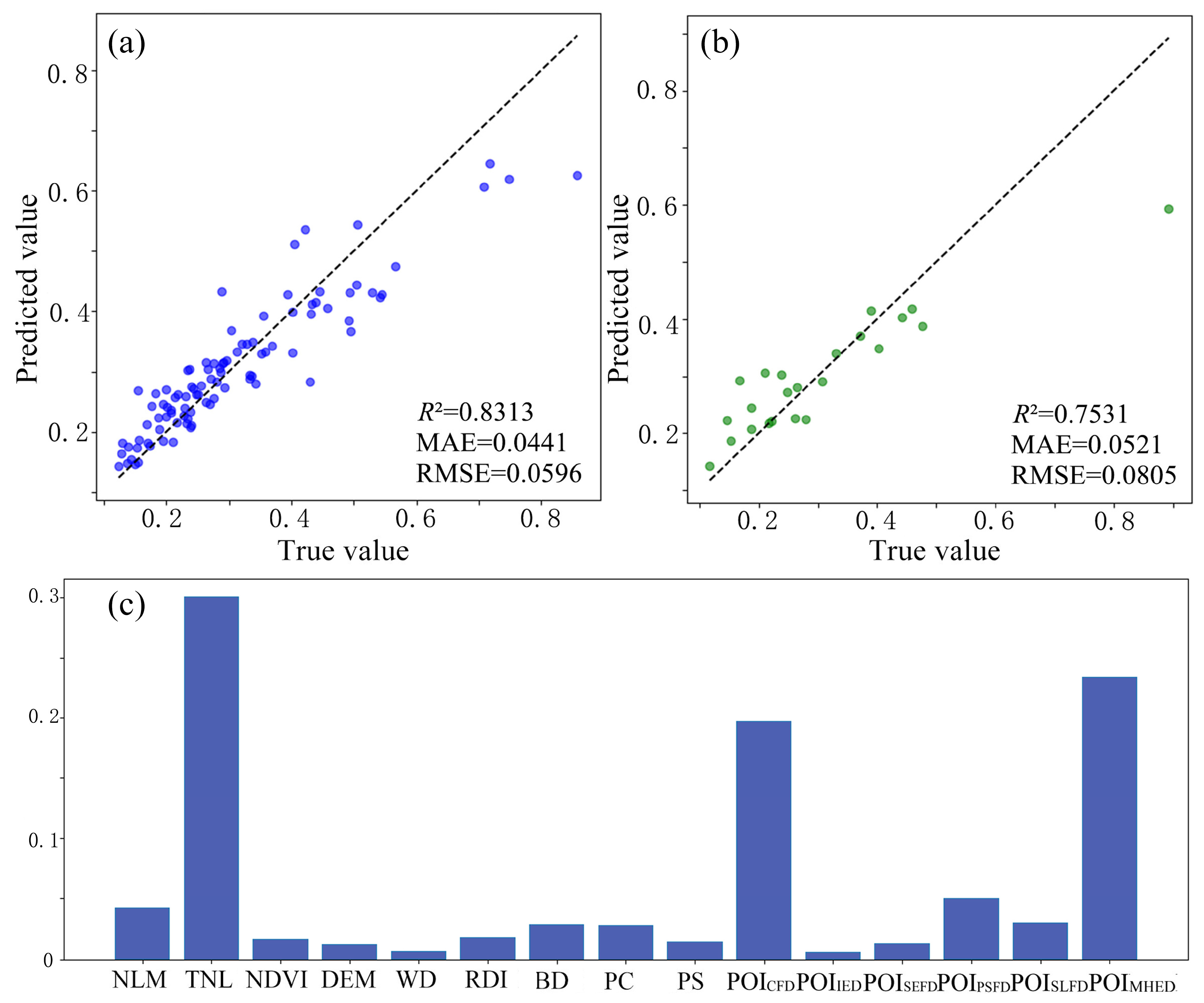
Because residents’ subjective EWB is strongly influenced by individual perceptions and satisfaction, the corresponding EWB levels exhibit high variability. On the basis of the above results regarding the relationship between individual geographical features and residents’ subjective EWB, most indicators were weakly correlated with subjective EWB, indicating that geographical characteristic indicators have limited explanatory power for subjective EWB. Meanwhile, in our previous analysis [47,48], we reported that the nighttime light intensity can effectively represent residents’ fusion EWB but not residents’ subjective EWB. Therefore, in the subsequent analysis of the synergistic effects of multiple geographical features on EWB, only residents’ fusion EWB was considered. To identify key drivers, a random forest model was constructed using 119 townships as units of analysis, incorporating 15 geographic features (average and total nighttime light intensity, NDVI, DEM, water density, road density, building density, construction land area, cultivated land area, and six POI categories). The results are shown in Figure 18. The model achieved strong performance, with R² = 0.8313 and MAE = 0.0441 for the training set, indicating its ability to characterize the synergistic effects of various spatial indicators on the fusion EWB. The validation set yielded R² = 0.7531, confirming the adequate generalizability of the model and supporting the representativeness of the geographic feature framework. A feature importance analysis revealed a layered structure of synergistic drivers: total nighttime light intensity was the most influential factor, reflecting the centrality of economic activity. Commercial and medical POI densities were also critical, underscoring the role of infrastructure availability. The public service facility density, mean nighttime light intensity, sports and leisure facility density, proportion of cultivated land, and building density further contributed to the multidimensional interactions.

The random forest model effectively captured the nonlinear and complex relationships between geographic features and the fusion EWB, indicating the primary role of built-environment-related factors and the moderating role of natural conditions. These findings provide robust evidence for forecasting EWB and formulating spatially targeted policies to enhance EWB.

6. Discussion

6.1. EWB Indicator System and Weight Determination

The EWB indicator system developed in this study demonstrates strong theoretical validity and practical relevance while also exhibiting notable innovation. This system clearly differentiates between the dimensions of subjective and objective EWB and further introduces a fusion indicator that captures the multidimensional and complex nature of the EWB concept [31]. Compared with existing indices such as the United Nations Human Development Index (HDI) and the OECD BLI, the indices in the proposed framework highlight both distinctive features and meaningful linkages. The HDI primarily emphasizes three objective dimensions—life expectancy, education, and income, whereas the BLI, despite covering 11 aspects of subjective well-being, lacks a systematic study of fusing subjective and objective dimensions [34]. The novelty of this study lies in the establishment of a household survey-based system for measuring subjective EWB, combined with a scientifically derived weighting scheme that enables the coherent fusion of subjective and objective indicators. This design provides a comprehensive and accurate tool for assessing regional EWB. Its conceptual foundation of fusing subjective and objective perspectives, along with its methodological structure, can be adapted and localized to suit diverse regional contexts. Nonetheless, the global application of this framework requires careful consideration of contextual differences. Cultural and institutional variations may influence the reporting and measurement of subjective well-being [1]. Finally, regional differences in the stages of economic development and the prevailing social values should be considered.

The entropy weighting method employed here provides strong objectivity and rigor, as indicator weights are calculated on the basis of information entropy, avoiding subjective biases inherent in expert scoring [43]. It effectively reflects cross-county differences, assigning the highest weights to income and happiness, with work-related indicators also contributing substantially—which is consistent with previous findings [12]. The mathematical foundation of the proposed method ensures reproducibility and is suitable for multi-indicator systems for analyzing complex EWB relationships. Its effectiveness was validated through random forest modeling, in which the fusion EWB strongly fitted the geospatial characteristics of the study region (R² = 0.8313).

Despite these strengths, challenges remain in applying the entropy weighting method. The method’s reliance on data variability makes it sensitive to outliers, and it may overemphasize variable indicators while underestimating substantively important indicators [49]. We employ normalization to standardize the units of measurement across all the indicators, ensuring that weight allocation occurs within a normal numerical range. Another limitation is insufficient attention to inter-indicator relationships [50], which we addressed through random forest analysis. Future research could employ hybrid weighting approaches that combine expert judgment [51], adapt weights to regional contexts, and validate robustness through sensitivity analysis.

6.2. Exploration of the Factors That Influence EWB

Conventional studies have focused on individual socioeconomic factors that shape subjective well-being [52]. However, most studies have neglected spatial dimensions and subjective–objective fusion. Our research findings reveal key factors that influence well-being across different dimensions: subjective EWB is driven by income and happiness, with work-related indicators also playing a substantial role, whereas fusion EWB is relatively strongly correlated with nighttime light intensity, building density, and built-up area. Analysis of the synergistic effects of multiple geographical features on fusion EWB revealed that total nighttime light intensity and commercial/medical POI density are particularly important factors, further corroborating the relationship between nighttime lighting levels and economic activity [20,53]. This finding highlights the dominant role of “economic vitality–public services–spatial configuration” in shaping fusion EWB.

Earlier studies of subjective EWB in human settlements relied mainly on surveys and traditional statistical methods [54]. This study breaks new ground by combining household surveys, yearbooks, and remote sensing data and applying machine learning approaches such as random forests to disentangle complex spatial relationships. The findings regarding spatial heterogeneity in EWB across urban–rural settlements provide quantitative support for the “place effect” theory, confirming the distinctive role of settlement characteristics in shaping subjective perceptions.

In addition, in this study, we did not directly incorporate socioeconomic factors into the correlation analysis. On the one hand, the purpose of this study was to explore the synergistic effects of geospatial characteristic indicators on residents’ fusion EWB and to construct a remote-sensing-based indicator system for characterizing fusion EWB. On the other hand, many of the selected remote sensing indicators are directly related to socioeconomic factors. For example, nighttime light intensity is closely associated with regional economic vitality, whereas infrastructure density, building density, and road density reflect, to some extent, the regional development level and economic conditions.

Despite its contributions, this study has several limitations. The six-county sample, while representative for county-level analysis, is narrower than the national-scale surveys conducted by Dolan et al. and Kahneman & Deaton, potentially limiting generalizability [55,56]. Second, the reliance on cross-sectional data constrains the understanding of the dynamic evolution of well-being, presenting a limitation when compared with the scope of the adaptation theories of Clark et al. [11]. Third, although random forest models have strong predictive power, their black-box nature restricts interpretability, thus limiting their theoretical depth. Moreover, although the effectiveness of the model is verified, practical explanations are not provided for geographic factors. Specifically, the effects of different factors are not clarified as linear, threshold-based, saturated, or positive only within a certain range. Closing this knowledge gap is also a key focus for our future research. By introducing structural equation modeling, we aim to further understand the geographic factors that influence EWB.

6.3. Policy Implications

Differentiated and locally adapted optimization strategies should be proposed on the basis of the geographical conditions, resource endowments, and development constraints of each surveyed county. In Yongsheng County, characterized by extensive mountainous terrain and significant topographic variation, greater efforts should be made to improve infrastructure such as transportation networks, agricultural irrigation systems, and water conservancy facilities, thereby increasing regional accessibility and agricultural production capacity. In Yanshou County and Bazhou City, priority should be given to strengthening flood protection facilities, improving drainage, flood control, and emergency management systems, and enhancing the safety and stability of residents’ living and production environments. For Yugan County and Raoping County, industrial restructuring and upgrading should be accelerated, traditional industries should be improved, diversified work opportunities should be created, and residents’ income sources should be expanded. In Wafangdian City, which has a relatively strong economic foundation, efforts should be made to consolidate existing development advantages while further optimizing public service provision, improving the quality of industrial development, and promoting urban–rural coordination to strengthen the sustained contribution of economic growth to residents’ EWB.

These county-level priorities point toward broader, multiscale policy logic. The geospatial impacts identified here offer actionable guidance for interventions across multiple governance levels. Given that subjective and fusion EWB respond to distinct spatial drivers, effective strategies must be applied at several scales simultaneously: household-scale interventions that prioritize human capital development and livelihood diversification should be implemented; settlement-level planning should be conducted to enhance built environment quality and service accessibility; and regional policies must be established to strengthen institutional frameworks and infrastructure connectivity [57]. International experience supports this multiscale approach. For example, World Bank evaluations demonstrate that integrated interventions combining infrastructure, work, and social programs yield superior livelihood outcomes [58]; UN assessments emphasize that coordinated multilevel governance accelerates poverty reduction while sustaining economic growth [59]. Crucially, geographically targeted programs in Ecuador, Madagascar, and Cambodia have demonstrated that spatially differentiated interventions can enhance both resource use efficiency and development outcomes [60].

Taken together, these findings suggest that effective policy design must move beyond uniform, county-specific measures toward a fusion framework that links local conditions to high-level governance and planning. By revealing how geographic features shape residents’ EWB through both objective and perceptual pathways, this study’s framework for analyzing EWB and the geographical factors that influence EWB provides an empirical foundation for designing place-based policies that consider local spatial contexts while advancing broader sustainable development goals. Ultimately, the governments of different regions should formulate differentiated and targeted policy measures according to their geographical features and development stages, embedded within coordinated multi-scale governance, thereby promoting the continuous improvement of residents’ EWB.

7. Conclusions

In this study, a subjective–objective fusion framework is developed to systematically examine how the spatial characteristics of settlements influence residents’ EWB. Using data from six Chinese counties, the key findings include the following: (1) subjective EWB diverges from development levels, while fusion EWB aligns with them; (2) subjective EWB is more strongly correlated with income and happiness, with work-related indicators also playing a notable role, but shows weaker spatial associations with geographical environmental characteristics, whereas fusion EWB is positively associated with nighttime light intensity and building density but negatively correlated with NDVI and elevation; (3) random forest models demonstrate strong predictive performance (training R² = 0.8313), effectively capturing nonlinear spatial–EWB relationships. The framework for analyzing EWB and geographical factors that influence EWB effectively identifies diverse geospatial determinants of EWB, providing scientific foundations and practical pathways for establishing multilevel settlement planning strategies and sustainable urban management policies.

References

1. Diener, E.; Oishi, S.; Tay, L. Advances in subjective well-being research. Nat. Hum. Behav. 2018, 2, 253–260. [Google Scholar] [CrossRef] [PubMed]
2. Costanza, R.; Hart, M.; Talberth, J.; Posner, S. Beyond GDP: The Need for New Measures of Progress. The Pardee Papers, 1 January 2009.
3. Cavalletti, B.; Corsi, M. “Beyond GDP” effects on national subjective well-being of OECD countries. Soc. Indic. Res. 2018, 136, 931–966. [Google Scholar]
4. Tang, J.; Gong, J.; Ma, W. Narrowing urban–rural income gap in China: The role of the targeted poverty alleviation program. Econ. Anal. Policy 2022, 75, 74–90. [Google Scholar] [CrossRef]
5. Fletcher, C.N.; Lorenz, F.O. Structural influences on the relationship between objective and subjective indicators of economic well-being. Soc. Indic. Res. 1985, 16, 333–345. [Google Scholar] [CrossRef]
6. Wang, L.; Long, T.; Jiang, W.; Adam, E.; Wen, C.; Jiao, W.; He, G. Economic well-being assessment: A review of traditional and remote sensing approaches. Int. J. Digit. Earth 2025, 18, 2504137. [Google Scholar] [CrossRef]
7. Kahneman, D.; Krueger, A.B. Developments in the measurement of subjective well-being. J. Econ. Perspect. 2006, 20, 3–24. [Google Scholar] [CrossRef]
8. Diener, E.; Biswas-Diener, R. Happiness: Unlocking the Mysteries of Psychological Wealth; John Wiley & Sons: Hoboken, NJ, USA, 2011. [Google Scholar]
9. Sen, A. Development as Freedom; Alfred A. Knopf: New York, NY, USA, 1999. [Google Scholar]
10. Stiglitz, J.; Sen, A.K.; Fitoussi, J. The Measurement of Economic Performance and Social Progress Revisited: Reflections and Overview; OFCE: Paris, France, 2009. [Google Scholar]
11. Clark, A.E.; Frijters, P.; Shields, M.A. Relative income, happiness, and utility: An explanation for the Easterlin paradox and other puzzles. J. Econ. Lit. 2008, 46, 95–144. [Google Scholar] [CrossRef]
12. Stevenson, B.; Wolfers, J. Subjective well-being and income: Is there any evidence of satiation? Am. Econ. Rev. 2013, 103, 598–604. [Google Scholar] [CrossRef]
13. Blanchflower, D.G.; Oswald, A.J. Is well-being U-shaped over the life cycle? Soc. Sci. Med. 2008, 66, 1733–1749. [Google Scholar] [CrossRef] [PubMed]
14. Oreopoulos, P.; Salvanes, K.G. Priceless: The nonpecuniary benefits of schooling. J. Econ. Perspect. 2011, 25, 159–184. [Google Scholar] [CrossRef]
15. Huang, Y.; Li, Z.; Wu, X.; Liang, Y.; Li, X. Mapping the stage-specific interactions in rural human settlements: A pathway to understanding rural objective well-being. Appl. Geogr. 2025, 182, 103713. [Google Scholar] [CrossRef]
16. Aslam, A.; Corrado, L. The geography of well-being. J. Econ. Geogr. 2012, 12, 627–649. [Google Scholar]
17. Bonaiuto, M.; Fornara, F.; Ariccio, S.; Cancellieri, U.G.; Rahimi, L. Perceived residential environment quality indicators (PREQIs) relevance for UN-HABITAT City Prosperity Index (CPI). Habitat. Int. 2015, 45, 53–63. [Google Scholar] [CrossRef]
18. Jiang, W.; Liu, J.; Long, T.; Liu, M.; Pang, Z.; Luo, G.; Adam, E.; Ding, X.; Cui, S.; Wen, C. Preliminary analysis of factors affecting economic well-being based on SDGSAT-1 nighttime light remote sensing and household survey data. Isprs Ann. Photogramm. Remote Sens. Spat. Inf. Sci. 2025, X-G-2025, 421–426. [Google Scholar] [CrossRef]
19. Henderson, J.V.; Storeygard, A.; Weil, D.N. Measuring economic growth from outer space. Am. Econ. Rev. 2012, 102, 994–1028. [Google Scholar] [CrossRef] [PubMed]
20. Mellander, C.; Lobo, J.; Stolarick, K.; Matheson, Z. Night-time light data: A good proxy measure for economic activity? PLoS ONE 2015, 10, e0139779. [Google Scholar] [CrossRef] [PubMed]
21. Croese, S.; Cirolia, L.R.; Graham, N. Towards Habitat III: Confronting the disjuncture between global policy and local practice on Africa’s ‘challenge of slums’. Habitat. Int. 2016, 53, 237–242. [Google Scholar] [CrossRef]
22. Yao, Y.; Liu, X.; Li, X.; Zhang, J.; Liang, Z.; Mai, K.; Zhang, Y. Mapping fine-scale population distributions at the building level by integrating multisource geospatial big data. Int. J. Geogr. Inf. Sci. 2017, 31, 1220–1244. [Google Scholar] [CrossRef]
23. Combes, P.P.; Duranton, G.; Gobillon, L.; Puga, D.; Roux, S. The productivity advantages of large cities: Distinguishing agglomeration from firm selection. Econometrica 2012, 80, 2543–2594. [Google Scholar] [CrossRef]
24. Musa, H.D.; Yacob, M.R.; Abdullah, A.M.; Ishak, M.Y. Enhancing subjective well-being through strategic urban planning: Development and application of community happiness index. Sustain. Cities Soc. 2018, 38, 184–194. [Google Scholar] [CrossRef]
25. Qu, S.; Zhang, Y.; Huang, F.; Gao, J. Assessing regional sustainability from the perspective of reconciling social-ecological resilience and human well-being: Empirical evidence from China. Appl. Geogr. 2025, 182, 103720. [Google Scholar] [CrossRef]
26. Sharifi, F.; Nygaard, A.; Stone, W.M. Heterogeneity in the subjective well-being impact of access to urban green space. Sustain. Cities Soc. 2021, 74, 103244. [Google Scholar] [CrossRef]
27. Tang, Z.; Xie, M.; Chen, B.; Xu, M.; Ji, Y. Do social and ecological indicators have the same effect on the subjective well-being of residents? Appl. Geogr. 2023, 157, 102994. [Google Scholar] [CrossRef]
28. Yang, M.; Zou, Y. Assessing environmental determinants of subjective well-being via machine learning approaches: A systematic review. Humanit. Soc. Sci. Commun. 2025, 12, 828. [Google Scholar] [CrossRef]
29. Chen, Z.; Yu, B.; Song, W.; Liu, H.; Wu, Q.; Shi, K.; Wu, J. A new approach for detecting urban centers and their spatial structure with nighttime light remote sensing. IEEE Trans. Geosci. Remote Sens. 2017, 55, 6305–6319. [Google Scholar] [CrossRef]
30. Liu, X.; Hu, G.; Chen, Y.; Li, X.; Xu, X.; Li, S.; Pei, F.; Wang, S. High-resolution multi-temporal mapping of global urban land using Landsat images based on the Google Earth Engine Platform. Remote Sens. Environ. 2018, 209, 227–239. [Google Scholar] [CrossRef]
31. Alatartseva, E.; Barysheva, G. Well-being: Subjective and objective aspects. Procedia-Soc. Behav. Sci. 2015, 166, 36–42. [Google Scholar] [CrossRef]
32. Ko, S.; Lee, D. Effectiveness of green infrastructure location based on a social well-being index. Sustainability 2021, 13, 9620. [Google Scholar] [CrossRef]
33. Yeh, C.; Perez, A.; Driscoll, A.; Azzari, G.; Tang, Z.; Lobell, D.; Ermon, S.; Burke, M. Using publicly available satellite imagery and deep learning to understand economic well-being in Africa. Nat. Commun. 2020, 11, 2583. [Google Scholar] [CrossRef] [PubMed]
34. Dias, S.; Luís, S.; Cruz, B. Measuring well-being at organizational context: Exploring the Better Life Index as a measurement tool. Soc. Responsib. J. 2024, 20, 1041–1055. [Google Scholar] [CrossRef]
35. Luthar, S.S.; Ebbert, A.M.; Kumar, N.L. The Well-Being Index (WBI) for schools: A brief measure of adolescents’ mental health. Psychol. Assess. 2020, 32, 903. [Google Scholar] [CrossRef] [PubMed]
36. Lin, Z.; Jiao, W.; Liu, H.; Long, T.; Liu, Y.; Wei, S.; He, G.; Portnov, B.A.; Trop, T.; Liu, M. Modelling the public perception of urban public space lighting based on SDGSAT-1 glimmer imagery: A case study in Beijing, China. Sustain. Cities Soc. 2023, 88, 104272. [Google Scholar] [CrossRef]
37. Zhai, Y.; Jiao, H. Risk Assessment of Urban Low-Temperature Vulnerability: Climate Resilience and Strategic Adaptations. Sustainability 2025, 17, 5705. [Google Scholar] [CrossRef]
38. Li, Z.; He, W.; Cheng, M.; Hu, J.; Yang, G.; Zhang, H. SinoLC-1: The first 1 m resolution national-scale land-cover map of China created with a deep learning framework and open-access data. Earth Syst. Sci. Data 2023, 15, 4749–4780. [Google Scholar] [CrossRef]
39. Wang, Z.; Zheng, J.; Han, C.; Lu, B.; Yu, D.; Yang, J.; Han, L. Exploring the potential of OpenStreetMap data in regional economic development evaluation modeling. Remote Sens. 2024, 16, 239. [Google Scholar] [CrossRef]
40. Jarvis, A.; Reuter, H.I.; Nelson, A.; Guevara, E. Hole-filled SRTM for the globe Version 4, available from the CGIAR-CSI SRTM 90m Database, 2008. Available online: https://srtm.csi.cgiar.org (accessed on 13 September 2025).
41. Shi, Q.; Zhu, J.; Liu, Z.; Guo, H.; Liu, M.; Liu, Z.; Liu, X. A first high-quality vector data of buildings in east asian countries based on a comprehensive large-scale mapping framework. Zenodo 2023. [Google Scholar] [CrossRef]
42. Wang, Y.; Zhang, H.; Liu, L. Does city construction improve life quality?—Evidence from POI data of China. Int. Rev. Econ. Financ. 2022, 80, 643–653. [Google Scholar] [CrossRef]
43. Zhu, Y.; Tian, D.; Yan, F. Effectiveness of entropy weight method in decision-making. Math. Probl. Eng. 2020, 2020, 3564835. [Google Scholar] [CrossRef]
44. Li, R.; Liu, M.; Zhang, B.; Jiang, W.; Jiao, F.; Sheng, H.; Liu, X. Evaluation of perception and analysis of energy saving potential of nighttime illumination in different types of residential areas: A case study of Dalian, China. Sustain. Cities Soc. 2026, 114, 107417. [Google Scholar]
45. Sousa Silva, R.; Kestens, Y.; Poirier Stephens, Z.; Thierry, B.; Schoenig, D.; Fuller, D.; Winters, M.; Smargiassi, A. Urban vegetation and well-being: A cross-sectional study in Montreal, Canada. People Nat. 2025, 7, 398–414. [Google Scholar] [CrossRef]
46. Niu, T.; Chen, Y.; Yuan, Y. Measuring urban poverty using multi-source data and a random forest algorithm: A case study in Guangzhou. Sustain. Cities Soc. 2020, 54, 102014. [Google Scholar] [CrossRef]
47. Liu, J.; Jiang, W.; Liu, M.; Long, T.; Pang, Z.; Yan, D.; Adam, E.; Wen, C.; Wang, L. Correlation Exploration Between Residents’ Economic Well-Being and Nighttime Lights; IEEE: New York, NY, USA, 2025; pp. 1–6. [Google Scholar]
48. Jiang, W.; Liu, J.; Long, T.; Liu, M.; Kawasaki, A.; Pang, Z.; Yan, D.; Shang, Y.; Adam, E.; Ding, X. Can Nighttime Light Proxy Comprehensive Economic Well-being? Evidence from China. Sustain. Cities Soc. 2026, 138, 107191. [Google Scholar] [CrossRef]
49. Chen, L.; Wang, X.; Wang, Y.; Gao, P. Improved entropy weight methods and their comparisons in evaluating the high-quality development of Qinghai, China. Open Geosci. 2023, 15, 20220570. [Google Scholar] [CrossRef]
50. Liu, Z.; Xie, Q.; Dai, L.; Wang, H.; Deng, L.; Wang, C.; Zhang, Y.; Zhou, X.; Yang, C.; Xiang, C. Research on comprehensive evaluation method of distribution network based on AHP-entropy weighting method. Front. Energy Res. 2022, 10, 975462. [Google Scholar] [CrossRef]
51. Bertin, G.; Carrino, L.; Giove, S. The Italian regional well-being in a multi-expert non-additive perspective. Soc. Indic. Res. 2018, 135, 15–51. [Google Scholar]
52. Wilson, W.R. Correlates of avowed happiness. Psychol. Bull. 1967, 67, 294. [Google Scholar] [CrossRef] [PubMed]
53. Chen, X.; Nordhaus, W.D. VIIRS nighttime lights in the estimation of cross-sectional and time-series GDP. Remote Sens. 2019, 11, 1057. [Google Scholar] [CrossRef]
54. Ballas, D. What makes a ‘happy city’? Cities 2013, 32, S39–S50. [Google Scholar] [CrossRef]
55. Dolan, P.; Peasgood, T.; White, M. Do we really know what makes us happy? A review of the economic literature on the factors associated with subjective well-being. J. Econ. Psychol. 2008, 29, 94–122. [Google Scholar] [CrossRef]
56. Kahneman, D.; Deaton, A. High income improves evaluation of life but not emotional well-being. Proc. Natl. Acad. Sci. USA 2010, 107, 16489–16493. [Google Scholar] [CrossRef] [PubMed]
57. Bai, L.; Xiu, C.; Feng, X.; Liu, D. Influence of urbanization on regional habitat quality: A case study of Changchun City. Habitat. Int. 2019, 93, 102042. [Google Scholar] [CrossRef]
58. Gillespie, N. Selected World Bank Poverty Studies: A Summary of Approaches, Coverage, and Findings; World Bank Publications: Washington, DC, USA, 1990; Volume 552. [Google Scholar]
59. Monaco, S. SDG 1. In End Poverty in All Its Forms Everywhere; Emerald Publishing Limited: Leeds, UK, 2024; pp. 15–23. [Google Scholar]
60. Elbers, C.; Fujii, T.; Lanjouw, P.; Özler, B.; Yin, W. Poverty alleviation through geographic targeting: How much does disaggregation help? J. Dev. Econ. 2007, 83, 198–213. [Google Scholar] [CrossRef]
Figure 1. Study area ((a) Yanshou; (b) Wafangdian; (c) Bazhou; (d) Yugan; (e) Yongsheng; (f) Raoping).
Ijgi 15 00305 g001
Figure 2. Proportions of different demographic characteristics for the survey samples: (a) gender; (b) educational attainment; (c) age; (d) number of children; (e) income.
Ijgi 15 00305 g002
Figure 3. Framework for analyzing EWB and geographical factors that influence EWB.
Ijgi 15 00305 g003
Figure 4. Flowchart of the technical framework of this study.
Ijgi 15 00305 g004
Figure 5. Calculation process for subjective EWB.
Ijgi 15 00305 g005
Figure 6. Calculation process for fusion EWB.
Ijgi 15 00305 g006
Figure 7. Objective EWB validation at the town level based on population-proportion downscaling.
Ijgi 15 00305 g007
Figure 8. Subjective EWB at the county-scale.
Ijgi 15 00305 g008
Figure 9. Spatial distribution of subjective EWB at the town level ((a) Yanshou; (b) Wafangdian; (c) Bazhou; (d) Yugan; (e) Yongsheng; (f) Raoping).
Ijgi 15 00305 g009
Figure 10. Residents’ subjective EWB by population group ((a) gender; (b) education; (c) age; (d) number of children; (e) income).
Ijgi 15 00305 g010
Figure 11. Objective and fusion EWB at the county-scale ((a) objective EWB; (b) fusion EWB).
Ijgi 15 00305 g011
Figure 12. Spatial distribution of objective EWB at the town level ((a) Yanshou; (b) Wafangdian; (c) Bazhou; (d) Yugan; (e) Yongsheng; (f) Raoping).
Ijgi 15 00305 g012
Figure 13. Spatial distribution of fusion EWB at the town level ((a) Yanshou; (b) Wafangdian; (c) Bazhou; (d) Yugan; (e) Yongsheng; (f) Raoping).
Ijgi 15 00305 g013
Figure 14. Calculation of the weights of each indicator in the questionnaire by the entropy weighting method (The horizontal axis indicators correspond to the survey questions in the Appendix A).
Ijgi 15 00305 g014
Figure 15. Multi-indicator correlation analysis of subjective EWB ((a) correlation analysis; (b) statistical significance analysis).
Ijgi 15 00305 g015
Figure 16. Correlation analysis between subjective EWB and individual geographic feature indicators. (ai: correlations between POI, TNL, NDVI, DEM, WD, RDI, BD, PC, PS and subjective EWB, respectively).
Ijgi 15 00305 g016
Figure 17. Correlation analysis between fusion EWB and individual geographic feature indicators (ai: correlations between POI, TNL, NDVI, DEM, WD, RDI, BD, PC, PS and fusion EWB, respectively).
Ijgi 15 00305 g017
Figure 18. Random forest-based regression simulation of fusion EWB: (a) comparison between predicted values and true values in the training set; (b) comparison between predicted values and true values in the validation set; (c) feature importance of key factors that influence fusion EWB.
Ijgi 15 00305 g018