Macro-Regional Spatial Decision Support for Geo-Distributed Data Center Siting in Europe: Regional Screening and Robustness Under Weight Uncertainty

Abstract

Digital infrastructure expansion in Europe raises a spatial planning problem: early-stage screening needs to compare regional conditions while also checking whether rankings remain stable when decision priorities change. This study evaluates 24 European Nomenclature of Territorial Units for Statistics level 2 (NUTS-2) regions for geo-distributed data center development. The 2022 decision matrix uses five Eurostat criteria: information and communications technology (ICT) specialists’ share in employment, average hourly labor cost, renewable electricity share, non-household electricity price and population density. Four criteria are national intensive proxies assigned to the selected NUTS-2 regions, while population density is directly observed at the NUTS-2 level. After a log₁₀ transformation of population density and min–max normalization, we compare the weighted sum model (WSM), TOPSIS and VIKOR across four weighting scenarios. We then apply a random-weighting audit based on Stochastic Multicriteria Acceptability Analysis (SMAA) principles, using 10,000 Dirichlet weight draws, followed by a local Dirichlet sensitivity analysis around the Balanced profile. Results show that the most stable high-performing profiles are not limited to the established FLAP-D market reference. Latvija (LV00), Stockholm (SE11), Helsinki-Uusimaa (FI1B), Eesti (EE00) and Área Metropolitana de Lisboa (PT17) form the main high-performing set across stochastic rank metrics, while several mature Western metropolitan regions remain more sensitive to cost and territorial-pressure criteria. The study provides a reproducible spatial decision support framework for macro-regional screening rather than micro-siting.

1. Introduction

Digital infrastructure has become a clear spatial issue in Europe. Recent European Commission estimates suggest that data centers in the European Union used about 70 TWh of electricity in 2024 and may reach around 115 TWh by 2030, while an earlier Joint Research Centre assessment placed EU data center electricity use at 45–65 TWh in 2022 [1,2]. This makes regional location choice more than a narrow technical or financial problem. It is also a territorial one, because labor conditions, electricity prices, renewable electricity availability and territorial pressure differ across regions and can shape the attractiveness of new digital infrastructure in very different ways.

This is particularly relevant in Europe, where digital infrastructure remains associated with a relatively small group of mature metropolitan hubs, while interest in geo-distributed capacity is extending toward a wider set of regional alternatives. For an early-stage regional comparison, the main question is not simply which region ranks first under one fixed preference structure. The more relevant issue is whether some regions remain competitive when decision priorities shift. A region that performs well only under one narrow weighting profile is analytically different from a region that stays near the top across multiple plausible priority structures.

This places the problem within the literature on geographic information systems-based multi-criteria decision analysis (GIS-MCDA) and spatial decision support. GIS-based multi-criteria decision analysis provides a structured way to compare spatial units through multiple indicators and explicit decision rules [3,4,5]. The broader spatial decision support systems literature has likewise emphasized that regional comparisons should support geographically interpretable decisions rather than produce isolated rankings alone [6]. In the more specific field of data center siting, prior MCDA studies have shown that economic, environmental and infrastructural criteria can be combined in a transparent way, yet many published applications rely on deterministic designs with fixed expert weights or a single ranking under one preference structure, without a systematic exploration of how positions change when weights are allowed to vary [7,8].

This study addresses this gap. For macro-regional digital infrastructure planning, a static ranking can be useful but incomplete. It can identify good performers under a named scenario, but it says much less about whether those positions hold when the weight structure is allowed to vary. This matters in practice because early-stage infrastructure planning rarely begins with fully stable and universally agreed priorities. Cost, talent, energy and territorial pressure may all matter, but their relative importance can shift across stakeholders and planning contexts.

This study therefore frames the problem as a spatial decision support task that evaluates not only regional performance but also regional stability under weight uncertainty. It examines 24 selected European Nomenclature of Territorial Units for Statistics level 2 (NUTS-2) regions using a five-criterion Eurostat decision matrix for 2022, the most recent year with complete coverage under the applied filters. Because regional data constraints require national proxies for several criteria, the study is explicitly positioned as a macro-regional screening framework rather than a fine-grained micro-siting tool [9]. It combines a deterministic triple-engine MCDA block with a global random-weighting audit based on SMAA principles and a local Dirichlet sensitivity layer, then places the resulting rank-based measures back onto the NUTS-2 map. This reproducible workflow uses public data and can be extended to other years and regional configurations.

The paper addresses three research questions:

RQ1. Which of the 24 selected European NUTS-2 regions show the strongest macro-regional attractiveness for geo-distributed data center development when evaluated across multiple deterministic weighting scenarios and MCDA engines?

RQ2. Which regions remain stable when the weight structure is no longer fixed but explored under global weight uncertainty and local perturbations around the Balanced profile?

RQ3. Does the integration of stochastic rank metrics into a NUTS-2 choropleth framework reveal a spatially concentrated pattern of robust regional attractiveness that deterministic rankings alone do not capture?

In this paper, FLAP-D refers to Frankfurt, London, Amsterdam, Paris and Dublin, the established European data center market reference [10]. The empirical sample includes selected FLAP-D-linked regions, while London is outside the Eurostat EU/NUTS sample used here. This makes it possible to compare mature market-linked regions with selected Nordic–Baltic, Central-Eastern and Southern alternatives within the same public-data screening workflow.

Based on this design, the paper makes two linked contributions. First, it extends regional data center screening beyond one-shot deterministic ranking by combining inter-engine comparison, global weight uncertainty and local sensitivity around a neutral baseline. Second, it shows how these outputs can be interpreted spatially through NUTS-2 choropleth mapping, anchoring the analysis in spatial decision support rather than purely methodological MCDA.

The remainder of the paper is organized as follows. Section 2 reviews the literature on GIS-MCDA, data center siting, MCDA method choice, uncertainty-aware ranking and mixed-resolution regional data. Section 3 presents the materials and methods, including the Eurostat decision matrix, preprocessing steps, deterministic engines, stochastic audit, local sensitivity analysis and visual outputs. Section 4 reports the empirical results. Section 5 discusses their methodological and spatial meaning and the main limits of the study. Section 6 concludes.

2. Literature Review

This study draws on five connected literature streams: GIS-based multi-criteria decision analysis and spatial decision support, data center siting and sustainable digital infrastructure, MCDA method choice and preprocessing, uncertainty-aware ranking and spatial sensitivity and mixed-resolution regional-data limits. Together, they support a NUTS-2-referenced, mixed-resolution screening framework for selected European regions.

2.1. GIS-MCDA and Spatial Decision Support for Regional Screening

GIS-based multi-criteria decision analysis provides a structured way to compare spatial alternatives through explicit criteria and decision rules. Early work on the integration of multi-criteria evaluation with geographic information systems showed how geographically referenced alternatives could be assessed through structured criteria rather than through a single spatial variable [11,12]. Malczewski [13] provided a book-length treatment of GIS and multicriteria decision analysis, and a later survey mapped the growth of GIS-MCDA applications and methodological developments [3]. Later geographic information science work clarified the links among spatial criteria, decision rules, visualization and planning practice [4,14]. More recent work on spatial multicriteria analysis also identifies new research frontiers linked to spatial data, uncertainty, participation and decision-support practice [5].

For the present study, this literature matters because the empirical problem is regional comparison under several spatially interpretable criteria. The alternatives are selected European NUTS-2 regions, the criteria are explicitly defined and the ranking procedures are reproducible. Spatial decision support systems (SDSS) give the broader frame for this design. Keenan and Jankowski [6] describe SDSS as a long-standing field built around geographically interpretable decision problems. Applied multicriteria SDSS (MC-SDSS) studies also show that spatial tools can inform infrastructure planning when choices depend on several criteria and on their spatial distribution [15]. This literature supports a first-stage macro-regional screening matrix while leaving parcel-level assessment to later project-specific work.

2.2. Data Center Siting, Sustainable Digital Infrastructure and Energy Context

Published data center MCDA studies often evaluate a small set of predefined candidate sites or national alternatives, usually under case-specific criteria and expert-defined weighting assumptions. Data center location has been treated in the literature as a multicriteria siting problem because it combines technical, economic, environmental and operational concerns. Covas et al. [8] proposed an MCDA approach for sustainable data center location that evaluates several dimensions rather than a single cost measure. Daim et al. [16] modeled data center site selection as a multi-criteria decision-making problem, and Kheybari et al. [17] developed a methodology for sustainable data center location selection. These studies show that data center siting fits MCDA reasoning, although many existing models work with project-specific candidate sites or expert-defined decision settings.

Recent research gives more attention to sustainability, energy and renewable resources in data center siting. Ayyildiz et al. [7] integrate renewable-energy considerations into data center location selection, and Jerleus et al. [18] examine environmental footprints in the Swedish data center service sector. Reddy et al. [19] discuss metrics for sustainable data centers, while Goiri et al. [20] connect data center placement with energy-aware internet service planning. These studies clarify why electricity price, renewable electricity and infrastructure conditions are relevant to siting analysis. They also indicate where a public-data regional screening model can complement more local or engineering-oriented approaches.

The European energy context reinforces this point. The Joint Research Centre estimates that data centers and broadband communication networks form a visible component of EU electricity use and require better data collection for policy and planning [1]. Earlier European work based on the EU Code of Conduct for Data Centre Energy Efficiency also documents trends in data center energy consumption and efficiency among participating facilities [21]. European policy documents also frame data centers as an energy-intensive digital infrastructure category that requires efficiency, reporting and planning attention [2]. Studies of European energy systems argue that data centers should be viewed in relation to efficiency, integration and policy, not only as isolated facilities [22]. Renewable electricity and energy-system integration are also active topics. Huang et al. [23] review data centers as prosumers in district energy systems, with attention to renewable integration and waste-heat reuse, and Rostirolla et al. [24] review challenges and solutions for renewable-energy integration in data centers. This body of work explains why renewable electricity share and non-household electricity price are suitable macro-regional energy criteria, while detailed grid-connection, power-purchase and engineering questions remain outside the five-criterion Eurostat matrix.

2.3. MCDA Method Choice, Ranking Engines and Preprocessing

The choice of MCDA method matters because each method aggregates criteria and ranks alternatives in a different way. Hwang and Yoon [25] provide an early reference for multiple attribute decision making and the ideal-solution logic later associated with TOPSIS. The weighted sum model (WSM), also referred to in some literature as simple additive weighting (SAW), follows a transparent additive logic, and Kaliszewski and Podkopaev [26] describe simple additive weighting as a metamodel for several MCDA approaches. TOPSIS ranks alternatives by distance to positive and negative ideal solutions. VIKOR follows a compromise-ranking logic that balances group utility and individual regret. Opricovic and Tzeng [27] show that VIKOR and TOPSIS share an ideal-solution origin but can produce different rankings because their aggregation rules differ. Behzadian et al. [28] further document the wide use of TOPSIS across decision problems.

The method choice should therefore be stated rather than treated as a neutral technical step. Wątróbski et al. [29] propose a framework for selecting MCDA methods, and Cinelli et al. [30] argue for a structured taxonomy of MCDA application choices. Comparative studies show that different MCDA methods can produce different rankings from the same decision matrix [31,32,33]. In the present study, WSM, TOPSIS and VIKOR are used as complementary deterministic engines. WSM gives an additive baseline, TOPSIS gives an ideal-distance perspective and VIKOR gives a compromise-ranking perspective. This design helps distinguish regions that perform consistently across methods from regions whose rank depends more strongly on the selected decision rule.

Preprocessing is also part of the MCDA design because criteria are measured in different units and must be placed on a comparable scale. The normalization literature shows that normalization choices can affect MCDA results, especially in distance-based methods such as TOPSIS [34,35]. Vafaei et al. [36,37] show that normalization choices and outliers can influence decision outputs, while Walesiak [38] and Bánhidi and Dobos [39] show that rankings based on composite indicators and TOPSIS can be sensitive to normalization choices and weights. Transformations before normalization may be appropriate when an indicator is strongly skewed, provided that the transformation is transparent. Zavadskas and Turskis [40] propose logarithmic normalization, Zolfani et al. [41] reanalyze multi-attribute decision-making methods (MADM) with attention to logarithmic normalization, while Podvezko and Podviezko [42] discuss how data transformation can affect multicriteria evaluation results. In the present study, population density is used as a cost-oriented territorial-pressure proxy and is transformed with log₁₀ before min–max normalization. This reduces the influence of extreme urban density values while preserving C5 as a direct NUTS-2 observation.

2.4. Weight Uncertainty, SMAA Principles and Spatial Sensitivity

A single deterministic MCDA ranking depends on the selected weight vector. The SMAA family addresses this issue by exploring the weight space when preference information is uncertain, incomplete or only partly specified. The original SMAA paper introduced stochastic multiobjective acceptability analysis as a way to identify the weights that would make each alternative acceptable or preferred [43]. SMAA-2 extended this logic by considering rank acceptability across all ranks, which is closer to discrete ranking problems [44]. Later work formalized and implemented the SMAA family and described rank acceptability indices, central weight vectors and related output measures [45,46,47].

The present study draws on this literature to define a narrower stochastic layer. The implemented procedure is a WSM-based random-weighting audit based on SMAA principles. It samples weights from a Dirichlet distribution and reports rank acceptability, expected rank and rank standard deviation. Full SMAA-2 is used here as conceptual background rather than as the implemented algorithm. The local Dirichlet analysis around the Balanced scenario is a separate sensitivity layer, not a SMAA-family output. This design is consistent with the broader MCDA uncertainty literature, which shows that uncertain weights, data and assumptions can affect rankings and should be reported transparently [48,49,50].

Spatial MCDA adds a further reason to examine sensitivity. Weight changes can alter both rank positions and the mapped pattern of results. Feick and Hall [51] examine the spatial dimension of weight sensitivity, and Feizizadeh et al. [52] develop a spatially explicit sensitivity and uncertainty approach for GIS-MCDA. Related spatial sensitivity work shows that criteria weights and spatial assumptions can shape suitability outputs in ways that should remain visible to the analyst and the reader [53,54]. The present study follows this logic by combining stochastic rank measures with NUTS-2 choropleth outputs.

2.5. Mixed-Resolution Regional Data and Local Siting Interpretation

European regional comparison often relies on the NUTS classification because it provides a common territorial frame for statistical reporting. Eurostat defines NUTS as the nomenclature of territorial units for statistics and provides the territorial framework and dataset interfaces used in this study [55,56]. In the present matrix, C5 population density is directly observed at NUTS-2 level, while C1–C4 are national intensive proxies assigned to selected NUTS-2 regions. The Eurostat records used for ICT specialists, labor cost, renewable energy share, electricity prices and population density provide a transparent public-data basis for the decision matrix [55,56].

The use of national intensive proxies in a NUTS-2-referenced matrix is a mixed-resolution design choice. It is suitable for first-stage macro-regional screening when its limits are stated clearly. Regional and composite-indicator studies show that public-data screening often depends on the spatial level at which indicators are available and on the way indicators are selected and aggregated [57,58]. Work on spatial resolution and regionalization in national-scale models also shows that results can depend on the level of spatial detail used in the model [59]. For this reason, the present study uses C1–C4 as national intensive proxies to enable cross-European macro-regional comparison, while C5 remains the direct NUTS-2 observation.

This distinction also matters for local siting interpretation. Population density is useful as a macro-regional proxy for territorial pressure and spatial competition, but it is not a direct measure of local land availability or community acceptance. Recent data center studies show that data centers can raise local governance, environmental and community questions. Sovacool et al. [60] discuss the community risks and benefits of Nordic data center development, while Sovacool et al. [61] consider policy options for more sustainable internet infrastructure. Recent work also points to local socioeconomic and environmental strain near data center development and to conflicts around proposed facilities [62,63,64].

The broader infrastructure literature supports the more general point that large facilities may face land-use, landscape, permitting and social-acceptance constraints outside dense metropolitan areas. This evidence is used cautiously here because data centers have their own technical and social profile. It supports only a bounded claim: lower population density can reduce territorial pressure in a macro-regional screening model, but it does not prove local feasibility. Evidence from other energy-infrastructure settings, including transmission-line siting in Europe, points in the same direction and shows that local acceptance can depend on factors beyond density alone [65]. In this study, C5 therefore remains a territorial-pressure proxy. Local feasibility requires parcel-level assessment using land ownership, zoning, grid connection, environmental restrictions and community consultation data.

Overall, these literature streams clarify the contribution and the limits of the revised framework. GIS-MCDA and SDSS literature provides the spatial decision-support foundation. Data center siting studies justify the treatment of data center location as a multicriteria problem. MCDA method-selection and normalization sources explain the combined use of WSM, TOPSIS and VIKOR with transparent preprocessing. SMAA and spatial sensitivity research give the basis for a stochastic audit of rank behavior under weight uncertainty. Eurostat, NUTS and composite-indicator sources explain the public-data, mixed-resolution character of the matrix. Energy and social-acceptance literature clarifies why renewable electricity, electricity prices and territorial-pressure proxies matter, while preserving the distinction between macro-regional screening and local siting approval.

The present study differs from much of the earlier literature in three ways. First, it focuses on selected European NUTS-2 regions rather than a small set of project-specific candidate sites. Second, it combines WSM, TOPSIS and VIKOR with a WSM-based random-weighting audit based on SMAA principles. Third, it maps rank stability indicators back to the NUTS-2 frame, so that uncertainty can be interpreted spatially.

Table 1. Positioning of the present study relative to the main literature streams. Note: The present study is positioned as a NUTS-2-referenced, mixed-resolution screening framework that combines a Eurostat decision matrix, WSM/TOPSIS/VIKOR comparison and a WSM-based random-weighting audit under weight uncertainty. Local site assessment falls outside the scope of this macro-regional framework.

Literature Stream	Sources	Scale/ Domain	Typical Frame	Weight/Uncertainty Role	Main Limit	Present-Study Positioning
GIS-MCDA/SDSS foundations	[3,4,6,11,12,13]	Regional planning	GIS-MCDA, MCE, SDSS	Often fixed weights; sensitivity varies	General spatial support	Applies the logic to NUTS-2-referenced data center screening
Data center MCDA siting studies	[7,8,16,17]	Candidate sites or national cases	ELECTRE, AHP, TOPSIS, VIKOR and other MCDA variants	Mostly expert or method-derived weights	Often case-specific	Uses Eurostat criteria for cross-European macro-regional screening
MCDA method-selection literature	[25,27,29,30,32]	General decision problems	WSM/SAW, TOPSIS, VIKOR and other methods	Depends on method setup	Limited spatial or data center focus	Uses three engines to expose method-dependent ranking behavior
SMAA and stochastic MCDA	[43,44,45,47,48,50]	Discrete alternatives	SMAA, SMAA-2, stochastic simulation	Full SMAA-family methods explore incomplete weights; the audit samples weights for WSM scoring	Broader than the implemented audit	Uses WSM-based rank acceptability logic without full SMAA-2 outputs
Spatial sensitivity literature	[51,52,53,54]	GIS-MCDA maps and suitability models	Spatial uncertainty and weight sensitivity	Explicit sensitivity analysis	Often applied to environmental suitability	Maps rank stability and dispersion at NUTS-2 level
Eurostat/NUTS and regional indicators	[55,56,57,58,59]	European territorial units	Public regional and national datasets	Not an MCDA method	Data availability differs by indicator and level	Uses national intensive proxies with one direct NUTS-2 observation
Normalization and preprocessing	[34,35,36,37,39,40,42]	Decision matrices and composite indicators	Min–max, vector and logarithmic transformations	Normalization affects ranks	Does not define siting criteria	Documents preprocessing choices, including log10(C5)
EU energy and renewable-electricity context	[1,2,21,22,24]	EU and national energy systems	Energy-use reporting and policy analysis	Not a ranking method	Often system-level	Frames C3 and C4 as macro-regional energy criteria
Local governance, land-use and social acceptance context	[60,61,62,63,64,65]	Local communities and infrastructure sites	Case studies and governance analysis	Not an MCDA engine	Data center evidence and broader analogies require separation	Frames C5 as a proxy, not proof of local feasibility

summarizes this positioning relative to the main literature streams and lists representative sources for each stream. Section 3 presents the materials and methods and shows how these streams inform the empirical design.

3. Materials and Methods

3.1. Research Design and Analytical Workflow

This study applies a spatial decision support framework to the comparative assessment of 24 selected European NUTS-2 regions as screening units for geo-distributed data center and IT infrastructure development [55,56]. The study examines a purposive sample of 24 NUTS-2 regions selected to represent the main economic and geographical segments of the European digital infrastructure market, from established Western metropolitan cores to Nordic–Baltic markets with favorable energy and cost conditions and emerging Central, Eastern and Southern European alternatives. Regional selection was constrained by data availability: only regions for which a complete five-criterion matrix could be populated from Eurostat for the 2022 baseline were retained, which ensures internal consistency across all analytical stages.

The analytical focus is not limited to a single static ranking. Instead, the study examines how regional positions behave under alternative priority structures and under broader weight uncertainty. In this sense, the paper treats regional attractiveness as a spatial decision support problem that explicitly examines stability under weight uncertainty rather than as a one-shot ranking exercise [3,4,6].

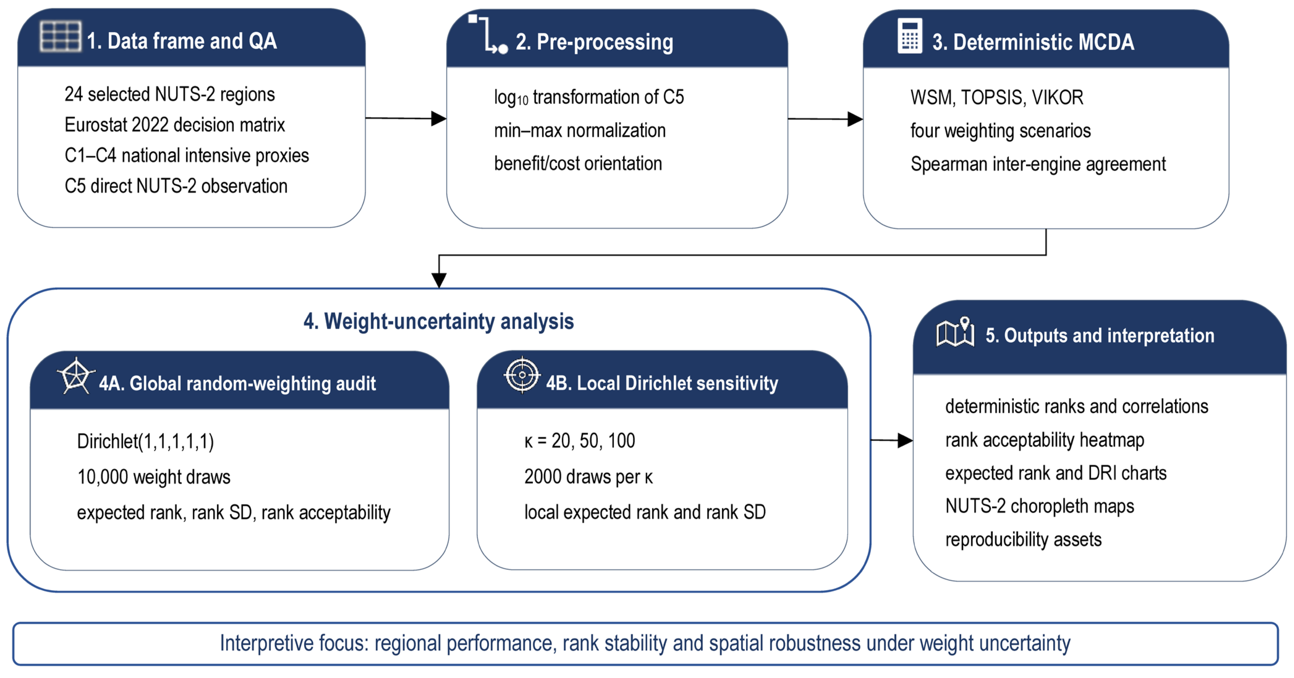
The study therefore adopts a multi-stage analytical workflow. First, a validated 24 × 5 decision matrix was constructed for the year 2022 using Eurostat data for the selected NUTS-2 regions. Second, the matrix was pre-processed through a criterion-specific transformation and a unified normalization procedure. Third, deterministic rankings were generated with three established MCDA engines, namely the weighted sum model (WSM), the Technique for Order of Preference by Similarity to Ideal Solution (TOPSIS) and the VIKOR compromise-ranking method, under four predefined weighting scenarios. This block was used to test whether the ordering of regions remained broadly consistent across different aggregation logics and priority profiles. Fourth, the analysis moved from fixed scenarios to a global stochastic audit under weight uncertainty. In that stage, repeated weight draws over the full simplex were used to estimate expected rank, rank dispersion and rank acceptability patterns for each region, following the rank-acceptability logic of SMAA [43,44,45]. Fifth, a local Dirichlet sensitivity layer was added around the Balanced scenario in order to examine how rankings behave when the analysis is centered on a neutral preference profile but allows controlled variation around it.

This design serves two purposes. At the methodological level, it separates performance from stability. A region may obtain a favorable rank under one scenario and still be unstable when the weight structure changes [48,52,54]. At the applied level, it supports a spatial reading of the results by linking stochastic rank behavior to regional maps and comparison plots. The final output is therefore not only a list of regions ordered from best to worst, but a set of spatially interpretable robustness outcomes that show where strong performance is persistent and where it is conditional on narrow preference assumptions. The overall workflow is summarized in Figure 1.

3.2. Decision Criteria and Data Sources

The analysis is based on five criteria derived from Eurostat for the reference year 2022. The selected indicators were chosen to represent a macro-regional feasibility perspective rather than a micro-siting engineering perspective. In other words, the matrix was designed to compare the broad structural attractiveness of regions for digital infrastructure development, not to model parcel-level suitability or plant-level technical design. The five criteria capture labor conditions, energy conditions and territorial pressure, which together form a plausible first-stage screening set for cross-regional comparison.

The spatial units are selected Nomenclature of Territorial Units for Statistics level 2 (NUTS-2) regions. NUTS-2 regions are medium-scale European statistical regions used for territorial reporting and comparison. In this study, they serve as the regional reference units for screening and mapping, not as parcel-level site locations.

C1 measures the share of information and communications technology (ICT) specialists in total employment and is used as a benefit criterion. It was extracted from the Eurostat dataset Employed information and communications technology (ICT) specialists (isoc_sks_itspt), using unit PC_EMP [66]. The purpose of this variable is to approximate the depth of the ICT labor base in the wider economy. It was preferred to sector-specific or narrower employment indicators because the article targets the macroeconomic capacity of a region to support digital infrastructure activity rather than the internal composition of ICT firms alone.

C2 measures average hourly labor cost and is treated as a cost criterion. It was extracted from the Eurostat dataset Labour cost levels by NACE Rev. 2 activity (lc_lci_lev), using annual euro values for 2022 and the aggregate B-S excluding O [67]. NACE Rev. 2 is the European classification of economic activities. The selected aggregate covers industry, construction and services, while excluding public administration, defense and compulsory social security. In the present context, the indicator acts as a proxy for labor-related operating cost.

C3 measures the share of renewable energy in electricity and is used as a benefit criterion. It was extracted from the Eurostat dataset Share of energy from renewable sources (nrg_ind_ren), with unit PC and energy-balance filter REN_ELC [68]. This formulation is more appropriate for the paper than the broader renewable share across all energy uses because the operational relevance for data center infrastructure lies primarily in electricity supply rather than in transport or heating. The indicator therefore works as a macro-level proxy for greener electricity conditions.

C4 measures the price of electricity for non-household consumers and is treated as a cost criterion. It was extracted from the Eurostat dataset Electricity prices for non-household consumers-bi-annual data (nrg_pc_205), using siec = E7000, nrg_cons = MWH500-1999, tax = X_VAT, currency = EUR and unit = KWH [69]. Because the Eurostat series is semi-annual, the 2022 value used in the decision matrix was constructed as the arithmetic mean of 2022-S1 and 2022-S2. This provides a transparent annual proxy aligned with the study year.

C5 measures population density and is treated as a cost criterion. It was extracted directly at NUTS-2 level from the Eurostat dataset Population density by NUTS 2 region (tgs00024), with unit PER_KM2 [70]. In this study, population density is not interpreted as a direct engineering constraint. It is used as a macro-regional proxy for territorial pressure, land scarcity and the likelihood of higher spatial competition in very dense metropolitan environments. Because C5 is cost-oriented, lower population density receives a higher normalized utility within the screening model.

A key methodological issue concerns spatial resolution. For C1–C4, the selected Eurostat filters provided complete values at national level but not consistently at NUTS-2 level for all 24 selected regions. National values were therefore assigned to the selected NUTS-2 regions within the same country. These four indicators are intensive variables: ratios, percentages, unit prices or hourly cost values. This avoids duplication of national totals and does not create artificial size effects across regions. The same logic would not be acceptable for extensive variables such as total employment, total electricity consumption or absolute ICT headcounts, and such variables were avoided in the present design. At the same time, the model does not measure within-country variation in ICT labor availability, labor cost, renewable electricity conditions or electricity prices. For countries represented by two regions in the sample, such as Germany and Romania, C1–C4 take the same national value for both selected NUTS-2 units.

By contrast, C5 is the only criterion observed directly at NUTS-2 level. No national proxy was used for this variable. For same-country region pairs in the sample, C5 is therefore the criterion that differentiates the two selected regions within the decision matrix.

Taken together, the five criteria form a compact and transparent decision matrix that is well suited to a European regional screening exercise. At the same time, the mixed-resolution design means that C1–C4 support cross-country and selected-region comparison, but not fine within-country discrimination.

3.3. Pre-Processing and Normalization

Before the ranking stage, the raw decision matrix was transformed into a common analytical format. This step was necessary because the five criteria are expressed in different units and follow different empirical distributions. Without a harmonized preprocessing pipeline, the resulting scores would partly reflect scale incompatibilities rather than the substantive contribution of each criterion to regional attractiveness.

A logarithmic transformation was applied only to C5. The reason is empirical and straightforward. Population density shows a much stronger right-skew than the other variables, with a few capital or highly urbanized regions far above the rest of the sample. If the raw C5 values were normalized directly by a linear min–max rule, the most extreme dense regions would dominate the range and compress many intermediate cases into a narrow interval. To reduce this distortion, we used log₁₀(C5) before normalization. This preserves the ordering of regions, reduces the leverage of extreme density values and improves discrimination across the middle of the distribution. The choice is consistent with the broader literature that shows how normalization results can change when indicators are highly skewed or contain strong outliers [34,35,36].

After the logarithmic adjustment of C5, all criteria were rescaled to the [0, 1] interval using a min–max transformation. For benefit criteria, that is C1 and C3, the normalized value of region i on criterion j is given by:

$$u_{ij}={\displaystyle \frac{x_{ij}-{\mathrm{m}\mathrm{i}\mathrm{n}}_i{x}_{ij}}{{\mathrm{m}\mathrm{a}\mathrm{x}}_i{x}_{ij}-{\mathrm{m}\mathrm{i}\mathrm{n}}_i{x}_{ij}}}$$

(1)

For cost criteria, that is C2, C4 and the log-transformed C5, the direction is reversed:

$$u_{ij}={\displaystyle \frac{{\mathrm{m}\mathrm{a}\mathrm{x}}_i{x}_{ij}-x_{ij}}{{\mathrm{m}\mathrm{a}\mathrm{x}}_i{x}_{ij}-{\mathrm{m}\mathrm{i}\mathrm{n}}_i{x}_{ij}}}$$

(2)

In Equations (1) and (2), x_ij is the observed value for region i on criterion j. The terms min_ix_ij and max_ix_ij denote the lowest and highest observed values of criterion j across the 24 regions. The normalized value u_ij has the same interpretation for all criteria: higher u_ij values indicate a more favorable regional outcome. This common direction is obtained directly for benefit criteria and after reversal for cost criteria.

This common interpretation is useful for two reasons. First, it keeps the input to the deterministic and stochastic blocks transparent and easy to inspect. Second, it helps ensure that differences across methods reflect differences in aggregation logic and preference structure rather than avoidable incompatibilities in raw scale representation.

The choice of min–max normalization was made for transparency and interpretability in the present study. The research literature shows that normalization choice can affect ranking outcomes, especially in methods such as TOPSIS, where normalization is structurally embedded in the scoring procedure [27,34]. In our present study, min–max normalization was retained as a simple common upstream layer for all criteria after the targeted log correction on C5. This produces a coherent analytical matrix for the subsequent multi-engine comparison and the stochastic robustness audit.

3.4. Deterministic Triple-Engine MCDA

Deterministic MCDA methods translate a decision matrix into a complete rank ordering of alternatives once a fixed weight vector has been specified. Because different aggregation logics can produce different regional orderings on the same data, relying on a single method would leave open the question of whether the final ranking reflects the structure of the data or the internal logic of the chosen engine. For this reason, the present study used three established MCDA engines [71], namely WSM, TOPSIS and VIKOR, and compared their outputs across four predefined weighting scenarios. The purpose of this deterministic block was not to identify one method as universally preferable, but to examine where the three engines converge and where they diverge.

The weighted sum model (WSM) computes for each region an additive score obtained by multiplying criterion utilities by their corresponding weights and summing the resulting products. Because it is fully compensatory and easy to interpret, WSM provides a transparent baseline for comparison. TOPSIS evaluates each region by its relative proximity to an ideal solution and its distance from a negative-ideal solution, so that regions closer to the ideal and farther from the negative-ideal receive better positions [25]. VIKOR follows a compromise-ranking logic based on group utility and individual regret. In the present study, the VIKOR parameter v was set to 0.5, which gives symmetric importance to the two components and is consistent with common applied practice [27].

The three engines were applied to the same five-criterion decision structure, but not to an identical numerical matrix. WSM was computed on the min–max normalized utilities described in Section 3.3. TOPSIS and VIKOR were computed on the corresponding transformed criterion matrix, in which C5 entered as log₁₀(C5) and criterion directions were handled explicitly within each method. This means that the three engines were fed the same variables, the same benefit–cost structure and the same scenario weights, while preserving the internal comparison logic specific to each method.

The deterministic analysis was run under four named weighting scenarios. The Balanced scenario used the vector (0.20,0.20,0.20,0.20,0.20). The CostPressure scenario used (0.10,0.30,0.10,0.35,0.15), thereby increasing the influence of labor cost and electricity price. The GreenFirst scenario used (0.15,0.15,0.40,0.20,0.10), giving clear priority to renewable electricity. The TalentFirst scenario used (0.40,0.25,0.15,0.10,0.10), placing the strongest emphasis on the ICT labor base. These scenarios were not derived from stakeholder elicitation. They were defined ex ante as structurally interpretable priority profiles intended to test whether regional positions remain stable across qualitatively different decision logics. Across all four scenarios, the weight vectors sum exactly to 1.0 to satisfy the standard normalization convention for multi-criteria weight structures.

Inter-engine agreement was assessed for each scenario with the Spearman rank correlation coefficient. This measure is appropriate because the three methods produce scores on different scales, while the object of interest is the degree of ordinal agreement among regional rankings. High scenario-wise correlations indicate that the three engines tell a similar story despite methodological differences. Lower correlations point to regions whose positions are more sensitive to aggregation logic and therefore deserve closer attention in the subsequent uncertainty analysis.

3.5. Global Stochastic Robustness Audit

The deterministic scenarios described above test sensitivity to a finite set of fixed weighting profiles. They do not answer the broader question of how regional rankings behave when the full space of admissible weight vectors is explored without privileging any particular preference structure. To address that question, the study added a random-weighting audit based on SMAA principles [43,44,47,50].

In this stage, 10,000 weight vectors were sampled from a uniform Dirichlet distribution over the five-dimensional unit simplex, that is, from Dirichlet(1,1,1,1,1). Each draw therefore satisfied the standard non-negativity and unit-sum conditions while treating all feasible weight profiles as equally admissible. For every sampled vector, WSM scores were computed on the normalized decision matrix and regions were ranked from best to worst. WSM was retained in this stochastic layer because its additive structure provides a transparent and computationally efficient baseline for repeated weight sampling, while methodological variation across engines had already been addressed in the deterministic block through the explicit comparison of WSM, TOPSIS and VIKOR.

From the resulting 10,000 rank profiles, the expected rank of region i was computed as:

$${\bar{r}}_i={\displaystyle \frac{1}{N}}{\displaystyle \sum _{k=1}^N}{r}_i^{\left(k\right)}$$

(3)

In Equation (3), ${\bar{r}}_i$ denotes the expected rank, or mean rank, of region i across all simulations, r_i^(k) denotes the rank assigned to region i in simulation k, and N = 10,000 is the number of sampled Dirichlet weight vectors used in the global audit.

Rank standard deviation was then used as a complementary measure of dispersion around the mean rank. A region with a low expected rank and a low standard deviation performs well and does so consistently across the weight space. By contrast, a region with a similar expected rank but much higher dispersion is more sensitive to the structure of preferences.

Rank acceptability was evaluated through the proportion of simulations in which region i obtained rank r:

$$b_i^r={\displaystyle \frac{1}{N}}{\displaystyle \sum _{k=1}^N}1\left[r_i^{\left(k\right)}=r\right]$$

(4)

where 1[∙] is the indicator function. This produced a full 24 × 24 rank acceptability matrix. From that matrix, two summary indicators were extracted for communication and mapping purposes: top-1 acceptability, corresponding to b_i¹ and top-3 acceptability, corresponding to ${\displaystyle {\sum }_{r=1}^3}{b}_i^r$.

In addition, the study computed a simple derived measure referred to here as the Decision Robustness Index (DRI). DRI is used here as a study-specific summary indicator that expresses how closely a region’s stochastic rank profile remains aligned with its Balanced-scenario WSM rank. For region i, the index is defined as

$${\mathrm{D}\mathrm{R}\mathrm{I}}_i=1-{\displaystyle \frac{1}{n-1}}\left({\displaystyle \frac{1}{N}}{\displaystyle \sum _{k=1}^N}\left|r_i^{\left(k\right)}-r_{i,\mathrm{B}\mathrm{a}\mathrm{l}}\right|\right)$$

(5)

where n is the number of regions, N = 10,000, r_i^(k) is the rank of region i in stochastic simulation k and r_i,Bal is the Balanced-scenario WSM rank of the same region. Higher DRI values indicate that stochastic rank positions remain closer, on average, to the Balanced deterministic baseline.

The procedure is not a full SMAA-2 implementation [46]. It uses the SMAA rank-acceptability logic to examine how regional ranks behave over an uncertain weight space, but it does not estimate central weight vectors or confidence factors. The stochastic layer is therefore reported through expected rank, rank standard deviation, rank acceptability, top-1 acceptability and top-3 acceptability. DRI is used only as an auxiliary baseline-alignment indicator for spatial interpretation, rather than as a standalone attractiveness score.

3.6. Local Dirichlet Sensitivity Analysis

The global stochastic audit treats the entire weight simplex as admissible and gives equal prior importance to all feasible weight vectors. This is appropriate for a broad uncertainty assessment, but it does not show how rankings behave in the neighborhood of a specific and interpretable reference profile. For that reason, the global audit was complemented by a local Dirichlet sensitivity analysis centered on the Balanced scenario.

The Balanced scenario uses the weight vector (0.20,0.20,0.20,0.20,0.20), which can be read as a neutral baseline in the absence of stakeholder-specific priorities. Local perturbations around this profile were generated with Dirichlet distributions whose mean equals the Balanced vector and whose concentration is controlled by the parameter κ. As κ increases, the sampled weights become more tightly concentrated around the baseline profile. Lower values of κ therefore produce broader local variation, while higher values keep the sampled weights closer to the Balanced configuration.

Three concentration levels were used, namely κ = 20, κ = 50 and κ = 100. For each value, 2000 weight vectors were drawn from Dirichlet (κw^Bal), where w^Bal denotes the Balanced weight vector. For every draw, WSM scores were computed on the normalized matrix and regions were ranked from best to worst. The resulting local rank distributions were then summarized for each region through local expected rank and local rank standard deviation under each concentration level.

This layer is not intended to replace the global stochastic audit. Its role is complementary. The global audit examines rank behavior across the full feasible weight space, while the local Dirichlet analysis examines rank behavior near a specific and defensible baseline. Together, the two layers make it possible to distinguish between global acceptability under unrestricted preference uncertainty and local stability under controlled perturbations around a neutral profile.

3.7. Visual Outputs and Reproducibility Assets

The analytical results from Section 3.4, Section 3.5 and Section 3.6 are presented in Section 4 through a set of statistical and spatial outputs that support regional comparison and interpretation. These outputs include choropleth maps for the Balanced-scenario rank, global expected rank, the Decision Robustness Index and top-3 acceptability, together with a rank acceptability heatmap, an expected-rank chart with rank dispersion, a DRI chart and a scenario comparison scatter plot. In the reproducibility layer, the choropleth outputs were also rendered as interactive web maps within an ipywidgets-based dashboard using Folium, while static publication-resolution PNG versions were exported for manuscript use.

To support reproducibility, the analytical workflow is provided through a public GitHub repository listed in the Data Availability Statement. The repository contains the upstream notebook used for Eurostat extraction, filtering, completeness checks, decision matrix construction, the downstream notebook used for preprocessing, deterministic MCDA, stochastic robustness analysis, local Dirichlet sensitivity and spatial visualization, the validated 2022 decision matrix used in the article, the publication figures generated from that matrix and an environment specification. This setup supports direct replication of the reported 2022 experiment and validated reconstruction for other years when complete five-criterion coverage is available under the applied study filters.

4. Results

4.1. Normalized Regional Profiles

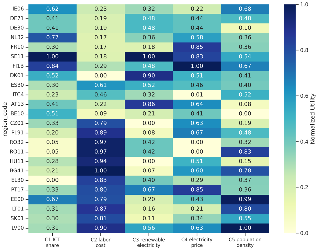
The normalized decision matrix confirms that no single regional group dominates all five criteria at the same time (Figure 2). The strongest overall profile is concentrated in the Nordic–Baltic part of the sample, but this advantage is internally differentiated rather than uniform. SE11 combines the highest normalized values for ICT specialist share and renewable electricity. LV00 combines the lowest territorial pressure in the sample with low labor cost and a moderate electricity price. EE00 shows a similarly sparse footprint, with cheap labor but a more mid-range electricity cost and a low renewable share, so its favorable profile is driven primarily by density and workforce conditions rather than by energy. FI1B also remains consistently strong, supported by a balanced combination of talent, electricity price and moderate territorial pressure.

At the same time, the mature Western and FLAP-D markets do not dominate the matrix across all criteria. Their main structural weakness is labor cost, and in some cases territorial pressure. IE06, NL32, FR10, DE71 and DE30 all record C2_norm values at or below 0.24, which places them close to the expensive end of the sample. DE30 is the clearest example of this trade-off: it combines a strong ICT base with very high density, reaching 4320.5 persons/km² in raw terms and only 0.10 after normalization on the transformed C5 scale. NL32 shows a similar tension, with strong talent performance but relatively weak positions on labor cost and density. The most pronounced criterion-level contrast concerns labor cost and territorial pressure, where the FLAP-D group occupies the unfavorable tail of the distribution: DE30 records the third-highest density in the sample at 4320.5 persons/km², behind BE10 (7660.0) and AT13 (4941.5), and the FLAP-D nodes represented in the sample (IE06, DE71, NL32, FR10) carry labor costs ranging from EUR 38.0/h (IE06) to EUR 40.4/h (FR10).

The low-density advantage also needs to be read carefully. EE00 and LV00 are genuinely sparse regions at 31.3 and 29.7 persons/km² respectively, and therefore occupy the favorable extreme of the density criterion. SE11, by contrast, is not low-density in absolute terms. Its raw value is 372.1 persons/km², and its normalized utility on C5 is 0.54, which places it in the middle of the distribution rather than at the best end. Its strength comes from the combination of very strong C1 and C3 values, not from exceptionally low territorial pressure.

Two other profiles stand out in the normalized matrix. PT17 combines low labor cost, low electricity price and high renewable electricity share, which makes it unusually well balanced across cost and sustainability criteria. BG41 performs strongly on labor cost and density and therefore enters the upper part of the ranking despite a much weaker renewable electricity profile than the leading Nordic cases.

4.2. Deterministic Rankings and Inter-Engine Agreement

The deterministic block shows that the three MCDA engines tell a broadly similar story, but not with identical strength in every scenario.

Table 2. Spearman rank correlations across deterministic engines.

Scenario	ρ (WSM, TOPSIS)	ρ (WSM, VIKOR)	ρ (TOPSIS, VIKOR)
Balanced	0.903	0.811	0.630
CostPressure	0.907	0.910	0.846
GreenFirst	0.877	0.881	0.984
TalentFirst	0.949	0.856	0.825

reports the Spearman correlations across WSM, TOPSIS and VIKOR. Agreement is high overall, with all WSM-TOPSIS and WSM-VIKOR correlations above 0.80. The lowest inter-engine agreement appears between TOPSIS and VIKOR under the Balanced scenario (ρ = 0.630), while the same pair converges almost perfectly under GreenFirst (ρ = 0.984). This means that aggregation logic matters most when no criterion block dominates the weights and matters less when renewable electricity clearly leads the profile.

The weaker TOPSIS-VIKOR agreement under the Balanced scenario can be explained by the different logic of the two methods. TOPSIS rewards proximity to an ideal profile and can favor regions with very strong values on one or more criteria, even when some weaknesses remain. VIKOR follows a compromise-ranking logic and gives more weight to balanced profiles with lower regret across criteria. This is why LV00 performs especially well under VIKOR in the Balanced scenario: it combines very low density with favorable cost conditions and has no severe penalty on the main cost-side criteria. SE11 remains stronger under TOPSIS because its high ICT specialist share and renewable electricity profile place it closer to the ideal solution.

The WSM ranks in

Table 3. Condensed deterministic ranks for the 24 selected NUTS-2 regions. Lower rank values indicate more favorable positions within the corresponding method and weighting scenario.

NUTS-2 Code	Region Name	Country	Country Code	WSM Balanced	WSM CostPressure	WSM GreenFirst	WSM TalentFirst	TOPSIS Balanced	VIKOR Balanced
AT13	Wien	Austria	AT	13	16	6	14	6	15
BE10	Région de Bruxelles-Capitale	Belgium	BE	24	24	24	24	24	24
BG41	Yugozapaden	Bulgaria	BG	6	4	11	7	8	11
CZ01	Praha	Czechia	CZ	17	8	21	15	18	19
DE30	Berlin	Germany	DE	22	22	13	20	21	16
DE71	Darmstadt	Germany	DE	16	20	10	18	20	10
DK01	Hovedstaden	Denmark	DK	8	19	5	10	7	17
EE00	Eesti	Estonia	EE	4	6	7	3	5	5
EL30	Attiki	Greece	EL	18	15	14	21	14	20
ES30	Comunidad de Madrid	Spain	ES	10	11	8	11	10	6
FI1B	Helsinki-Uusimaa	Finland	FI	3	3	4	2	4	3
FR10	Île-de-France	France	FR	20	14	19	22	22	12
HU11	Budapest	Hungary	HU	19	9	22	16	17	21
IE06	Eastern and Midland	Ireland	IE	15	21	16	9	19	7
ITC4	Lombardia	Italy	IT	23	23	23	23	23	23
LT01	Sostinės regionas	Lithuania	LT	7	10	17	8	11	8
LV00	Latvija	Latvia	LV	2	1	3	4	2	1
NL32	Noord-Holland	Netherlands	NL	12	17	9	6	15	9
PL91	Warszawski stołeczny	Poland	PL	9	7	15	12	12	13
PT17	Área Metropolitana de Lisboa	Portugal	PT	5	2	2	5	3	2
RO11	Nord-Vest	Romania	RO	11	13	12	17	9	18
RO32	Bucureşti-Ilfov	Romania	RO	21	18	18	19	13	22
SE11	Stockholm	Sweden	SE	1	5	1	1	1	4
SK01	Bratislavský kraj	Slovakia	SK	14	12	20	13	16	14

show that SE11 leads three of the four deterministic scenarios, ranking first under Balanced, GreenFirst and TalentFirst. LV00 takes first place under CostPressure, which is consistent with its very favorable combination of low labor cost, low electricity price and very low density. FI1B remains in the top four in every scenario, while PT17 stays in the top five throughout. At the bottom end, BE10 ranks last in all four WSM scenarios and ITC4 ranks 23rd in all four, which indicates a persistent structural disadvantage rather than scenario-specific weakness. A small but useful nuance appears under VIKOR in the Balanced scenario, where LV00 takes first place rather than SE11, which suggests that the compromise-ranking logic rewards LV00’s combination of very low density and favorable cost conditions more strongly than the talent-and-renewables advantage of SE11.

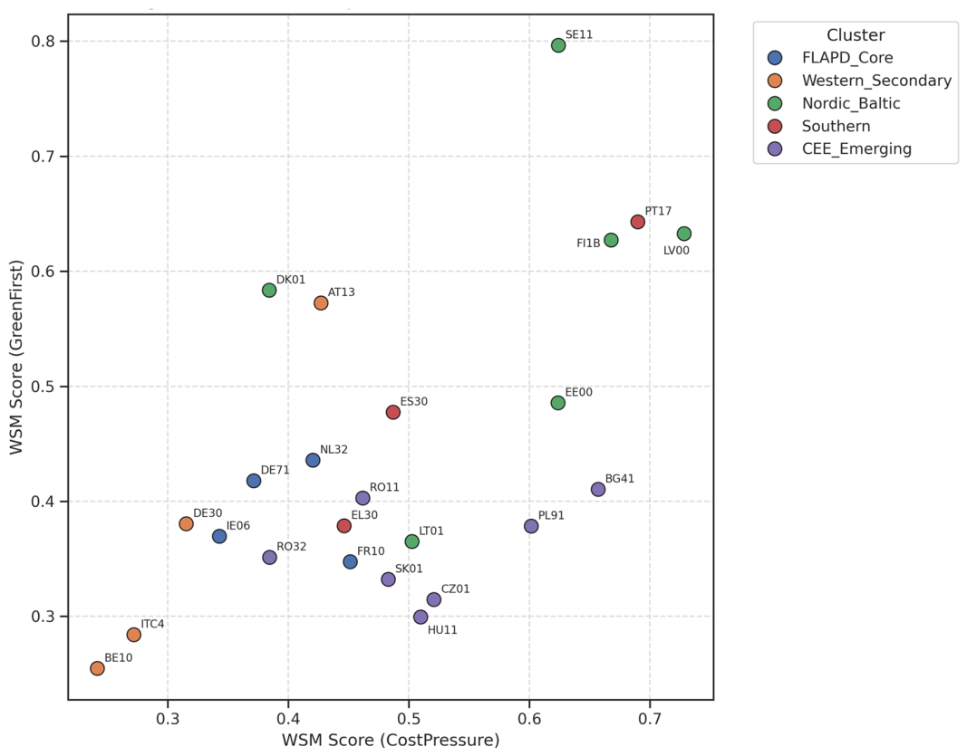
The scenario dependence of a few mid-ranked regions is also important. DK01 moves from eighth in Balanced to 19th in CostPressure, then back to fifth in GreenFirst. NL32 improves from 12th in Balanced to sixth in TalentFirst but falls to 17th in CostPressure. AT13 rises to sixth in GreenFirst but remains 13th–16th elsewhere. These movements are consistent with the figure logic: regions that combine strong talent or renewable profiles with expensive labor become highly sensitive to the weight placed on cost criteria. Figure 3 visualizes this scenario dependence by comparing WSM scores under the CostPressure and GreenFirst scenarios.

4.3. Global Stochastic Rank Behavior

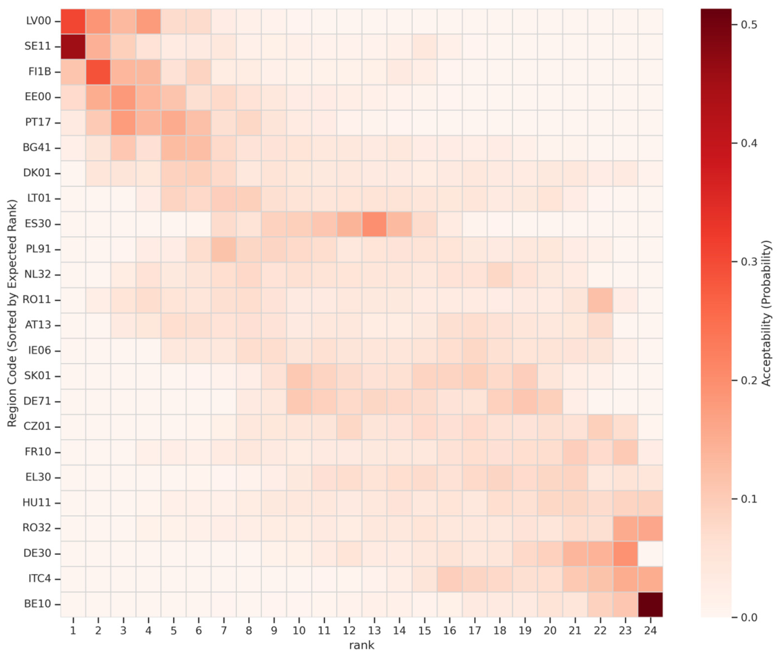
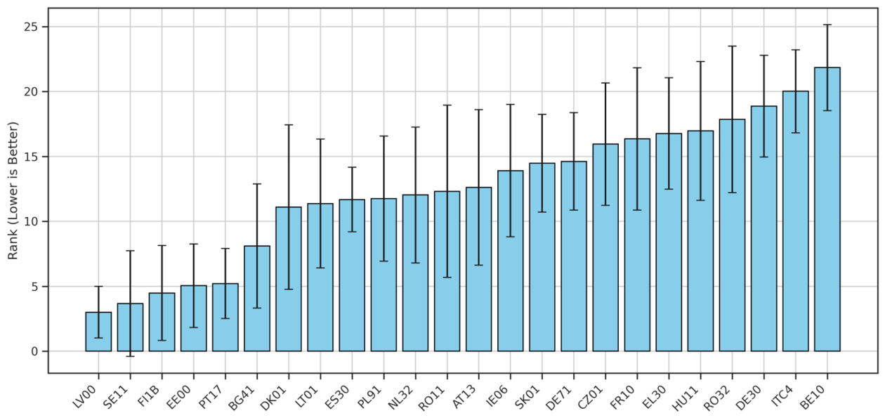
The global stochastic audit sharpens the deterministic picture by exploring the full weight simplex rather than four named scenarios. Figure 4 shows the full 24 × 24 rank acceptability matrix, with rows sorted by expected rank. The upper part of the matrix is dominated by a narrow Nordic–Baltic group. LV00 records an expected rank of 3.01 with SD = 1.99, SE11 an expected rank of 3.67 with SD = 4.07, FI1B 4.49 with SD = 3.66, and EE00 5.05 with SD = 3.21. PT17 follows closely with an expected rank of 5.22 and SD = 2.69. These are the only regions that combine clearly favorable average positions with non-trivial top-3 acceptability.

The same pattern appears in the top-rank probabilities. SE11 has the highest top-1 acceptability in the sample at 0.455 and the highest top-3 acceptability at 0.695. LV00 follows with b1 = 0.306 and top-3 acceptability = 0.624. FI1B and EE00 remain clearly competitive with top-3 probabilities of 0.537 and 0.406, while PT17 reaches 0.317. These values show that the leading group is not defined only by good average ranks. It also occupies a large portion of the admissible weight space.

The lower part of the expected-rank ordering is equally clear in

Table 4. Random-weighting audit summary. DRI is reported as an auxiliary baseline-alignment indicator, together with expected rank, rank standard deviation, rank acceptability.

Region	Cluster	E[r]	SD[r]	b1	Top-3	DRI
LV00	Nordic_Baltic	3.007	1.989	0.306	0.624	0.930
SE11	Nordic_Baltic	3.673	4.066	0.455	0.695	0.884
FI1B	Nordic_Baltic	4.487	3.661	0.112	0.537	0.891
EE00	Nordic_Baltic	5.052	3.214	0.073	0.406	0.893
PT17	Southern	5.215	2.690	0.036	0.317	0.908
BG41	CEE_Emerging	8.104	4.774	0.019	0.176	0.833
DK01	Nordic_Baltic	11.096	6.332	0.000	0.096	0.758
LT01	Nordic_Baltic	11.374	4.960	0.000	0.002	0.781
ES30	Southern	11.678	2.487	0.000	0.000	0.889
PL91	CEE_Emerging	11.757	4.817	0.000	0.003	0.813
NL32	FLAPD_Core	12.035	5.230	0.000	0.029	0.802
RO11	CEE_Emerging	12.312	6.631	0.000	0.075	0.747
AT13	Western_Secondary	12.616	5.990	0.000	0.037	0.767
IE06	FLAPD_Core	13.909	5.090	0.000	0.000	0.807
SK01	CEE_Emerging	14.475	3.762	0.000	0.000	0.857
DE71	FLAPD_Core	14.616	3.756	0.000	0.000	0.849
CZ01	CEE_Emerging	15.945	4.707	0.000	0.000	0.823
FR10	FLAPD_Core	16.348	5.474	0.000	0.000	0.784
EL30	Southern	16.767	4.289	0.000	0.000	0.840
HU11	CEE_Emerging	16.963	5.347	0.000	0.001	0.802
RO32	CEE_Emerging	17.856	5.635	0.000	0.001	0.790
DE30	Western_Secondary	18.867	3.921	0.000	0.000	0.847
ITC4	Western_Secondary	20.013	3.201	0.000	0.000	0.857
BE10	Western_Secondary	21.836	3.316	0.000	0.000	0.906

. DE30 falls to an expected rank of 18.87, ITC4 to 20.01 and BE10 to 21.84. In these cases, the weak positions are not isolated scenario effects. They persist across a broad range of weight vectors. At the same time, the most interesting part of Figure 4 is the middle rather than the bottom: regions such as DK01, NL32, PL91, AT13 and RO11 show a much wider distribution of acceptable rank positions, which signals a stronger dependence on the exact preference structure than the headline ranks alone would suggest.

4.4. Expected Rank, Dispersion and the Distinction Between Performance and Stability

Figure 5 clarifies the difference between performance and stability. LV00 combines the best expected rank, E[r] = 3.01, with the lowest rank standard deviation, SD = 1.99. PT17 ranks slightly lower on average, E[r] = 5.22, but remains more stable than most regions around it, with SD = 2.69. FI1B and EE00 also remain in the favorable zone, although with wider dispersion than LV00.

The middle of the ranking is where the distinction becomes analytically important. ES30 has an expected rank of 11.68 but a much lower SD than most of its neighbors in the table, only 2.49, which suggests a stable middle-tier position. DK01 reaches a similar average position, E[r] = 11.10, but with SD = 6.33, the second-highest value in the entire sample. Its profile explains why. DK01 has a very strong renewable electricity score and a reasonable density position, but it also has the highest labor cost in the sample, EUR 47.1/h. As soon as labor cost receives greater emphasis, its position deteriorates sharply. In other words, DK01 is not mediocre. It is highly conditional.

The most volatile regions are RO11, DK01 and AT13, with SD values of 6.63, 6.33 and 5.99 respectively. All three combine at least one strong criterion with at least one strong penalty, which makes them highly sensitive to the weight structure. At the other end, the three most stable regions by rank dispersion are LV00, ES30 and PT17. Stability, however, should not be confused with attractiveness. BE10 is a good counterexample. Its SD is only 3.32 and its DRI is high, but this reflects stable weakness rather than stable strength: it remains near the bottom across almost the entire weight simplex.

4.5. Scenario Trade-Offs and the Interpretation of DRI

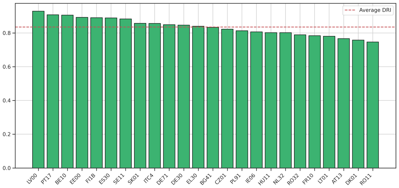
The DRI summary in Figure 6 should be read as an indicator of alignment with the Balanced baseline, not as a substitute for attractiveness. The highest DRI values are recorded by LV00 (0.930), PT17 (0.908), BE10 (0.906), EE00 (0.893) and FI1B (0.891). The interpretation differs sharply across these cases. For LV00, PT17, EE00 and FI1B, a high DRI reflects rank stability around a good or very good baseline position. For BE10, the same pattern reflects stable underperformance. It ranks last in the deterministic WSM baseline and remains close to the bottom under stochastic perturbation, which yields a high DRI without implying that it is an attractive location.

The lowest DRI values identify the regions whose stochastic positions diverge most strongly from their Balanced-scenario baseline. RO11 has the lowest DRI in the sample at 0.747, followed by DK01 at 0.758 and AT13 at 0.767. These are exactly the regions that also show the widest dispersion in Figure 5. In practical terms, they are the cases where a single deterministic rank is most likely to mislead if it is interpreted without uncertainty analysis.

Figure 6 therefore adds a useful summary layer, but only when read together with expected rank and rank standard deviation. A high DRI attached to a strong expected rank is a sign of dependable attractiveness. A high DRI attached to a poor expected rank is a sign of persistent weakness. A low DRI indicates that the deterministic baseline does not adequately summarize the region’s broader rank behavior under weight uncertainty.

4.6. Local Stability near the Balanced Profile

The local Dirichlet sensitivity analysis (

Table 5. Local Dirichlet sensitivity results.

Region	E[r] κ = 20	E[r] κ = 50	E[r] κ = 100	SD[r] κ = 20	SD[r] κ = 50	SD[r] κ = 100
AT13	12.494	12.527	12.159	4.793	3.876	3.196
BE10	23.401	23.834	23.933	1.285	0.554	0.319
BG41	6.808	6.307	6.221	2.545	1.332	0.826
CZ01	16.424	16.722	16.855	3.662	2.685	2.067
DE30	20.509	21.482	21.703	2.633	1.631	1.220
DE71	15.690	16.375	16.427	3.058	2.368	2.033
DK01	10.286	9.835	9.169	4.709	3.606	2.869
EE00	4.091	3.993	4.128	1.549	1.053	0.812
EL30	17.485	17.657	18.041	3.070	2.450	2.005
ES30	10.759	10.332	10.139	1.715	1.267	1.016
FI1B	3.310	3.147	2.990	1.806	1.111	0.819
FR10	17.448	18.491	18.704	4.040	2.897	2.391
HU11	17.782	18.236	18.564	3.962	2.931	2.229
IE06	14.409	14.658	14.738	3.985	3.262	2.506
ITC4	21.757	22.317	22.651	1.949	1.174	0.721
LT01	10.360	9.362	9.096	3.306	2.300	2.046
LV00	2.265	1.977	1.996	1.156	0.911	0.757
NL32	11.681	11.615	11.245	4.001	3.259	2.603
PL91	10.700	10.059	9.819	3.241	2.500	2.230
PT17	4.492	4.528	4.582	1.470	0.941	0.661
RO11	12.009	11.198	11.159	4.937	3.741	3.107
RO32	19.305	19.733	20.253	3.815	2.846	2.024
SE11	2.147	1.648	1.365	2.009	1.076	0.682
SK01	14.386	13.964	14.062	2.853	2.265	1.896

) confirms that the upper part of the ranking is not an artifact of one arbitrary concentration parameter. Across κ = 20, 50 and 100, the same leading group remains in place. SE11 moves from E[r] = 2.15 to 1.65 and then 1.37 as the distribution becomes more concentrated around the Balanced vector. LV00 remains near rank 2 throughout, with expected ranks of 2.27, 1.98 and 2.00. FI1B stays close to rank 3, while EE00 and PT17 remain near ranks 4 and 5. This pattern is consistent with regions whose performance is already strong under the Balanced deterministic baseline and remains stable under local perturbation around that profile.

The same analysis also identifies regions that remain fragile even when the exploration is restricted to a neighborhood of the Balanced vector. At κ = 20, the highest local rank dispersion belongs to RO11 (SD = 4.94), AT13 (SD = 4.79) and DK01 (SD = 4.71). Even when κ rises to 100, all three still show comparatively large local SD values: 3.11 for RO11, 3.20 for AT13 and 2.87 for DK01. This means that their instability is not only a property of the full simplex. It also remains visible under moderate local weight perturbations.

The local results are therefore consistent with the global audit. The leading Nordic–Baltic set remains stable both globally and locally. PT17 also retains a strong and stable profile near the Balanced center. By contrast, regions such as DK01 and RO11 remain structurally sensitive whether the analyst explores the entire weight space or only a balanced neighborhood around the consensus profile.

5. Discussion

5.1. Performance, Stability and Regional Differentiation

The results point to a clear distinction between regional performance and regional stability. The leading positions are not occupied by the established Western metropolitan markets, but by a narrower Nordic–Baltic set in which good average performance is combined with stronger behavior under weight uncertainty. LV00 is the clearest case, because it combines the best expected rank with the lowest global rank dispersion in the sample. SE11, FI1B and EE00 also remain in the leading group, while PT17 emerges as the strongest Southern case because it combines a good expected rank with comparatively low dispersion. This means that the upper part of the ranking is not only a deterministic outcome driven by one scenario. It also persists when the weight structure is allowed to vary broadly.

At the same time, the results do not support a simple mature-versus-emerging dichotomy. The FLAP-D and Western metropolitan regions retain clear advantages in ICT workforce depth, but in this study those advantages are offset by higher labor costs and, in several cases, stronger territorial pressure. This is visible not only in the normalized profiles but also in the scenario results. NL32 is a useful example: it remains strong on ICT depth, yet its position deteriorates when labor cost becomes more important. DK01 shows a different kind of tension. It performs well when renewable electricity is emphasized, but it becomes highly unstable once labor cost receives greater weight. These cases matter because they show that a region can look attractive in a static ranking while remaining highly conditional in a broader decision space.

A second message concerns the value of the stochastic layer itself. The deterministic block already showed high agreement across WSM, TOPSIS and VIKOR, which means the rankings are not driven by one arbitrary aggregation engine. However, that agreement does not eliminate uncertainty about preference structure. The global stochastic audit adds exactly that missing layer. It distinguishes regions that remain competitive across a large part of the feasible weight space from regions whose good positions depend on a much narrower combination of priorities. This is the practical meaning of rank acceptability in the present study. A region that reaches the first place only under one narrow weighting profile is analytically different from a region that remains near the top across many admissible profiles, even if their best deterministic ranks look similar at first sight. This is the main contribution of the random-weighting component of the workflow.

5.2. What Stochastic Robustness Adds to Deterministic Ranking

Seen in this light, the paper does more than reorder 24 regions. It shows why a one-shot ranking can be incomplete for infrastructure planning. The deterministic scenarios answer the question, “who performs well under a named priority profile?” The stochastic layer answers a different question, namely, “who remains competitive when the priority profile itself is uncertain?” This distinction is methodologically important because early-stage infrastructure decisions rarely begin with stable and fully agreed stakeholder weights. In that context, expected rank, rank dispersion and top-rank acceptability add information that fixed scenarios cannot provide. They are the quantities that separate dependable candidates from scenario-dependent ones. This is precisely what the rank acceptability results capture: the share of admissible weight draws under which a region reaches a given rank.

The DRI adds a useful but secondary perspective. It indicates alignment with the Balanced baseline rather than attractiveness itself. BE10 is the clearest example: its DRI is high because it remains close to its Balanced position, but that position is near the bottom of the ranking. The index therefore captures stability of rank behavior, not desirability in substantive terms. It is most informative when considered together with expected rank and rank standard deviation.

The local Dirichlet analysis strengthens this argument because it shows that the upper part of the ranking is not an artifact of one arbitrary concentration parameter around the Balanced profile. The same leading group remains in place across κ = 20, 50 and 100, while the same fragile cases continue to show comparatively high local dispersion. This is important because it shows that the results are not sensitive only at the global simplex level. They also remain structured in a narrower neighborhood around a plausible consensus profile. In practical terms, the leading set is globally competitive and locally stable, while the fragile set remains fragile under both broad and narrow preference perturbations.

5.3. Implications for Spatial Decision Support

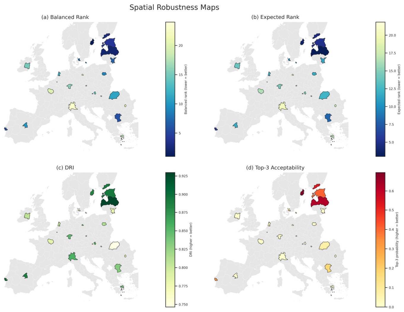
The spatial maps are where this distinction becomes easiest to interpret. Figure 7 is an important visualization in the paper because it brings the four analytical layers together in a single spatial frame: deterministic Balanced rank, global expected rank, DRI and top-3 acceptability. Read together, the four panels show that a northern high-performing pattern remains visible across the rank-based metrics, while the DRI panel adds a more nuanced view of stability. The pattern is not identical in every panel, but it is consistent enough to show that the main finding is not an artifact of any single indicator. Regions in the Nordic–Baltic zone remain prominent not only in deterministic performance, but also in stochastic expected rank and in the probability of remaining in the top group. This aligns directly with the spatial robustness perspective adopted in this study. At the planning level, this pattern suggests that the Nordic–Baltic set represented by SE11, LV00, FI1B, EE00 is a plausible first-stage corridor for geo-distributed infrastructure screening, while PT17 represents a Southern case where grid access, renewable-energy integration and local ICT conditions deserve closer project-level assessment.

Figure 7d adds a more specific spatial message. The top-3 acceptability surface is not diffuse across Europe. It is concentrated in a visible northern belt centered on SE11, LV00 and EE00, with FI1B extending that high-acceptability northern pattern and PT17 standing out as a separate Southern exception rather than as part of the same corridor. In descriptive terms, the regions most often appearing in the top three form a visible high-acceptability pattern rather than a diffuse distribution. This should be read as a descriptive spatial pattern rather than as evidence of statistically tested spatial autocorrelation. But it does show that once weight uncertainty is taken seriously, the geography of robust attractiveness becomes more concentrated than the deterministic tables alone might suggest.

From a decision-support perspective, this matters because the paper is positioned at a macro-regional feasibility level. It is not a parcel-level engineering tool. Within that scope, the maps are not decorative end products. They are the interface through which the core analytical distinction becomes visible at regional scale. The study therefore speaks to the spatial MCDA and spatial decision support agenda in a concrete way: it shows how open regional data, multi-engine validation and stochastic rank analysis can be combined into a reproducible regional screening framework whose outputs remain interpretable geographically.

5.4. Limitations and Scope Boundaries

This study has several limitations that should frame the interpretation of the results. First, four of the five criteria (C1–C4) rely on national-level values assigned to the selected NUTS-2 regions. Because these indicators are intensive variables, this choice does not inflate totals or create artificial size effects across regions. Even so, it suppresses intra-country variation for those criteria. The comparison is therefore stronger as a cross-country and cross-cluster regional screening exercise than as a tool for fine within-country discrimination. For non-euro countries, labor cost values expressed in euros may reflect exchange rate effects in addition to structural differences in regional labor markets.

Second, the study is deliberately macro-regional in scope. It does not include parcel-level or engineering variables such as fiber routes, latency, substation constraints, cooling climate, land availability, seismic exposure or local permitting conditions. For that reason, the framework should be read as a first-stage regional screening tool, not as a substitute for site-specific engineering due diligence.

A related limitation concerns the interpretation of population density. In this study, lower density reduces the territorial-pressure score in the screening model, but it does not imply easier local siting. Less dense regions may still face constraints linked to land ownership, agricultural land conversion, landscape impact, biodiversity, local opposition or permitting. These issues are outside the Eurostat-based macro-regional matrix and require site-level assessment.

Third, the analysis is cross-sectional and anchored in the 2022 reference matrix. This was the most recent year for which the five-criterion matrix could be assembled with complete coverage and consistent filters across the selected regions, although the upstream extraction workflow is designed to scan the Eurostat series from 2014 onward and can produce a validated matrix for years in which all five criteria pass the applied completeness audit. The results therefore partly reflect the particular energy and cost environment of 2022, and a temporal extension would be the most direct next step if the framework is to move from structural comparison toward a broader assessment of resilience over time.

Fourth, the spatial interpretation remains descriptive rather than inferential. Because the 24 regions were selected purposively and are geographically discontinuous, formal spatial autocorrelation tests such as Moran’s I were not applied. The northern concentration visible in Figure 7d should therefore be read as a descriptive spatial pattern rather than as a statistically tested autocorrelation result.

Finally, DRI is a study-specific derived indicator. It is useful as a compact summary of how closely stochastic rank behavior remains aligned with the Balanced baseline, but it should be read together with expected rank and rank dispersion rather than as a standalone quality score.

5.5. A Three-Part Typology of Regional Attractiveness

Taken together, the findings suggest that regional attractiveness for geo-distributed data center development should not be read as a simple distinction between high and low ranks. The more useful distinction is between stable strong profiles, stable weak profiles and condition-dependent profiles.

The stable strong group includes LV00, SE11, FI1B, EE00 and PT17. These regions do not share exactly the same profile, but they combine enough advantages to remain competitive across weight structures. Their common drivers are combinations of low or moderate labor cost, lower territorial pressure or manageable density and in several cases, a medium-to-high renewable electricity position. SE11 is the main exception on density, because its strength comes more from ICT workforce depth and renewable electricity than from a low-density profile.

The stable weak group is represented most clearly by BE10 and ITC4. These regions remain close to the bottom across scenarios and stochastic draws. Their weak positions are linked mainly to high labor cost, high territorial pressure or an unfavorable combination of both. In these cases, stability does not indicate attractiveness. It indicates persistent disadvantage under the selected criteria.

The condition-dependent group includes DK01, AT13, NL32 and RO11. These regions have at least one strong criterion, such as renewable electricity, ICT workforce depth or density, but also one or more clear penalties. Their rank positions therefore depend more strongly on the weighting profile. This group is important for decision support because it shows where a single deterministic rank can hide substantial sensitivity to decision priorities.

6. Conclusions

This study developed a reproducible spatial decision support framework for comparing macro-regional attractiveness and rank stability across 24 selected European NUTS-2 regions. The framework combines a Eurostat-based 2022 decision matrix, deterministic MCDA comparison, a random-weighting audit based on SMAA principles and local Dirichlet sensitivity around a neutral baseline.

The results show that the most stable high-performing profiles are concentrated in a small set of regions rather than in the established FLAP-D market reference alone. LV00, SE11, FI1B, EE00 and PT17 form the main high-performing group across the stochastic rank metrics, although their advantages are not identical. LV00 and PT17 benefit from favorable cost and territorial-pressure conditions, SE11 is stronger through ICT workforce depth and renewable electricity, while FI1B and EE00 remain competitive through more balanced combinations of criteria.

Methodologically, the study shows why deterministic rankings should be complemented by weight-uncertainty analysis in early-stage infrastructure screening. The deterministic block checks whether WSM, TOPSIS and VIKOR tell broadly similar stories under named priority profiles. The stochastic and local Dirichlet layers then separate stable strong profiles, stable weak profiles and condition-dependent profiles. In this structure, DRI is useful as a secondary baseline-alignment indicator, but expected rank, rank dispersion and rank acceptability remain the main evidence for robustness.

The spatial contribution comes from placing these rank-based measures back onto the NUTS-2 geography. The maps show that robust attractiveness has a visible Nordic–Baltic concentration, with PT17 as a separate Southern case. This supports the paper’s framing as a spatial decision support study rather than a purely tabular MCDA ranking exercise.

The framework is designed for first-stage macro-regional screening. Because C1–C4 rely on national intensive proxies assigned to selected NUTS-2 regions, the analysis is stronger for cross-country and selected-region comparison than for fine within-country discrimination. Future work can extend the same logic by rebuilding validated matrices for other years, incorporating compatible sub-national data where available and linking the macro-regional layer to finer engineering variables such as local grid constraints, land conditions or cooling-related climate factors.