ICDL-Agent: A Tool-Augmented LLM Agent for Automatic Instrument Workflows in Incoherent Doppler LiDAR Analysis

Abstract

Large language models (LLMs) offer new possibilities for natural-language interaction with geospatial analysis systems, but their use in remote sensing instrument data analysis remains limited by weak execution control, poor reproducibility, and limited integration with domain-specific computation. The paper presents an agent for Incoherent Doppler wind LiDAR (ICDL) data analysis, named ICDL-Agent, a tool-augmented LLM framework for remote sensing instrument workflows. The system maps conversational user requests to executable analysis pipelines for wind retrieval, uncertainty estimation, visualization, and higher-level diagnostics through structured planning over a registry of domain-specific tools. To improve execution reliability, the system combines schema-constrained workflow generation, shared-state reuse of intermediate scientific products, and validation with bounded repair. In addition to supporting routine LiDAR processing, the framework can generate new tools when required and adapt to related analytical tasks through domain-aware guidance and procedural documentation. We evaluate the system on multiple atmospheric wind-observation datasets in China and show that it faithfully reproduces the refined Doppler wind-retrieval pipeline, achieving representative R²/MAE values of 0.52/3.73 m/s against ERA5 and 0.80/2.31 m/s against radiosonde observations, while supporting downstream analyses such as profile comparison, climatological interpretation, and gravity-wave diagnostics. More broadly, this study demonstrates how constrained LLM orchestration can support LiDAR researchers, remote-sensing instrument teams, and geospatial analysts seeking transparent, reproducible, and automated scientific data-processing workflows.

1. Introduction

Atmospheric wind observations are an important source of geospatial environmental information for studying dynamic atmospheric transport processes, wave activity, and circulation structure across the troposphere and middle atmosphere. Among the available observing techniques, Light Detection and Ranging (LiDAR) equipment provides high-resolution wind measurements with strong value for environmental monitoring and atmospheric analysis [1,2,3,4,5,6]. Previous Incoherent Doppler LiDAR (ICDL) studies established the capability of middle-atmosphere density [2,7], temperature [2,6,8,9], and wave observations [2,7,10,11], while early Fabry-Pérot-interferometer (FPI)-based studies [1,3,4,5] provided the theoretical basis for Doppler frequency discrimination and wind retrieval [1,3,4,5,6,8,9,12,13]. However, the practical use of these observations still depends on complex, instrument-specific processing chains [7,8,9,10,11,12,13] including wind retrieval [1,3,4,5,6,8,9,12,13], FPI analysis [12], comparison with satellite wind observations [10], gravity-wave characterization [7,11], zero-Doppler correction [13], and so on. In many research settings, these stages remain implemented as loosely connected scripts that are difficult to reuse, extend, or adapt across datasets, observing campaigns, instruments, and analytical objectives. As a result, geospatial environmental observations produced by ICDL remain scientifically valuable, but the corresponding instrument-specific analysis workflows are still difficult to adapt, reuse, and reproduce.

Large language models (LLMs) offer a possible route toward more accessible analysis because they can interpret natural-language instructions, plan multi-step actions, and generate executable code [14,15,16,17,18,19,20,21,22]. Transformer-based language modeling provides the architectural basis for modern LLMs [14], while large-scale few-shot learning demonstrates its ability to generalize from limited examples [15]. Related studies further show that prompting can function as a form of programmable control [16], that LLMs can interact with embodied or software environments [17], that they can also learn to use external tools [18], and that reasoning-action prompting can combine intermediate reasoning with executable actions [21].

More recently, agentic LLM systems have shown strong capabilities in tool use, workflow orchestration, external software interaction, and multi-agent coordination. In parallel, recent studies have begun to explore the use of LLMs for geospatial data processing and workflow automation, indicating broader potential for tool-guided analytical systems in this field [23,24]. Recent multimodal remote sensing large models, such as SkyEyeGPT [25], have further shown that instruction-tuned vision-language models can support image captioning, visual grounding, visual question answering, referring expression generation, and scene classification for remote sensing imagery. However, most existing systems are designed either for a more generalized context or for specialized applications in other domains [26,27,28,29,30,31]. Meanwhile, artificial intelligence has also been increasingly integrated into wind LiDAR retrieval, for example, through deep-learning-based wind reconstruction [32,33,34,35]. Yet these developments have so far focused on specific retrieval components or tasks. To our knowledge, a constrained agent framework dedicated specifically to end-to-end wind LiDAR analysis has not yet been established. Scientific instrument analysis imposes a different set of requirements, including numerical reproducibility, physically consistent outputs, a structured intermediate state, and explicit analytical provenance. Flexible language generation alone is therefore insufficient. The central challenge is not simply how to apply an LLM to LiDAR analysis, but how to embed it within a constrained execution framework that can orchestrate trusted tools, preserve intermediate computational products, and recover from failure without compromising scientific traceability.

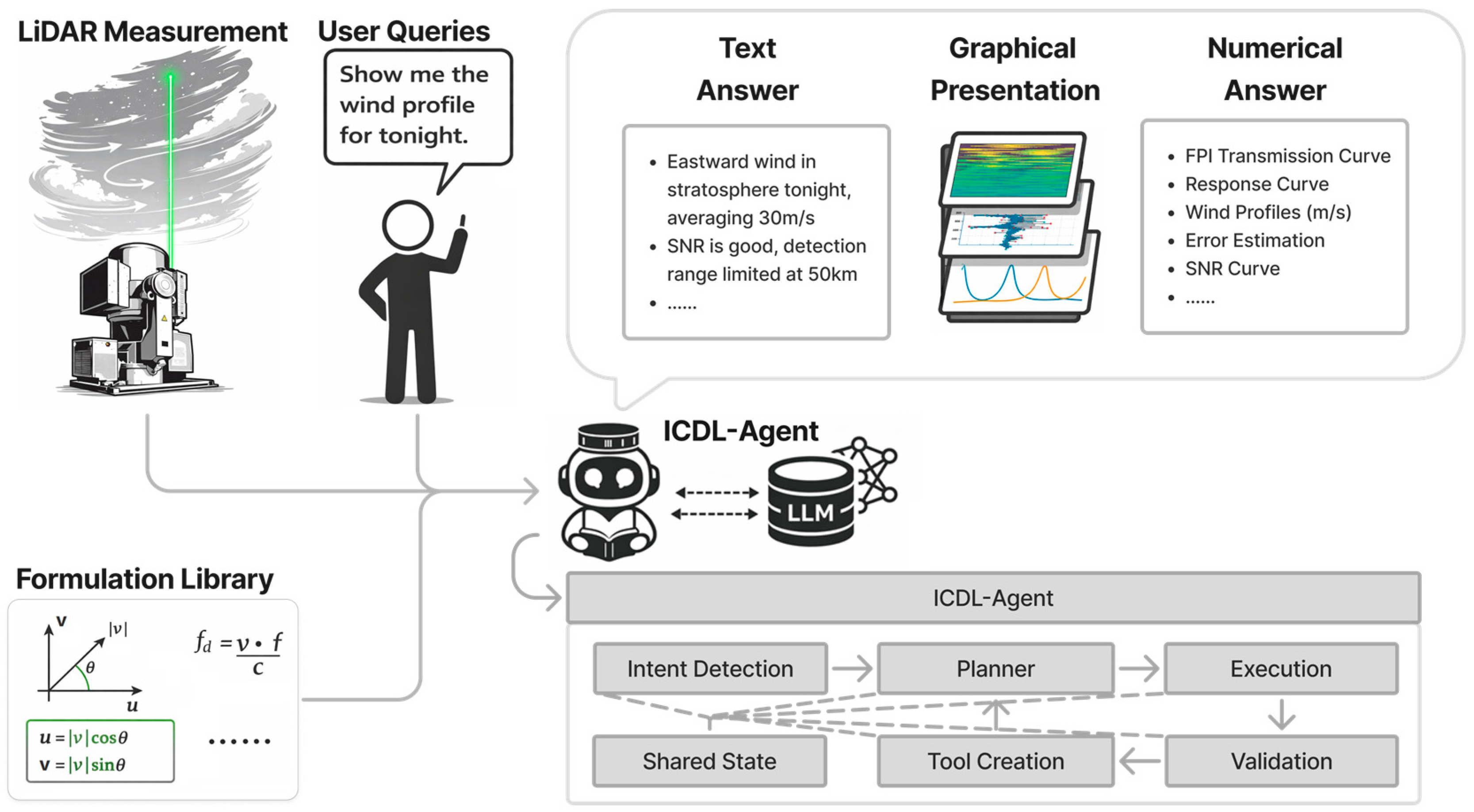
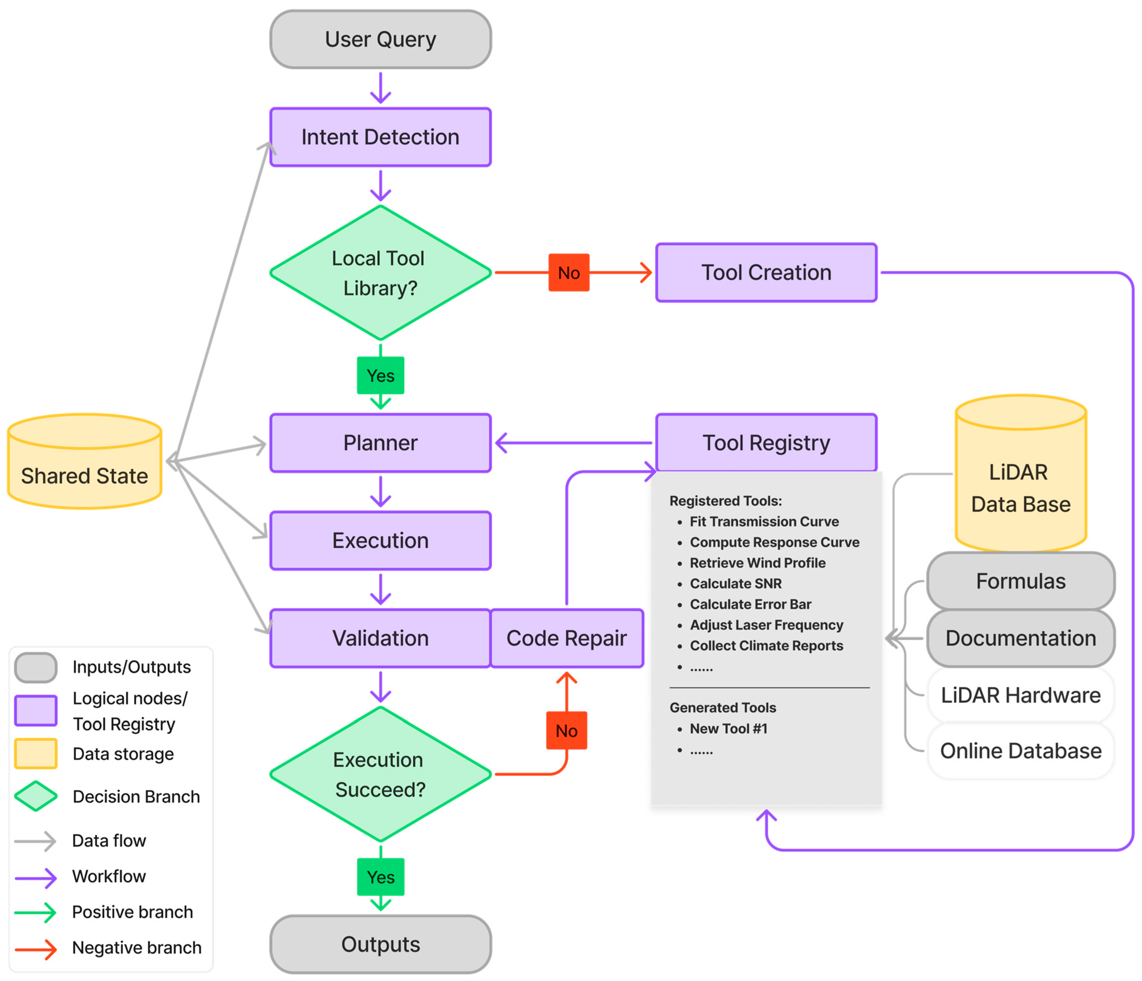
The paper presents ICDL-Agent, an LLM-driven, tool-augmented agent for autonomous processing of Incoherent Doppler wind LiDAR data, illustrated in Figure 1. The agent consumes conversational task descriptions, domain formulas, related documentation, and raw datasets, and carries out intent detection, schema-constrained planning, tool execution, validation, and, when necessary, tool generation and repair. The tool library can evolve to incorporate new functionalities, allowing the same architecture to support new user queries and operate across different LiDAR systems and data formats. Users interact with the system exclusively through natural-language queries, which are resolved using both conversational context and previously computed scientific artifacts. Unlike generic conversational memory, the shared state stores physically meaningful intermediate products that can be reused, refined, and inspected across turns without rerunning the entire workflow from scratch. The illustration of the agent system is shown in Figure 1.

Applied to multiple Rayleigh Doppler wind LiDAR datasets from atmospheric research in China, the agent reproduces and improves the traditional hand-coded pipelines for wind profile retrieval and derived diagnostics while substantially reducing the amount of instrument-specific code that must be developed and maintained. At the same time, every processing step remains explicit and inspectable as human-readable code, tool calls, and intermediate computational artifacts, preserving transparency and scientific reproducibility. Although we focus on Doppler wind LiDAR, the approach can generalize to other complex instruments in which analysis consists of modular numerical procedures that can be exposed as tools and orchestrated by an LLM-based agent.

This study is guided by three research questions: (1) Can a tool-augmented LLM agent reliably orchestrate the main computational stages of ICDL wind retrieval and visualization through natural-language interaction? (2) Can shared-state management, schema-constrained planning, validation, and bounded repair improve the reproducibility and robustness of LiDAR analysis workflows? (3) Can the same agent framework support higher-level diagnostics and preliminary transfer to related wind LiDAR data formats when domain guidance is provided?

The main contributions of this paper are threefold. First, we develop ICDL-Agent, a constrained LLM-based orchestration framework that maps conversational requests to executable LiDAR analysis workflows over a registry of domain-specific tools. Second, we modularize an adjusted ICDL wind-retrieval pipeline, including FPI fitting, response-function construction, wind retrieval, uncertainty estimation, and uncertainty-weighted correction, as reusable agent-callable tools. Third, we evaluate the framework on atmospheric wind observation datasets and demonstrate its support for profile comparison, visualization refinement, gravity-wave diagnostics, failure analysis, and preliminary transfer to Coherent Doppler wind LiDAR (CDL) data processing through document-guided tool generation.

The remainder of this article is organized as follows. Section 2 describes the instrumentation, Doppler-wind retrieval and error-estimation procedures, the agent architecture, workflow, and execution control. Section 3 presents quantitative and qualitative evaluations of retrieval accuracy, error behaviour, and agent performance. Section 4 discusses implications, limitations, and opportunities for extending agentic LLM frameworks in scientific data analysis. Full prompt details, tool definitions, theoretical derivation, documentation, and additional visualizations and results are provided in Appendix A.2.

2. Materials and Methods

2.1. Instrumentation and Datasets

The equipment utilized in this study is an ICDL [8] developed by the University of Science and Technology of China (USTC), Hefei, China. The system consists of a high-power laser source, an 800 mm aperture telescope to enhance signal collection efficiency, and a receiver employing the double-edge technique [5,8,9], which enables precise Doppler frequency discrimination. A detailed description of the hardware configuration and system performance can be found in our previous work [8,10,12,32,36].

The ICDL generates two primary datasets essential for wind retrieval, transmission curve scans and photon count profiles. The first dataset comprises laser scans of the transmission curves for the two FPI channels of the double-edge receiver, recording the transmittance amplitude as the laser frequency sweeps across the full receiving bandwidth. This procedure must be done each time before the detection starts; it is critical for accurate frequency shift detection as part of calibration, since the FPI cavity is very sensitive to vibration and temperature changes.

During routine operation, backscattered signals are detected by photon-counting modules on the two FPI channels. Each acquisition integrates photon counts over a 30 s accumulation interval and records range-based profiles for both channels. In our default configuration, each photon-count file contains 16,000 range bins, corresponding to approximately 120 km of line-of-sight (LOS) distance. The counts include both atmospheric backscatter and background noise. These two datasets together enable precise retrieval of LOS wind velocities and provide the basis for constructing advanced wind field calculations over time.

2.2. Doppler Wind Retrieval

Before introducing the agent architecture, we first summarize the Doppler wind retrieval and uncertainty-estimation pipeline on which the agent operates. The underlying physical retrieval follows the conventional Rayleigh Doppler double-edge framework established in prior ICDL studies and our earlier system work [5,8,9]. In the present study, we adopt this established pipeline as the physical backbone and introduce several implementation-level refinements, including a revised response-function formulation, an updated inversion workflow, and an improved velocity-error calculation. These steps are then modularized as callable tools within the agent framework.

2.2.1. FPI Transmission Reconstruction

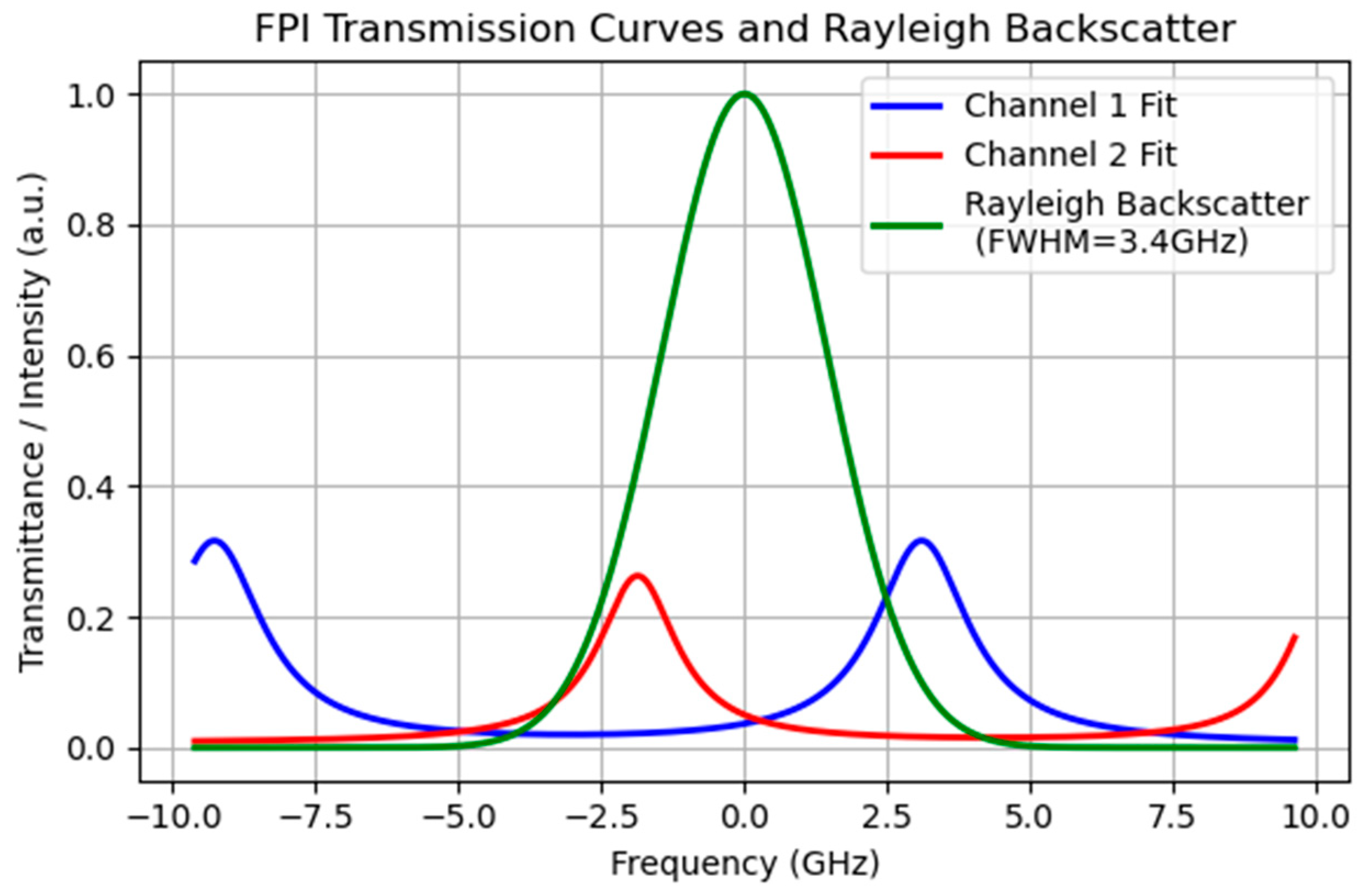
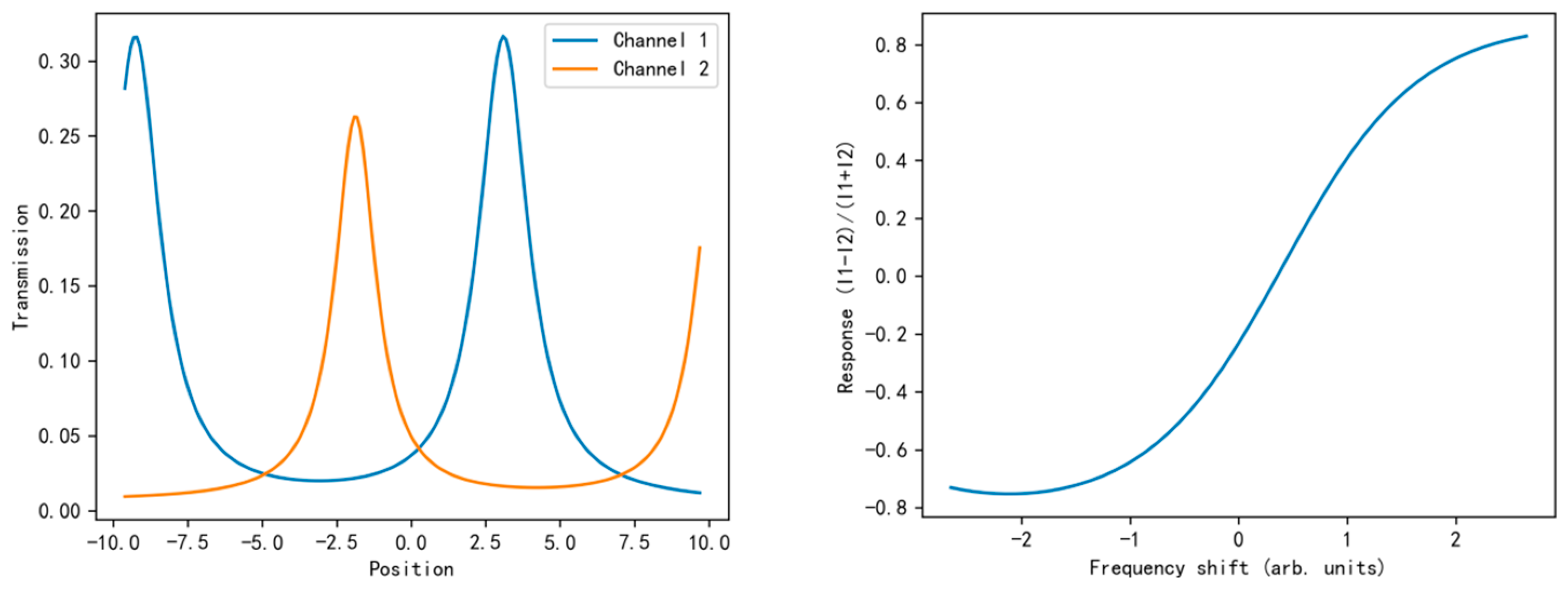
For each observation night, the transmission curves of the two FPI channels are first reconstructed from the frequency-scan calibration data. This calibration step is part of the standard preprocessing procedure in ICDL wind retrieval, because accurate Doppler inversion depends on an up-to-date characterization of the FPI transfer functions. In our implementation, rather than relying on an idealized analytical expression over the full free spectral range, we fit the measured scan within the instrument bandwidth using a double-Cauchy model. This choice is motivated by the fact that two transmission peaks are captured within the scanned interval, and the double-Cauchy form provides a more stable and accurate local representation of the measured curves for subsequent response-function construction. The double Cauchy distribution is employed, shown in Figure 2, expressed as Equation (1):

$$\mathrm{T}(\mathrm{x})\mathrm{ }\approx \mathrm{ }{\displaystyle \frac{\mathrm{A}}{1+{(\frac{\mathrm{x}-{\mathrm{x}}_{01}}{\mathsf{\gamma }})}^2}}+{\displaystyle \frac{\mathrm{A}}{1+{(\frac{\mathrm{x}-{\mathrm{x}}_{02}}{\mathsf{\gamma }})}^2}}+\mathrm{D}$$

(1)

where A represents the amplitudes of the two distribution peaks, γ is the width factor corresponding to the half-width at half-maximum (HWHM), x₀₁ and x₀₂ are the center frequencies of the two Cauchy peaks, and letter D denotes the displacement.

2.2.2. Response Function and LOS Wind Retrieval

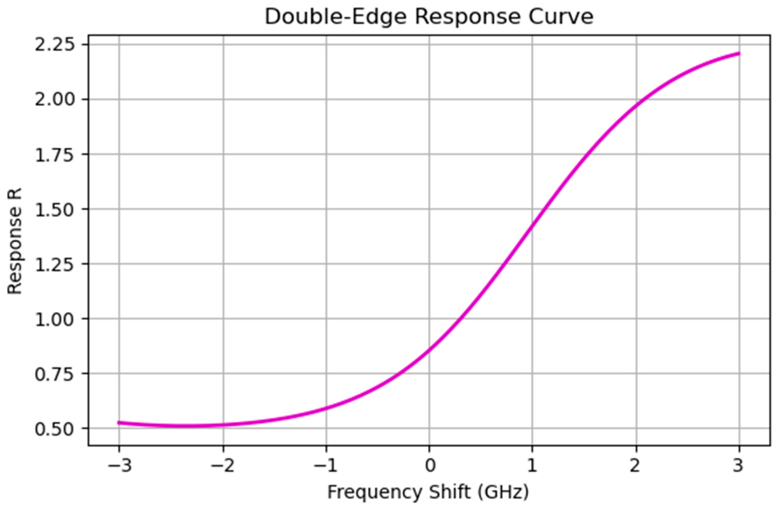
Given the reconstructed FPI transmission curves, the dual-channel response function is computed through the convolution with a modeled Rayleigh backscatter spectrum. The general forward-modeling idea follows the standard double-edge Doppler LiDAR retrieval framework [5]. However, in this study we refine the practical inversion step by introducing a revised response-function definition, rather than relying directly on the conventional channel-intensity ratio alone. This reformulation improves monotonicity and usable sensitivity over the Doppler-shift range relevant to our observations, thereby yielding a more stable mapping from measured photon counts to LOS wind velocity. The revised response function is defined as Equation (2):

$$\mathrm{R}(\mathsf{\nu })\mathrm{ }=\mathrm{ }\exp (\frac{{\mathrm{I}}_1(\mathsf{\nu })-{\mathrm{I}}_2(\mathsf{\nu })}{{\mathrm{I}}_1(\mathsf{\nu })+{\mathrm{I}}_2(\mathsf{\nu })})$$

(2)

For each observation bin, the measured photon count pair (I1(ν), I2(ν)) is converted to an observed ratio R(ν), and an interpolating function, R(ν) to Δν, as shown in Figure 3, is constructed from the simulated response curve. The Doppler frequency shift is then mapped to LOS wind velocity via the Doppler shift formula v_los = Δνλ/2, where λ is the 354.7 nm source laser wavelength of our ICDL.

2.2.3. Error Estimation and Quality Control

The uncertainty in retrieved wind velocity is governed by both system sensitivity and photon statistics. A conventional expression for the velocity error can be found in previous work [5] and is written as Equation (3):

$$\mathsf{\sigma }\left(\mathrm{v}\right)=\mathrm{ }{\displaystyle \frac{1}{{\mathsf{\Theta }}_{\mathrm{o}\mathrm{l}\mathrm{d}}\left(\mathrm{v}\right)}}\mathrm{ }{\displaystyle \frac{1}{{\mathrm{S}\mathrm{N}\mathrm{R}}_{\mathrm{o}\mathrm{l}\mathrm{d}}}}$$

(3)

where SNR_old is the combined signal-to-noise ratio of the two channels and ${\mathsf{\Theta }}_{\mathrm{o}\mathrm{l}\mathrm{d}}\left(\mathrm{v}\right)$ reflects system sensitivity. For the improved response function in Equations (4) and (5), the error expression is adjusted based on the new relation of I₁ and I₂, yielding increased robustness, especially when one channel approaches low counts:

$$\mathsf{\sigma }\left(\mathrm{v}\right)=\mathrm{ }{\displaystyle \frac{1}{{\mathsf{\Theta }}_{\mathrm{n}\mathrm{e}\mathrm{w}}\left(\mathrm{v}\right)}}{\displaystyle \frac{1}{{\mathrm{S}\mathrm{N}\mathrm{R}}_{\mathrm{n}\mathrm{e}\mathrm{w}}}}\mathrm{ }$$

(4)

$$\mathrm{w}\mathrm{h}\mathrm{e}\mathrm{r}\mathrm{e}\mathrm{ }{\displaystyle \frac{1}{{\mathrm{S}\mathrm{N}\mathrm{R}}_{\mathrm{n}\mathrm{e}\mathrm{w}}}}\mathrm{ }=\mathrm{ }{\displaystyle \frac{1}{{\mathrm{S}\mathrm{N}\mathrm{R}}_{\mathrm{o}\mathrm{l}\mathrm{d}}}}\mathrm{ }{\displaystyle \frac{2\left({\mathrm{I}}_1\right(\mathsf{\nu })\times {\mathrm{I}}_2(\mathsf{\nu }\left)\right)}{{\left({\mathrm{I}}_1\right(\mathsf{\nu })+{\mathrm{I}}_2(\mathsf{\nu }\left)\right)}^2}}$$

(5)

where $\mathsf{\sigma }\left(\mathrm{v}\right)$ denotes the estimated error, ${\mathsf{\Theta }}_{\mathrm{n}\mathrm{e}\mathrm{w}}\left(\mathrm{v}\right)$ is the sensitivity simulated from the new response function, the SNR_new is the new SNR containing the change effected by the change of $\mathrm{R}\left(\mathsf{\nu }\right)$, and I1 and I2 denote the current photon counts captured by the FPI channels. The full mathematical derivation of the new formula is detailed in Appendix A.1.

In the agent implementation, these steps are encapsulated into the following tools:

• Fitting the response curve from the FPI scan,
• Simulate a Rayleigh signal and compute the response curve
• Convert photon count profiles into LOS wind profiles
• Compute the error bar based on the SNR signal

In summary, the physical retrieval pipeline used in this work remains grounded in established ICDL wind retrieval methodology, while several practical components are refined to improve local fitting accuracy, inversion stability, and uncertainty estimation. The role of the agent is therefore not to replace the underlying physics, but to utilize this refined pipeline as a sequence of tools that can be executed through natural-language interaction.

2.2.4. Uncertainty-Weighted Wind-Profile Correction

In addition to the adjusted Doppler retrieval described above, the framework applies a profile correction with the uncertainty-weighted penalized least-squares smoother to the retrieved wind field after inversion and error estimation. This step is introduced to suppress spurious point-to-point oscillations, especially in high-altitude regions where degraded photon statistics lead to large retrieval uncertainty, while preserving the large-scale vertical structure of the wind profile.

The correction is formulated as a regularized optimization problem. Let V denote the retrieved wind profile and f the corrected profile. The corrected profile is obtained by minimizing an objective function that balances fidelity to the retrieved winds against vertical smoothness, shown in Equation (6):

$$\begin{array}{c}\underset{\mathrm{f}}{\min }\mathrm{ }(\mathrm{V}-\mathrm{f}{)}^{\mathrm{T}}\mathrm{W}(\mathrm{V}-\mathrm{f})+\mathsf{\alpha }{‖{\mathrm{D}}_2\mathrm{f}‖}^2,\end{array}\mathrm{ }\mathrm{ }$$

(6)

where W = diag(w_i) is a diagonal weight matrix derived from the estimated uncertainty at each altitude level i, with w_i = 1/σ_i2, σ_i denoting the retrieved error bar, D₂ is the second-difference operator along altitude, and α is a regularization parameter controlling the degree of smoothness.

The corresponding normal equation is expressed in Equation (7):

$$\begin{array}{c}(\mathrm{W}+\mathsf{\alpha }{\mathrm{D}}_2^{\mathrm{T}}{\mathrm{D}}_2)\mathrm{f}=\mathrm{W}\mathrm{V}\end{array}\mathrm{ }$$

(7)

In this formulation, altitude levels with smaller uncertainty retain stronger influence from the original retrieval, whereas levels with larger uncertainty are more strongly constrained by the smoothness term. As a result, the correction reduces noise-induced fluctuations in low-SNR regions while preserving the main atmospheric structure of the retrieved wind profile. The present correction is related in spirit to uncertainty-aware smoothing and regularization methods used for noisy profile stabilization [37,38,39], but is applied here with the agent’s assistance as a practical post-retrieval refinement step for Doppler wind profiles. It is then used in the subsequent evaluation and visualization steps. The effectiveness of this correction is evaluated empirically in Section 3 through comparison with external references.

2.3. Agent Architecture

The retrieval physics and uncertainty formulation define the scientific backbone of the system, whereas the agent framework contributes the orchestration, validation, and extensibility mechanisms through which these routines are executed interactively. In the present implementation, these agent functions were supported by an LLM backend accessed through the OpenAI API using a GPT-5-mini model [22].

2.3.1. Overall Architecture

The ICDL-Agent is organized as a multi-node system built around five logical nodes, a shared state object, and a centralized tool registry. Instead of treating each user instruction as an isolated prompt, the system maintains a persistent execution context across nodes and turns. This design preserves intermediate products, tool outputs, and validation results, thereby supporting both single-turn execution and iterative analytical refinement.

At runtime, the user interacts with the system through natural-language requests describing scientific analysis tasks, visualization operations, or follow-up refinements. Each request is first mapped to a structured analytical intent, then converted into a constrained executable workflow based on the currently available tools and the existing execution state. The workflow is executed step by step, with outputs validated, revised when necessary, and stored in a shared state for downstream reuse. Because intermediate products remain accessible throughout the session, later operations can build directly on previous results rather than restarting the workflow from the beginning.

The overall workflow of the agent, including the arrangement of the logical nodes, the shared state, and the centralized tool registry, is illustrated in Figure 4.

2.3.2. Functional Nodes and Shared State

The core architecture of the agent consists of five logical nodes, a shared state object, and a centralized tool registry. Each node has a distinct operational role. In this section, we first introduce four basic nodes involved in standard workflow execution, while the tool-creation node is discussed separately in the next section in connection with system extensibility. The intent detection node interprets the user request and maps it to a structured analytical intent; the planning node converts that intent into a constrained action plan; the execution node invokes registered tools and records their outputs; and the validation node checks returned results, detects failures, and triggers correction when needed. All nodes operate over a shared state object that preserves the current session context and intermediate LiDAR products.

The intent detection node serves as the entry point of the workflow. It interprets the user’s natural-language input and identifies the type of scientific operation being requested, such as curve fitting, numerical computation, or plot generation. It also determines whether the request can be satisfied using the currently available tool registry or whether additional tool creation may be required.

The planning node converts the detected intent into a structured action plan based on the current query, recent conversation history, and the available analysis tools. This structured representation reduces ambiguity in multi-step tasks and provides an explicit interface between language understanding and executable operations.

The execution node is responsible for invoking registered tools, collecting returned outputs, updating the shared state, and forwarding selected results to the user interface. In this way, numerical computation remains in explicit Python 3.9 functions, while intermediate scientific products and user-facing outputs remain available for downstream reuse.

The validation node examines execution outputs for runtime errors, malformed results, numerical inconsistencies, and interface compatibility issues. It serves as the main safeguard for result quality and execution reliability, and can trigger a bounded code-repair subroutine.

At the implementation level, each LLM-based node is controlled by an independent prompt template. These templates define the input context, allowed output structure, and node-specific constraints for intent detection, planning, tool generation, validation, and code repair. Their node-level input-output contracts are summarized in

Table 1. Node-level LLM interactions in ICDL-Agent.

LLM-Based Node	Main Input	Required Output	Main Constraints	Next Node
Intent Detection	User request, available tool list, tool argument schema, brief state context	Structured intent, use_existing_tools, needed tools, new-tool specification if needed	Tool names and argument keys must come from registry; no invented tool interfaces	Existing tools route: planning; Dynamic tool creation route: tool creation
Planning	User request, intent result, tool registry, state summary	Ordered JSON tool-call plan	Args must be executable literals; no natural-language placeholders; large arrays/dicts must be read internally from shared state	Execution
Tool Creation	New-tool specification, state summary, similar tool examples, procedural documents if needed	Complete Python function code and metadata	Fixed function signature; use get_result(state, …); return dict; avoid unsupported imports; follow LiDAR rules	Registration and planning
Validation	User request, executed plan, result summary/error summary	is_ok, issue list, user-facing summary	Check task completion, structure, numerical plausibility, physical reasonableness	Success: output response; Failed: code repair
Code Repair (Validation)	Failed function source code, traceback, expected behavior	Corrected complete function code	Preserve function signature; minimal internal changes; correct state access; no unsupported dependencies	Repair in process: re-execute; Repeated failure: explicit error report

, and their detailed description with their full prompt texts is provided in Appendix A.3.

All of these nodes operate over a shared agent state, which serves as the internal context layer of the system. The state stores the current user input and a truncated conversation history, allowing the agent to resolve referring expressions such as “this day” or “the last result” in follow-up turns. It also preserves intermediate LiDAR products, including fitted FPI transmission curves, response functions, wind profiles, wind fields, and uncertainty estimates, typically under date-aware keys so that outputs from different observation nights can be tracked and reused. In addition, a separate JSON-based memory file records the agent state after each run, enabling long-term data retrieval, inspection of historical outputs, and error traces.

2.3.3. Tool Registry and Extensibility

The tool registry serves as the central interface between the reasoning modules and the executable analysis functions. It maintains the currently available tools together with their function handles, argument schemas, and descriptive metadata, allowing the planning and execution nodes to access computational capabilities in a structured and controlled manner.

A set of predefined tools is registered at system startup, providing the initial computational backbone for standard LiDAR analysis tasks. In the present implementation, the default tool registry includes four core functions: FPI transmission-curve fitting, response-function computation, wind retrieval, and uncertainty estimation. These tools correspond to the main physical stages of the retrieval pipeline introduced in Section 2.2 and provide the initial operational basis for routine analysis requests.

The registry also supports controlled extensibility through the tool-creation node. When the currently available functions are insufficient for a user request, the agent can synthesize a new utility function and register it into the same framework used by the predefined tools. The code repair sub-module in the validation node also supports subsequent revision of dynamic tools when validation fails, allowing capability growth to remain integrated with the existing execution framework.

To improve execution reliability, all registered tools follow standardized input-output contracts. These contracts specify the required arguments, expected output types, and operational scope of each function. Such interface constraints help the planning node generate valid tool calls, reduce failures caused by malformed arguments, and make execution behavior easier to validate and audit. In addition, each tool is associated with a domain-aware description that clarifies its scientific purpose and intended usage, helping the system distinguish between functions that their name may appear similar at the syntactic level but serve different analytical roles. As a result, the registry provides not only a stable operational core for routine LiDAR analysis, but also a controlled mechanism for capability growth through tool creation and revision.

2.4. Workflows

Based on the architecture described above, each user request is processed through a structured execution workflow that either uses the existing registry directly or extends it through the dynamic tool creation. In both cases, the numerical LiDAR processing itself remains implemented in explicit Python functions for reproducibility, while the LLM is used to interpret the request, organize workflow steps, and coordinate execution with validation. The distinction between the two workflows lies primarily in whether the requested operation can be completed using the tools already available in the registry.

2.4.1. Workflow with Existing Tools Only

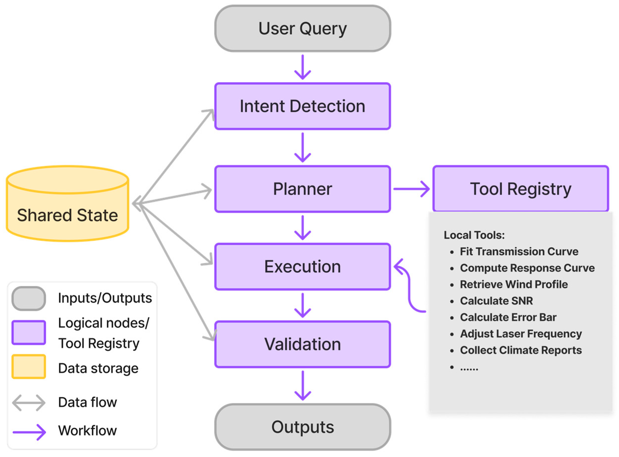
When a user request can be satisfied using the existing tool library, the agent follows a standard execution loop, illustrated in Figure 5. The process begins with intent detection, where the natural language query and recent conversation history are converted into a structured analytical request. At this stage, the system can resolve under-specified references in conversational language into executable parameters, such as dates, altitude ranges, variable types, or target operations. For example, a follow-up request may refer to a previously generated result and ask that the displayed profile be restricted to altitudes below 30 km rather than requiring the entire workflow to be reformulated.

Once the intent has been identified, the planning node constructs an executable tool-call sequence using the current registry and the shared agent state. Because the state records which intermediate products are already available, the planner can reuse prior outputs when possible instead of recomputing the full pipeline. The resulting plan is an ordered list of tool invocations with associated arguments. At this stage, the LLM is responsible for selecting tools and organizing their order, but the numerical computation remains entirely within the registered Python functions.

The execution node runs the planned tools sequentially. For each step, it retrieves the corresponding function from the registry, checks and sanitizes the supplied arguments, executes the underlying code, and stores the returned outputs in the shared state under standardized keys. This memory design allows downstream operations and subsequent user queries to access previously computed products directly.

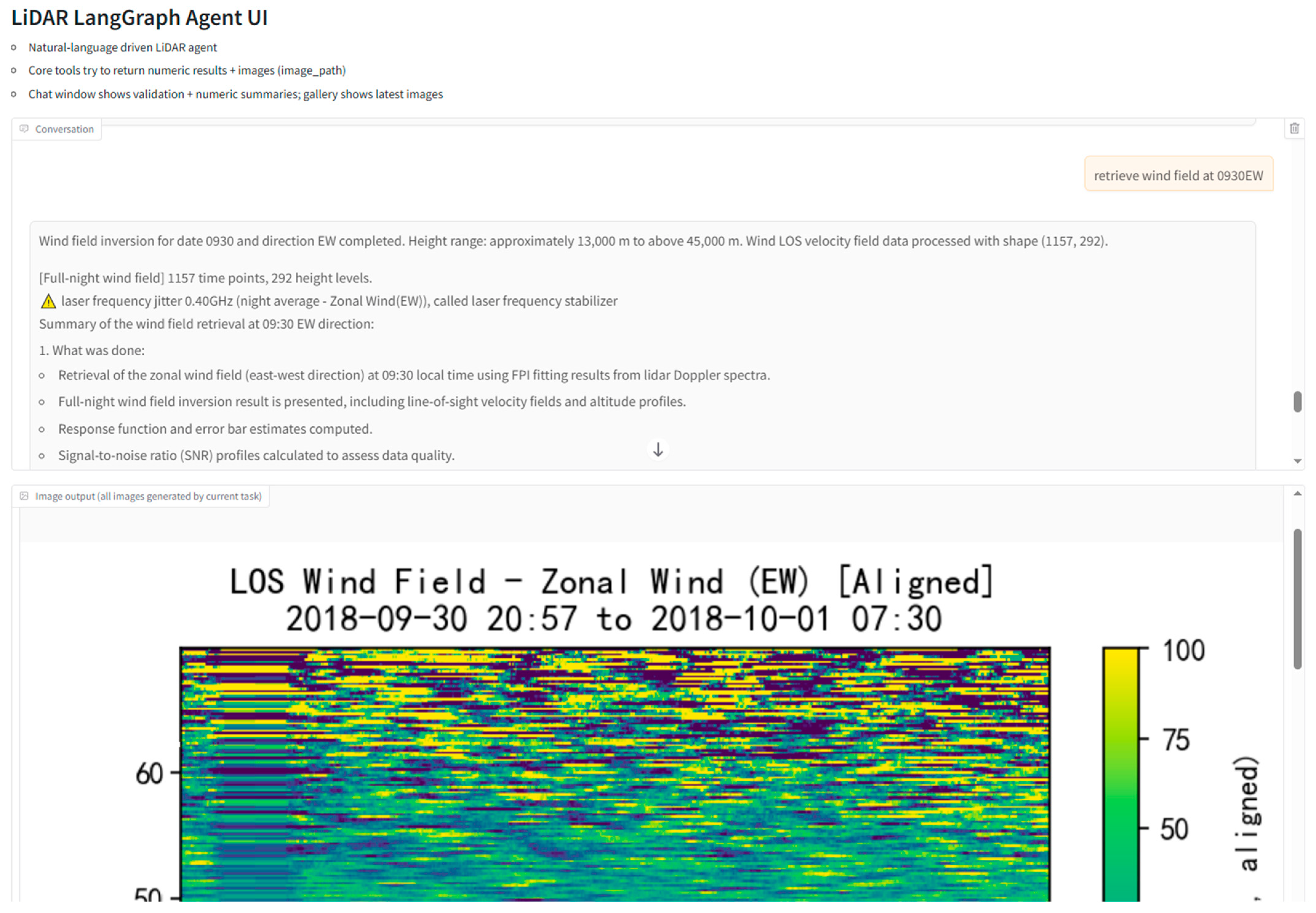
After execution, the validation node assesses whether the produced outputs are complete, technically consistent, and adequate for the original request. This assessment is based on the returned products, such as array shapes, key statistics, and diagnostic summaries. If the result is acceptable, the validated outputs, including figures, numerical summaries, and explanatory text, are forwarded to the Gradio interface for presentation (UI layout shown in Appendix A.2.4). If execution errors occur, the validation node examines the error information and routes the workflow back to the intent detection stage, where the process is restarted with the error message attached as additional context. For this workflow, the validation node does not revise any functions, because the registered tools are assumed to be operational and the failures are typically attributed to incorrect workflow planning.

In this way, the standard workflow combines structured planning, explicit numerical execution, and validated result delivery within a single reusable loop.

2.4.2. Workflow with Dynamic Tool Creation

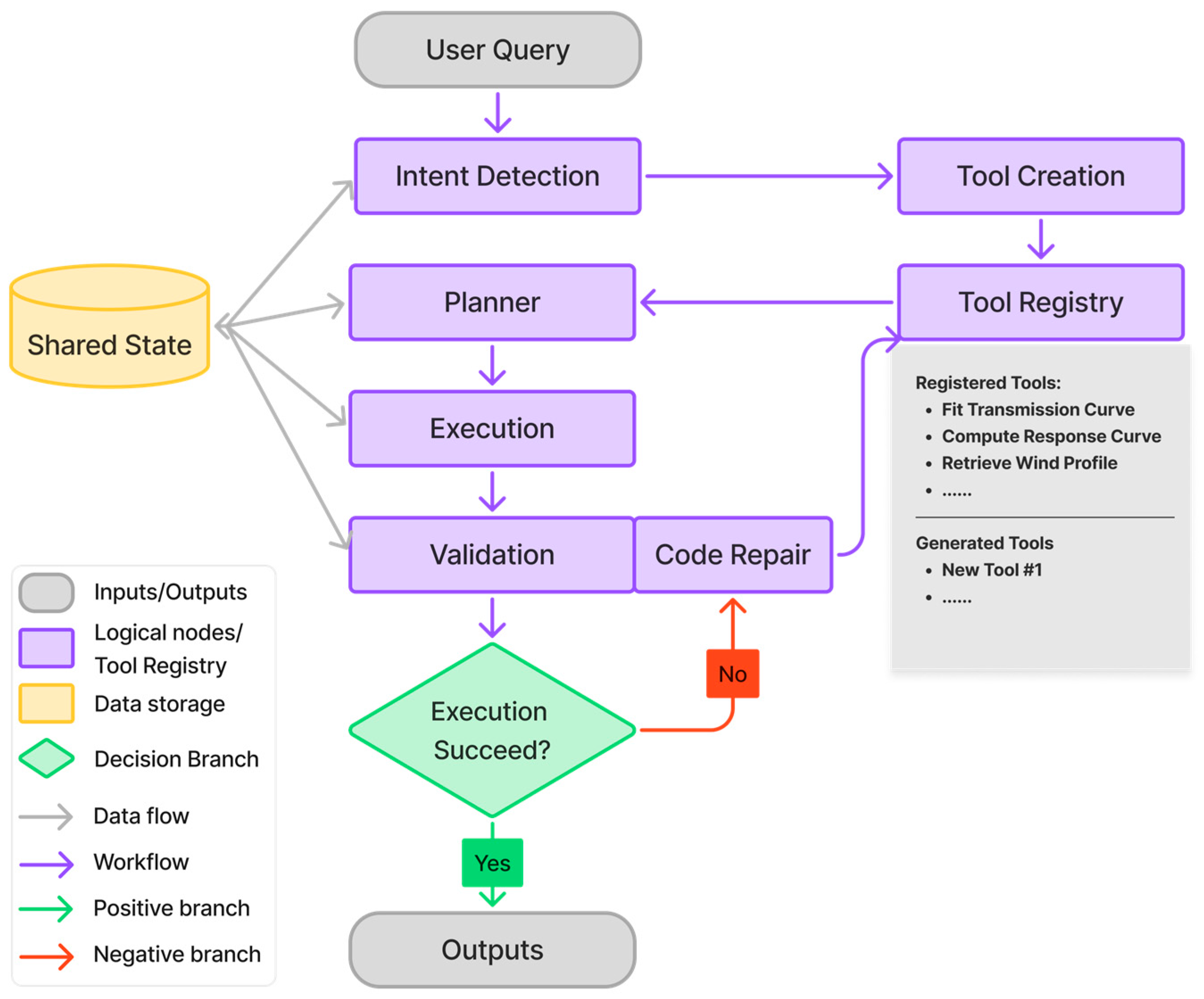
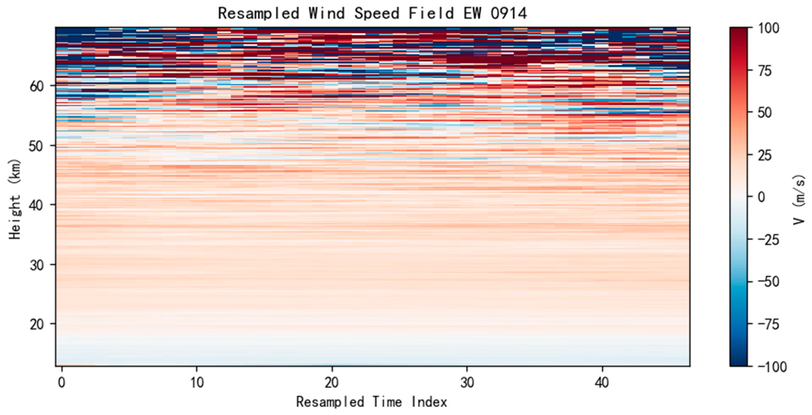
When a user request cannot be fulfilled by the currently registered tools, the workflow extends to include a dynamic tool-creation branch, as illustrated in Figure 6. This situation typically arises when the user requests an unsupported aggregation, transformation, or diagnostic operation, such as resampling an existing wind field to a new temporal resolution or generating a custom combined visualization.

As in the standard workflow, the process begins with intent detection. The system first identifies the requested task and inspects the tool registry to determine whether an existing function can perform the required operation. If no suitable tool is available, the agent constructs a structured specification describing the intended behavior, required inputs, and expected outputs, and passes this specification to the tool-creation node.

The tool-creation node then synthesizes a new Python function using the structured specification, a fixed implementation template, and selected example functions from the existing code base. For complex analytical requests, the generation context is further augmented with locally stored procedural documents. These documents do not contain executable tools themselves, but record the intended processing sequence, relevant equations, and parameter conventions for domain-specific tasks. They are retrieved only when the requested operation requires such procedural guidance, and are used together with example functions to constrain the structure and behavior of the generated tool. This mechanism is particularly useful for multi-stage scientific tasks, such as gravity-wave diagnostics, where correct execution depends not only on code templates and interface compatibility, but also on following an ordered sequence of filtering, spectral transformation, and parameter extraction steps. The generated tool is designed to read from the shared state, perform the requested computation, and return outputs in the same structured format used by the rest of the system. Once generated, the function is appended to the dynamic tool module, reloaded, and registered into the tool registry, so that it can be invoked through the same interface as the predefined tools.

After registration, the planning node is called again on the augmented registry. The newly created tool can now be inserted into a revised workflow together with existing tools. For example, the agent may first compute a full-night wind field using a predefined retrieval tool and then apply the newly created resampling tool to adjust time resolution for further plotting or comparison. From this point onward, the generated tool behaves as part of the ordinary execution pipeline.

Execution and validation then proceed in the same general manner as in the existing tool workflow, but with an additional repair pathway for the current generated tool. If the new function fails during execution or produces an invalid result, the validation node analyzes the failure and triggers bounded repair through its code repair sub-module. The revised function is then re-registered and re-executed. To prevent endless repair cycles, the number of revision attempts is limited, and repeated unresolved failures are returned to the user as explicit error reports. This closed loop confines LLM-based code synthesis and repair to a controlled execution pathway while keeping the core LiDAR processing pipeline stable and reproducible.

Although these two workflows differ in whether a new tool must be synthesized, they share the same underlying execution principles: structured intent resolution, state-aware planning, explicit tool invocation, validation of returned products, and bounded recovery when failures occur.

2.5. Execution Control

2.5.1. Prompt-Guided Execution Control

In the present framework, prompting is not used merely as a conversational interface to the language model. Its more important role is to provide execution control over an otherwise flexible generative system. In a scientific analysis setting, natural-language requests must be converted into valid workflow branches, executable tool calls, reusable intermediate products, and technically reliable outputs. For this reason, the agent is governed by a set of prompt-guided control mechanisms that constrain how requests are interpreted, how tools are invoked, and how results are accepted into the workflow.

A first layer of control is imposed through structured outputs and schema constraints. At key stages, the LLM is required to produce outputs that follow predefined formats, thereby stabilizing communication between nodes. These structured representations reduce ambiguity, narrow the action space available to the model, and make branching decisions easier to parse, audit, and reproduce.

A second layer of control concerns compatibility with data access pathways, including the shared state, LiDAR database, and tool interfaces. Because the agent operates over a persistent state object, prompts are designed to use predefined state-access functions and to encourage reuse of previously computed results whenever possible. This is particularly important in LiDAR analysis, where users often refine earlier outputs through follow-up requests. Likewise, prompts are guided to follow predefined data paths and storage conventions for LiDAR inputs and agent outputs. At the same time, prompt constraints preserve compatibility with registered tool interfaces by guiding the model to produce actions and generated functions that remain consistent with the expected data-access structures of the framework.

A third layer of control is provided by domain-aware specification. Scientific constraints are not introduced as unrestricted background knowledge, but as operational guidance embedded in workflow planning, tool generation, and result interpretation. For complex analytical tasks, as mentioned earlier, this guidance is further strengthened through the retrieval of locally stored procedural documents. This is particularly important for tasks such as gravity-wave analysis, where correct tool generation depends on following an ordered sequence of background removal, filtering, spectral transformation, and parameter extraction steps. In this sense, prompt design supports not only executable behavior but also scientific coherence within the LiDAR processing pipeline.

Finally, execution control relies on validation and bounded repair. Returned products are checked before they are accepted into the workflow, and detected failures trigger targeted correction. This correction may apply either to workflow construction or to dynamically generated tools. The number of revision attempts is limited so that unresolved failures terminate in explicit error reporting rather than endless correction loops. As a result, the system remains closer to controlled debugging and orchestration than to unrestricted regeneration. The primary execution-control layers in the LiDAR agent are detailed in

Table 2. Main execution-control layers in the LiDAR agent.

Control Layer	Purpose	Example Implementation
Workflow Routing	Select workflow branch	use_existing_tools = true
Planning	Assign tool order and args	JSON tool sequence
Data accessing	Preserve correct state and database accessing	get_result() function, shared_state[“wind_result”]
Code generation	Ensure generated tools remain executable	fixed template, fixed return format
Physical rules	Enforce physical principle	LiDAR parameters, domain formulas
Validation	Validate and correct results	data type check, numerical correctness, output check

.

Taken together, these mechanisms allow the language model to function as a constrained orchestration layer for LiDAR analysis. Prompting therefore operates at the level of execution policy: it helps translate high-level user intent into workflow behavior that remains structured, reusable, auditable, and scientifically meaningful. This control is implemented through a combination of prompting techniques, including role prompting, instruction prompting with explicit constraints, schema-constrained generation, program-aided prompting, domain knowledge injection, and dynamic few-shot prompting, rather than any single prompting strategy. Detailed node-level prompt templates, low-level formatting rules, and representative examples are provided in Appendix A.3, while the main text focuses on the design principles that affect execution reliability and scientific usability.

2.5.2. Boundaries and Error Propagation Control

The ICDL-Agent is based on the assumption that scientific LiDAR analysis can be decomposed into a sequence of modular, deterministic, and inspectable computational tools. In this framework, the LLM is not used as a direct numerical solver but as a constrained workflow orchestrator. The physical retrieval itself remains implemented in explicit Python tools based on Doppler LiDAR theories. Therefore, the correctness of physical computation is bounded through the correctness of the execution tool selection, the validity of tools and data inputs, and the validation of the output products.

The agent is most reliable when the user request can be mapped to predefined tools, or when the requested modification concerns workflow automation around existing products, such as changing plot formats, adjusting display ranges, summarizing database records, or answering questions whose required information already exists in the database. It can also support new tasks when the task can be specified through procedural document guidance. Without such guidance, however, the system is not expected to autonomously construct a scientifically complete new analysis workflow. For example, in a complex diagnostic task such as gravity-wave identification without an explicit procedural document or reliable example workflow, the agent may generate code that is syntactically executable but scientifically incomplete or inconsistent. Although the framework includes validation with predefined numerical checks, argument cleaning, state-access constraints, and bounded repair, it is still mainly LLM-based and therefore cannot be treated as a fully reliable judge of scientific correctness. It is effective for detecting many predefined or surface-level failures, such as runtime errors, missing outputs, and obvious numerical anomalies. However, it may fail when an output is structurally valid but scientifically incomplete, when values fall within plausible numerical ranges but are derived from the wrong date, direction, and height grid. For this reason, the current system should be understood primarily as a constrained workflow-automation framework rather than as an autonomous verifier of physical truth. In cases where the request is ambiguous, prerequisite products are missing, procedural guidance is insufficient, data quality is poor, or the result cannot be checked against available diagnostics such as SNR, error bars, or physical range constraints, the system may expose uncertainty, request missing context, or terminate with an explicit failure message rather than silently accepting unsupported outputs.

Error propagation is considered at two levels: the physical/numerical level and the agent/workflow level. At the physical level, errors may originate from the data and retrieval chain rather than from the deterministic execution of a correctly implemented tool. Under ideal conditions, FPI scans and photon-count profiles are processed through fixed tools, but in practice, for example, background contamination, low SNR, cloud or aerosol interference, NaNs and abnormal values, and many other data errors may propagate to affect the result. The implementation therefore includes data and numerical checks such as rejecting missing prerequisite results, removing NaN or non-finite values, preventing invalid datetime parsing, clipping extreme values for visualization, aligning wind fields to reduce laser-frequency drift, and using uncertainty-weighted correction to reduce the influence of high-error altitude levels. At the agent/workflow level, errors may propagate from ambiguous user input to wrong intent recognition, incorrect tool sequence, invalid arguments, faulty generated code, inadequate validation, and finally misleading outputs or summaries. This propagation is controlled through schema-constrained prompts, a centralized tool registry, argument cleaning, standardized shared-state keys, deterministic Python execution, validation gates, dynamic-tool code repair, limited retry, and explicit failure reporting. In practice, as shown in the failure taxonomy in Section 3.3, errors in intent recognition and planning were relatively infrequent in the tested tasks. Most unrecovered failures were concentrated in the dynamic tool-generation branch, especially when generated tools required new computation logic.

This design does not imply that the LLM agent can mathematically guarantee error-free scientific computation. Rather, it establishes a controlled execution pathway in which numerical correctness is checked through predefined rules, workflow-level errors are made explicit and traceable, and invalid outputs can be blocked, repaired, or annotated before final response generation.

2.5.3. Information Compatibility and Fusion Criteria

The framework does not treat all input sources as directly fusible data. Raw data products, such as FPI transmission scans, photon-count profiles, and CDL data, are handled as separate data types with isolated formats. Information compatibility is introduced only after the data have been converted into wind-related quantities, such as wind speeds, wind profiles, and wind fields. At this stage, products from different sources are mapped to common physical coordinates and units, including time, altitude, and wind components. For comparisons among LiDAR retrievals, ERA5, and radiosonde observations, temporal and vertical collocation or interpolation is performed before computing metrics or generating interpretations.

The spatiotemporal compatibility of LiDAR, radiosonde, and ERA5 data is handled according to their different sampling characteristics. In the present observations, the LiDAR and radiosonde measurements are geographically close, usually within approximately one kilometer, but they are not perfectly simultaneous. Radiosondes are typically launched at around 08:00 and 20:00, while the LiDAR measurement usually starts after the 20:00 radiosonde launch and ends near the 08:00 launch. Therefore, the two sources are close in location but may differ by one to several hours in time, and the final morning LiDAR data can also be affected by increasing daylight. In contrast, ERA5 provides hourly data and therefore has better temporal overlap with the LiDAR observations, but its horizontal grid resolution is about 0.25° × 0.25°, which may introduce a spatial mismatch of approximately 10–20 km relative to the local LiDAR site.

All sources also have scale differences. The LiDAR provides high-resolution local wind retrievals, with a vertical resolution of approximately 200 m and a typical useful detection range from about 13 km to 50 km, while also retaining local fluctuations in the wind field. ERA5 extends from near-surface levels to the middle atmosphere on model levels, but its vertical resolution varies with altitude, and it represents a model-computed large-scale background field rather than local small-scale fluctuations. Radiosonde data have relatively fine vertical sampling and provide independent profile-level observations, but their maximum altitude depends on balloon ascent, and the wind data used here have been filtered with smoothing. Therefore, for comparisons among LiDAR retrievals, ERA5, and radiosonde observations, temporal and vertical interpolation is performed before computing metrics. The LLM does not freely merge these heterogeneous data sources; it organizes tool calls and summaries over products that have already been converted into compatible wind-related representations.

2.6. Disclosure of Generative AI Use

Generative artificial intelligence was used in this study in two distinct ways. First, LLMs constituted an integral component of the ICDL-Agent framework itself and were used as the orchestration engine for intent detection, workflow planning, validation, and tool generation within the system evaluated in this work. These model-driven functions are part of the research object and methodology of textual, visual, and code generation. Second, generative AI was used to produce some non-data illustrative elements in selected figures and did not affect the scientific results or their interpretation. All AI-assisted content was checked, revised, and approved by the authors, who take full responsibility for the final article content.

3. Results

The results are evaluated from two complementary perspectives. The first is the scientific fidelity of the retrieved wind products, including wind profiles, full-night wind fields, and their associated uncertainty estimates. These outputs can be compared directly with both the legacy hand-written processing chain and independent external references such as ERA5 reanalysis and radiosonde observations. The second is the system-level capability of the agent as a workflow orchestration framework, including its support for conversational refinement, higher-level diagnostics, and robust execution across different task settings.

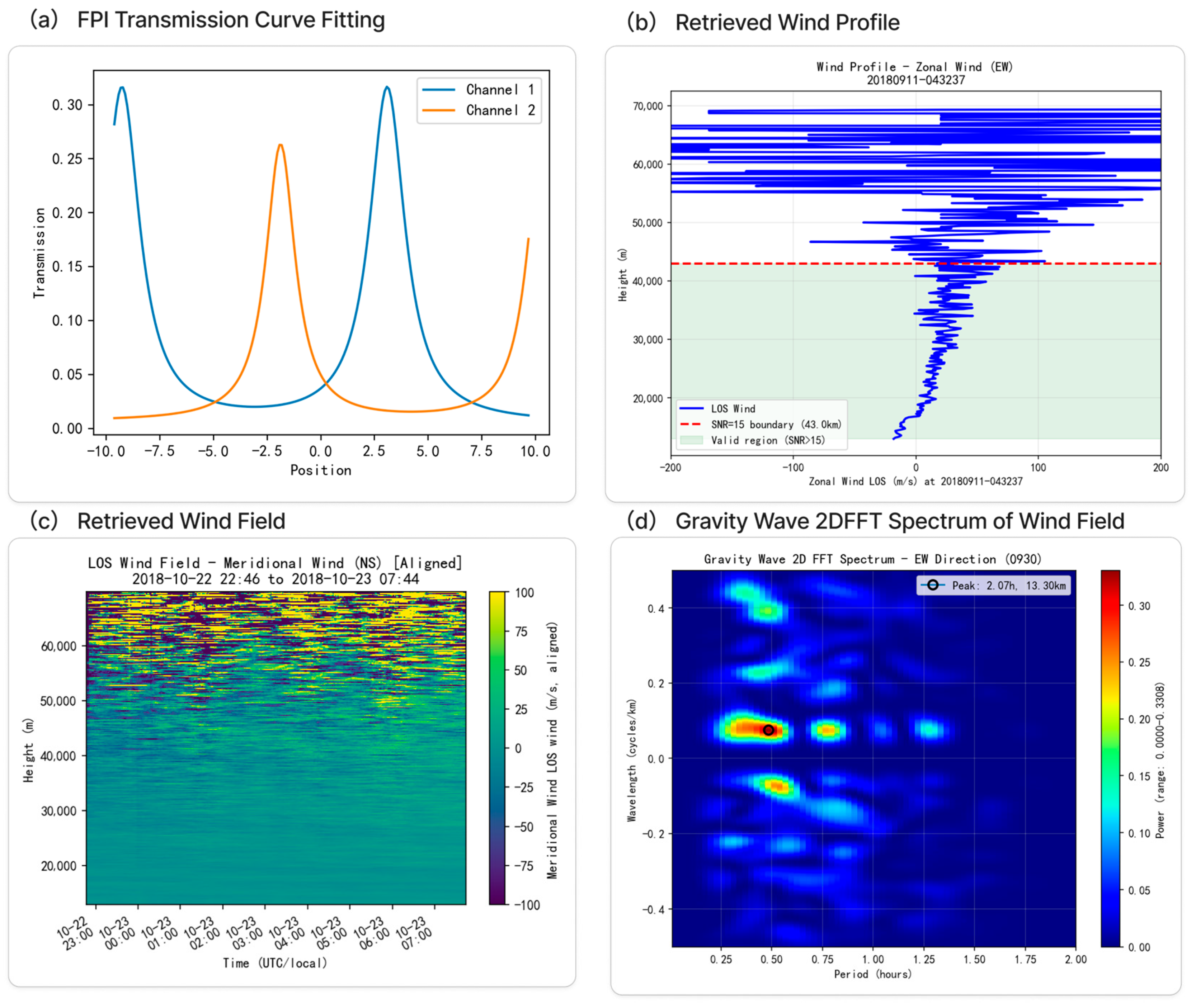
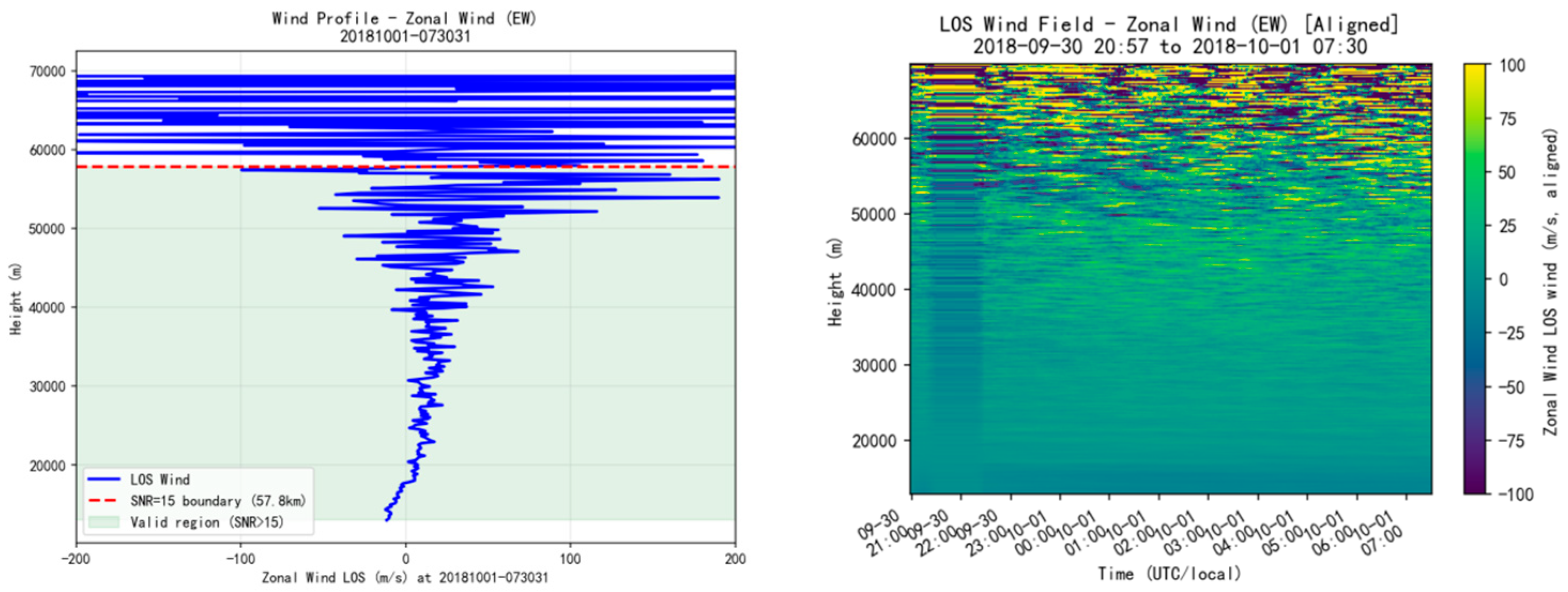
The agent produces both numerical retrieval products and user-facing analytical outputs. These include but are not limited to calibrated FP transmission fits, response functions, retrieved line-of-sight and horizontal wind profiles, full-night time-height wind fields, uncertainty estimates, comparative statistics, and natural-language summaries of the computed results. Representative examples of these outputs are shown in Figure 7.

3.1. Agent-Based Doppler Wind Retrieval

We first verify that the adjusted Doppler wind retrieval described in Section 2.2 is faithfully reproduced within the agent framework. In our implementation, the agent executes the same adjusted retrieval pipeline as the hand-written version. Retrieved wind profiles and wind fields are shown in Figure 7b,c. Comparisons on identical ICDL datasets from several full observation nights show that the agent-based implementation remains consistent with the hand-written pipeline. The two methods produce highly consistent wind structures, and their differences are mainly confined to high-altitude regions where photon counts approach the noise floor and small numerical variations are amplified. Overall, these comparisons confirm that the adjusted retrieval algorithm is accurately realized in the agent framework.

Beyond reproducing the adjusted retrieval itself, the agent framework further incorporates a post-retrieval correction stage for wind-profile refinement introduced in Section 2.2.4. This correction suppresses fluctuation in the retrieved profile according to the uncertainty estimated at different altitude levels, so that measurements with smaller errors are retained more closely, whereas points with larger uncertainties are more strongly constrained. As a result, the correction reduces spurious high-altitude oscillations caused by degraded photon statistics while preserving the large-scale background structure and maintaining a physically continuous vertical profile.

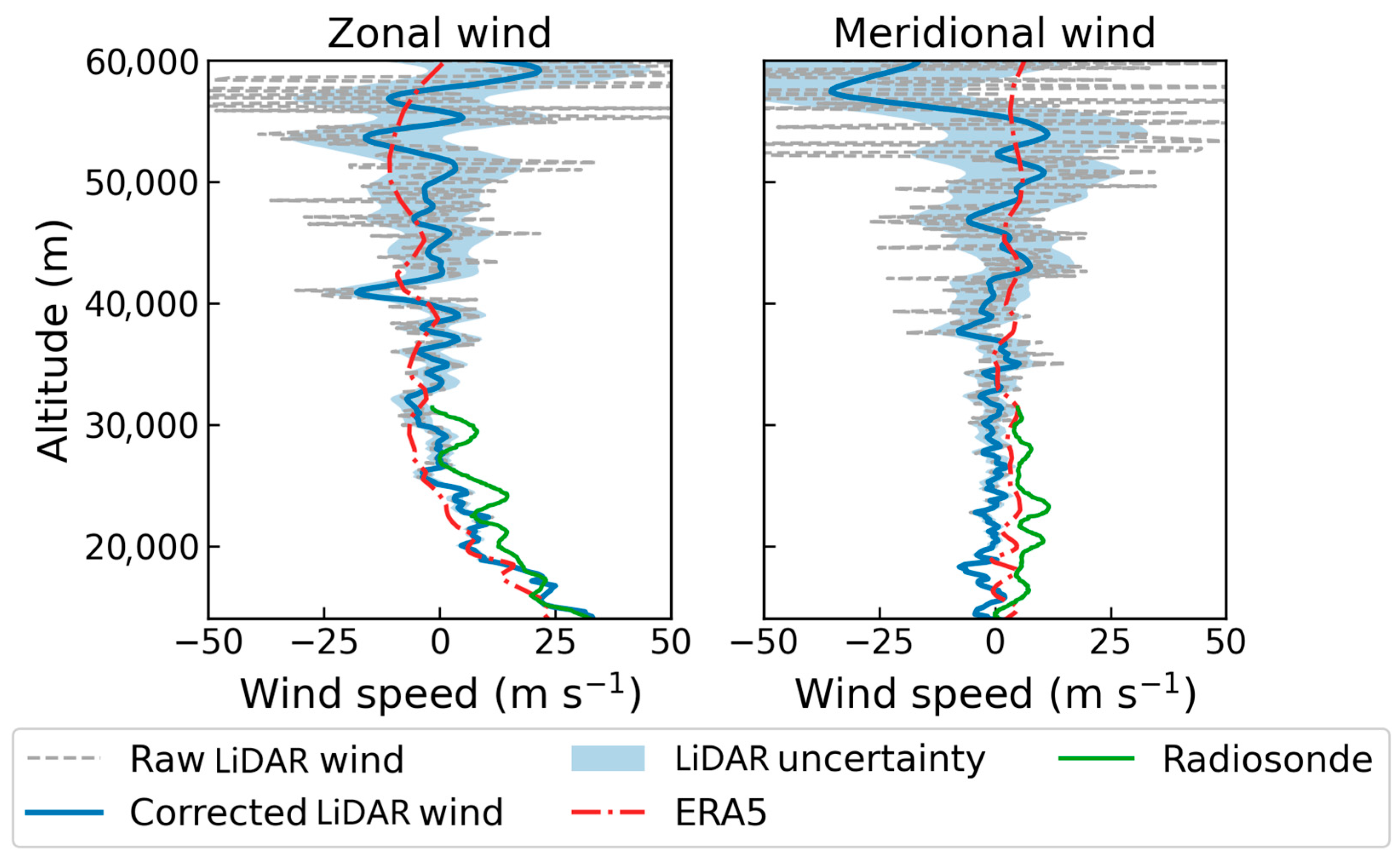
To evaluate the impact of this correction strategy, we compare three products against independent references: the traditional hand-written pipeline, the adjusted algorithm incorporating the correction stage, and external reference fields from ERA5 reanalysis and radiosonde balloon observations. A representative example of these profile comparisons is shown in Figure 8.

We first assess wind profiles against ERA5 at exactly the same time and location from all our LiDAR measurements from September to October in 2018.

Table 3. Wind Profile Evaluation Against ERA5.

Profile:	R2				MAE
Metric:	EW	NS	Wind Speed	Wind Dir	EW	NS	Wind Speed	Wind Dir
Traditional Algorithm	−0.97	−1.94	−1.58	0.20	7.25	4.41	4.78	41.46
Agent-Assisted Algorithm	0.52	0.15	0.08	0.33	3.73	2.45	3.15	33.78

reports the coefficient of determination R² and mean-absolute-error (MAE) for east–west and north–south components, as well as the joint wind speed and azimuth direction. As we can see, the traditional algorithm exhibits negative or weak R² values for the horizontal components and large absolute errors, particularly in the north–south component and in wind direction. The agent-assisted algorithm substantially improves the agreement. R² increases from −0.97 and −1.94 to 0.52 and 0.15 for the east–west and north–south components. The MAE decreases from 7.25 to 3.73 for the east–west component and from 41.41 to 2.45 for the north–south component. Errors in wind speed and direction are also reduced, with the magnitude error dropping from 4.78 to 3.15 and the directional error from 41.46 to 33.78 degrees. These results indicate that the LLM-driven corrections bring the retrieved wind profiles significantly closer to the wind trend profile represented in ERA5 model data, while still retaining the finer variability resolved by the LiDAR.

We then evaluate the above results against balloon observations. In this case, the LiDAR fields are interpolated to the radiosonde times and altitudes, and R² and MAE are computed for each product. As shown in

Table 4. Wind Field Evaluation Against Radiosonde.

Profile:	R2				MAE
Metric:	EW	NS	Wind Speed	Wind Dir	EW	NS	Wind Speed	Wind Dir
Traditional Algorithm	0.63	−1.08	0.52	−0.13	2.95	2.15	2.55	27.04
Agent-Assisted Algorithm	0.80	−0.26	0.73	0.11	2.31	1.72	2.04	21.44
ERA5	0.19	−2.20	−0.09	−0.32	5.30	4.06	5.05	37.4

, the agent-assisted algorithm again outperforms both the traditional algorithm and the ERA5 model in calculating the wind trend. For the east–west component, R² increases from 0.63 to 0.80, and the mean absolute error decreases from 2.95 to 2.31. For the north–south component, R² improves from −1.08 to −0.26, and the mean absolute error decreases from 2.15 to 1.72. Errors in wind speed and direction follow the same trend. The agent-assisted winds exhibit lower MAE than ERA5 in all metrics, while maintaining higher correlation with the radiosonde profiles.

Overall, these comparisons show that the ICDL-agent assistance significantly outperforms the traditional handwritten pipeline. It systematically reduces the noise-induced fluctuation, especially in regions with low SNR signals, and improves the accuracy of the wind profile retrieval with different references. At the same time, small-scale structures that are absent from ERA5 data but supported by the LiDAR and radiosonde measurements remain consistent. This suggests that the agent is able to incorporate the LLM-proposed statistical corrections in a way that respects the underlying physical signal and improves the overall reliability of the retrieved wind profiles.

3.2. Advanced Agent Performance

In addition to the quantitative evaluation presented above, the agent also exhibits capabilities that are better illustrated through representative qualitative cases than through summary metrics alone. The examples in this section are therefore intended to demonstrate how the framework supports interactive refinement, derived diagnostics, and physically grounded interpretation within a stateful LiDAR analysis workflow. These cases illustrate the broader analytical functions enabled by the agent once the numerical workflow has been successfully executed.

3.2.1. Interactive LiDAR Analysis Through Conversational Refinement

One important capability of the framework is support for interactive LiDAR analysis through multi-turn conversational instruction. Rather than requiring the user to specify all analysis settings in a single request, the system allows the workflow to begin from a broad scientific query and then be progressively refined through follow-up instructions. Because intermediate products are preserved in the shared state, these follow-up requests can be interpreted relative to prior computations instead of being treated as entirely new tasks.

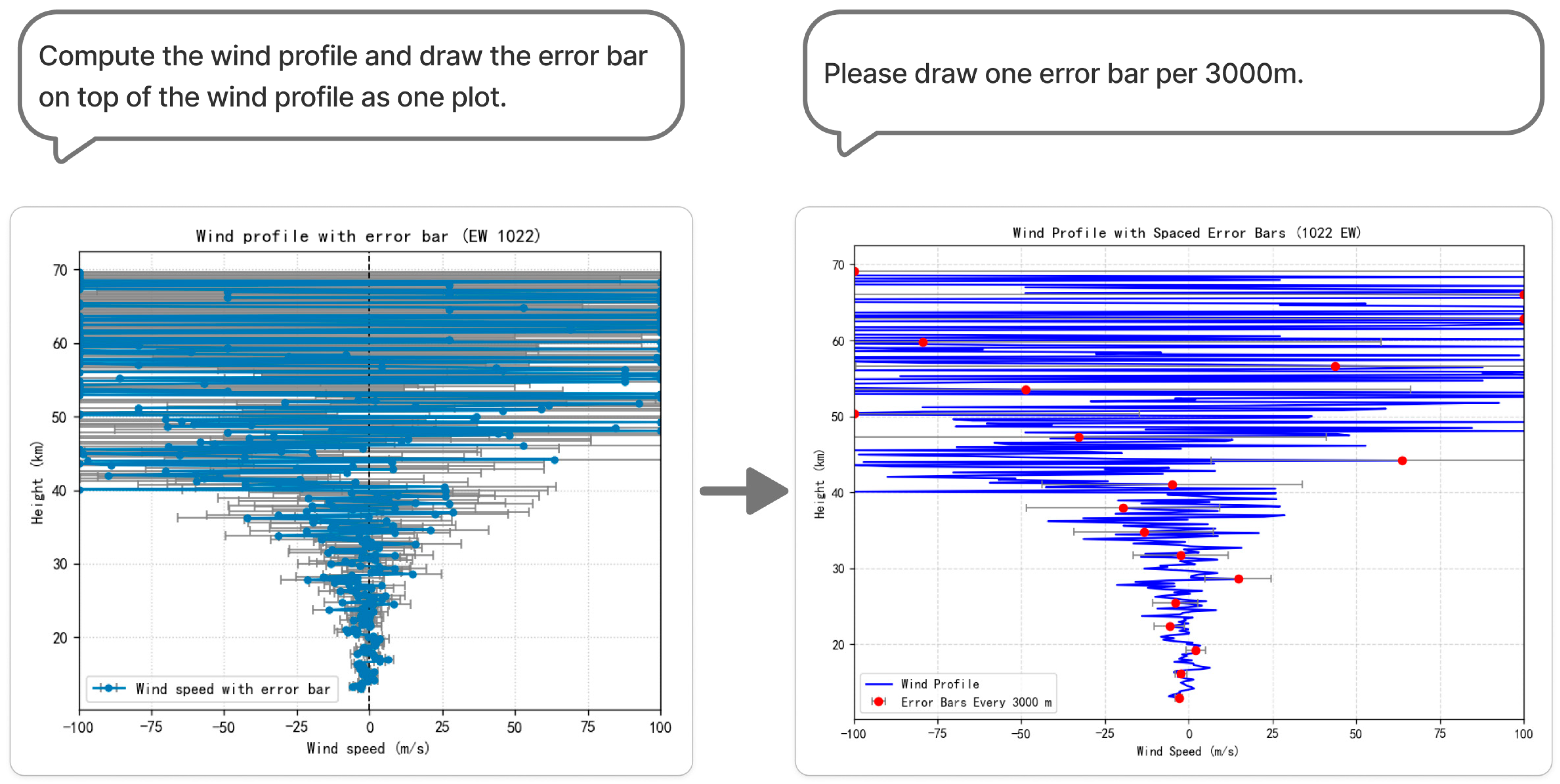
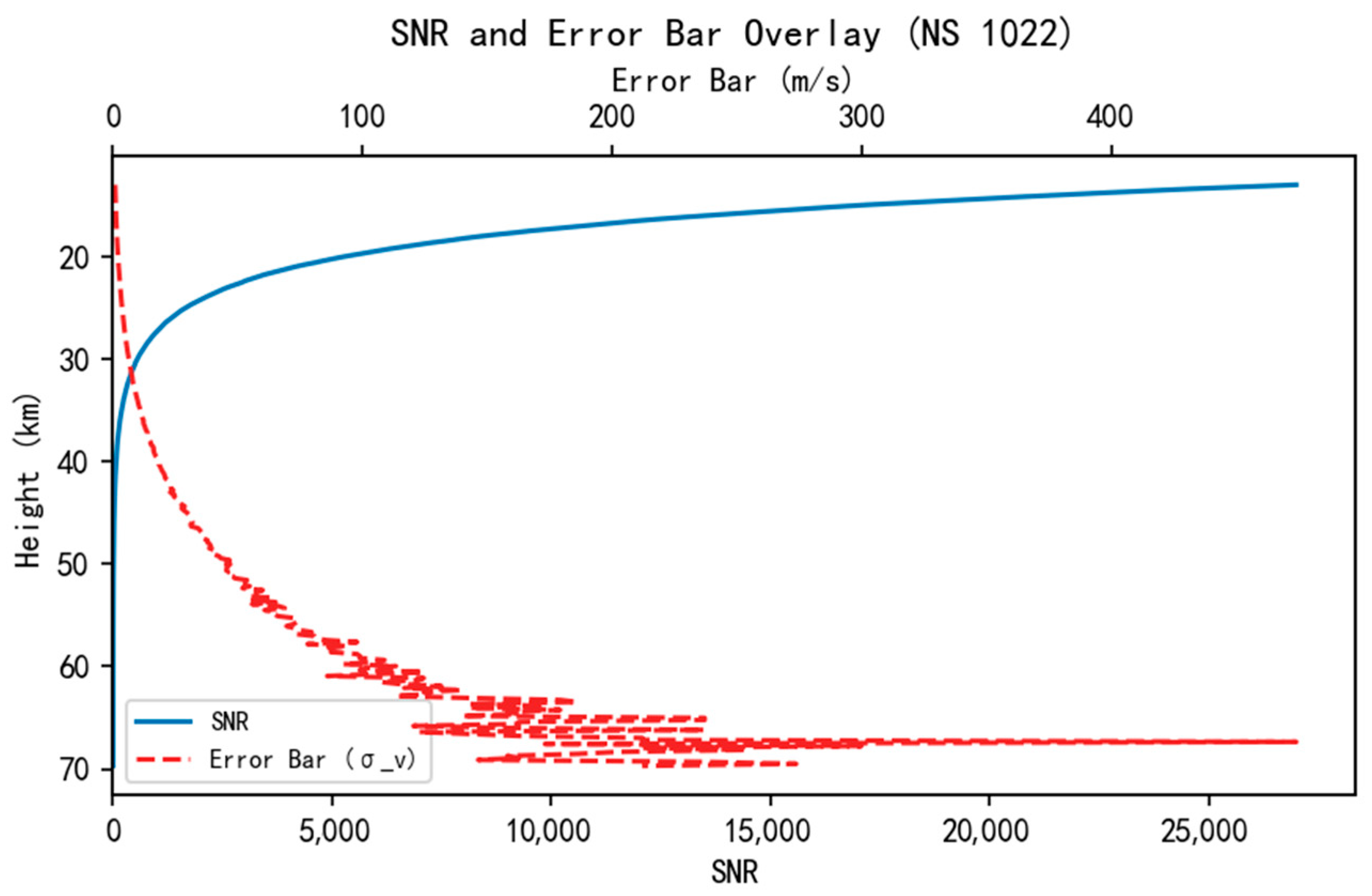
A representative example is shown in Figure 9. In this case, the user first requested that the agent retrieve the wind profile and corresponding error bars at a selected time and generate a single plot with the error bars overlaid on the profile curve. Since no existing tool in the registry directly supported this combined operation, the agent invoked the tool-creation node to synthesize and register a new plotting function. The initial result displayed error bars at every height bin, which made the profile curve visually difficult to inspect. The user then refined the request by specifying that the error bars were overly dense and should be shown only once every 3 km. The agent interpreted this as a modification of plotting density, revised the tool behavior, and returned a clearer figure with reduced visual clutter.

This case illustrates that the framework supports not only direct execution of LiDAR tasks, but also user-guided adjustment of generated outputs within the same analytical session. More generally, the same interaction pattern can be extended to other follow-up operations, such as restricting altitude ranges, changing temporal resolution, adjusting visualization settings, and so on. At the same time, the effectiveness of this interaction mode still depends on an accurate interpretation of user intent. In some cases, the agent may only partially understand a follow-up request when the instruction is expressed in ambiguous conversational language. Overall, the agent provides a more flexible interface for exploratory analysis than a static script-based workflow, while still grounding follow-up operations in previously computed products.

3.2.2. Higher-Level Diagnostics

A second qualitative capability of the framework is its support for higher-level diagnostics built on previously retrieved wind products. Beyond routine retrieval and plotting, the agent can assemble multi-step workflows for comparative wind analysis, summary statistics, and perturbation-based diagnostics. In these cases, the framework reuses wind profiles and wind fields already stored in the shared state and applies additional analysis tools to generate outputs that are more directly relevant to scientific interpretation.

In addition to routine wind-retrieval-related computations, the agent can carry out higher-level diagnostics that combine numerical analysis with physical interpretation. One important capability is climatological comparison. For autumn observations at mid-latitudes over China, aggregated lidar winds above the tropopause often show persistent westerlies in the lower stratosphere, with nightly mean zonal velocities commonly exceeding 20 m/s near 30–40 km. When the agent is requested to do a climatological diagnostic under the current measurement, it reports both the quantitative anomaly and a physically grounded explanation. A specific example is detailed in Appendix A.2.3. In this way, the framework places individual LiDAR observations within a broader seasonal and climatological context rather than treating each night as an isolated case.

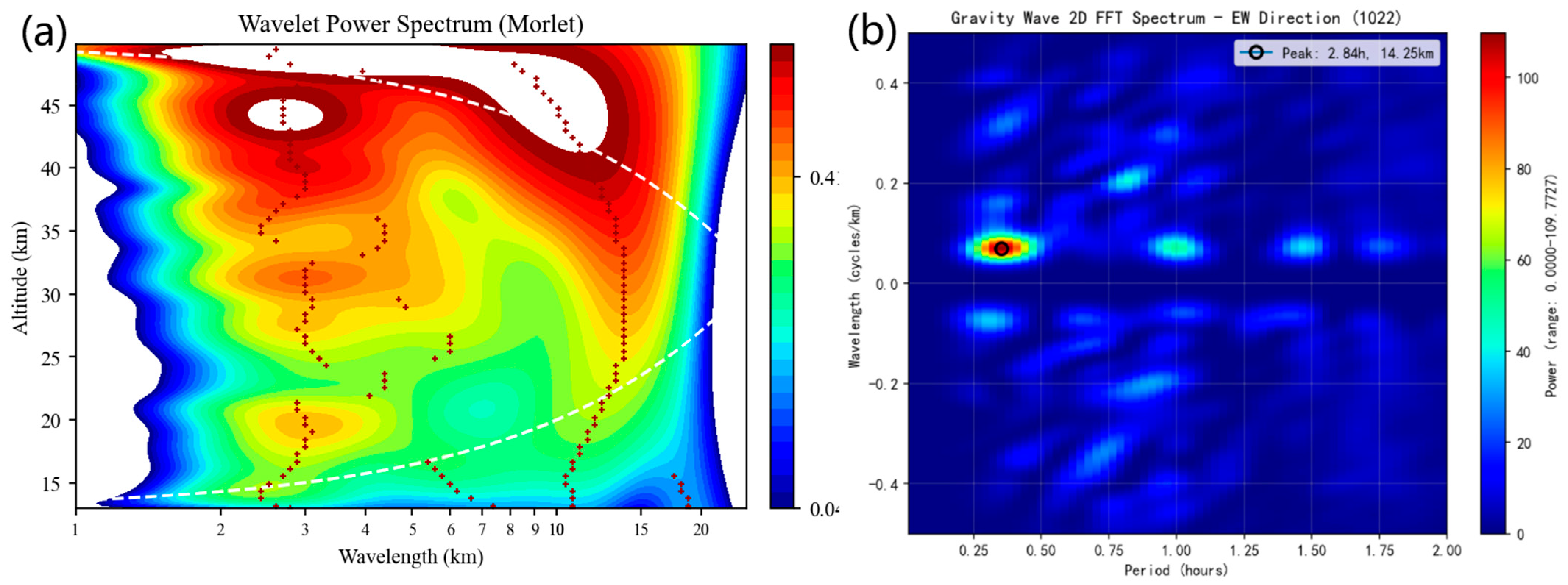
A more complex example is gravity-wave-related analysis. Starting from the retrieved wind field, the framework can perform background removal, vertical band-pass filtering, and temporal high-pass filtering, followed by spectral analysis in both Fourier and wavelet domains. This gravity-wave workflow is generated from the tool-creation process that can additionally retrieve a locally stored procedural document that records the intended analysis steps, relevant equations, and parameter conventions for gravity-wave diagnostics. This document-guided generation process is combined with example code from the existing tool base, so that the generated tool is constrained both by executable interface requirements and by domain-specific workflow knowledge.

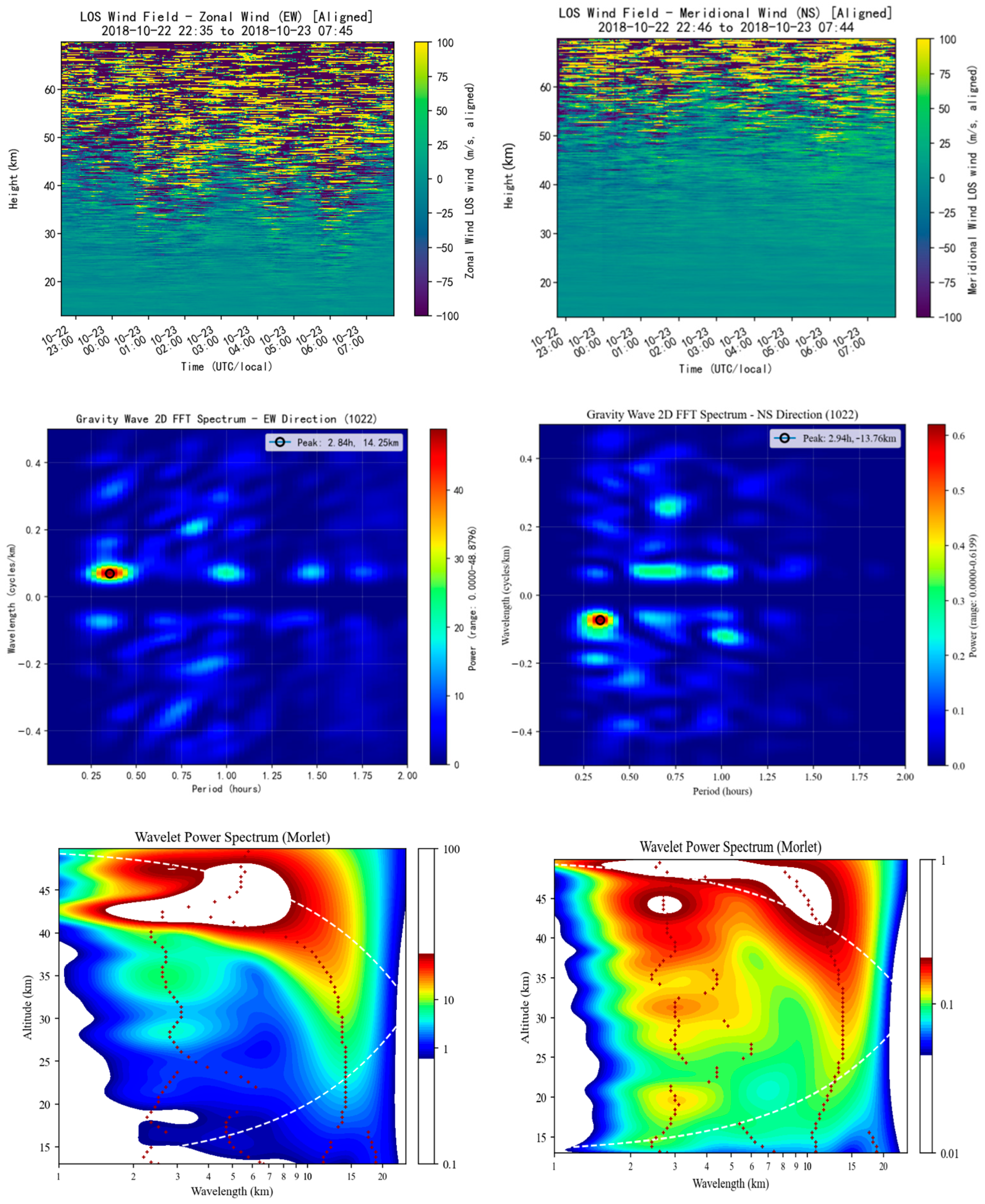
As shown in Figure 10, the resulting workflow automatically generates both a two-dimensional Fast-Fourier-Transformation (FFT) spectrum and a wavelet power spectrum for the east–west wind field on 22 October. In this case, the agent returned the summary: “Gravity wave analysis for date 1022 in EW direction completed. Gravity wave detected, key parameters: period = 2.84 h, wavelength = 14.25 km.” These retrieved scales fall within the range expected for lower-stratospheric gravity-wave activity and are consistent with the enhanced perturbation power shown in Figure 10, where red markers indicate possible gravity wave occurrence in the wavelet power spectrum and the dominant peak is labeled in the FFT spectrum. More importantly, the analysis is grounded in computed wind fields, filtering steps, spectral transforms, and parameter extraction, rather than in free-form description alone.

These examples show that the framework does more than return raw numerical outputs or standalone plots. It combines domain-specific tools for Doppler wind LiDAR with the reasoning and explanation capabilities of a large language model, enabling users to request not only retrieval results and derived diagnostics, but also comparative wind analysis, process-oriented interpretation, and gravity-wave-related diagnostics. These cases illustrate the broader analytical scope enabled by the agent, which would otherwise require substantially more manual inspection and post-processing.

3.2.3. Transferability

A further qualitative demonstration of the framework is its transferability to different remote sensing instruments. Although the main body of this study focuses on ICDL, the overall agent architecture is not tied to a single fixed retrieval chain. Instead, workflow planning and tool generation are conditioned by injected domain knowledge, equations, and data types. This makes it possible to adapt the same framework to a CDL task by supplying only the corresponding documentation and the CDL raw data. This document specified the relevant data path, the structure of the CDL data format, the relevant formulation, and the required output conventions; detailed information is provided in Appendix A.4.2. Guided by this instrument-specific knowledge, together with existing ICDL tools of similar functionality used as references, the agent automatically generated a new retrieval tool for CDL wind profile processing.

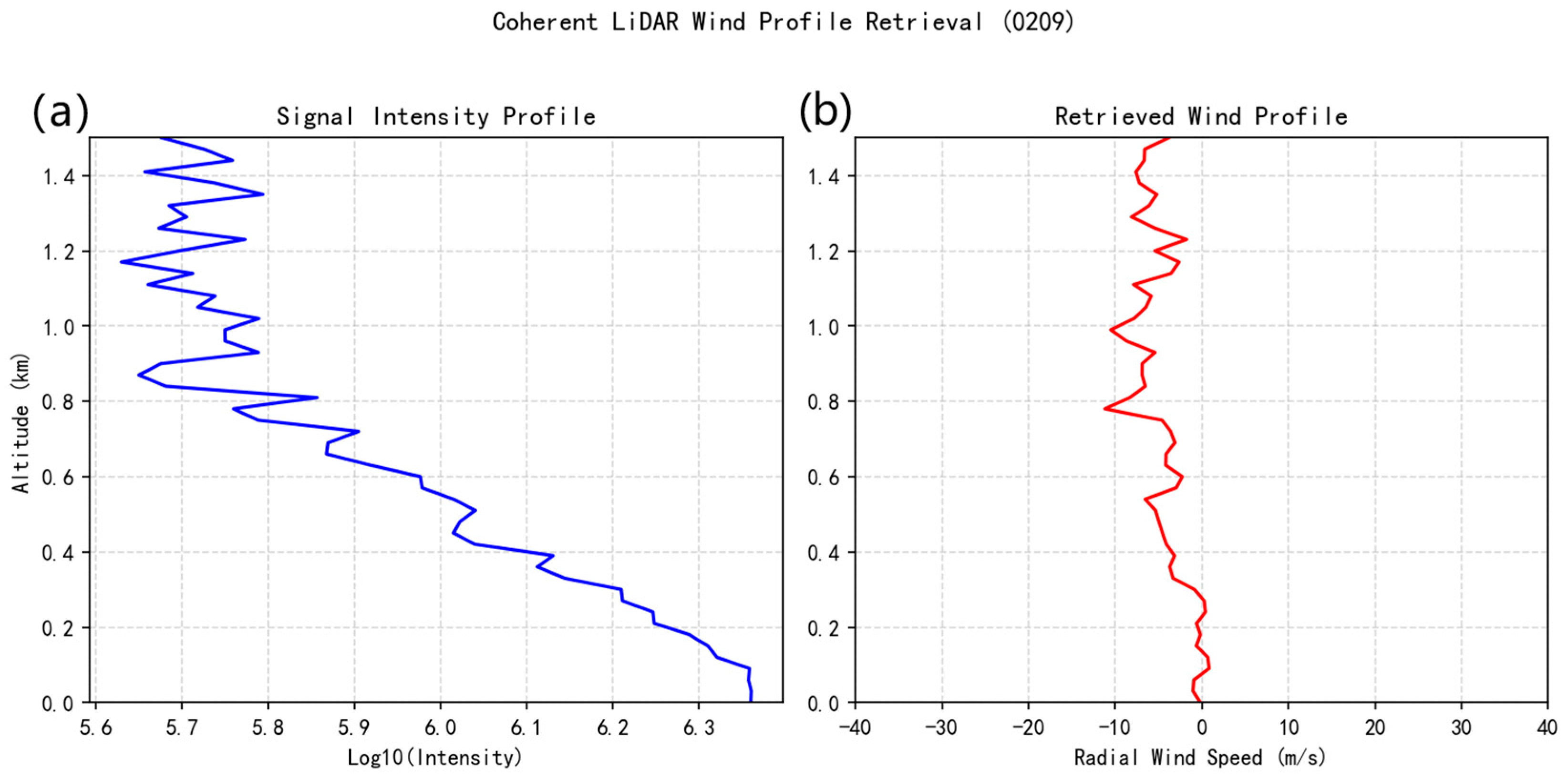
The CDL measurement data take the form of a spectral-matrix-type signal representation, which differs substantially from the photon-count-based ICDL data structure and retrieval procedure introduced in the previous sections. Nonetheless, as shown in Figure 11, the generated tool successfully produced a CDL wind profile consistent with the result from the corresponding hand-written pipeline, together with the associated signal profile used as a reference for output fidelity. This result suggests that the proposed framework is not limited to a single instrument-specific implementation, but can be extended to other remote sensing instruments when appropriate domain knowledge and procedural guidance are provided.

The present CDL example is intended as a qualitative demonstration of transferability rather than a full benchmark, but it indicates that the framework has strong potential for broader instrument adaptation.

3.3. Agent Behavior, Planning Quality, and Robustness

3.3.1. Task Success Rate, Ablation Baseline, and Failure Taxonomy

To quantify the ICDL-Agent’s behavior as a decision-making system, we evaluate task-level success rates across three settings: single-tool tasks without tool creation, multi-tool tasks without tool creation, and tool-creation tasks with repair. We curated a test set of 50 tasks spanning calibration, single-profile retrieval, full-night wind-field construction, temporal aggregation, summary statistics, and related analytical requests. Each user query was treated as a task with an expected output type and a reference implementation based on hand-written scripts. A task was counted as successful if (i) the workflow completed without unrecovered runtime errors; (ii) the numerical output agreed with the reference within a predefined tolerance when applicable; and (iii) the returned text and visualization adequately addressed the user request.

Table 5. Task Success Rate for Assorted Task Settings.

Task Category	Tasks	Model	Execution Success Rate	Result Correctness Rate	Common Failure Modes
Single-tool	10	GPT-5-mini	10/10 (100%)	10/10 (100%)	NA
		Qwen-plus	9/10 (90%)	7/10 (70%)	missing prerequisite data (1) E2; incomplete/non-interpretable output (2) E4
Multi-tool	10	GPT-5-mini	10/10 (100%)	9/10 (90.0%)	data missing (1) E0;
		Qwen-plus	8/10 (80%)	5/10 (50%)	incomplete workflow output (3); invalid argument or missing prerequisite (2) E2
Tool creation	30	GPT-5-mini	17/30 (56.7%)	16/30 (53.3%)	ambiguous intent (2) E1; missing Args (1) E2; data type misalignment (5) E3; import error (2) E0; missing prerequisite data (3) E2; physical infeasibility (1) E4
		Qwen-plus	24/30 (80.0%)	15/30 (50.0%)	state/interface mismatch (3) E3; physically implausible output (4) E4; incomplete output (4) E2/E4; unit/argument mismatch (2) E3/E4; dependency/tool error (2) E3

summarizes task-level performance across the three workflow settings. For the 10 single-tool tasks, the agent achieved perfect performance, with an execution success rate of 10/10 and a result correctness rate of 10/10, both equal to 100%. For the 10 multi-tool tasks, which require chaining outputs from one function into subsequent operations, the agent also achieved an execution success rate of 10/10 (100%), while the result correctness rate was 9/10 (90.0%). The single incorrect case was associated with missing data in the underlying database rather than a failure of workflow composition. For the 30 tool-creation tasks, the agent achieved an execution success rate of 17/30 (56.7%) and a result correctness rate of 16/30 (53.3%). The observed failures in this setting were heterogeneous in origin, including ambiguous intent, missing required arguments or prerequisite inputs, data-type misalignment in generated tools, import-related errors, and physically infeasible outputs detected during validation.

To evaluate whether the framework depends exclusively on a proprietary model backend, we further repeated the task-level evaluation using Qwen-plus while keeping the same task set and evaluation criteria. The Qwen-plus backend achieved 9/10 execution success and 7/10 result correctness on single-tool tasks, 8/10 execution success and 5/10 result correctness on multi-tool tasks, and 24/30 execution success with 15/30 result correctness on tool-creation tasks. The relatively high execution success rate of Qwen-plus, especially in tool-creation tasks, should be interpreted with caution. Some runtime-level failures observed in earlier GPT-based runs had already led to small refinements in the prompt templates and system structure, and these refinements were retained when the Qwen-plus evaluation was conducted. Therefore, the improved execution success rate mainly indicates fewer runtime errors and implementation-level crashes under the revised system, rather than stronger scientific correctness.

In contrast, the result correctness rate of Qwen-plus remains lower than that of GPT-5-mini in single-tool and multi-tool settings, and is only comparable in the tool-creation setting. This suggests that Qwen-plus can often execute or generate runnable workflows, but is less stable in producing complete, physically interpretable, and task-satisfying outputs. Typical issues include incomplete outputs and physically implausible results. It should also be noted that the prompt templates and user intents in our evaluation contain both Chinese and English, with a roughly balanced bilingual context. This may influence model behavior, and Qwen-plus may have advantages in contexts of Chinese instruction. Finally, the reported statistics are based on filtered results from multiple runs. Non-ideal interruptions that were not directly related to the agent design, such as request timeouts, missing Python dependencies, or crashes that interrupted all subsequent tasks, were excluded or treated separately before computing the final task-level rates.

To provide a stronger baseline than zero-shot LLM prompting, we further evaluated an ablated version of ICDL-Agent in

Table 6. Ablation baseline without validation and repair.

Task Category	Tasks	Execution Success Rate	Failure Modes
Single-tool	10	10/10 (100%)	NA
Multi-tool	10	9/10 (90.0%)	Validation/runtime(1) E4;
Tool creation	30	14/30 (56.7%)	Validation/runtime(13) E4; Tool creation(3) E3;

, in which the validation and repair mechanisms were disabled. We maintained the rest of the components, as they are mandatory for the agent to remain a runnable workflow system. This ablation study therefore focuses on the reliability contribution of the validation node. Compared with the full ICDL-Agent, the ablated system shows similar performance on simple single-tool and multi-tool tasks, but only a moderate decrease in the tool-creation settings, where execution success drops from 17/30 in the full system to 14/30 after validation and repair are removed. To be noticed, since the validation node is removed in this ablation, result correctness cannot be assessed automatically using the same validation-based criterion as in the full system. Looking into the failure modes, it suggests that the current validation and repair module mainly helps resolve runtime-level failures and debugging issues rather than numerical and scientific correctness. In addition, when the same LLM is used for both workflow generation and result validation, its ability to identify its own scientific or logical errors is limited. Alternative validation designs, such as using a separate LLM or an external verifier, are outside the scope of this study. The ablation also shows that the main bottleneck of the ICDL-Agent is not routine tool selection, but the ability to detect, repair, or safely reject failures introduced by dynamic tool generation.

To better characterize unsuccessful cases, we grouped the observed failures into five categories according to their primary source in

Table 7. Primary failure modes observed across incorrect results.

Error Type	Definition (Primary Cause)	Failures	Fraction of Failures	Typical Triggers
E0 External Factors	Non-systematic errors	2	2/15 (13.3%)	imported uninstalled module, missing data
E1 Intent	Ambiguous or wrong intent parsed	2	2/15 (13.3%)	misinterpret, typos, human expectation mismatch
E2 Workflow	Plan/sequence missing step or precondition	4	4/15 (26.7%)	missing prerequisite data, missing arguments;
E3 Tool creation	Mismatched functionality or an implementation mistake	6	6/15 (40%)	module import failure; missing arguments
E4 Validation	Validation or runtime errors	1	1/15 (6.7%)	physically implausible outputs

, spanning external factors, intent interpretation, workflow composition, tool creation, and validation handling. Across the 15 failed tasks, the dominant error source is E3 tool-creation failure, accounting for 6/15 cases (40.0%). These cases arise when newly synthesized tools contain unexpected functionalities, interface inconsistencies, or implementation errors, even if the tool generation itself appears to complete successfully. The second largest category is E2 workflow failure, with 4/15 cases (26.7%), typically caused by missing prerequisite inputs or incomplete argument passing.

Taken together, the two tables show that the framework is already highly reliable when user requests can be resolved through predefined tools or standard validated workflows, and that most of the remaining difficulty is concentrated in less constrained settings that require new tool synthesis. At the same time, the aggregate failure rate in the tool-creation setting should not be interpreted as arising solely from deficiencies in tool generation itself. Some failed cases are attributable to external factors, ambiguous intent, or validation mechanisms (which correctly reject unreliable outputs, detailed in the next section). It should also be noted that the present evaluation was conducted in a batch, single-turn setting for reproducibility, and therefore does not capture the potential benefit of multi-turn clarification. In practical interactive use, some failures associated with ambiguous intent or missing arguments could likely be resolved through follow-up dialogue and iterative replanning. Within this broader context, the most consequential remaining bottlenecks are tool-creation robustness and prerequisite-aware workflow coordination, especially when generated code must interact consistently with the shared computational state and existing tool interfaces. These results therefore suggest that the most effective improvements will come from stronger interface constraints for generated tools, better prerequisite inference and argument checking, and tighter coupling between planning, execution, and validation.

3.3.2. Failure-Case Analysis

Representative failure cases further clarify the limitations of the current framework beyond the aggregate statistics in Table 7. Because E3 tool-creation failures and E2 workflow failures account for the largest fractions of unsuccessful tasks, we first discuss these two dominant categories through representative examples. We then examine two lower-frequency but conceptually important cases, E1 and E4, because they reveal limitations that are not fully reflected by failure counts alone. Each case is discussed not only as an example of failure, but also as a pointer to a possible improvement strategy or an evaluative discussion.

A typical E2 error arises when the workflow fails to infer the prerequisite computation required by a newly requested analytical task. For example, when the user requests a wind-field plot restricted to a certain time interval, such as 23:00–23:40, the system generates a new tool for time-range selection but does not plan the preceding wind-field computation required to supply its input. This example shows that the current workflow construction mechanism may still miss necessary upstream computations even when the intended analytical direction is reasonable. A practical improvement would be to manage repair and replanning more adaptively in prerequisite-sensitive cases. The current framework already supports repair-based replanning, but in tool-creation tasks, the available repair budget (3 auto-repairs) may be consumed by earlier code-fix attempts, leaving insufficient opportunity for prerequisite-aware recovery. This reflects a broader trade-off in repair-budget allocation: too many repair rounds increase latency and may risk unproductive loops, whereas too few may be insufficient to resolve a complex failure.

For most E3 cases, the generated tool attempts to access a missing variable that has not actually been created in the current computational state. In such cases, the calling variable is schema-consistent but nonexistent, or the shared state has insufficient data to fulfill the new tool’s intended purpose. This type of error reflects the fragility of generated-tool interfaces for two related reasons: the LLM may hallucinate intermediate variables, and a limited tool-generation context when many intermediate state variables must be tracked. One way to address this problem is to enable multi-turn clarification, allowing the user to guide the continuation of the prior workflow by identifying the missing dependency.

An E4 case demonstrates the current limitation of the validation node. When asked to identify the maximum wind speed from the wind profile, the system followed the standard pipeline without applying an explicit uncertainty cutoff, producing an unrealistically high value of 790 m/s in a low-SNR region. The validation module correctly flagged this result as physically implausible, but the workflow did not automatically restart with a more conservative filtering or quality-control strategy. The present validation mechanism functions primarily as a detector of invalid outputs and a runtime error fixer rather than as an active recovery module. A natural improvement would be to couple validation with automatic replanning after implausible outputs are detected. However, this capability is not implemented in the current framework, because implausible outputs may arise from multiple uncontrolled causes, and the LLM may not reliably identify the true root cause in a small number of repair attempts. In such cases, repeated trial-and-error replanning could increase latency, consume the repair budget, and potentially reduce overall workflow stability rather than improvement.

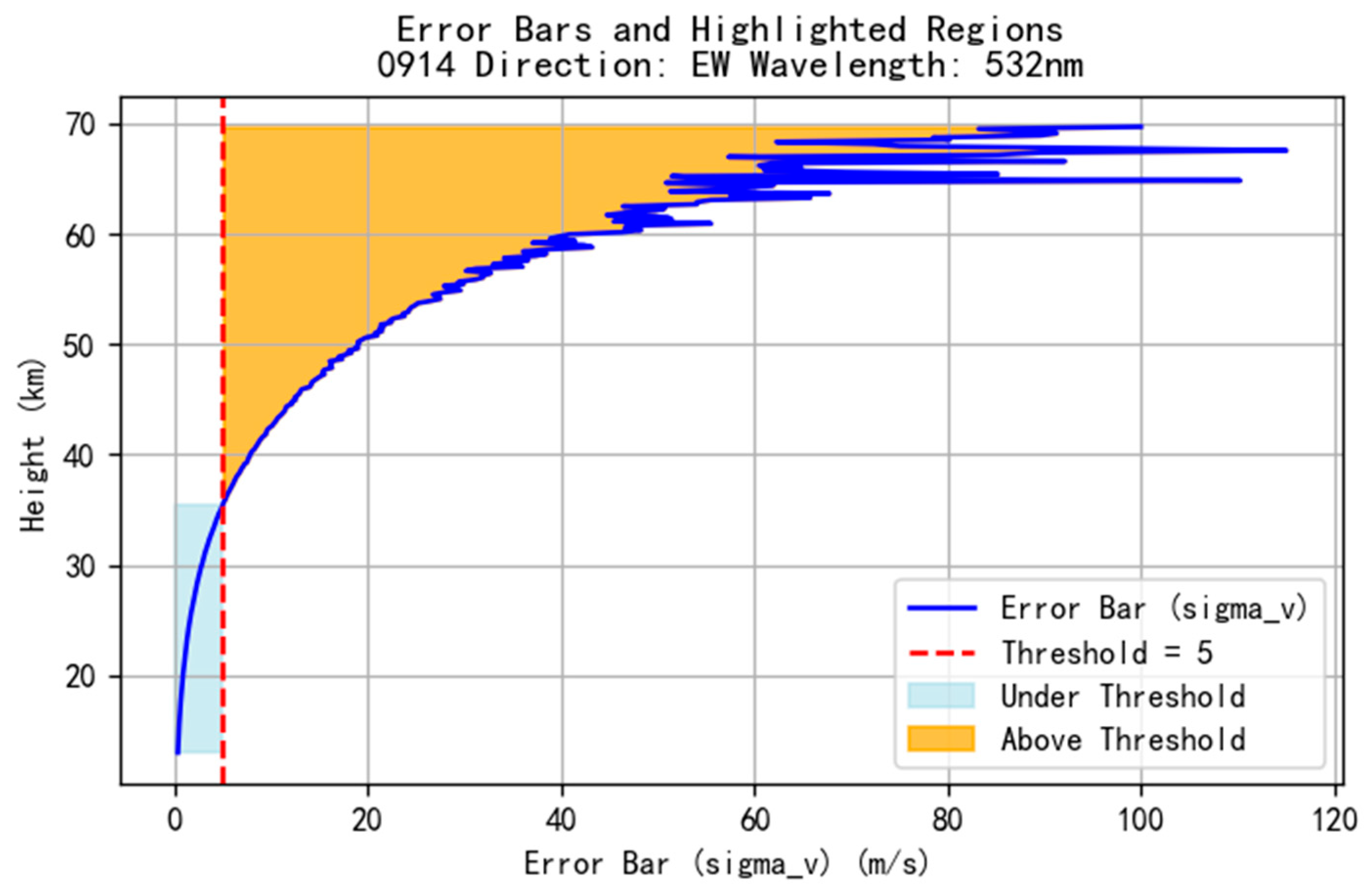
A more subtle E1 case reflects the mismatch between LLM interpretation and human intuition in user intents. For the request illustrated in Appendix A.2.2, “highlight altitude regions where the error bar exceeds a threshold for date 0914 EW,” the agent returned an error-bar-centered plot with the relevant regions highlighted correctly. However, a human evaluator instead expected a wind-profile-centered visualization. It suggests that even when the LLM correctly captures the explicit numerical condition in a request, it may still differ from a human user in identifying the most intuitive expected form of presentation. More broadly, this points to a limitation in aligning LLM interpretation with the subtext or the implicit reference often embedded in human language.

These representative cases show that the remaining limitations of the framework arise at multiple levels of the agent pipeline. However, in a constrained scientific workflow of this kind, many potential improvements are not simply additive. Their inclusion must be weighed against practical trade-offs among robustness, latency, and controllability. Under the current setting, the present design reflects what we regard as a reasonable balance. At the same time, the framework is still partly limited by the capabilities of the underlying LLM. As stronger base models become available, both result quality and task success rates may improve further without requiring fundamental changes to the agent architecture itself.

4. Discussion

A key source of the framework’s execution reliability is the separation between the fixed domain-specific tools and the LLM-based orchestration layer. In the present design, trusted scientific tools remain responsible for numerical processing, whereas the LLM primarily handles workflow planning, textual response generation, and new tool creation when required. This separation reduces the risk of groundless LLM hallucination at the level of core scientific computation and helps preserve reproducibility, because the same processing routine can be re-executed under the same tool definitions and inputs. The shared state, which serves as the memory module, further supports iterative analysis by storing and reusing intermediate products across turns, thereby reducing redundant computation and improving the stability of multi-turn interactions. In addition, validation and repair mechanisms constrain open-ended generation by checking artifact types, execution preconditions, and numerical plausibility, and by providing targeted feedback when failures occur.

Beyond data analysis, the framework also suggests a pathway toward more autonomous LiDAR operation for future deployment. The agent can invoke tools corresponding to instrument-control functions, including basic mechanical and system-level operations such as power cycling, angular rotation, laser-frequency stabilization, and optical-path switching. In this way, the architecture defines a unified software control layer between high-level decision logic and low-level device drivers. Although these control tools are currently implemented only as demonstrations and have not yet been deployed on physical hardware, formalizing control interfaces as callable tools is an important architectural step, as it allows decision logic to be developed, tested, and validated independently of full hardware integration. This design further enables data-guided automation, in which intermediate analysis products can serve as control signals. For example, the agent could detect systematic deviations in retrieved wind profiles caused by laser-frequency drift and trigger an updated stabilizer configuration to mitigate zero-Doppler bias. However, true closed-loop autonomous control would require additional safety constraints, timing guarantees, and conservative fallback policies, and remains a significant engineering challenge.

The same tool-oriented paradigm can also support knowledge-assisted interpretation. In the current implementation, this capability is demonstrated through a local database rather than live web sources. Although this limits time-sensitive contextualization, it establishes a practical pattern in which external references—such as campaign logs, instrument manuals, reanalysis summaries, or meteorological bulletins—are exposed as documentation or structured data. These knowledge sources can then be queried, checked, and integrated with numerical outputs under the same validation and provenance framework. This provides a principled way to combine computational results with contextual evidence without reducing the transparency of the overall analysis process.

Although the fusion criteria, detailed in Section 2.5.3, reduce inconsistencies among data sources, theoretical bias amplification remains a potential risk when an LLM is used to summarize geospatial wind products. The framework standardizes units, coordinates, and collocation procedures before comparison, and the prompts instruct the agent to treat low-SNR regions and large-error-bar regions cautiously. However, the textual summary generated by the LLM can still contain residual hallucination or overinterpretation, especially when LiDAR retrievals are noisy. Therefore, the agent-generated interpretation should be understood as an assisted summary grounded in computed products rather than as an independent theoretical judgment.

Despite these strengths, the present framework still operates within a bounded scope. Its performance currently depends on curated pre-processed databases and is strongest when user requests can be mapped onto supported analytical intents and validated workflow patterns. More open-ended requests, longer analysis chains, and workflows involving newly generated tool components remain comparatively challenging, partly because the batch evaluation setting is limited to single-turn interactions. Future improvements should focus on expanding intent coverage, strengthening workflow constraints, further hardening dynamically generated tools through systematic testing, tightening numerical validation, and introducing multimodal inspection for visualization outputs.

Looking forward, three directions appear particularly important. First, connecting the control layer to real LiDAR hardware and linking the knowledge layer to live meteorological databases and online information sources would enable more complete end-to-end automation. It would also allow the framework to be validated under real operating conditions, including tasks such as raw-data selection, altitude-coverage monitoring, cloud-aware scanning adjustment, and stabilizer tuning under laser-frequency drift. Second, equipping the system with an offline planning capability through a compact local LLM—for example, a LoRA-adapted model of approximately 7 billion parameters—could improve deployability in field campaigns with limited connectivity, while also benefiting data privacy and system independence. In our current prototype, a local LLM (qwen2.5-coder: 7b) has already been integrated for intent detection and workflow planning through Ollama, but it does not yet provide sufficient reliability for validation and dynamic tool creation. Thus, we did not include it in the result evaluation. Finally, the preliminary transfer example to CDL in Section 3.2.3 suggests that the architecture is not intrinsically tied to a single retrieval chain or data format. Since the workflow planning and tool generation can be conditioned by instrument-specific guidance, the same agent framework can in principle be adapted across wind LiDAR modalities by supplying only the corresponding documentation and data. This suggests a broader portability beyond simple dataset transfer, with the potential to extend the framework to a wide range of scientific instruments whose workflows depend on modular numerical procedures, provided that appropriate domain knowledge and procedural guidance are available. This portability makes the framework particularly useful for LiDAR researchers, remote-sensing instrument teams, and geospatial analysts who require reproducible, stateful, and tool-based processing of complex instrument data.

5. Conclusions

We have presented the ICDL-Agent, a tool-augmented LLM framework for remote sensing instrument workflows in Incoherent Doppler LiDAR analysis. By combining trusted domain-specific tools with structured planning, validation, and bounded repair, the framework translates natural-language analytical requests into executable and inspectable workflows for wind retrieval, uncertainty estimation, visualization, and higher-level diagnostics. Using atmospheric wind LiDARs as case studies, the results show that constrained LLM orchestration can support transparent and reproducible workflow automation for remote sensing instruments while reducing reliance on hand-written scripting and manual workflow coordination. The study also indicates that the framework can extend beyond a single fixed retrieval chain through controlled tool generation and preliminary transfer to other remote sensing instruments. More broadly, this work demonstrates the potential of LLM-based workflow systems for analyzing geospatial environmental observations, especially in settings where scientific traceability, intermediate-state management, and physically grounded computation must remain central. Future work will focus on integrating live instrument-control interfaces, improving robustness in tool-creation scenarios, and extending the framework to real-time analysis and broader classes of atmospheric observations.

References

1. Chanin, M.L.; Garnier, A.; Hauchecorne, A.; Porteneuve, J. A Doppler lidar for measuring winds in the middle atmosphere. Geophys. Res. Lett. 1989, 16, 1273–1276. [Google Scholar] [CrossRef]
2. Chanin, M.; Hauchecorne, A. Lidar observation of gravity and tidal waves in the stratosphere and mesosphere. J. Geophys. Res. Oceans 1981, 86, 9715–9721. [Google Scholar] [CrossRef]
3. Garnier, A.; Chanin, M.L. Description of a Doppler rayleigh LIDAR for measuring winds in the middle atmosphere. Appl. Phys. B 1992, 55, 35–40. [Google Scholar] [CrossRef]
4. Korb, C.L.; Gentry, B.M.; Weng, C.Y. Edge technique: Theory and application to the lidar measurement of atmospheric wind. Appl. Opt. 1992, 31, 4202–4213. [Google Scholar] [CrossRef]
5. Flesia, C.; Korb, C.L. Theory of the double-edge molecular technique for Doppler lidar wind measurement. Appl. Opt. 1999, 38, 432–440. [Google Scholar] [CrossRef] [PubMed]
6. Baumgarten, G. Doppler Rayleigh/Mie/Raman lidar for wind and temperature measurements in the middle atmosphere up to 80 km. Atmos. Meas. Tech. 2010, 3, 1509–1518. [Google Scholar] [CrossRef]
7. Gardner, C.S.; Miller, M.S.; Liu, C.-H. Rayleigh lidar observations of gravity wave activity in the upper stratosphere at Urbana, Illinois. J. Atmos. Sci. 1989, 46, 1838–1854. [Google Scholar] [CrossRef]
8. Dou, X.; Han, Y.; Sun, D.; Xia, H.; Shu, Z.; Zhao, R.; Shangguan, M.; Guo, J. Mobile Rayleigh Doppler lidar for wind and temperature measurements in the stratosphere and lower mesosphere. Opt. Express 2014, 22, A1203–A1221. [Google Scholar] [CrossRef]
9. Zhao, R.-C.; Xia, H.-Y.; Dou, X.-K.; Sun, D.-S.; Han, Y.-L.; Shangguan, M.-J.; Guo, J.; Shu, Z.-F. Correction of temperature influence on the wind retrieval from a mobile Rayleigh Doppler lidar. Chin. Phys. B 2015, 24, 024218. [Google Scholar] [CrossRef][Green Version]
10. Chen, C.; Xue, X.; Sun, D.; Zhao, R.; Han, Y.; Chen, T.; Liu, H.; Zhao, Y. Comparison of Lower Stratosphere Wind Observations From the USTC’s Rayleigh Doppler Lidar and the ESA’s Satellite Mission Aeolus. Earth Space Sci. 2022, 9, e2021EA002176. [Google Scholar] [CrossRef]
11. Yamashita, C.; Chu, X.; Liu, H.L.; Espy, P.J.; Nott, G.J.; Huang, W. Stratospheric gravity wave characteristics and seasonal variations observed by lidar at the South Pole and Rothera, Antarctica. J. Geophys. Res. Atmos. 2009, 114, D12101. [Google Scholar] [CrossRef]
12. Sun, D.; Zhong, Z.; Zhou, J.; Hu, H.; Kobayashi, T. Accuracy Analysis of the Fabry–Perot Etalon Based Doppler Wind Lidar. Opt. Rev. 2005, 12, 409–414. [Google Scholar] [CrossRef]
13. Zhang, N.; Sun, D.; Han, Y.; Chen, C.; Wang, Y.; Zheng, J.; Liu, H.; Han, F.; Zhou, A.; Tang, L. Zero Doppler correction for Fabry–Pérot interferometer-based direct-detection Doppler wind LIDAR. Opt. Eng. 2019, 58, 054101. [Google Scholar] [CrossRef]
14. Vaswani, A.; Shazeer, N.; Parmar, N.; Uszkoreit, J.; Jones, L.; Gomez, A.N.; Kaiser, L.; Polosukhin, I. Attention is all you need. In Proceedings of the Advances in Neural Information Processing Systems, Long Beach, CA, USA, 4–9 December 2017. [Google Scholar]
15. Brown, T.; Mann, B.; Ryder, N.; Subbiah, M.; Kaplan, J.D.; Dhariwal, P.; Neelakantan, A.; Shyam, P.; Sastry, G.; Askell, A.; et al. Language Models are Few-Shot Learners. In Proceedings of the Advances in Neural Information Processing Systems; Curran Associates: Red Hook, NY, USA, 2020; pp. 1877–1901. [Google Scholar]
16. Beurer-Kellner, L.; Fischer, M.; Vechev, M. Prompting Is Programming: A Query Language for Large Language Models. Proc. ACM Program. Lang. 2023, 7, 1946–1969. [Google Scholar] [CrossRef]
17. Vemprala, S.H.; Bonatti, R.; Bucker, A.; Kapoor, A. ChatGPT for Robotics: Design Principles and Model Abilities. IEEE Access 2024, 12, 55682–55696. [Google Scholar] [CrossRef]
18. Schick, T.; Dwivedi-Yu, J.; Dessì, R.; Raileanu, R.; Lomeli, M.; Hambro, E.; Zettlemoyer, L.; Cancedda, N.; Scialom, T. Toolformer: Language Models Can Teach Themselves to Use Tools. In Proceedings of the Thirty-Seventh Conference on Neural Information Processing Systems, New Orleans, LA, USA, 10–16 December 2023. [Google Scholar]
19. Devlin, J.; Chang, M.-W.; Lee, K.; Toutanova, K. BERT: Pre-training of Deep Bidirectional Transformers for Language Understanding. arXiv 2018, arXiv:1810.04805. [Google Scholar]
20. Achiam, J.; Adler, S.; Agarwal, S.; Ahmad, L.; Akkaya, I.; Aleman, F.L.; Almeida, D.; Altenschmidt, J.; Altman, S.; Anadkat, S.; et al. GPT-4 Technical Report. arXiv 2023, arXiv:2303.08774. [Google Scholar]
21. Yao, S.; Zhao, J.; Yu, D.; Du, N.; Shafran, I.; Narasimhan, K.; Cao, Y. ReAct: Synergizing Reasoning and Acting in Language Models. arXiv 2023, arXiv:2210.03629. [Google Scholar] [CrossRef]
22. OpenAI. Introducing GPT-5. 2025. Available online: https://openai.com/index/introducing-gpt-5/ (accessed on 20 March 2026).
23. Zhang, Y.; Li, J.; Wang, Z.; He, Z.; Guan, Q.; Lin, J.; Yu, W. Geospatial large language model trained with a simulated environment for generating tool-use chains autonomously. Int. J. Appl. Earth Obs. Geoinf. 2025, 136, 104312. [Google Scholar] [CrossRef]
24. Pierdicca, R.; Muralikrishna, N.; Tonetto, F.; Ghianda, A. On the Use of LLMs for GIS-Based Spatial Analysis. ISPRS Int. J. Geo-Inf. 2025, 14, 401. [Google Scholar] [CrossRef]
25. Zhan, Y.; Xiong, Z.; Yuan, Y. SkyEyeGPT: Unifying remote sensing vision-language tasks via instruction tuning with large language model. ISPRS J. Photogramm. Remote Sens. 2025, 221, 64–77. [Google Scholar] [CrossRef]
26. Bran, A.M.; Cox, S.; Schilter, O.; Baldassari, C.; White, A.D.; Schwaller, P. ChemCrow: Augmenting Large-Language Models with Chemistry Tools. Nat. Mach. Intell. 2024, 6, 525–535. [Google Scholar] [CrossRef] [PubMed]
27. Nie, Y.; Gao, S. ChatGPT for Intelligent Spatial Analysis Workflow Construction. In SIGSPATIAL ‘24: Proceedings of the 32nd ACM International Conference on Advances in Geographic Information Systems; Association for Computing Machinery: New York, NY, USA, 2024. [Google Scholar]
28. Xi, Z.; Chen, W.; Guo, X.; He, W.; Ding, Y.; Hong, B.; Zhang, M.; Wang, J.; Jin, S.; Zhou, E.; et al. The rise and potential of large language model based agents: A survey. Sci. China Inf. Sci. 2025, 68, 121101. [Google Scholar] [CrossRef]
29. Luo, Q.; Lin, Q.; Xu, L.; Wu, S.; Mao, R.; Wang, C.; Feng, H.; Huang, B.; Du, Z. GeoJSON agents: A multi-agent LLM architecture for geospatial analysis—Function calling vs. code generation. Big Earth Data 2026, 1–55. [Google Scholar] [CrossRef]
30. Xing, Z.; Meng, Z.; Zheng, G.; Yang, L.; Guo, X.; Tan, L.; Jiang, Y. Human-computer interactive rehabilitation: A 3D graph deep learning method for non-contact gesture recognition in post-epidemic and aging societies. Measurement 2026, 257, 118794. [Google Scholar] [CrossRef]
31. Xing, Z.; Li, L.; Yang, Y.; Zhou, W.; Ma, G.; Chen, S.; Lyu, L.; Li, X. A lightweight model for indoor object detection in unstructured scenes based on joint attention and prior knowledge in the context of home rehabilitation. J. King Saud Univ. Comput. Inf. Sci. 2026. [Google Scholar] [CrossRef]
32. Li, J.; Chen, C.; Han, Y.; Chen, T.; Xue, X.; Liu, H.; Zhang, S.; Yang, J.; Sun, D. Wind Profile Reconstruction Based on Convolutional Neural Network for Incoherent Doppler Wind LiDAR. Remote Sens. 2024, 16, 1473. [Google Scholar] [CrossRef]
33. Song, Y.; Han, Y.; Su, Z.; Chen, C.; Sun, D.; Chen, T.; Xue, X. Denoising coherent Doppler lidar data based on a U-Net convolutional neural network. Appl. Opt. 2024, 63, 275–282. [Google Scholar] [CrossRef]
34. Kliebisch, O.; Uittenbosch, H.; Thurn, J.; Mahnke, P. Coherent Doppler wind lidar with real-time wind processing and low signal-to-noise ratio reconstruction based on a convolutional neural network. Opt. Express 2022, 30, 5540–5552. [Google Scholar] [CrossRef]
35. Mohandes, M.A.; Rehman, S. Wind Speed Extrapolation Using Machine Learning Methods and LiDAR Measurements. IEEE Access 2018, 6, 77634–77642. [Google Scholar] [CrossRef]
36. Han, Y.; Sun, D.; Han, F.; Liu, H.; Zhao, R.; Zhen, J.; Zhang, N.; Chen, C.; Li, Z. Demonstration of daytime wind measurement by using mobile Rayleigh Doppler Lidar incorporating cascaded Fabry-Perot etalons. Opt. Express 2019, 27, 34230–34246. [Google Scholar] [CrossRef] [PubMed]
37. Craven, G.W.P. Smoothing noisy data with spline functions. Numer. Math. 1978, 31, 377–403. [Google Scholar] [CrossRef]
38. Weinert, H.L. Efficient computation for Whittaker–Henderson smoothing. Comput. Stat. Data Anal. 2007, 52, 959–974. [Google Scholar] [CrossRef]
39. Eilers, P.H. A Perfect Smoother. Anal. Chem. 2003, 75, 3631–3636. [Google Scholar] [CrossRef]
40. Chen, C.; Zhang, N. Wind observations of USTC Rayleigh Doppler Lidar in 2019 (Xinjiang); Science Data Bank: Beijing, China, 2022. [Google Scholar]
41. Kong, S.Z.A.; Chen, H.; Li, Q.; Qin, Y.; Sun, R.; Zhou, X.; Wang, E.; Dong, X. Better Zero-Shot Reasoning with Role-Play Prompting. In Proceedings of the 2024 Conference of the North American Chapter of the Association for Computational Linguistics: Human Language Technologies, Mexico City, Mexico, 16–21 June 2024; Gomez, H., Duh, K., Bethard, S., Eds.; Association for Computational Linguistics: Stroudsburg, PA, USA, 2024; Volume 1, pp. 4099–4113. [Google Scholar] [CrossRef]
42. White, Q.F.J.; Hays, S.; Sandborn, M.; Olea, C.; Gilbert, H.; Elnashar, A.; Spencer-Smith, J.; Schmidt, D.C. A Prompt Pattern Catalog to Enhance Prompt Engineering with ChatGPT. In Proceedings of the 30th Conference on Pattern Languages of Programs, Monticello, IL, USA, 23–25 October 2023. [Google Scholar]
43. Gao, A.M.L.; Zhou, S.; Alon, U.; Liu, P.; Yang, Y.; Callan, J.; Neubig, G. PAL: Program-aided language models. In Proceedings of the 40th International Conference on Machine Learning, Honolulu, HI, USA, 23–25 October 2023. [Google Scholar]
Figure 1. Overview of the ICDL-Agent architecture. Solid arrows indicate the input workflow, while dashed arrows indicate intermediate data flow.
Ijgi 15 00238 g001
Figure 2. Simulated Rayleigh Backscattered Signal and the Fitted Transmission Curve.
Ijgi 15 00238 g002
Figure 3. Plot of the Refined Response Curve.
Ijgi 15 00238 g003
Figure 4. Overall architecture of the LiDAR agent, showing the logical nodes, shared agent state, and tool registry. Purple blocks denote logical nodes and the tool registry; yellow blocks denote data storage modules; gray blocks denote agent inputs and outputs; and the green block indicates the decision-branch node. Purple arrows indicate the main workflow; green arrows indicate positive-decision workflow branches; red arrows indicate negative-decision workflow branches; and gray arrows indicate data flow. The LiDAR hardware and online database modules (shown without background color) are planned for future integration.
Ijgi 15 00238 g004
Figure 5. Simplified Agent Workflow.
Ijgi 15 00238 g005
Figure 6. Workflow With Tool Creation.
Ijgi 15 00238 g006
Figure 7. Representative Visualizations Generated by the Agent: (a) FPI Transmission Curve Fitting; (b) Retrieved Wind Profile; (c) Retrieved Wind Field; (d) Gravity Wave 2D Fast-Fourier-Transformation (FFT) Spectrum of Wind Field.
Ijgi 15 00238 g007
Figure 8. Representative comparisons of retrieved wind profiles from the traditional algorithm, the agent-assisted algorithm, and external reference data.
Ijgi 15 00238 g008
Figure 9. Representative Case of Interactive Analysis Case.
Ijgi 15 00238 g009
Figure 10. (a) Wavelet Power Spectrum of the EW wind field on 22 October. The small red dots denote the local maxima of the wavelet transformation power spectrum. (b) 2D FFT Spectrum For gravity Wave Analysis of EW Wind Field on 22 October. The red circle indicates the peak-power point of the FFT power spectrum.
Ijgi 15 00238 g010
Figure 11. Intensity Profile and Wind Profile Generated for CDL in Hefei, China on 9 February 2025: (a) Signal Intensity Profile of the CDL; (b) The Retrieved Wind Profile of the CDL.
Ijgi 15 00238 g011