Article

Comparative Analysis of Machine Learning–Kriging Integrative Approaches for Enhanced Spatial Prediction of Mineral Exploration Data

1
Department of Energy and Mineral Resources Engineering, Kangwon National University, Samcheok-si 25913, Republic of Korea
2
Exploration & Mining Research Team, Korea Mine Rehabilitation and Mineral Resources Corporation, Wonju-si 26464, Republic of Korea
3
Department of Green Energy Engineering, Kangwon National University, Samcheok-si 25913, Republic of Korea
*
Author to whom correspondence should be addressed.
ISPRS Int. J. Geo-Inf. 2026, 15(4), 175; https://doi.org/10.3390/ijgi15040175
Submission received: 15 February 2026 / Revised: 5 April 2026 / Accepted: 12 April 2026 / Published: 15 April 2026
(This article belongs to the Topic Geospatial AI: Systems, Model, Methods, and Applications)

Abstract

Accurate prediction of mineral concentrations from sparse exploration data is important for resource estimation. This study evaluates hybrid prediction models combining machine learning (ML) and geostatistics to predict aluminum (Al) concentrations. Twelve hybrid configurations were generated by combining six ML backbones—Random Forest, XGBoost, AdaBoost, ResNet, U-Net, and Spatial Transformer Network—with Ordinary Kriging (OK) and Universal Kriging (UK). Model performance was evaluated using 10-fold spatial cross-validation (CV) to reduce spatial leakage, and hyperparameters were tuned by grid-search CV within the training folds. For the hybrid models, residual kriging was fitted using cross-fitted out-of-fold residuals to reduce optimistic bias and prevent information leakage. The results showed no consistent performance separation between OK and UK variants. More importantly, the effect of integration was backbone dependent rather than uniformly beneficial. RF-based predictions showed the strongest overall out-of-sample performance, whereas hybrid gains for other backbones were generally modest. After multiple-comparison correction, most differences between standalone and hybrid models were not statistically significant. These findings indicate that increasing model complexity through hybridization does not guarantee improved accuracy and highlight the importance of spatially explicit, bias-aware evaluation when selecting prediction strategies for mineral resource exploration.

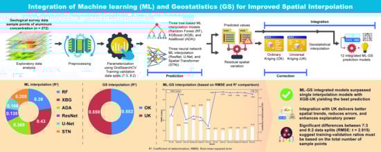
Graphical Abstract

1. Introduction

In mineral resource exploration, geological investigation data are essential for evaluating the resource value and development feasibility. These data, typically collected at discrete locations, often suffer from limited and uneven sampling owing to spatial and physical constraints [1]. Although geostatistical (GS) methods have traditionally been used to estimate values at unsampled locations, their performance may be limited in settings with strong spatial heterogeneity, nonlinear relationships, and outliers [2,3,4,5,6]. In particular, while GS methods are effective for modeling spatial dependence, they may be less suited to representing complex nonlinear relationships among multiple predictors.
To address these limitations, methods such as co-kriging, spatial regression, and Bayesian approaches have been developed to represent global trends and local variability by incorporating auxiliary variables and spatial information. Co-kriging combines sparse and high-density data to mitigate sampling limitations; spatial regression augments kriging with explanatory variables; and Bayesian methods can improve uncertainty characterization by accounting for parameter uncertainty. In contrast, machine learning (ML) approaches, which have recently gained prominence, excel at detecting complex nonlinear patterns but may underutilize spatial dependence if spatial structure is not explicitly modeled [7]. Thus, integrating ML and GS methods can combine nonlinear pattern learning from ML with spatial interpolation and uncertainty characterization from GS, potentially improving prediction performance when residual spatial structure remains after the trend component is modeled.
Recent studies have combined ML and GS methods for spatial prediction, as summarized in Table 1. According to recent reviews [8,9], these hybrid approaches can be broadly categorized into two primary strategies. The first is ‘feature space enhancement (FSE),’ where GS outputs (e.g., kriging estimates) and/or spatial coordinates are used as additional predictors for ML models. The second strategy, often referred to as regression kriging (RK), is a two-step procedure in which an ML model predicts the deterministic component and GS interpolation is subsequently applied to the model residuals. Under our selection criteria, explicit examples of the FSE strategy were comparatively limited, whereas most selected studies adopted an RK workflow in which an ML model captures the deterministic component and GS interpolation is applied to the residuals. Accordingly, Table 1 focuses on representative RK-type hybrid models. Although various ML models, such as artificial neural networks [10], extreme learning machines [11], and support vector regression [12] have been employed in hybrid studies, random forest (RF) has been one of the most frequently used learners in RK-type applications [13,14,15,16,17]. Among the GS methods, ordinary kriging (OK) has been predominantly used for residual interpolation, although co-kriging and empirical Bayesian kriging have also been considered in some studies. In this study, we adopt an RK framework to combine ML models for learning complex, nonlinear relationships between auxiliary variables and mineral concentrations with GS methods (OK and universal kriging, UK) for modeling the remaining spatial autocorrelation in the residuals. Although such hybrid ML–GS approaches have been widely applied in environmental applications (e.g., soil organic matter and biomass prediction), their application to mineral resource exploration remains comparatively limited. Moreover, direct head-to-head comparisons across multiple ML backbones and kriging variants under a unified spatial validation design are still scarce. Accordingly, this study presents a case-specific comparative evaluation of ML architectures coupled with two kriging strategies within an RK framework.
This study evaluates whether integrating tree-based and neural network (NN)-based ML models with GS methods (OK and UK) improves out-of-sample prediction of aluminum (Al) concentrations under spatially explicit validation. The primary objective is to compare the extent to which hybrid RK models provide incremental prediction benefit relative to standalone ML and GS models under a validation design that reduces spatial dependence between training and test folds. In addition, this analysis is restricted to spatial prediction at a single time point and a single case-study dataset; therefore, the findings should be interpreted as case specific rather than as fully general conclusions.

2. Materials and Methods

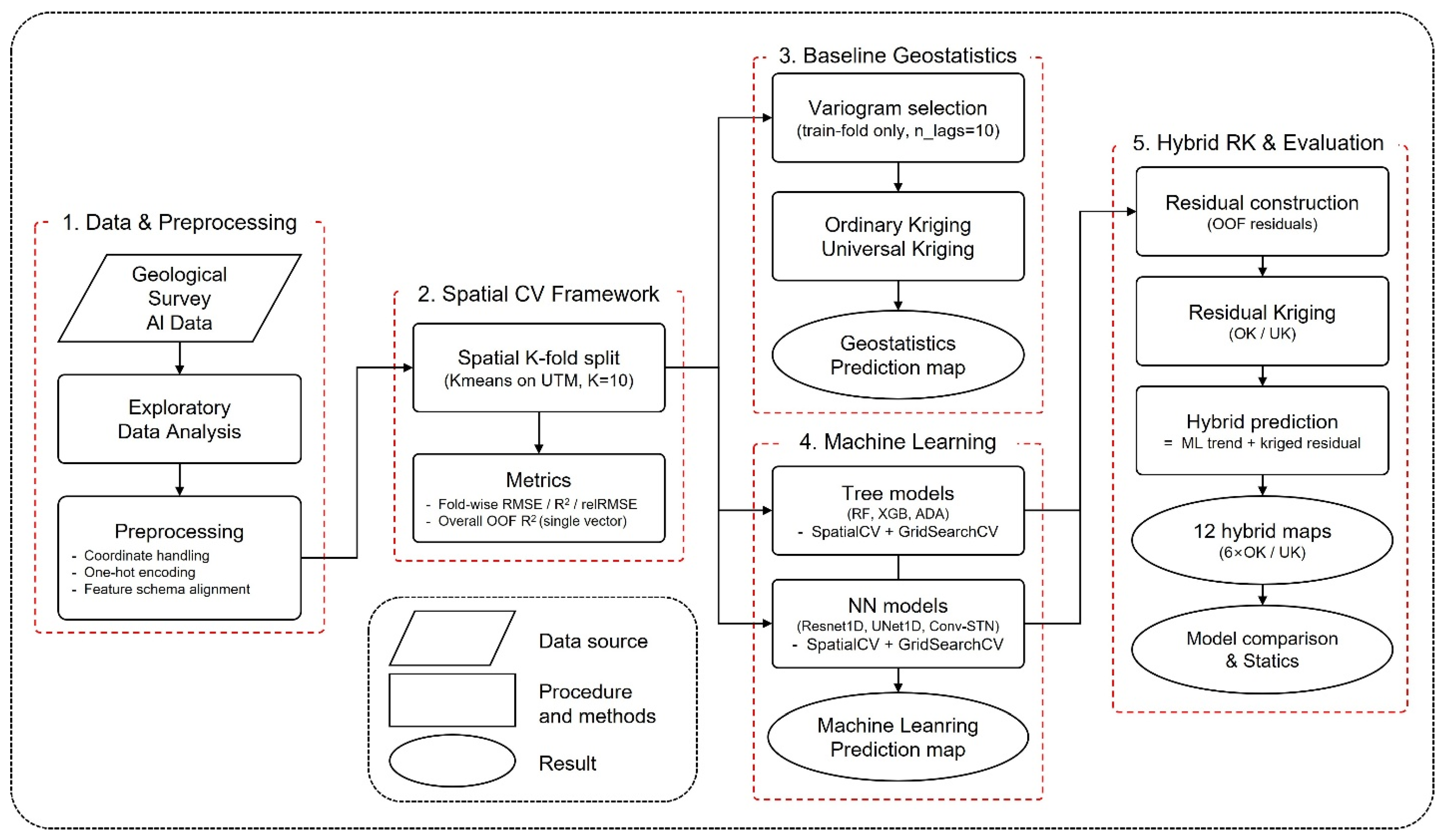
Figure 1 summarizes the study workflow in five modules: (1) exploratory data analysis (EDA) and preprocessing; (2) construction of a spatial cross-validation (CV) framework and definition of the evaluation metrics; (3) baseline GS interpolation (OK and UK) with variogram modeling performed using the training fold only; (4) development and hyperparameter tuning of ML models within each training spatial fold; and (5) hybrid RK, in which the ML model first predicts the trend component and kriging is then fitted to residuals derived exclusively from the training data, using within-training CV to generate out-of-fold (OOF) residuals, before the kriged residuals are added to the ML trend. In the spatial CV framework, the held-out fold was reserved only for final performance assessment and was not used for variogram modeling, ML tuning, or residual kriging, thereby preventing information leakage. Visualization was performed using ArcGIS Pro 3.6, and all computations were conducted in Python 3.12.12 with scikit-learn, PyTorch 2.9.1 (CUDA 12.8; cuDNN 9.10.02), and PyKrige V1.7.2 [18].

2.1. Study Area and Dataset

The study area is located near Samcheok and Taebaek in Gangwon State, Republic of Korea, within the Taebaek Mountain Range. Geologically, the study area includes the Myeonsan Formation, which has been described as part of the Early Cambrian succession in the Taebaek area. The area comprises diverse lithologies and surficial materials distributed across the regional geological framework, and the region historically hosted metal, nonmetal, and coal mines, although most are now inactive owing to limited economic viability. The Korea Institute of Geoscience and Mineral Resources [19] has identified a titanium (Ti)-bearing mineralized zone in the Myeonsan Formation with an average grade of 6.95–9.1 wt.% TiO2 and inferred resources of 85.1 million tons, and exploration is ongoing in this area. Previous mineralogical characterization [20] indicates that this Ti occurs mainly as rutile and iron mainly as hematite, with quartz as the dominant gangue mineral and minor muscovite also present. Optical microscopy and mineralogical observation further suggest that the ore is hosted by sedimentary rocks (mudstone and sandstone), in which quartz occurs as relatively discrete grains while clay minerals surround fine intergrowths of hematite and rutile. In this study, Al was selected as the target variable because it is geochemically relevant to the Ti-bearing mineralization and is also of industrial interest.
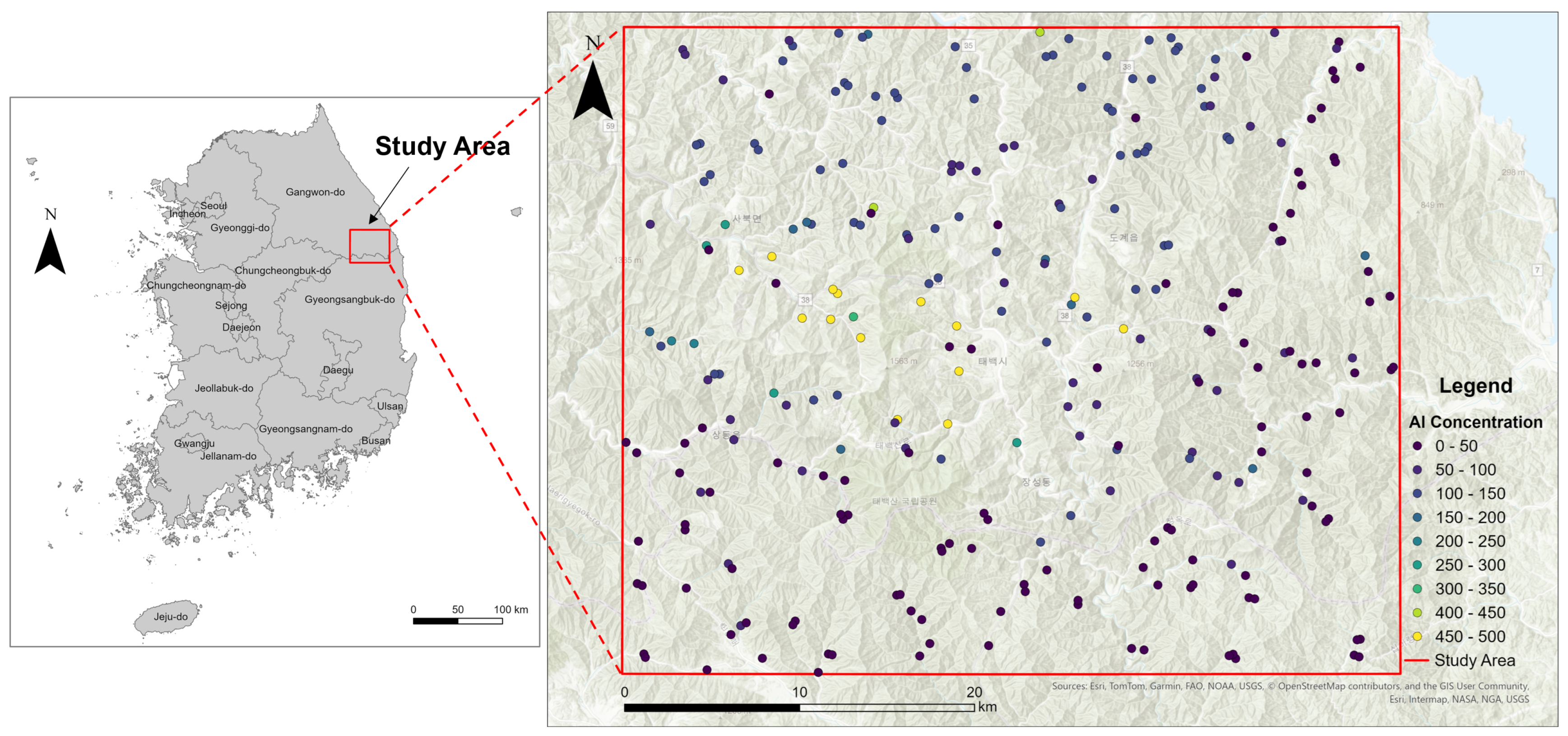
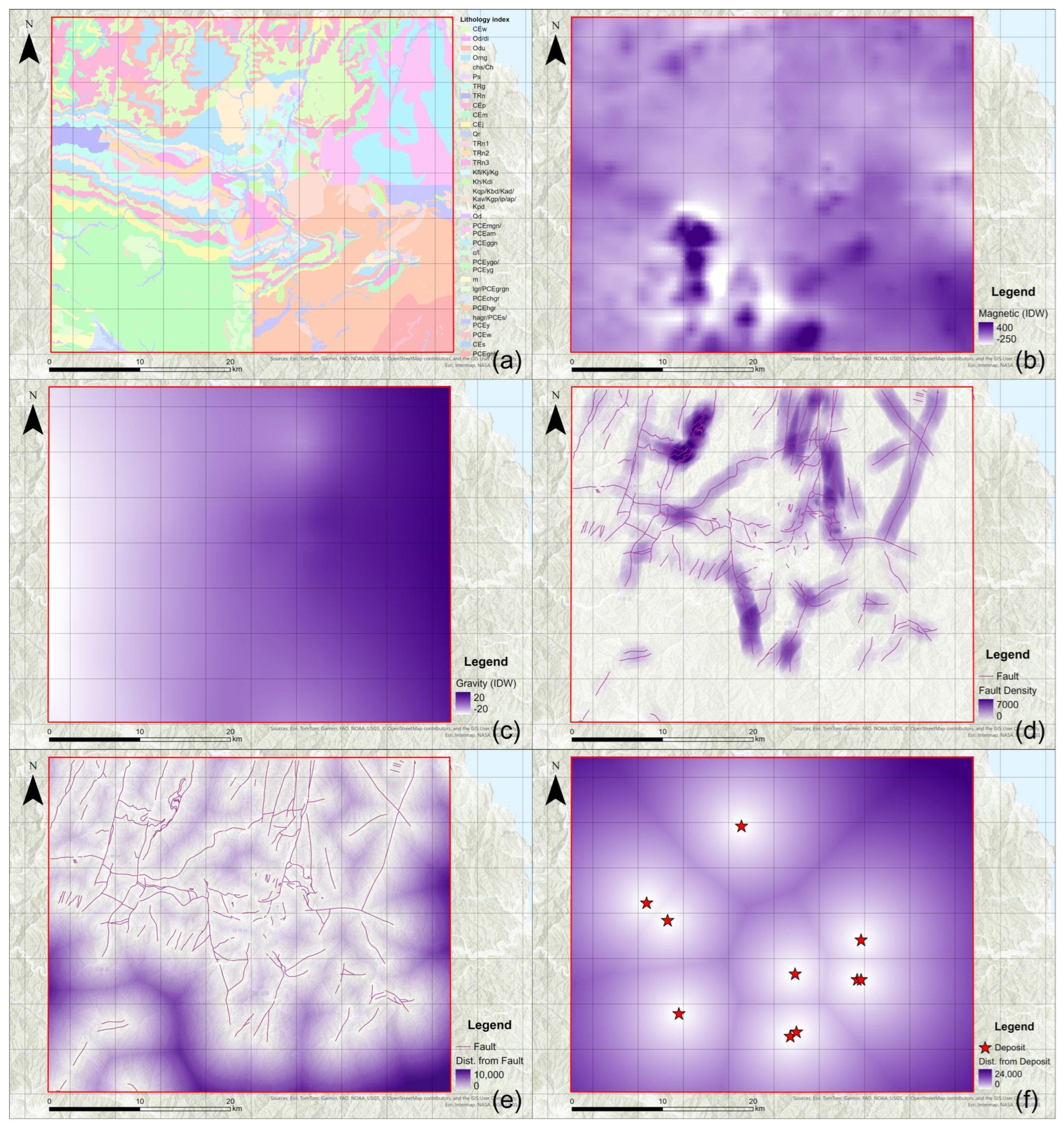
Figure 2 shows the distribution of 272 Al concentrations measurements (mg/kg) collected from surface survey samples in the study area; underground samples were not included. The samples are distributed between 37°00′13.72″ and 37°20′01.83″ N and 128°44′59.31″ and 129°14′37.24″ E. High Al concentrations, including several outliers, were mainly observed in the midwestern part of the study area, whereas most other sites showed relatively low values. Figure 3 presents the auxiliary variables used for spatial prediction across the study area: grouped lithologic classes, magnetic anomaly [21], gravity anomaly [22], fault density, distance from faults, and distance from deposits [23]. The multicolored polygons in Figure 3a represent grouped lithologic classes used as a categorical predictor for modeling Al concentrations. In addition to lithologic class, we used five covariates—magnetic anomaly, gravity anomaly, fault density, distance from faults, and distance from deposits—to explore geological controls on Al concentrations. To reduce sparsity in the lithologic categories and minimize inconsistencies between training and test data, the original 47 lithologic units were grouped into 30 broader lithologic classes based on geological similarity. We then confirmed that all grouped classes were represented in the data used for model development and evaluation.
Before preprocessing, we performed EDA to characterize the distribution of the raw data. Histograms and summary statistics were used to analyze the distribution of the target variable and the potential presence of outliers. We also computed an experimental semivariogram of raw Al concentrations to examine the presence of spatial autocorrelation in the original data. This semivariogram was used only for exploratory characterization; the variograms used for OK/UK modeling were selected and fitted separately within the training folds of the spatial CV procedure.

2.2. Integrated ML–GS Prediction Model

Because the sample size was relatively small (n = 272) and the data included potential outliers, model generalization was not assessed using a single random hold-out split. Instead, prediction performance was evaluated using spatial k-fold CV, which is better suited to geographically structured data and reduces the risk of overly optimistic estimates caused by spatial dependence between training and test samples. This framework provides a more stable basis for performance comparison and allows uncertainty in model performance to be summarized across folds. Model performance was reported using the mean and standard deviation of fold-wise errors, together with overall OOF predictions aggregated across all folds.

2.2.1. ML Prediction Model

To predict the spatial distribution of Al concentrations, we evaluated multiple ML algorithms using two-dimensional location information (latitude and longitude, mapped to Universal Transverse Mercator coordinates; UTM) together with six auxiliary predictors: grouped lithologic classes, magnetic anomaly, gravity anomaly, fault density, distance to faults, and distance to deposits. The evaluated ML models comprised (a) three tree-based ensemble regressors (random forest; RF, Extreme Gradient Boosting (XGBoost; XGB), and AdaBoost; ADA), and (b) three NN architectures (ResNet, U-Net, and a spatial transformer network; STN). The candidate hyperparameter settings used for model comparison are summarized in Table 2. For each outer spatial CV split, hyperparameters were optimized by grid-search CV using only the training portion of that split. In each outer spatial fold, models were trained on the training clusters and evaluated on the held-out cluster, which was reserved exclusively for out-of-sample performance evaluation. For readability, Table 2 reports simplified functional descriptions of some parameter settings (e.g., ‘all features’ rather than library-specific parameter labels such as ‘None’ in scikit-learn).
Tree-based ensemble models combine multiple decision trees to learn nonlinear relationships and predictor interactions. RF reduces variance by aggregating predictions from many decorrelated trees [24]. XGB builds trees sequentially by minimizing a gradient-based objective function [25]. ADA iteratively reweights training samples so that subsequent weak learners focus more on observations with larger prediction errors (i.e., larger residuals) [26].
NN-based models learn hierarchical feature representations through nonlinear transformations. ResNet uses residual connections that improve optimization stability in deeper architectures [27]. U-Net adopts an encoder-decoder structure with skip connections, enabling multiscale feature propagation [28]. STN incorporates a learnable geometric transformation module that can improve robustness to spatial distortions in the input representation [29].

2.2.2. GS Interpolation Method

Kriging is a widely used GS interpolation method for estimating values at unsampled locations on the basis of spatial autocorrelation characterized by a variogram [30,31]. In this study, we considered OK and UK, which differ in how the mean structure is represented: OK assumes a locally constant mean, whereas UK allows a deterministic trend component [32]. Both GS methods were evaluated within the same 10-fold spatial CV framework used for the ML models. For each outer fold, empirical variogram construction, model fitting, and kriging prediction were all based exclusively on the training data, whereas prediction performance was assessed only on the held-out fold to prevent information leakage.
To ensure consistency across folds, all empirical variograms were computed in the UTM projection using Euclidean distances, with the number of lags fixed at 10 and the same candidate model families (exponential, spherical, and Gaussian) considered in each fold. Candidate variogram models were evaluated using the scikit-gstat library, and the final variogram type and parameters were selected within each fold using the same criterion across folds (Table 3), namely the minimum fitting error (negative mean squared error) between the empirical semivariogram and the candidate theoretical model. The selected variogram model and its fitted parameters were then used for kriging prediction within the corresponding fold and for estimation of the kriging variance.
For UK, we used PyKrige’s Universal Kriging with coordinate-based drift terms (e.g., regional linear drift) so that the deterministic trend was represented as a function of spatial coordinates rather than auxiliary covariates. In this analysis, the auxiliary predictors were not included as drift terms in UK. Instead, they were used in the ML component, and the hybrid models incorporated them indirectly through the ML trend and subsequent residual kriging (Section 2.2.3).

2.2.3. Integrated ML–GS Model

ML models are effective for learning nonlinear relationships among the predictors, while GS models are effective for representing residual spatial autocorrelation and generating continuous prediction surfaces. Combining these two components can improve spatial prediction when the ML trend captures the deterministic structure and kriging accounts for remaining spatially structured errors [15].
In this study, we adopted an RK framework in which, within each outer spatial CV split, residual kriging was based exclusively on residuals derived from the training fold data. To reduce the optimistic bias that arises when residuals are computed in-sample, the training fold residuals were obtained by within-training CV (i.e., cross-fitted or OOF residuals), and these bias-reduced residuals were then used for variogram fitting and kriging. The RK workflow consisted of the following three steps:
  • Trend prediction: In each outer fold, the deterministic component was represented by the ML model selected and tuned as described in Section 2.2.1. The model was fitted using the training folds only, and predictions were generated for the held-out fold and for spatial mapping over the study area.
  • Residual modeling and kriging: An empirical variogram was constructed from the cross-fitted training residuals and fitted using the same variogram-selection procedure described in Section 2.2.2. The resulting OK or UK model was then used to predict the residual component for the held-out fold and to generate the residual surface over the study area.
  • Integration: Final predictions were obtained by adding the kriged residual surface to the ML trend prediction, thereby combining nonlinear trend learning from ML with spatial error correction from GS.
The cross-fitted ML residual at training location x i was defined as,
ε ^ M L x i = C x i Z ^ M L O O F ( x i ) ,
where C x i is the observed Al concentrations at location x i and Z ^ M L O O F ( x i ) is the OOF ML prediction obtained under within-training CV. The RK prediction at training location x i was then computed as,
Z ^ M L G S x = Z ^ M L x + R ^ G S x ,
where Z ^ M L x i denotes the ML trend prediction and R ^ G S x denotes the kriged residual surface fitted from the cross-fitted training residuals using OK or UK. This CV-based residual definition provides a consistent bias-reduced residual estimation strategy across all ML backbones, including models for which out-of-sample residuals are not available.

2.3. Performance Metrics and Spatial Cross-Validation Assessment

To reduce bias arising from spatial autocorrelation, all modeling approaches (ML, GS, and Integrated ML-GS models) were trained and evaluated using a 10-fold spatial CV framework rather than simple random split. In each split, the held-out fold was reserved exclusively for out-of-sample performance assessment, while model fitting was performed using the remaining folds. During hyperparameter optimization, model selection was based on the negative mean squared error score (i.e., scikit-learn’s neg_mean_squared_error), which is equivalent to minimizing the mean squared error (MSE). For final model comparison, RMSE (RMSE = √MSE), as presented in Equation (3), was treated as the primary performance metric:
R M S E   =   i   =   1 n ( y ^ i y i ) 2 n ,
where y ^ i , is the predicted value at point i , y i denotes the observed value, and n is the number of evaluated samples. RMSE was selected as the primary metric because it measures the magnitude of the prediction errors in the original unit of the target variable (mg/kg), which facilitates direct interpretation [33]. Lower RMSE values indicate better prediction accuracy.
As a supplementary scale-independent summary, we also report the relative RMSE (relRMSE), defined as RMSE divided by the mean of the observed values in the evaluation set. We additionally used predictive R2 as a second supplementary measurement of out-of-sample prediction skill:
R p r e d 2   =   1 S S E S S T ,   S S E   =   y i y ^ i 2 ,   S S T   =   ( y i y ¯ o b s ) 2 ,
where y ¯ o b s is the mean of the observed values in the evaluation set. In this out-of-sample setting, predictive R2 compares model predictions against a mean-baseline and can take negative values. A value of 1 indicates perfect prediction, whereas values near 0 indicate performance similar to that of the mean-baseline; negative values indicate worse prediction than that baseline. Because predictive R2 can be unstable under difficult spatial folds and skewed response distributions, it was interpreted only as a supplementary diagnostic alongside RMSE and relRMSE. Accordingly, RMSE was emphasized as the primary metric, while relRMSE and predictive R2 were used as supporting summaries.

3. Results

3.1. EDA of Original Dataset

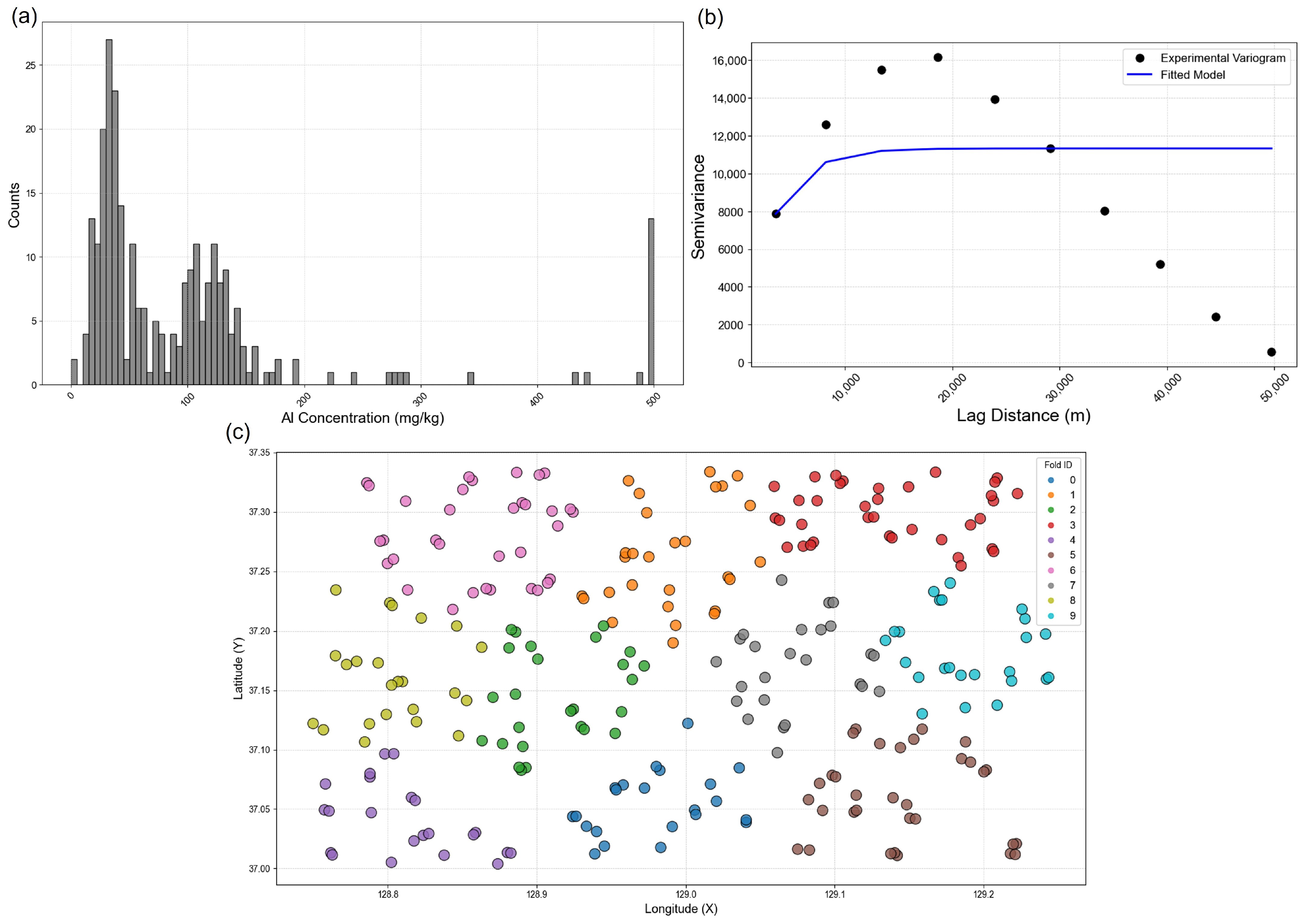
Table 4 summarizes the descriptive statistics of the target variable and auxiliary predictors in the original dataset. As shown in the histogram in Figure 4a, most Al observations were below 100 mg/kg, although several outliers reached approximately 500 mg/kg. These statistics indicate a strongly right-skewed distribution, with skewness of 2.53 and kurtosis of 6.23. This interpretation is also consistent with the median (62.50 mg/kg) relative to the mean (100.76 mg/kg).
To explore monotonic relationships between Al and the predictors, Spearman rank correlation coefficients are also reported in Table 4. Among the predictors, distance from fault showed the strongest negative association with Al (ρ = −0.46), while fault density showed the strongest positive association (ρ = 0.38). Before model training, continuous predictors were standardized within each spatial CV split using scaling parameters estimated from training folds and then applied to the corresponding held-out fold; the target variable (Al) remained in its original unit (mg/kg).
In addition, the empirical semivariogram of raw Al concentrations (Figure 4b) was examined as an exploratory analysis of spatial dependence, suggesting the presence of nonzero autocorrelation at short lag distances. Together, these distributional and spatial characteristics suggest that both nonlinear predictor effects and residual spatial dependence may be relevant, thereby motivating the subsequent comparison of standalone ML, standalone GS, and residual kriging hybrid models under spatial validation. The 10-fold spatial CV folds were generated by K-means clustering of the sample locations (Figure 4c) to reduce spatial information leakage between training and test subsets during model validation.

3.2. Prediction of Al Concentrations Distribution

3.2.1. Standalone ML and GS Results

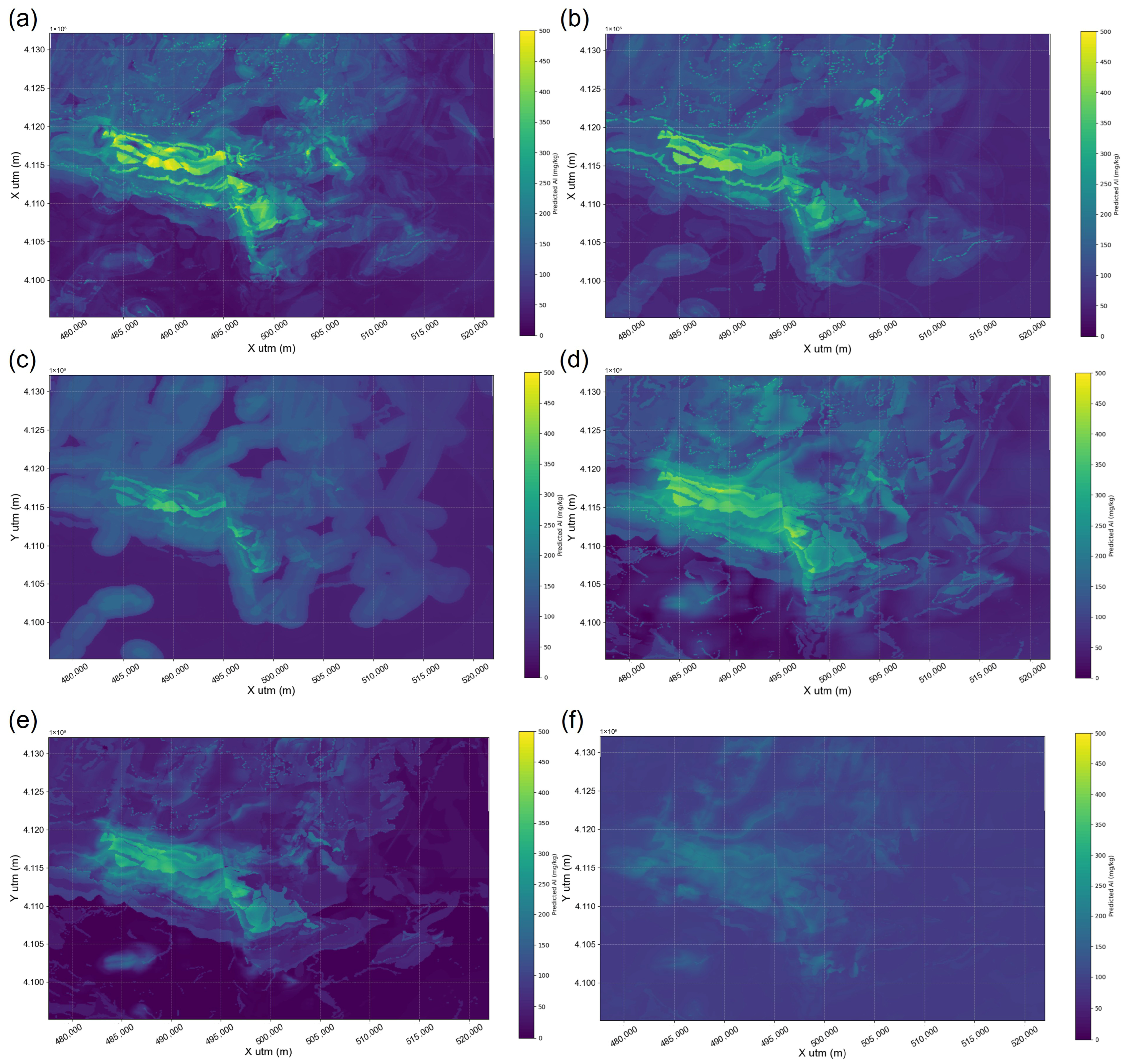
Figure 5 presents maps of predicted Al concentrations (mg/kg) generated by six ML models (RF, XGB, ADA, ResNet, U-Net, and STN) using the same predictor set: UTM coordinates, grouped lithologic classes, magnetic anomaly, gravity anomaly, fault density, distance from faults, and distance from deposits. Although all models used the same inputs, the predicted spatial patterns varied across model architectures. Under the 10-fold spatial CV, the tree-based ensembles achieved the best overall prediction performance based on aggregated OOF predictions, with RF performing best (RMSE = 93.66 mg/kg, relRMSE = 0.835, predictive R2 = 0.301), followed by XGB (RMSE = 95.78 mg/kg, relRMSE = 0.853, predictive R2 = 0.269) and ADA (RMSE = 107.14 mg/kg, relRMSE = 0.955, predictive R2 = 0.085). Fold-wise results are summarized in Table 5 and show substantial variability across spatial folds, with RMSE standard deviations of approximately 41~47 mg/kg across the ML models.
The NN-based models still showed lower prediction accuracy than the best tree-based ensembles for this dataset (n = 272) when assessed using aggregated OOF predictions, but their relative performance differed across architectures. ResNet yielded an OOF RMSE of 107.78 mg/kg, relRMSE of 1.070, and predictive R2 of 0.074, whereas U-Net achieved the best overall performance among the NN-based models (OOF RMSE = 103.70 mg/kg, relRMSE = 1.029, predictive R2 = 0.143), followed by STN (OOF RMSE = 106.95 mg/kg, relRMSE = 1.061, predictive R2 = 0.089). As a supplementary diagnostic, fold-wise predictive R2 values remained highly variable and negative on average across all NN-based models (Table 5), indicating that some held-out spatial folds were more difficult to predict than a mean-baseline within those folds. Visual inspection of Figure 5 suggests that RF (Figure 5a) and XGB (Figure 5b) preserved sharper local heterogeneity, whereas the NN-based models generated more spatially continuous regional patterns. In particular, the U-Net map (Figure 5e) delineates the main anomalous zone in the central-western part of the study area as a broader and more laterally connected high-prediction belt. Compared with ResNet and STN, U-Net therefore appears to represent the dominant regional pattern more clearly, although this regional continuity did not translate into performance superior to that of the best tree-based ensembles. STN (Figure 5f) reproduced some structural patterns, but this did not translate into a quantitative advantage over U-Net. These maps are shown in the original unit of mg/kg and should therefore be interpreted together with the quantitative metrics in Table 5 rather than as normalized values.
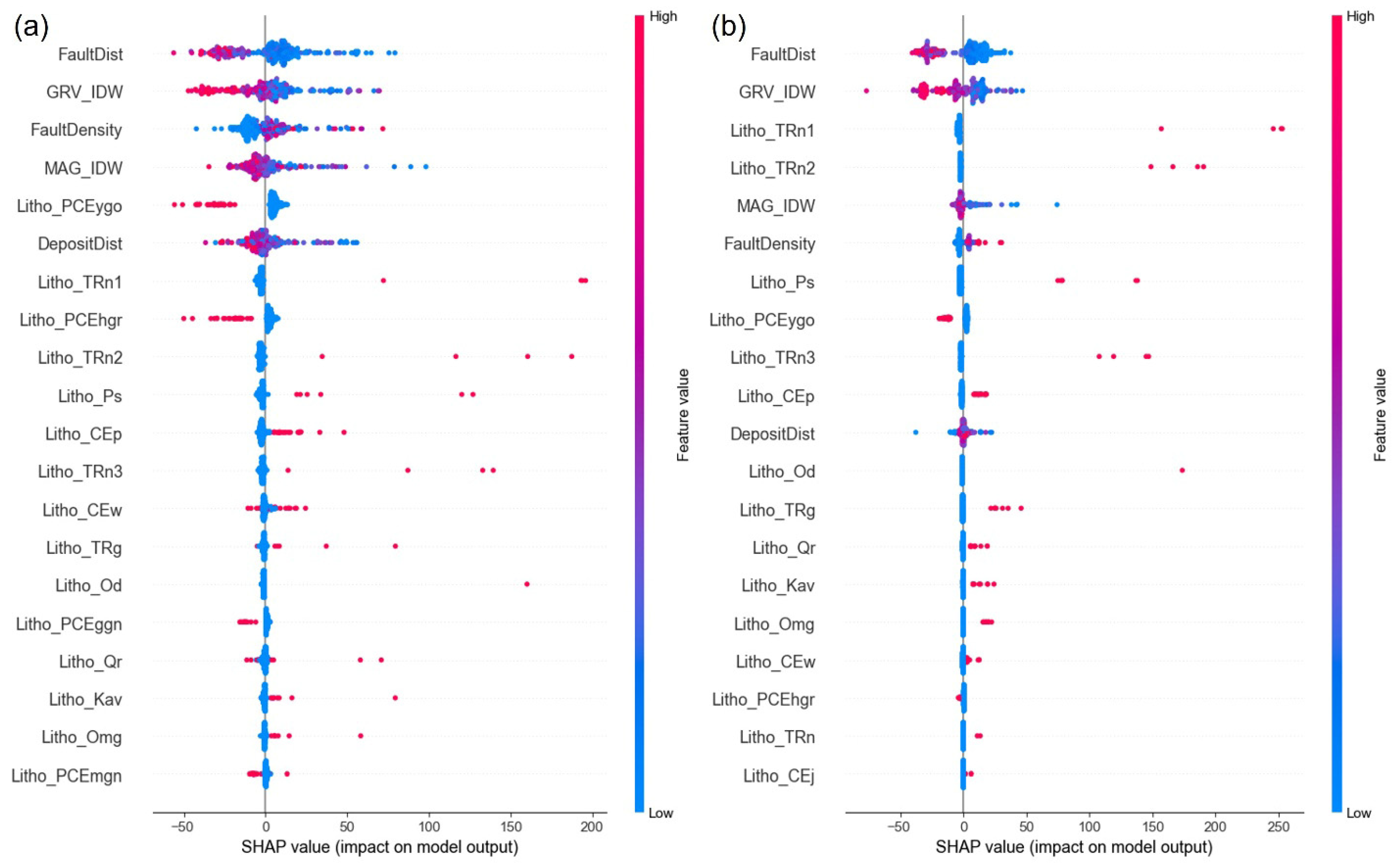
To reduce reliance on visual interpretation alone, predictor contributions were further examined using Shapley Additive Explanations (SHAP) for the two best-performing tree-based models, RF and XGB (Figure 6). In both models, the most influential predictors were distance from fault (FaultDist) and gravity anomaly (GRV_IDW), indicating that structural proximity and gravity anomaly were major controls on predicted Al concentrations. For FaultDist, shorter distances contributed positively to model output, whereas larger distances contributed negatively, implying higher predicted Al concentrations closer to faults. Beyond these common drivers, the two models differed in how they used auxiliary information. RF showed relatively stronger contributions from fault density and, secondarily, magnetic anomaly, with influence distributed across multiple lithologic classes. In contrast, XGB relied more strongly on a smaller subset of lithologic classes (notably Litho_TRn1 and Litho_TRn2), which produced large positive contributions for specific observations. Overall, the SHAP analysis suggests that both tree-based models capture a combination of structural and lithologic controls, although RF distributes importance more broadly whereas XGB concentrates it more strongly on a limited set of predictors.
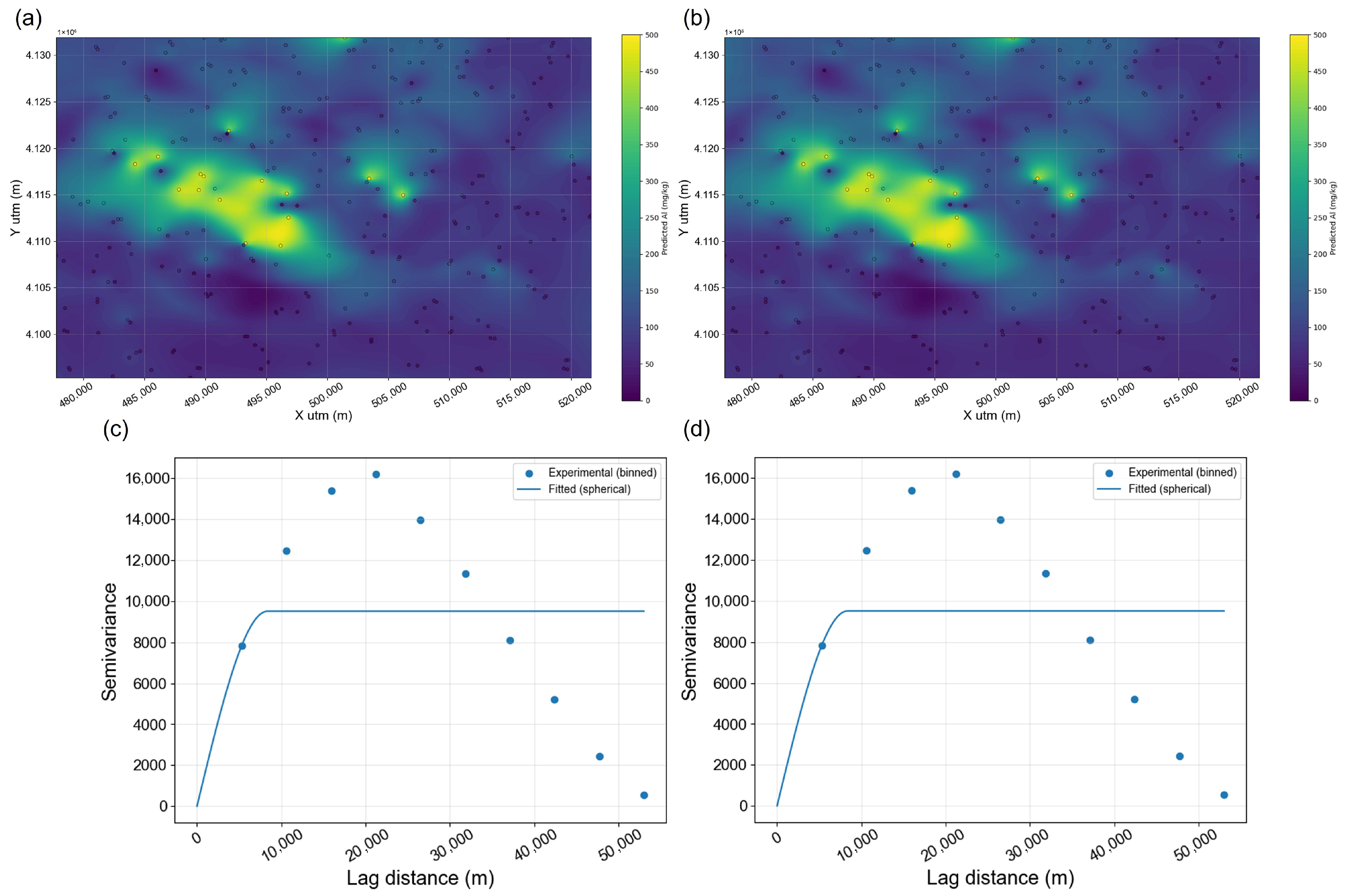
Using the same fold-wise variogram-fitting procedure described in Section 2.2.2, we evaluated OK and UK as GS baselines for Al interpolation (Figure 7). Figure 7 shows predicted Al concentrations in mg/kg, not normalized values. Under 10-fold Spatial CV, OK and UK showed comparable performance (fold-wise RMSE mean ± standard deviation: 93.95 ± 29.39 for OK and 96.28 ± 42.72 for UK), and their aggregated OOF metrics were also similar (OK: RMSE = 99.53, relRMSE = 0.887, R2 = 0.211; UK: RMSE = 107.48, relRMSE = 0.958, R2 = 0.079). Relative to the GS baselines, the best tree-based ML model (RF) showed slightly better aggregated OOF performance than OK, whereas UK performed similarly to the lower-performing ML models. As representative examples, Figure 7c,d show spherical variogram fits obtained within the spatial CV procedure; one representative fit yielded a range of approximately 8360 m, a sill of approximately 9521, and a nugget of 0. The corresponding maps (Figure 7a,b) show broadly similar spatial patterns, with only subtle differences in the central high-concentration zone. Overall, under the coordinate-based drift settings used here, UK did not provide consistent improvement over OK.

3.2.2. Residual Diagnostics and Hybrid Prediction Maps

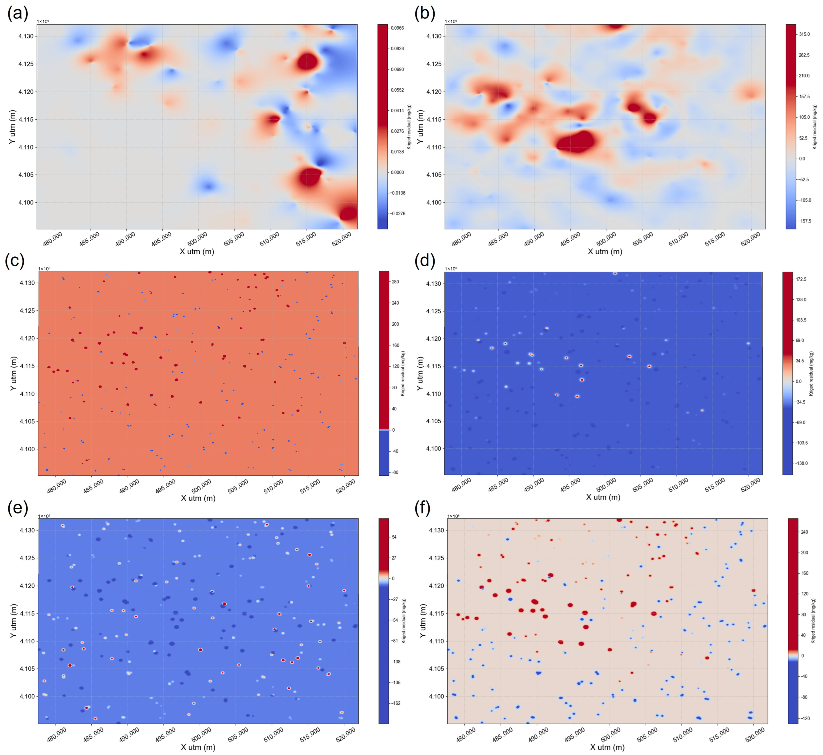
Visual comparison of predicted Al concentration maps alone is insufficient for evaluating prediction performance. Accordingly, we examined cross-fitted prediction residuals (observed minus OOF-predicted values at sampling locations) for each ML backbone and interpolated these residuals using OK to visualize the spatial structure of systematic error (Figure 8). Residual values are also shown in the original unit of mg/kg, not as normalized values. Positive residuals indicate underprediction, whereas negative residuals indicate overprediction. The color scale was centered symmetrically at zero, and the displayed range was defined using the central 99% of absolute residual values to reduce the visual influence of extreme outliers.
Across the models, the OK-based residual surfaces revealed zones of systematic under- and overprediction. For RF, XGB, and STN, residual fields retained relatively localized patches around the central high-concentration zone (Figure 8a,b,f), suggesting that some spatially structured residual error remained after the ML trend prediction. In contrast, ADA, ResNet, and U-Net showed more spatially diffuse residual patterns with less clearly localized structure (Figure 8c–e).
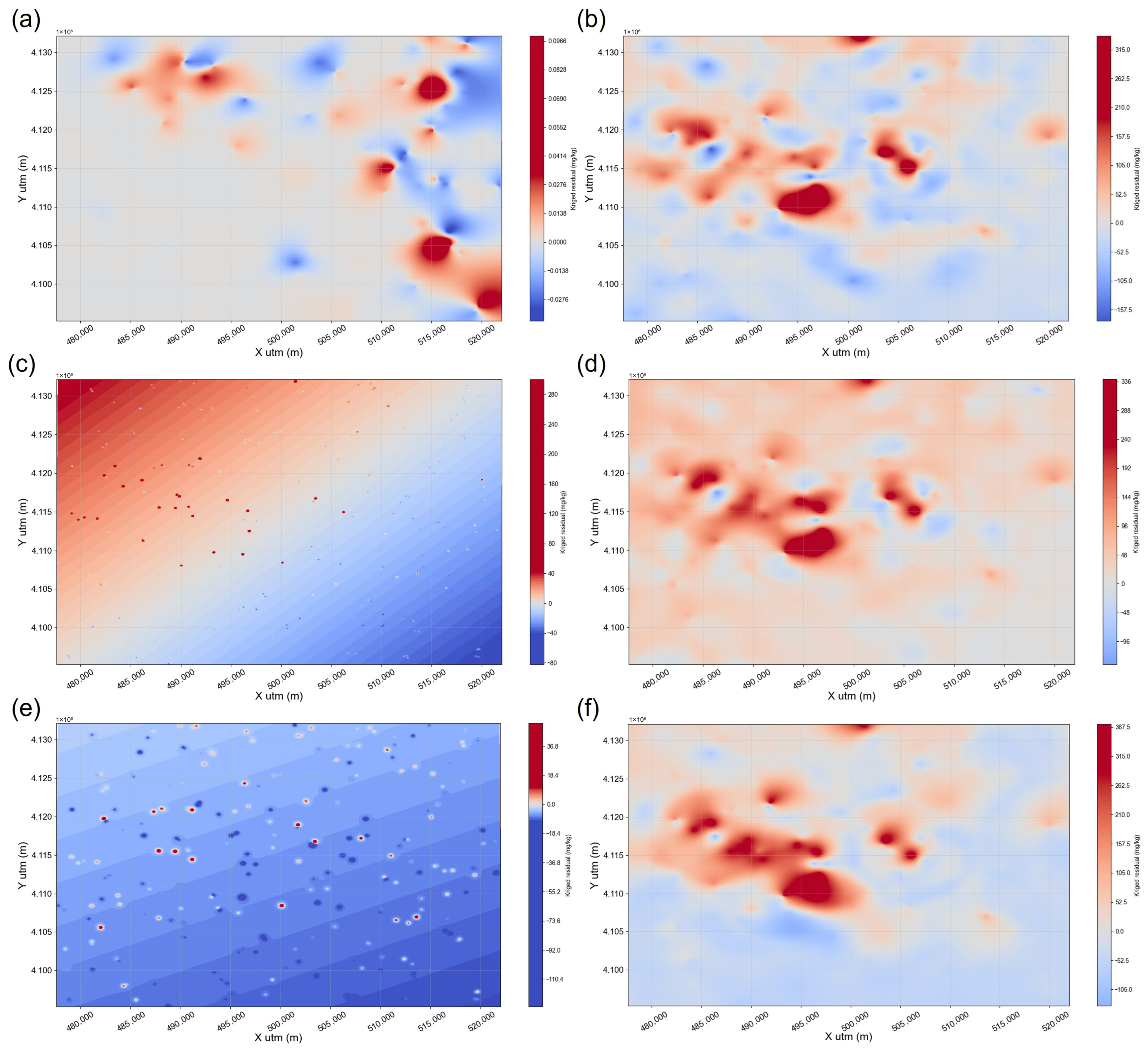
Figure 9 shows residual surfaces obtained using UK for the same six ML backbones. Relative to the OK-based residual maps in Figure 8, some UK-based residual surfaces display stronger large-scale gradients, reflecting the effect of the coordinate-based drift term used in UK. This tendency is most apparent for ADA, ResNet, and U-Net (Figure 9c–e), whereas RF, XGB, and STN (Figure 9a,b,f) preserve localized structure around the central anomalous zone.
Importantly, the residual-interpolation maps are presented for qualitative diagnosis only and were not used as a performance criterion. Prediction performance was assessed exclusively through the spatial CV framework, in which model fitting, hyperparameter tuning, variogram fitting, and residual kriging were all conditioned on the training folds, while the held-out fold was reserved exclusively for performance evaluation. Under this design, aggregated OOF RMSE values for the hybrid models remained substantial (93.662–106.779 mg/kg; Table 6), confirming that performance was evaluated out of sample rather than reconstructed from in-sample residual fitting.
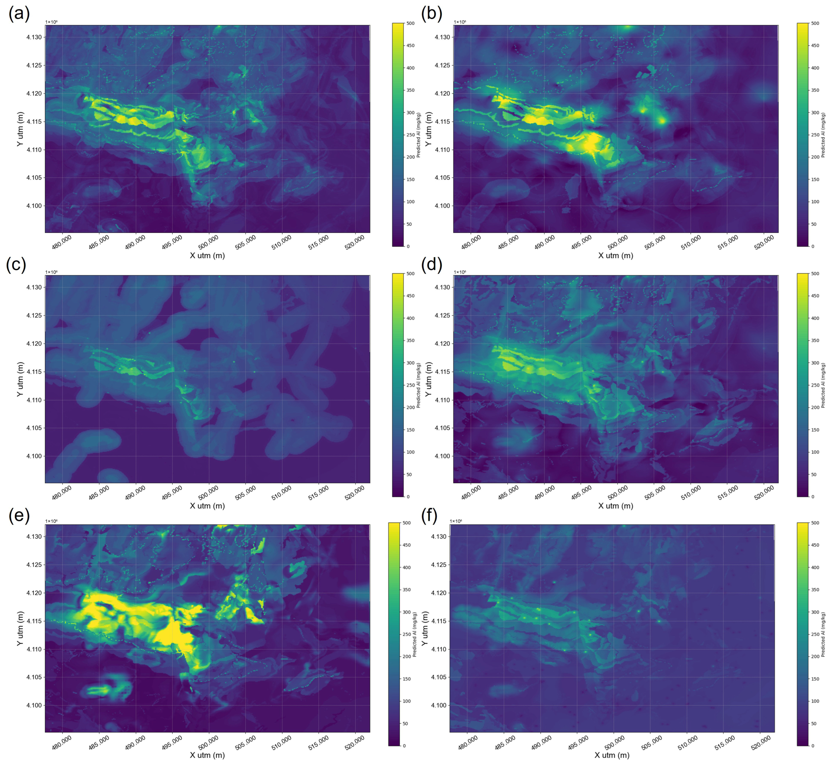
Final hybrid Al concentration maps were generated under the RK framework by adding the kriged residual surface to the ML trend prediction. Figure 10 presents the OK-integrated hybrid maps in the original unit of mg/kg. Relative to the corresponding ML-only maps, the OK-based hybrids introduced spatially coherent corrections in areas of systematic under- or overprediction while largely preserving the broader spatial patterns learned by each ML backbone. The tree-based hybrids (RF–OK, XGB–OK, and ADA–OK; Figure 10a–c) retained comparatively finer local structure in the central anomalous region, whereas the NN-based hybrids (ResNet–OK, U-Net–OK, and STN–OK; Figure 10d–f) preserved smoother transitions inherited from their ML trend components.
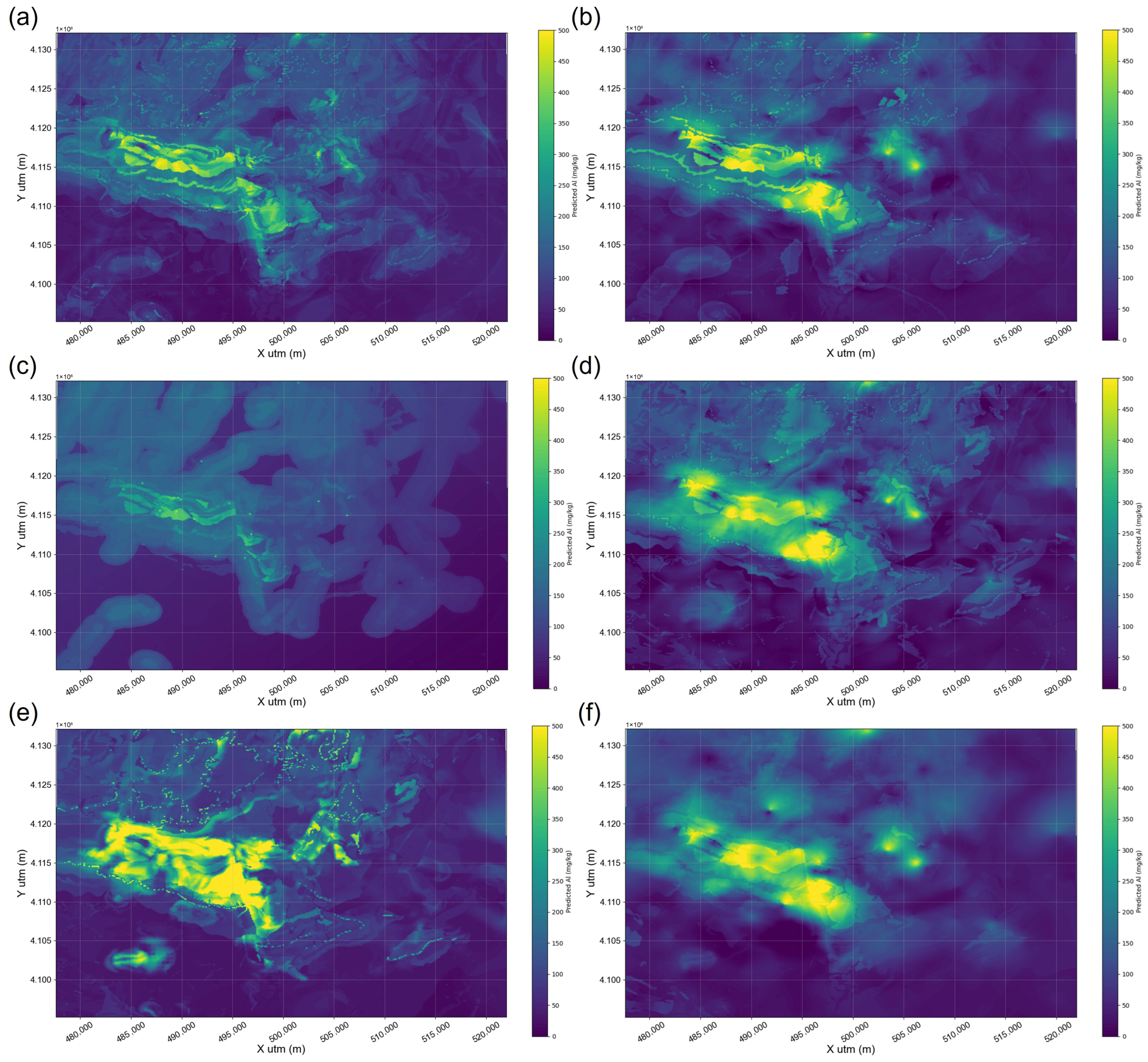
Figure 11 shows the corresponding UK-integrated hybrid maps, also reported in mg/kg. Relative to OK-integrated hybrids (Figure 10), UK-based hybrids exhibit similar large-scale Al distributions, but the residual correction can additionally reflect the coordinate-based drift component used in UK. For some backbones (e.g., ADA, ResNet, and U-Net), this leads to more regionally smoothed correction patterns consistent with the broader gradients observed in Figure 9, whereas for RF, XGB, and STN residual corrections remain more localized. As in the GS-only comparison, visual inspection alone was not used to infer predictive superiority; instead, the hybrid variants were compared using spatial CV and aggregated OOF metrics (Table 6).
Table 6 summarizes the prediction performance of the integrated ML–GS models under the RK framework. Based on aggregated OOF RMSE, the effect of residual kriging was model dependent rather than uniformly beneficial. For RF, OK- and UK-based integration yielded essentially identical results and did not materially improve upon the standalone RF model (RF–OK/RF–UK: RMSE = 93.662–93.663 mg/kg, predictive R2 = 0.301). For XGB and ADA, UK-based integration produced modest improvements relative to OK (XGB–UK: RMSE = 93.922 mg/kg, predictive R2 = 0.297; XGB–OK: RMSE = 95.009 mg/kg, predictive R2 = 0.281). For ResNet, OK-based integration outperformed UK-based integration (ResNet–OK: RMSE = 96.709 mg/kg, predictive R2 = 0.255; ResNet–UK: RMSE = 100.171 mg/kg, predictive R2 = 0.200). For U-Net, UK-based integration showed a modest advantage over OK-based integration (U-Net–UK: RMSE = 99.178 mg/kg, predictive R2 = 0.216; U-Net–OK: RMSE = 100.107 mg/kg, predictive R2 = 0.201). For STN, OK-based integration improved performance relative to both the standalone STN model and STN–UK, whereas UK-based integration performed worst among the STN hybrids (STN–OK: RMSE = 99.820 mg/kg, predictive R2 = 0.206; STN–UK: RMSE = 106.779 mg/kg, predictive R2 = 0.092). Overall, the best aggregated OOF performance remained RF-based, and hybrid gains were modest and backbone dependent rather than universal.
For STN, the discrepancy between fold-wise mean RMSE and aggregated OOF RMSE indicates that these two summaries emphasize different aspects of predictive behavior across spatial folds. For this reason, both summaries are reported, although aggregated OOF RMSE was treated as the primary basis for comparison.

3.2.3. Comparative Prediction Performance of Standalone and Integrated Models

Table 7 summarizes the aggregated OOF prediction performance of the standalone models under the 10-fold spatial CV framework. Among the ML models, tree-based ensembles achieved the strongest performance, with RF performing best (RMSE = 93.66 mg/kg, relRMSE = 0.835, predictive R2 = 0.301), followed by XGB (RMSE = 95.78 mg/kg, relRMSE = 0.853, predictive R2 = 0.269). In contrast, the NN-based models showed higher OOF RMSE (106.64–109.25 mg/kg) and lower predictive R2 values (0.049–0.094). The GS baselines showed intermediate performance (OK: RMSE = 99.53 mg/kg, predictive R2 = 0.211; UK: RMSE = 107.48 mg/kg, predictive R2 = 0.079). Overall, for this dataset, the best-performing ML models provided lower prediction error than the kriging-only baselines.
Table 8 compares the aggregated OOF performance of RK-based integrated ML–GS models across ML backbones and kriging variants. Relative to the corresponding standalone ML models in Table 7, residual kriging integration improved prediction accuracy for several backbones, but the magnitude and direction of the effect were clearly backbone dependent rather than uniform. For example, ADA improved from an RMSE of 107.14 mg/kg (predictive R2 = 0.085) to 99.360–98.545 mg/kg (predictive R2 = 0.213–0.226), and ResNet improved from 109.25 mg/kg (predictive R2 = 0.049) to 96.709–100.171 mg/kg (predictive R2 = 0.200–0.255). In contrast, RF showed essentially no change after integration (RMSE 93.662–93.663 mg/kg; predictive R2 = 0.301), while STN exhibited a strong sensitivity to the kriging variant (STN–OK: RMSE = 99.820 mg/kg, predictive R2 = 0.206; STN–UK: RMSE = 106.779 mg/kg, predictive R2 = 0.092). Overall, neither OK nor UK showed a consistent advantage across all backbones: UK improved OOF performance for XGB, ADA, and U-Net, whereas OK performed better for ResNet and STN, and RF showed no practical difference between the two variants.
To formally examine whether observed fold-wise differences were statistically supported, we conducted paired tests across the 10 spatial folds for (i) OK versus UK within each backbone (difference = UK − OK) and (ii) standalone ML versus hybrid performance within each backbone (difference = Hybrid − ML). We report both paired t-tests and Wilcoxon signed-rank tests, with Holm-adjusted p-values to account for multiple comparisons (Appendix A, Table A1, Table A2, Table A3 and Table A4). After Holm correction, no statistically significant differences were detected between OK and UK for any backbone on either RMSE or predictive R2 (Table A1 and Table A2). For standalone ML versus hybrid comparisons, most backbones did not show statistically significant differences after multiple-comparison correction. The only significant result was a reduction in RMSE for U-Net–UK relative to standalone U-Net (mean fold-wise RMSE difference = −12.757 mg/kg; Holm-adjusted paired t-test p = 0.0186; Holm-adjusted Wilcoxon p = 0.0469), whereas differences in predictive R2 were not significant (Table A3 and Table A4). Taken together, the effect of hybridization was heterogeneous across backbones and should be interpreted in conjunction with effect sizes, fold-wise variability, and limited statistical power, rather than as evidence of universal superiority.

4. Discussion

4.1. Bias-Aware Evaluation of Hybrid ML–GS Prediction Under Spatial Cross-Validation

Recent studies have demonstrated the practical utility of ML–GS hybrid prediction for spatial mapping; however, many applications evaluate only a limited range of model combinations and may rely on residual constructions that are optimistically biased when residuals are derived in-sample. Building on established practices in spatially explicit model assessment and RK-type workflows, this study provides a consistent comparison across six ML backbones (three tree-based and three NN-based models) and two kriging variants (OK and UK) under a 10-fold spatial CV design. Within each outer CV split, residual modeling—including variogram fitting and residual kriging—was conditioned strictly on training data. When residuals were used for variogram characterization, they were obtained from the training fold by within-training CV (i.e., cross-fitted residuals) to reduce optimistic bias while preventing leakage from the held-out fold.
Across the evaluated backbones, OK and UK did not show a consistent performance separation, suggesting that the coordinate-based drift specification used here was not uniformly beneficial for this dataset. Likewise, residual kriging did not provide a universal gain over standalone ML predictions; instead, the effect of hybridization was clearly backbone dependent. In practical terms, these results suggest that ML–GS integration should be viewed as a conditional error-correction mechanism rather than as a uniformly superior strategy. For some ML backbones, residual kriging improved predictions by capturing remaining spatial dependence in the model errors, whereas for already strong models the marginal benefit was negligible. Accordingly, the main implication of this study is not that hybridization is always superior, but that a spatially explicit, bias-aware evaluation helps identify when and for which model architectures residual spatial modeling yielded reproducible gains.

4.2. Uncertainty Quantification, Statistical Testing, and Data Limitations

Rather than relying on a single train/test split, prediction performance was evaluated using a 10-fold spatial CV scheme that generates repeated out-of-sample predictions and reduces dependence on any particular partition. Uncertainty in performance estimates was summarized using fold-to-fold variability and 95% confidence intervals for RMSE and predictive R2, which is important given the heterogeneous difficulty of predicting held-out spatial clusters. In addition, fold-wise paired tests were conducted to examine whether differences between model variants (OK vs. UK, and standalone ML vs. hybrid within the same backbone) were statistically supported. Holm-adjusted p-values were used to account for multiple comparisons, and full results are reported in Appendix A. Consistent with the CV summary metrics, these tests indicate that most observed differences were not statistically significant after correction, reinforcing the need to interpret results in terms of effect size and uncertainty rather than as evidence of uniform superiority.
Several limitations should be considered when interpreting these findings. First, observations are spatially and lithologically imbalanced, which can increase uncertainty in sparsely sampled zones and lead to spatially heterogeneous generalization. Second, the relatively small sample size (n = 272) and the gridding setup can limit the effective training signal available to higher-capacity models and amplify fold-to-fold variability under the spatial CV. Future work should prioritize more balanced or targeted sampling and incorporate higher-resolution covariates (e.g., litho-geochemical proxies, remote-sensing-derived indices, or structural complexity measures) to better capture local variability and improve spatial transferability. From a methodological perspective, broader benchmark comparisons—including simpler parametric baselines, additional GS baselines, and alternative drift specifications—would further clarify when hybridization provides benefits beyond established interpolation approaches.

5. Conclusions

We conducted a systematic evaluation of twelve ML–GS hybrid configurations by combining the six ML models (tree-based ensembles and NN-based models) with the two kriging methods (OK and UK) to predict the spatial distribution of Al concentrations in the study area. Model performance was assessed under a 10-fold spatial CV framework, and the residual kriging component—including variogram fitting—was conditioned strictly on training data within each split. Cross-fitted residuals were used for residual variogram characterization to reduce optimistic bias and prevent data leakage.
Across the evaluated backbones, OK and UK did not exhibit a consistent performance separation under the coordinate-based drift specification used here. More importantly, residual kriging integration did not provide a universal gain over standalone ML predictions. Instead, the effect of hybridization was backbone dependent. For already strong ML backbones, the marginal benefit of residual correction was negligible; for weaker backbones, residual kriging provided measurable improvements by correcting spatially structured errors that remained after ML trend prediction. Among the evaluated models, RF-based predictions showed the strongest overall out-of-sample performance, while hybrid improvements for other backbones were generally modest.
Overall, these results indicate that ML–GS integration should be viewed as a bias-aware strategy for identifying when residual spatial modeling adds value, rather than as a guarantee of improved accuracy. Because the analysis was conducted on a single case-study dataset with a relatively small sample size (n = 272), the findings should be interpreted as case specific rather than as fully general conclusions. Nevertheless, the broader contribution of this study lies in providing a transferable evaluation framework for comparing standalone ML, GS and RK-based hybrids models under spatially explicit validation while minimizing optimistic bias and data leakage. For practitioners and researchers working on other spatial prediction problems, this framework can serve as a practical reference for testing whether hybridization is warranted for a given dataset, identifying when residual spatial correction provides meaningful benefit, and avoiding the assumption that additional model complexity will necessarily improve prediction performance. Future work should evaluate larger and more balanced datasets, incorporate richer covariates, and compare hybrid models against broader benchmark sets, including simpler parametric and additional geostatistical baselines, to examine the transferability of these findings across other case studies and application domines.

Author Contributions

Hosang Han: methodology, conceptualization, analysis, validation, visualization, and writing the original draft; Jangwon Suh: conceptualization, supervision, project administration, writing the review, and editing. All authors have read and agreed to the published version of the manuscript.

Funding

This work was supported by (1) the Energy & Mineral Resources Development Association of Korea (EMRD) grant funded by the Korean government (MOTIE) (2021060001, Data science-based oil/gas exploration consortium) and (2) the Korea Institute of Energy Technology Evaluation and Planning (KETEP) and the Ministry of Climate, Energy & Environment (MCEE) of the Republic of Korea (No. RS-2025-02310648).

Data Availability Statement

The original contributions presented in this study are included in the article. Further inquiries can be directed to the corresponding author.

Conflicts of Interest

Author Hosang Han was employed by the company Exploration & Mining Research Team, Korea Mine Rehabilitation and Mineral Resources Corporation. The remaining authors declare that the research was conducted in the absence of any commercial or financial relationships that could be construed as a potential conflict of interest.

Abbreviations

The following abbreviations are used in this manuscript:
MLMachine Learning
AlAluminum
RFRandom Forest
XGBXGBoost
ADAAdaBoost
STNSpatial Transformer
OKOrdinary Kriging
UKUniversal Kriging
CVCross-validation
OOFOut-Of-Fold
GSGeostatistics
FSEFeature Space Enhancement
RKRegression Kriging
NNNeural Network
EDAExploratory Data Analysis
TiO2Titanium Dioxide
UTMUniversal Transverse Mercator
MSEMean Squared Error
RMSERoot Mean Squared Error
relRMSERelative Root Mean Squared Error
Predictive R2Predictive Coefficient of Determination
SSESum of Squared Residuals
SSTTotal Sum of Squares

Appendix A. Fold-Wise Paired Statistical Comparisons

Appendix A.1. OK Versus UK Within Each Backbone (Difference = UK − OK, n = 10 Spatial Folds)

Table A1. Fold-wise paired tests for RMSE: OK versus UK within each backbone.
BackboneMean Diff (UK − OK)tpHolm p95% CI
RF−0.000−0.0001.0001.000[−0.003, 0.003]
XGB−2.056−0.8530.4161.000[−7.508, 3.396]
ADA−2.114−0.6430.5361.000[−9.550, 5.322]
ResNet+6.363+1.8940.0910.544[−1.235, 13.961]
UNet−2.556−1.0460.3231.000[−8.084, 2.972]
STN−2.902−0.3670.7221.000[−20.783, 14.979]
Table A2. Fold-wise paired tests for predictive R2: OK versus UK within each backbone.
BackboneMean Diff (UK − OK)tpHolm p95% CI
RF−0.00010−0.5570.5911.000[−0.00051, 0.00031]
XGB+0.3040+1.2660.2371.000[−0.239, 0.847]
ADA−0.1734−0.2940.7751.000[−1.506, 1.159]
ResNet−0.7445−1.4660.1771.000[−1.894, 0.405]
UNet+0.5321+1.1440.2821.000[−0.520, 1.585]
STN+0.4670+0.6420.5371.000[−1.178, 2.112]

Appendix A.2. Standalone ML Versus Hybrid Models Within Each Backbone (Difference = Hybrid − ML, n = 10 Spatial Folds)

Table A3. Fold-wise paired tests for RMSE: standalone ML versus hybrid models within each backbone.
ComparisonMean Diff
(Hybrid − ML)
tpHolm pWilcoxon pHolm (Wilcoxon)
RF vs. RF–OK−0.003−0.2820.7851.0000.7501.000
RF vs. RF–UK−0.003−0.3000.7711.0000.6251.000
XGB vs. XGB–OK+0.546+0.4610.6561.0000.3751.000
XGB vs. XGB–UK−1.510−0.5530.5941.0000.5571.000
ADA vs. ADA–OK−4.283−1.2800.2321.0000.5571.000
ADA vs. ADA–UK−6.397−1.4040.1941.0000.2321.000
ResNet vs. ResNet–OK+3.692+1.0610.3171.0000.3221.000
ResNet vs. ResNet–UK+10.055+1.6270.1381.0000.4921.000
UNet vs. UNet–OK−10.201−3.0630.01350.14860.01950.2148
UNet vs. UNet–UK−12.757−4.4710.001550.01860.003910.0469
STN vs. STN–OK−1.483−0.3520.7331.0000.6951.000
STN vs. STN–UK−4.385−0.4420.6691.0000.4321.000
Table A4. Fold-wise paired tests for predictive R2: standalone ML versus hybrid models within each backbone.
ComparisonMean Diff (Hybrid − ML)tpHolm pWilcoxon pHolm (Wilcoxon)
RF vs. RF–OK+0.0003+0.8960.3941.0000.7501.000
RF vs. RF–UK+0.0002+0.8020.4431.0000.7501.000
XGB vs. XGB–OK−0.2189−1.3610.2071.0000.2111.000
XGB vs. XGB–UK+0.0851+0.4450.6671.0000.8461.000
ADA vs. ADA–OK−0.0078−0.1170.9101.0000.9221.000
ADA vs. ADA–UK−0.1812−0.3170.7581.0000.4321.000
ResNet vs. ResNet–OK−0.6500−1.3500.2101.0000.4321.000
ResNet vs. ResNet–UK−1.3945−1.4420.1831.0000.6251.000
UNet vs. UNet–OK+0.3868+0.5310.6081.0000.1051.000
UNet vs. UNet–UK+0.9189+1.9010.08981.0000.03710.445
STN vs. STN–OK−0.3622−1.7250.1191.0000.1931.000
STN vs. STN–UK+0.1048+0.1560.8791.0000.3221.000

References

  1. Gu, A. Geostatistical approaches for resource estimation in mining and exploration. J. Environ. Risk Assess. Remediat. 2023, 7, 182. [Google Scholar]
  2. Hack, D.R. Issues and Challenges in the Application of Geostatistics and Spatial-Data Analysis to the Characterization of Sand-And-Gravel Resources; U.S. Geological Survey: Reston, VA, USA, 2005. [Google Scholar]
  3. Cellmer, R. The possibilities and limitations of geostatistical methods in real estate market analyses. Real Estate Manag. Valuat. 2014, 22, 54–62. [Google Scholar] [CrossRef]
  4. Silva, V.M. On the classification and treatment of outliers in a spatial context: A Bayesian updating approach. REM-Int. Eng. J. 2021, 74, 379–389. [Google Scholar] [CrossRef]
  5. Battalgazy, N.; Valenta, R.; Gow, P.; Spier, C.; Forbes, G. Addressing geological challenges in mineral resource estimation: A comparative study of deep learning and traditional techniques. Minerals 2023, 13, 982. [Google Scholar] [CrossRef]
  6. Sowińska-Botor, J.; Mastej, W.; Maćkowski, T. Ranking of the utility of selected geostatistical interpolation methods in conditions of highly skewed seismic data distributions: A case study of the Baltic Basin (Poland). Gospod. Surowc. Min.-Miner. Resour. Manag. 2023, 39, 149–172. [Google Scholar] [CrossRef]
  7. Heaton, M.J.; Millane, A.; Rhodes, J.S. Adjusting for spatial correlation in machine and deep learning. arXiv 2024, arXiv:2410.04312. [Google Scholar] [CrossRef]
  8. Frank, J.K.; Suesse, T.; Brenning, A. An assessment of spatial random forests for environmental mapping: The case of groundwater nitrate concentration. Environ. Model. Softw. 2025, 193, 106626. [Google Scholar] [CrossRef]
  9. Patelli, L.; Cameletti, M.; Golini, N.; Ignaccolo, R. A Path in Regression Random Forest Looking for Spatial Dependence: A Taxonomy and a Systematic Review. In Advanced Statistical Methods in Process Monitoring, Finance, and Environmental Science; Knoth, S., Okhrin, Y., Otto, P., Eds.; Springer: Cham, Switzerland, 2024. [Google Scholar] [CrossRef]
  10. Chen, L.; Ren, C.; Li, L.; Wang, Y.; Zhang, B.; Wang, Z.; Li, L. A comparative assessment of geostatistical, machine learning, and hybrid approaches for mapping topsoil organic carbon content. ISPRS Int. J. Geo-Inf. 2019, 8, 174. [Google Scholar] [CrossRef]
  11. Song, Y.Q.; Yang, L.A.; Li, B.; Hu, Y.M.; Wang, A.L.; Zhou, W.; Cui, X.S.; Liu, Y.L. Spatial prediction of soil organic matter using a hybrid geostatistical model of an extreme learning machine and ordinary kriging. Sustainability 2017, 9, 754. [Google Scholar] [CrossRef]
  12. Mohammadpour, M.; Roshan, H.; Arashpour, M.; Masoumi, H. Machine learning assisted kriging to capture spatial variability in petrophysical property modelling. Mar. Pet. Geol. 2024, 167, 106967. [Google Scholar] [CrossRef]
  13. Su, H.; Shen, W.; Wang, J.; Ali, A.; Li, M. Machine learning and geostatistical approaches for estimating aboveground biomass in Chinese subtropical forests. For. Ecosyst. 2020, 7, 64. [Google Scholar] [CrossRef]
  14. Adeniyi, O.D.; Brenning, A.; Maerker, M. Spatial prediction of soil organic carbon: Combining machine learning with residual kriging in an agricultural lowland area (Lombardy region, Italy). Geoderma 2024, 448, 116953. [Google Scholar] [CrossRef]
  15. Han, H.; Suh, J. Spatial prediction of soil contaminants using a hybrid random forest–ordinary kriging model. Appl. Sci. 2024, 14, 1666. [Google Scholar] [CrossRef]
  16. Sun, W.; Cao, S.; Cai, C.; Kong, F.; Liu, J. Biomass distribution characteristics of Picea schrenkiana var. tianschanica by integrating ordinary kriging and machine learning. In Proceedings of the 2024 Asia-Pacific Conference on Software Engineering, Social Network Analysis and Intelligent Computing (SSAIC); IEEE: New York, NY, USA, 2024; pp. 691–694. [Google Scholar] [CrossRef]
  17. Wu, Z.; Yao, F.; Zhang, J.; Liu, H. Estimating forest aboveground biomass using a combination of geographical random forest and empirical Bayesian kriging models. Remote Sens. 2024, 16, 1859. [Google Scholar] [CrossRef]
  18. Murphy, B.; Yurchak, R.; Müller, S. GeoStat-Framework/PyKrige: V1.7.2, v1.7.2; Zenodo: Geneva, Switzerland, 2024. [CrossRef]
  19. Korea Institute of Geoscience and Mineral Resources. Exploration and Utilization Technology Development for Rare Metal Resources in Korea: Excerpt from the Myeonsan Formation in the Taebaek Area (Research Report). 2022. Available online: https://www.kigam.re.kr/board.es?mid=a10704000000&bid=0028&list_no=51290&act=view (accessed on 11 April 2026).
  20. Kim, Y.; Moscoso-Pinto, F.; Seo, J.; Cho, K.; Cho, J.; Lee, S.; Kim, H. Mineral processing characteristics of titanium ore mineral from Myeosan Layer in domestic Taebaek area. Resour. Recycl. 2023, 32, 54–66. [Google Scholar] [CrossRef]
  21. Park, Y.; Rim, H.; Lim, M.; Shin, Y. The magnetic anomaly map of Korea. Geophys. Geophys. Explor. 2019, 22, 29–36. [Google Scholar] [CrossRef]
  22. Shin, Y.; Ko, I. Gravity anomaly in the Taebaeksan mineralized zone. J. Geol. Soc. Korea 2019, 55, 403–413. [Google Scholar] [CrossRef]
  23. Korea Institute of Geoscience and Mineral Resources. Geo Big Data Open Platform. Available online: https://data.kigam.re.kr/ (accessed on 16 March 2025).
  24. Breiman, L. Random forests. Mach. Learn. 2001, 45, 5–32. [Google Scholar] [CrossRef]
  25. Chen, T.; Guestrin, C. XGBoost: A scalable tree boosting system. In Proceedings of the 22nd ACM SIGKDD International Conference on Knowledge Discovery and Data Mining; ACM: New York, NY, USA, 2016; pp. 785–794. [Google Scholar]
  26. Freund, Y.; Schapire, R.E. A decision-theoretic generalization of on-line learning and an application to boosting. J. Comput. Syst. Sci. 1997, 55, 119–139. [Google Scholar] [CrossRef]
  27. He, K.; Zhang, X.; Ren, S.; Sun, J. Deep residual learning for image recognition. In Proceedings of the IEEE Conference on Computer Vision and Pattern Recognition; IEEE: New York, NY, USA, 2016; pp. 770–778. [Google Scholar]
  28. Ronneberger, O.; Fischer, P.; Brox, T. U-net: Convolutional networks for biomedical image segmentation. In Medical Image Computing and Computer-Assisted Intervention–MICCAI 2015: 18th International Conference, Munich, Germany, 5–9 October 2015; Proceedings, Part III; Springer: Cham, Switzerland, 2015; pp. 234–241. [Google Scholar] [CrossRef]
  29. Jaderberg, M.; Simonyan, K.; Zisserman, A. Spatial transformer networks. Adv. Neural Inf. Process. Syst. 2015, 28. [Google Scholar]
  30. Cressie, N. The origins of kriging. Math. Geol. 1990, 22, 239–252. [Google Scholar] [CrossRef]
  31. Journel, A.G.; Huijbregts, C.J. Mining Geostatistics; Academic Press: London, UK, 1976. [Google Scholar]
  32. Goovaerts, P. Geostatistics for Natural Resources Evaluation; Oxford University Press: New York, NY, USA, 1997. [Google Scholar]
  33. Hyndman, R.J.; Koehler, A.B. Another look at measures of forecast accuracy. Int. J. Forecast. 2006, 22, 679–688. [Google Scholar] [CrossRef]
Figure 1. Workflow of research methodology.
Ijgi 15 00175 g001
Figure 2. Distribution of Al concentration data (mg/kg) from surface survey samples in the study area.
Ijgi 15 00175 g002
Figure 3. Auxiliary variables used for spatial prediction. (a) Grouped lithologic classes, (b) magnetic anomaly, (c) gravity anomaly, (d) fault density, (e) distance from faults, and (f) distance from deposits.
Ijgi 15 00175 g003
Figure 4. Exploratory data analysis of the original dataset. (a) Histogram of Al concentrations (mg/kg), (b) exploratory empirical semivariogram of raw Al concentrations, and (c) spatial CV folds generated by K-means clustering.
Ijgi 15 00175 g004
Figure 5. Maps of Al concentrations predicted by ML models (mg/kg). (a) RF, (b) XGB, (c) ADA, (d) ResNet, (e) U-Net, and (f) STN.
Ijgi 15 00175 g005
Figure 6. SHAP summary plots for the two best-performing tree-based models: (a) RF and (b) XGB.
Ijgi 15 00175 g006
Figure 7. GS baselines maps of Al concentrations interpolated using kriging variants (mg/kg). (a) OK, (b) UK, (c) Representative fitted semivariogram from a training fold (OK), and (d) Representative fitted semivariogram from a training fold (UK).
Ijgi 15 00175 g007
Figure 8. Residual maps of ML-based interpolated by OK (mg/kg). (a) RF, (b) XGB, (c) ADA, (d) ResNet, (e) U-Net, and (f) STN.
Ijgi 15 00175 g008
Figure 9. Residual maps of ML-based residuals interpolated by UK (mg/kg). (a) RF, (b) XGB, (c) ADA, (d) ResNet, (e) U-Net, and (f) STN.
Ijgi 15 00175 g009
Figure 10. Al concentration maps predicted using integrated ML–OK interpolation models (mg/kg). (a) RF–OK, (b) XGB–OK, (c) ADA–OK, (d) ResNet–OK, (e) U-Net–OK, and (f) STN–OK.
Ijgi 15 00175 g010
Figure 11. Al concentration maps predicted using integrated ML–UK interpolation models (mg/kg). (a) RF–UK, (b) XGB–UK, (c) ADA–UK, (d) ResNet–UK, (e) U-Net–UK, and (f) STN–UK.
Ijgi 15 00175 g011
Table 1. Recent studies on hybrid ML–GS interpolation models.
ReferencesML ModelGS MethodHybrid StrategyTarget
[10]Support vector regression,
Artificial neural network
Ordinary kriging,
Geographically weighted regression
RKSoil organic carbon
[11]Extreme learning machineOrdinary krigingRKSoil organic matter
[12]Least squared support vector regressionSimple krigingRKPetrophysical property modeling
[13]Random forestOrdinary kriging,
Co-kriging
RKAboveground biomass
[14]Artificial neural network,
Extreme learning machine,
Random forest
Ordinary krigingRKSoil organic carbon
[15]Random forestOrdinary krigingRKSoil contaminant
[16]Random forestOrdinary krigingRKForest biomass
[17]Geographical random forestEmpirical Bayesian krigingRKAboveground biomass
Table 2. ML models and parameter settings.
ModelOption and Parameter
RF
  • Number of estimators: 100, 300, 500
  • Max. depth: None, 15
  • Min samples split: 2, 5
  • Min samples leaf: 1, 3
  • Max features: sqrt, log2, ‘all features (None)’
  • Bootstrap: True, False
XGB
  • Number of estimators: 100, 300, 500
  • Learning rate: 0.03, 0.1
  • Max depth: 3, 6
  • Subsample: 0.7, 1.0
  • Colsample by tree: 0.7, 1.0
  • Reg alpha: 0, 0.1
  • Reg lambda: 0, 1.0
ADA
  • Number of estimators: 50, 100, 150
  • Learning rate: 0.01, 0.1, 1.0
  • Loss: linear, square
  • Estimator max depth: 1, 3
  • Estimator min samples split: 2, 5
  • Estimator min samples leaf: 1, 3
ResNet
  • Learning rate: 0.001, 0.0003
  • Batch size: 8, 16
  • Hidden dim: 64
U-Net
  • Learning rate: 0.001, 0.0003
  • Batch size: 8, 16
STN
  • Learning rate: 0.001, 0.0003
  • Batch size: 8, 16
Table 3. GS methods and parameter settings.
MethodOption and Parameter
OK (GS-only)
  • Variogram model: Exponential, Gaussian, Spherical
  • Variogram parameter (sill, range, nugget): fitted within each training fold
  • Number of lags: 10
  • Coordinate type: Euclidean (UTM coordinate system)
  • Selection criterion: minimize variogram fitting error
UK (GS-only)
  • Variogram model: Exponential, Gaussian, Spherical
  • Variogram parameter (sill, range, nugget): fitted within each training fold
  • Number of lags: 10
  • Coordinate type: Euclidean (UTM coordinate system)
  • Drift terms: None, Regional linear
  • Selection criterion: minimize variogram fitting error
Hybrid RK (OK/UK)
  • Variogram model: Exponential, Gaussian, Spherical
  • Variogram parameter (sill, range, nugget): fitted within each training fold
  • Number of lags: 10
  • Coordinate type: Euclidean (UTM coordinate system)
  • Drift terms: None, Regional linear
  • Kriging type: OK or UK (as above)
  • Selection criterion: minimize variogram fitting error
Table 4. Descriptive statistics of the collected dependent variable and predictors (unit: mg/kg).
VariableMeanMedianMin.Q1Q3Max.Standard DeviationSkewnessKurtosisSpearman Correlation
Al100.7662.500.0033.00121.55500.00112.232.536.23NaN
Gravity anomaly−0.58−1.58−16.62−8.277.4619.989.540.26−1.00−0.13
Magnetic anomaly−65.98−69.59−192.22−94.19−46.00114.2845.200.431.44−0.11
Distance from faults1565.66894.430.00409.232042.668228.001700.341.692.45−0.46
Distance from deposits7608.107024.48300.004669.579719.6921,253.234265.090.760.48−0.08
Fault density620.22182.250.000.001003.906106.23919.432.206.500.38
Table 5. Prediction performance of ML models evaluated using 10-fold spatial CV.
ModelFold-Wise RMSE (Mean ± std *)Fold-Wise relRMSE
(Mean ± std *)
Fold-Wise R2 (Mean ± std *)OOF-ALL RMSEOOF-ALL relRMSEOOF-ALL R2
RF82.09 ± 41.920.731 ± 0.373−0.879 ± 1.87593.660.8350.301
XGB84.90 ± 41.210.756 ± 0.367−1.345 ± 3.18795.780.8530.269
ADA96.00 ± 43.810.855 ± 0.390−2.326 ± 4.360107.140.9550.085
ResNet95.53 ± 40.640.851 ± 0.362−2.656 ± 5.243107.781.0700.074
U-Net92.68 ± 51.880.826 ± 0.462−0.935 ± 1.485103.701.0290.143
STN95.00 ± 46.430.846 ± 0.414−1.845 ± 3.223106.951.0610.089
* std: standard deviation.
Table 6. Prediction performance of hybrid ML–GS models under 10-fold spatial CV.
Hybrid ModelFold RMSE (Mean ± std *)Fold relRMSE (Mean ± std *)Fold R2 (Mean ± std *)OOF-ALL RMSEOOF-ALL relRMSEOOF-ALL R2
RF–OK82.087 ± 41.9240.731 ± 0.374−0.879 ± 1.87593.6620.8350.301
RF–UK82.087 ± 41.9250.731 ± 0.374−0.879 ± 1.87593.6630.8350.301
XGB–OK85.444 ± 38.3820.761 ± 0.342−1.564 ± 3.66195.0090.8470.281
XGB–UK83.387 ± 40.0170.743 ± 0.357−1.259 ± 3.15393.9220.8370.297
ADA–OK91.722 ± 34.9340.817 ± 0.311−2.334 ± 4.40799.3600.8850.213
ADA–UK89.607 ± 38.2470.798 ± 0.341−2.508 ± 5.96998.5450.8780.226
ResNet–OK86.808 ± 38.6610.773 ± 0.344−1.286 ± 2.20996.7090.8620.255
ResNet–UK93.169 ± 40.8640.830 ± 0.364−2.030 ± 3.638100.1710.8930.200
UNet–OK93.889 ± 40.6570.837 ± 0.362−2.617 ± 5.478100.1070.8920.201
UNet–UK91.331 ± 42.4850.814 ± 0.379−2.085 ± 4.17199.1780.8840.216
STN–OK92.498 ± 36.0780.824 ± 0.321−2.184 ± 4.03499.8200.8890.206
STN–UK89.594 ± 42.8060.798 ± 0.381−1.718 ± 3.292106.7790.9510.092
* std: standard deviation.
Table 7. Comparison of prediction performance for standalone models.
ModelOOF RMSE (mg/kg)OOF relRMSEOOF Predictive R2
MLTree-basedRF93.660.8350.301
XGB95.780.8530.269
ADA107.140.9550.085
NN-basedResNet109.250.9730.049
U-Net109.030.9710.053
STN106.640.9500.094
GSOK99.530.8870.211
UK107.480.9580.079
Table 8. Comparison of prediction performance for integrated interpolation models.
ML ModelRMSE (mg/kg)relRMSEPredictive R2
OKUKOKUKOKUK
RF93.66293.6630.8350.8350.3010.301
XGB95.00993.9220.8470.8370.2810.297
ADA99.36098.5450.8850.8780.2130.226
ResNet96.709100.1710.8620.8930.2550.200
U-Net100.10799.1780.8920.8840.2010.216
STN99.820106.7790.8890.9510.2060.092
Disclaimer/Publisher’s Note: The statements, opinions and data contained in all publications are solely those of the individual author(s) and contributor(s) and not of MDPI and/or the editor(s). MDPI and/or the editor(s) disclaim responsibility for any injury to people or property resulting from any ideas, methods, instructions or products referred to in the content.