Progressive Reinforcement Learning for Point-Feature Label Placement in Map Annotation

Abstract

In the era of information explosion, the effective configuration of labels on maps is crucial for the rapid comprehension of information. The point-feature label placement problem, particularly in large-scale and high-density scenarios with spatial mutual-exclusion constraints, is a classic NP-hard discrete optimization challenge. Existing metaheuristic algorithms (e.g., Simulated Annealing and Genetic Algorithm) often struggle to achieve high-quality global layouts due to their propensity to become trapped in local optima, inefficient random point-selection processes, and inadequate modeling of the spatial mutual-exclusion and blocking constraints between labels. To address these limitations, this paper proposes a Progressive Reinforcement Learning (PRL) algorithm specifically tailored for the point-feature label placement problem. The algorithm models the label placement process as a sequential decision-making problem within the Reinforcement Learning framework, optimized through agent–environment interaction. Its core design comprises the following: (1) a staircase-like policy learning mechanism that shifts from “broad exploration in the early stage to precise exploitation in the later stage” to balance global search and local optimization; (2) a data mining-based Intelligent Action Screening (IAS) mechanism, which dynamically identifies and prioritizes “high-value action points” critical for improving layout quality by constructing the “Contribution Decline Degree” and “Contribution Support Degree” metrics. Experiments on large-scale real-world POI datasets (10,000, 20,000, and 32,312 points) demonstrate that the proposed algorithm significantly outperforms 13 state-of-the-art comparative algorithms, including Simulated Annealing, Genetic Algorithm, Differential Evolution, POPMUSIC, and DBSCAN, in terms of both placement quality and the number of successfully placed labels. It exhibits remarkable adaptability and competitiveness in handling high-density and complex scenarios.

1. Introduction

In the era of big data, data visualization serves as a critical tool for interpreting complex information, among which map labels represent a pivotal form of visual annotation that provides essential textual descriptions for graphical objects, enabling users to access key map information intuitively and efficiently [1]. Traditionally, label placement has been a manual, time-consuming, and labor-intensive process, accounting for approximately half of cartographic work, making the development of automated label placement technology paramount for improving cartographic efficiency. The automatic placement of point-feature labels can be abstracted as a discrete optimization problem: selecting optimal positions from a set of candidates to minimize label–label and label–feature conflicts while maximizing overall clarity and esthetic quality, in compliance with cartographic conventions [2]. Proven to be NP-hard [1], this problem exhibits exponentially growing computational complexity with scale [3], posing a core challenge of designing optimization algorithms capable of effectively handling large-scale and highly complex scenarios. Research methodologies for addressing this problem can be broadly categorized into three classes: traditional and metaheuristic methods, hybrid decomposition and intelligent optimization methods, and machine learning methods.

1.1. Related Work

For a long time, metaheuristic algorithms have been the primary approach to point-feature label placement, yielding high-quality approximate solutions within finite time. These algorithms are divided into single-solution-based methods (e.g., Simulated Annealing [2,4], Greedy Randomized Adaptive Search [5], and Tabu Search [6]), which evolve a single candidate solution (e.g., Rabello et al. [7] enhanced Simulated Annealing with a clustering search mechanism), and population-based methods (e.g., Genetic Algorithm [8]), which rely on population evolution. To boost performance, researchers often adopt hybrid strategies: Lu et al. [9] combined Differential Evolution with the Genetic Algorithm, Deng et al. [10] refined this with a candidate model, and Li et al. [11] fused the Genetic Algorithm with Tabu Search.

To mitigate computational complexity, another direction employs problem decomposition to split large-scale tasks into manageable subproblems. Alvim and Taillard [12] used the POPMUSIC framework to partition problems and solved subproblems with Tabu Search; Zhou et al. [13] and Cao et al. [14] applied DBSCAN clustering to divide datasets into independent subsets, solving them with Ant Colony Optimization, Simulated Annealing, or the Genetic Algorithm. Beyond decomposition, innovations in modeling include Cao et al. [15] applying spatial data mining to uncover hidden patterns for intelligent label placement, Du et al. [16] proposing a graph theory-based model, Ribero et al. [17] using Lagrangian relaxation to construct conflict graphs, and Luo et al. [18] employing Voronoi diagrams to guide annotation sequences. However, these methods often struggle to escape local optima in extremely dense point-feature distributions [19] or are only effective in sparse scenarios [4].

In recent years, machine learning—especially Reinforcement Learning (RL)—has introduced a transformative paradigm for spatial optimization. RL learns optimal policies through agent–environment interaction, with its “exploration-exploitation” trade-off making it well-suited for the sequential decision problem of label placement. Gyenes et al. [20] demonstrated RL’s efficacy in processing complex spatial data via PointPatchRL; Su et al. [21] applied deep RL to multi-period facility location; Liang et al. [22] integrated deep RL with fairness constraints for spatiotemporal optimization, highlighting RL’s advantages in high-dimensional, dynamic optimization. Concurrently, deep learning enhances annotation accuracy: Immel et al. [23] used text-annotated maps to improve online map construction, Noize et al. [24] combined multi-source data for automatic image annotation, and Tsinghua University’s team [25] applied deep RL to urban community planning, realizing human–AI collaborative spatial design. These explorations provide a robust foundation for integrating intelligent learning into map annotation configuration.

1.2. Limitations of Existing Methods and Research Motivation

Despite considerable research efforts, existing methods exhibit significant shortcomings when applied to point-feature label placement scenarios characterized by large-scale, high-density, and strict spatial mutual-exclusion constraints (e.g., complete blocking) between labels:

Proneness to Local Optima: Traditional metaheuristic algorithms are susceptible to premature convergence in complex solution spaces [7,11].

Inefficient Search Strategy: The selection and update of label points often rely on randomness, failing to intelligently utilize historical search experience. This leads to a proliferation of ineffective searches [5,9].

Inadequate Modeling of Spatial Constraints: Most algorithms lack explicit and accurate modeling of core cartographic constraints, such as “mutual exclusivity” and “blocking” between labels [14,19]. This deficiency can result in placement solutions that violate practical cartographic requirements.

These limitations collectively contribute to the performance degradation of existing algorithms in extremely complex scenarios. The Reinforcement Learning framework presents an ideal pathway to address these issues simultaneously. Its sequential decision-making process can naturally model the order of annotation and spatial dependencies. Its reward mechanism offers the flexibility to incorporate diverse cartographic constraints. Furthermore, its adaptive learning capability holds significant promise for achieving more efficient search. However, standard RL algorithms are not inherently optimized for the high-dimensional discrete action space and complex spatial constraints specific to the label placement problem, rendering their direct application suboptimal.

To bridge this gap, this paper proposes a customized Progressive Reinforcement Learning (PRL) algorithm, specifically designed for large-scale, high-density point-feature label placement. The core contributions of this work are threefold:

A Customized PRL Framework: We design a Reinforcement Learning framework with state, action, and reward function models meticulously aligned with the unique characteristics of the map label placement problem. A novel “staircase-like policy optimization” mechanism is introduced to dynamically adjust the exploration–exploitation balance across training cycles. This systematic approach mitigates the risk of local optima and enhances overall search efficiency.

Data-Driven, Efficient Action Selection: We introduce two innovative metrics: Contribution Decline Degree (CDD) and Contribution Support Degree (CSD). By performing data mining on the iteration history, these metrics enable the intelligent identification and prioritization of “high-value points”—those label positions whose adjustment most significantly impacts overall annotation quality. This mechanism substantially reduces the blindness inherent in stochastic search strategies.

Comprehensive Performance Validation: We conduct extensive experiments, comparing the proposed PRL algorithm against 13 representative state-of-the-art algorithms, including Simulated Annealing (SA), Genetic Algorithm (GA), Differential Evolution (DE), POPMUSIC, and DBSCAN. The evaluation utilizes large-scale, real-world Point of Interest (POI) datasets containing tens of thousands of points. Experimental results demonstrate that our algorithm achieves significant and consistent advantages in both annotation quality and the number of successfully placed labels, thereby validating its effectiveness and superiority in handling complex label placement problems.

The remainder of this paper is organized as follows. Section 2 provides a formal description and modeling of the point-feature label placement problem. Section 3 elaborates on the detailed design of the proposed PRL algorithm. Section 4 presents the experimental setup, result analysis, and discussions. Finally, Section 5 concludes the paper and suggests directions for future research.

2. Problem Formulation for Point-Feature Label Placement

The point-feature label placement problem in cartography constitutes a classic discrete optimization challenge. Given a set of point features $O=\left\{o_1,o_2,\dots ,o_n\right\}$ and a finite planar space, the objective is to assign an optimal label position to each feature from its predefined set of candidate positions. The optimization must adhere to cartographic conventions, primarily manifested as three core categories of spatial constraints between labels, while simultaneously maximizing the overall quality of the label layout. The central difficulty in automated label placement lies in managing the intricate spatial relationships among labels—encompassing both spatial independence (when they are sufficiently distant) and the mutual exclusion or conflict arising from overlapping candidate placement regions. The fundamental nature of these relationships governs the feasibility and quality of any potential label arrangement. 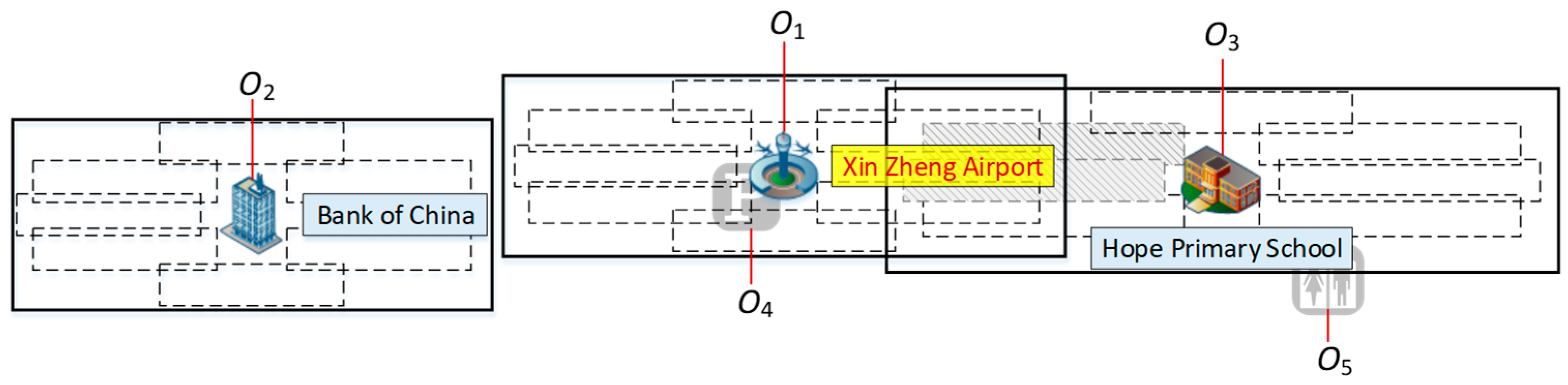Figure 1 visually d.epicts these phenomena—independence, mutual exclusion, and varying degrees of conflict—emerging from spatial disparities among point features during label configuration. Collectively, these phenomena constitute the essential spatial constraints that must be addressed to solve this problem.

In Figure 1, $o_1$ and $o_2$ are independent of each other and are not interfered with by the state selection of the other party, reflecting independence; when $o_1$ selects a certain annotation position, some states of $o_3$ are excluded, and these excluded states are marked by gray areas, showing mutual exclusivity; the state selection of $o_1$ completely prevents $o_4$ from being configured at the same position, which reflects complete blocking, although there is an overlap in the state selection of $o_3$ and $o_5$, the two do not completely exclude each other’s choices, and this phenomenon reflects partial blocking. Through state distribution and area marking, the figure intuitively shows the characteristics of independence, mutual exclusivity, and blocking in the point-feature annotation configuration.

To address the point-feature label placement problem effectively, a precise and computationally tractable mathematical model is indispensable. Our model comprises two core components: (1) the Label Candidate Position Model, which defines the discrete set of possible label locations for each point feature, and (2) the Label Quality Evaluation Function, which quantifies the merit of any given label layout. This section elaborates on these two components and details the specific choices made in this study.

2.1. Label Candidate Position Model

The label candidate position model defines the granularity and structure of the search space, critically influencing both the final optimization outcome and algorithmic efficiency. In the specific context of map label placement, a label is typically modeled as a rectangle, whose width and height are determined by the font, size, and character count of the annotation text. Generating candidate label positions for a point feature, therefore, involves identifying a series of potential placements for this rectangle that do not violate fundamental cartographic norms, such as proximity to the feature and consistent orientation.

Mainstream candidate models can be categorized into sliding models and fixed-position models. Sliding models allow a label to move within a continuous or quasi-continuous space, theoretically enabling better utilization of blank areas. However, this approach drastically increases the dimensionality and continuity of the solution space, leading to an exponential rise in computational complexity. Consequently, this study adopts a fixed-position model.

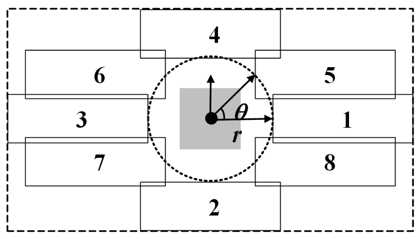
Common fixed-position models include the four-position (top, bottom, left, right) and eight-position (adding the four corners) models. Generally, a larger number of candidate positions increases the model’s potential for exploring the spatial layout. This study employs the multi-level multi-direction candidate position model proposed by Zhou et al. [13], as shown in Figure 2. This model offers flexible control over the number and distribution of candidate positions by adjusting the radius r and angle θ, making it more aligned with cartographic principles and esthetics than traditional models. Balancing label placement quality against algorithmic runtime, our experiments utilize an eight-position variant of this model.

2.2. Label Quality Evaluation Function

An objective and comprehensive quality evaluation function serves as the guiding compass for driving optimization algorithms toward high-quality solutions. Our goal is to obtain the maximum number of clear, esthetically pleasing, and legible conflict-free labels while satisfying all spatial constraints. Drawing upon established cartographic principles [8], we construct a comprehensive label placement quality evaluation function $E(l)$. Its theoretical form is as follows:

$$E(l)=({\omega }_1{\displaystyle \sum _{i=1}^k{E}_1(L_i)+{\omega }_2{\displaystyle \sum _{i=1}^k{E}_2(L_i)+}{\omega }_3{\displaystyle \sum _{i=1}^k{E}_3(L_i)}})/n\times 1000$$

(1)

where $E_1(L_i)$ denotes the label overlap for the i-th point, penalizing conflicts between labels or between a label and important map features. $E_2(L_i)$ represents label position priority, quantifying the desirability of the chosen candidate position relative to its point feature (e.g., a position directly to the right is generally preferred over one directly to the left). $E_3(L_i)$ signifies label–feature association, ensuring a clear visual ownership between a label and the point feature it describes, typically based on the distance between them. ${\omega }_1$, ${\omega }_2$, ${\omega }_3$ are weight coefficients balancing the importance of these optimization objectives. A common setting in the literature [13] is ${\omega }_1=0.5$, ${\omega }_2=0.3$, ${\omega }_3=0.2$.

Treatment of the Association Factor $E_3(L_i)$: Current methods for quantifying association largely rely on computing minute distance differences. However, research in cartography and visual perception indicates that the human eye struggles to effectively discern the ownership relationship when the distance between a label and its point feature is less than approximately 3 pixels [26]. A clear sense of belonging is only affirmed when a perceptible distance difference exists. Therefore, under the standard display and map-reading scales pertinent to this study, the contribution of the association factor $E_3(L_i)$ becomes negligible and unstable. To avoid introducing noise and to simplify the model, we set ${\omega }_3=0$ in our subsequent experimental implementation, effectively disregarding the association term. This means the function we actually optimize is as follows:

$$E(l)={\displaystyle \frac{1000}{n}}\left(0.5\cdot {\displaystyle \sum _{i=1}^k{E}_1(L_i)+}0.3\cdot {\displaystyle \sum _{i=1}^k{E}_2(L_i)}\right)$$

(2)

Consequently, the optimization objective for the point-feature label placement problem is formally defined as follows: to find a feasible label layout configuration L that minimizes the value of the label placement quality evaluation function $E(l)$.

3. Progressive Reinforcement Learning Algorithm Design

3.1. Introduction and Motivation

The point-feature label placement problem presents unique challenges for standard optimization methods, characterized by a high-dimensional discrete action space and stringent spatial constraints. Direct application of general Reinforcement Learning (RL) algorithms suffers from severe inefficiencies: (1) random exploration in the vast action space is largely blind, (2) modeling complex spatial relationships like mutual exclusivity and blocking is not inherent, and (3) policies can prematurely converge to suboptimal solutions.

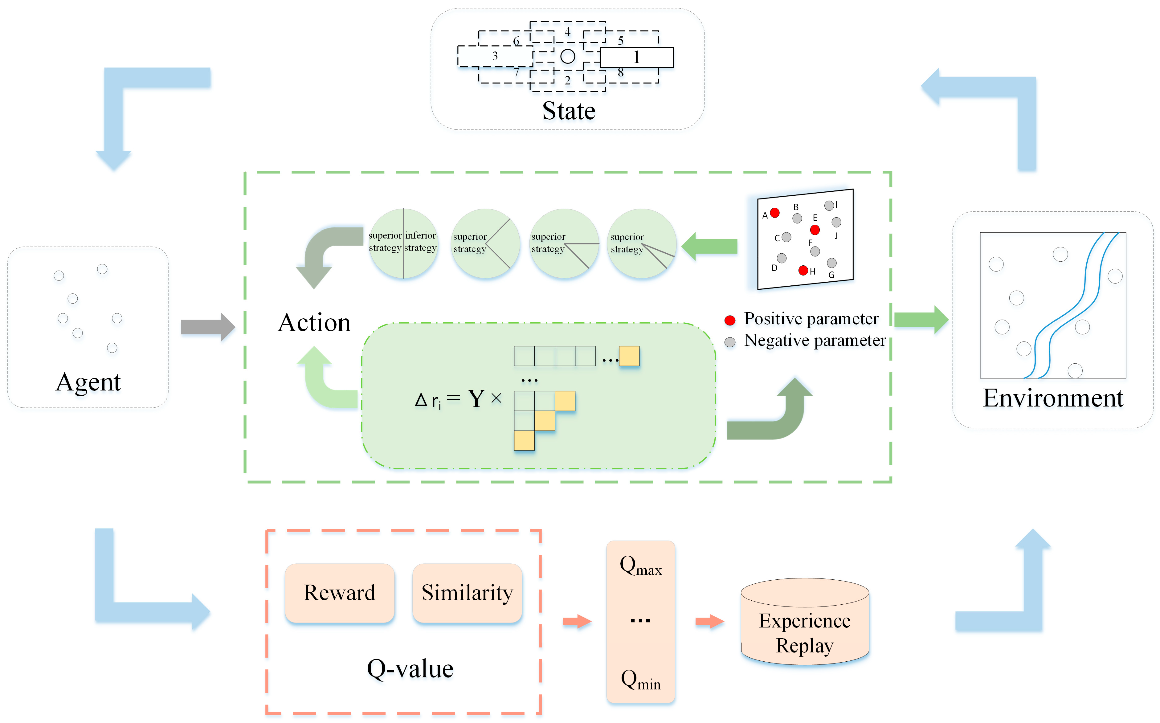
To address these challenges, we propose a Progressive Reinforcement Learning (PRL) algorithm, a framework meticulously customized for the map point-feature label placement problem. The design of PRL revolves around three core pillars: (1) Customized Problem Modeling, (2) Data Mining-Driven Intelligent Action Screening, and (3) Staircase-like policy optimization. The complete workflow of the proposed algorithm is illustrated in Figure 3, which provides a high-level view of the iterative process from initialization to optimal solution output, ensuring a tight coupling with the specific demands of cartographic labeling.

3.2. Customized Problem Formulation: Mapping Label Placement to MDP

To embed the label placement task within the RL paradigm, we establish the following customized mapping:

State (s): The state $s_t$ at iteration is defined as the set of current label positions for all n point features: $s_t=\{l_1^t,l_2^t,\mathrm{\dots },l_n^t\}$, where $l_i^t$ denotes the label position for the point feature $o_i$, selected from its predefined discrete candidate position set $A_i$ (e.g., an eight-position model).

Action (a): An action $a_t$ is defined as selecting a single-point feature of and moving its label to a different position within its candidate set $A_i$. This “single-point adjustment” mechanism is a cornerstone of PRL, decomposing the complex high-dimensional global optimization into a sequence of learnable sequential decisions.

Reward (r): The reward function $r(s_t,a_t,s_{t+1})$ directly reflects the optimization effect of the taken action. It is defined as the negative change in the label quality evaluation function $E(\cdot )$ (formally defined in Section 2.2):

$$r=-[E(s_{t+1})-E(s_t)]$$

(3)

Therefore, maximizing the cumulative reward is equivalent to minimizing the overall label conflict and esthetic deficiency. Crucially, the spatial constraints between labels (mutual exclusivity and blocking) are naturally integrated into the reward signal via the conflict penalty term within $E(\cdot )$, guiding the agent to learn policies that avoid invalid placements.

3.3. Intelligent Action Screening: Data Mining for Targeted Exploration

To overcome the blindness of standard RL exploration, PRL incorporates an Intelligent Action Screening module (corresponding to the module in Figure 3) before each iteration. The core idea is to perform online mining of historical iteration data, thereby identifying “high-value” point features whose adjustment is most critical to the overall layout quality, and prioritizing them for action selection.

We maintain and dynamically update two key metrics for each point feature $o_i$:

Contribution Decline Degree ${\eta }_i(t)$: This counts, over the recent m iterations, how many times an adjustment to the label of $o_i$ resulted in a degradation of the overall layout quality. It identifies points that are “frequently detrimental.”

Contribution Support Degree ${\xi }_i(t)$: This calculates the average magnitude of quality decline across those adjustments that led to degradation. It identifies points whose misplacement, when it occurs, causes “significant harm.”

Based on the pair (${\eta }_i$, ${\xi }_i$), all points are dynamically classified and assigned different selection probabilities:

Active Points (low $\eta$, low $\xi$): Historically beneficial and high adjustment potential. Assigned a high probability of being selected as the action target.

Stubborn Points (high $\eta$, high $\xi$): Historically detrimental and high adjustment risk. Assigned a low probability of selection.

This mechanism transforms random search into directed mining, significantly enhancing exploration efficiency and directly addressing expert concerns regarding “inefficient, random action selection.”

To ensure clear prioritization in screening pre-selected point elements, a “dual-indicator progressive sorting” strategy is adopted to construct an ordered pre-selection set—Primary Sorting: Using the contribution descent degree (${\eta }_i(t)$) as the core metric, sort all point elements in ascending order by ${\eta }_i(t)$. This prioritizes retaining points with “low historical degradation frequency,” ensuring the pre-selection set possesses high optimization potential. Secondary Sorting: If multiple point features have equal ${\eta }_i(t)$ (i.e., ties exist in the primary sorting), use contribution support ${\xi }_i(t)$ as a secondary metric and sort in ascending order by ${\xi }_i(t)$. This sorting prioritizes retaining point features with “low degradation intensity” under the premise of “equal frequency,” further enhancing the quality of the preliminary set.

3.4. Staircase-like Policy Optimization and Q-Learning Update

While the standard allocation mode enhances search efficiency, prolonged reliance on the active interval may cause iterations to converge to local optima, i.e., the optimization is confined to the local space corresponding to the active interval and fails to explore globally superior solutions. To address this issue, a global optimization mode is triggered by a random probability mechanism as a supplement: (1) set a small random probability threshold $p$ (typically $p\ll 1$), and generate a random number $\gamma$ before each iteration; (2) if $\gamma <p$, the global optimization mode is activated, where $M_1$ and $M_2$ represent the number of point features allocated from the stable and stubborn pre-selection intervals, respectively, satisfying $M_1+M_2=M$ (with $M$ denoting the total number of annotation state change point elements selected from the solution space per iteration, and $M_1$, $M_2$ assigned following the same preset proportional constraint as the standard allocation mode); (3) this mode breaks the local spatial constraints by introducing adjustment opportunities for low-potential point elements, explores potentially superior global solutions within the stubborn interval, and thus achieves a balanced trade-off between iterative search efficiency and global optimization performance.

The policy optimization in PRL employs a Q-learning algorithm integrated with a staircase-like policy optimization strategy. The Q-value is updated as follows:

$$Q(s_t,a_t)\leftarrow Q(s_t,a_t)+\alpha [r_t+\gamma \underset{a^{\prime }\in A_{smart}}{\max }Q(s_{t+1},a^{\prime })-Q(s_t,a_t)]$$

(4)

Here, $\alpha$ is the learning rate and $\gamma$ is the discount factor. The key enhancement is that the max operation is performed over the high-quality action subset $A_{smart}$ generated by the Intelligent Action Screening module, rather than the entire action space. This accelerates value propagation.

The “Staircase-like” nature is embodied in the exploration strategy:

The “Staircase-like” nature is embodied in the dynamic adjustment of the exploration rate ϵ within the $\epsilon$-greedy strategy:

$${\epsilon }_t={\epsilon }_0\cdot {(1-{\displaystyle \frac{t}{T_{\max }}})}^{\kappa }$$

(5)

where ${\epsilon }_0$ is the initial exploration rate, tis the current iteration step, $T_{\max }$ is the maximum number of iterations, and $\kappa$ is the decay exponent that controls the curvature of the staircase. This formulation ensures that exploration gradually diminishes in a non-linear, stepwise fashion—mimicking a staircase descent—allowing the agent to shift from broad exploration to focused exploitation as training progresses.

• The training process is divided into multiple cycles, each of length $Y$.
• In the early phase of each cycle, a higher exploration rate $\epsilon$ is set, and actions are primarily chosen from “Active Points,” facilitating broad exploration within promising regions of the solution space.
• In the later phase (low $\epsilon$), action selection relies more heavily on the Q-values, enabling precise exploitation.
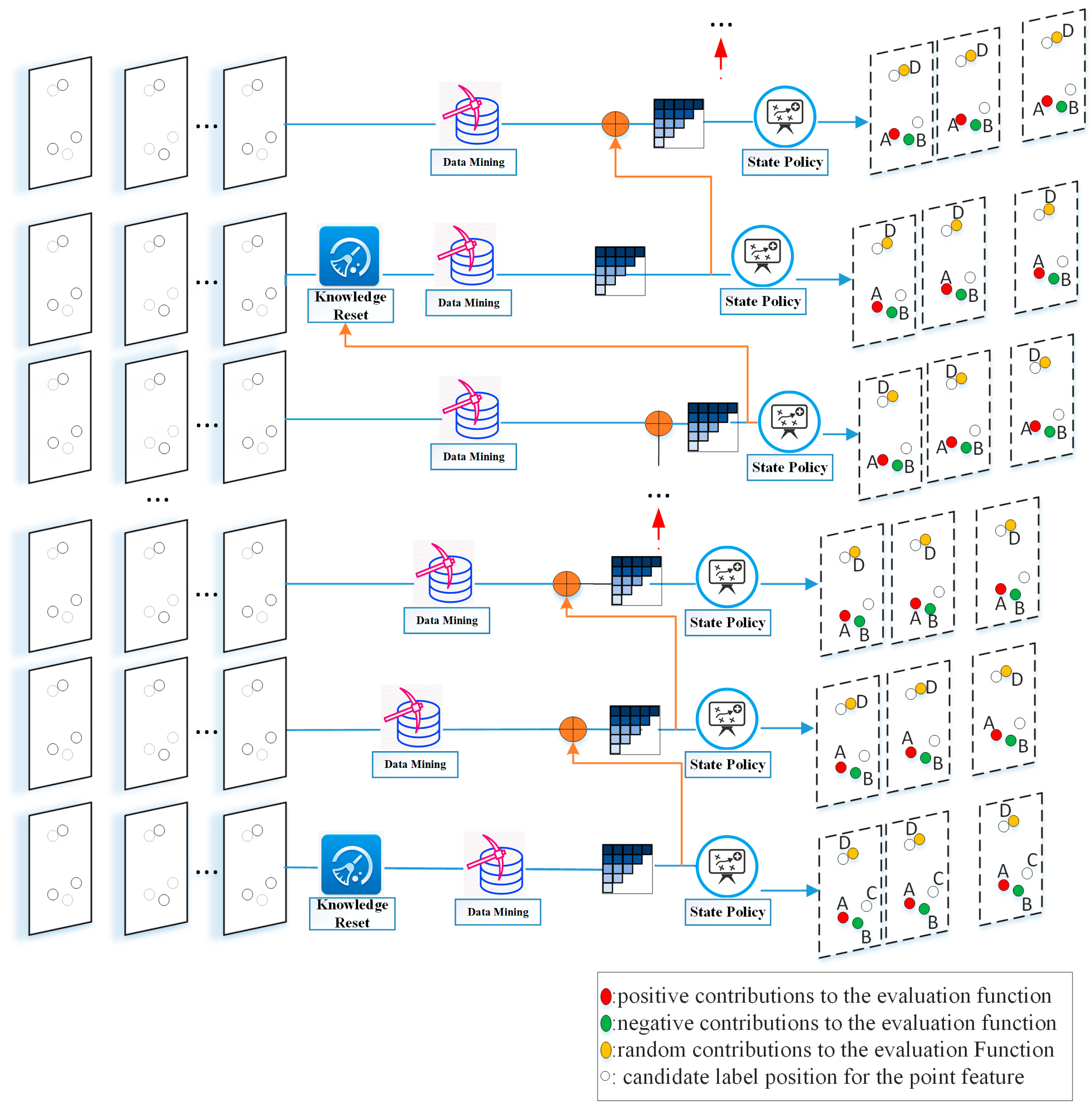
• Upon completion of a cycle, the historical data used to compute ${\eta }_i$ and ${\xi }_i$ for that cycle is cleared (while the Q-table is preserved), and a new cycle begins. This periodic “knowledge reset” prevents interference from stale experience, allowing the algorithm to periodically escape local search patterns and recalibrate its optimization direction.

A schematic representation of the entire stepwise optimization process is presented in Figure 4, which will be elaborated in Section 3.5.

3.5. Algorithm Procedure and Output

Integrating with Figure 6, the complete procedure of the PRL algorithm is as follows:

Initialization: Randomly generate an initial label layout $s_0$, initialize the Q-table, set the cycle length $Y$, and define the maximum number of iterations.

Iterative Loop:

a. State Updating: Update the current state $s_t$ using crossover and mutation in the Genetic Algorithm. The points are selected as active points (low ${\eta }_i$, low ${\xi }_i$) as far as possible, which the current state $s_t$ will be updated in mutation.

b. State Evaluation: Calculate the quality evaluation value $E(s_t)$ for the current state $s_t$.

c. Intelligent Screening: Compute (${\eta }_i$ and ${\xi }_i$) for all points based on recent cycle history, generating the high-probability candidate action set for the current iteration.

d. Action Selection and Execution: Select an action $a_t$ using an $\epsilon$-greedy strategy (biased by the screening results), execute it to obtain the new state $s_{t+1}$ and the reward $r_t$.

e. Policy Update: Update the Q-value using the aforementioned Q-learning formula.

f. Policy Storage: Retain the historically best policy (i.e., label layout) encountered so far.

g. Cycle Management: When the iteration count reaches a multiple of $Y$, reset the cycle’s historical data for ${\eta }_i$ and ${\xi }_i$.

Termination and Output: Upon reaching the maximum iteration limit, output the historically optimal label layout $s^{\ast }$ and its corresponding quality evaluation value.

In summary, the proposed PRL algorithm effectively tackles the optimization challenge of large-scale point-feature label placement through customized MDP modeling, data-driven action screening, and a staircase-like exploration-exploitation mechanism. It ensures high-quality solutions while dramatically improving search efficiency and stability.

4. Experimental Results and Analysis

This section details the experimental study of the Progressive Reinforcement Learning algorithm. To validate the effectiveness and superiority of the Progressive Reinforcement Learning (PRL) algorithm, the experimental design encompasses analysis and comparison from the following perspectives. Section 4.1 describes the detailed experimental setup, including the datasets, parameter configurations, and evaluation metrics. Subsequently, Section 4.2 compares the proposed algorithm with 13 state-of-the-art algorithms. Section 4.3 provides an intuitive, detailed comparison. Finally, Section 4.4 compares the proposed algorithm with the optimized versions of several well-performing algorithms from Section 4.2, analyzing the improvements in label count, quality, and stability achieved by the optimization.

4.1. Experimental Design

4.1.1. Parameter Settings

To validate PRL’s performance on large-scale datasets, we randomly extracted point-feature datasets containing 10,000, 20,000, and 32,312 points from POI data of Kaifeng, Zhengzhou, and Beijing using web crawling technology. As large-scale data typically leads to a slower decline in the objective function value and makes it difficult to fully explore the solution space, we selected these datasets to verify whether the algorithm can achieve satisfactory label configuration results within a limited, yet sufficient, number of iterations. The annotation symbol radius (r) is 5 pixels, the baseline offset distance from the coordinate point to the annotation is 10 pixels, and the annotation font height is 12 pixels. All algorithms in the experiments were implemented in C++ within Microsoft Visual Studio 2010, running on a computer with an Intel (R) Core (TM) i5-8500 3.0 GHz processor and 8 GB of RAM.

The Progressive Reinforcement Learning algorithm (PRL) is compared with Genetic Algorithm (GA), Differential Evolution (DE), Lion Swarm Optimization (LSO), Particle Swarm Optimization (PSO), Tabu Search (TS), Shuffled Frog Leaping Algorithm (SFLA), Simulated Annealing (SA), Sand Cat Swarm Optimization (SCSO), Artificial Bee Colony (ABC), Immune Algorithm (IA), Grey Wolf Optimizer (GWO), Sparrow Search Algorithm (SSA), and Cuckoo Search (CS). During this process, given that the original versions of PSO and DE performed poorly in solving the point-feature annotation problem, we adaptively adjusted their parameters to better align with the problem requirements, seeking optimal solutions. Iteration terminates when the algorithm’s evaluation count reaches a specified number. The evaluation count for all algorithms is set to 420,000. The population size for GA, DE, LSO, PSO, SFLA, SCSO, ABC, IA, GWO, SSA, and CS is set to 100. The parameter settings for all compared algorithms are summarized in

Table 1. Parameters and values used in methods.

Algorithm	Parameters	Parameters Definition	Experimental Value
SA	T0	Initial temperature	40,000
	λ	Annealing speed	0.95
	SAmax	Numbers of Annealing iterations	4000
	Tc	Termination temperature	1.0
	pt	Labeling transformation probability	0.001
GA	pm	Percentage of the elite population	0.2
	Pe	Chromosomal crossover probability	0.8
	pv	Chromosomal mutation probability	0.1
TS	CL	Candidate list scale	0.01
	TL	Tabu list scale	0.05
	FC	Candidate list frequency	5
	FT	Tabu list frequency	5
CS	TMax	Maximum number of iterations	4200
	pa	Egg found probability	0.9
	α	Step control value	1.0
GWO	TMax	Maximum number of iterations	4200
	wα	Weight of Alpha wolf	0.5
	wβ	Weight of Beta wolf	0.3
	wδ	Weight of Delta wolf	0.2
DE1	Pe	Chromosomal crossover probability	0.8
	pv	Chromosomal mutation probability	0.1
	F	DE mutation scaling factor	0.5
DE2	pDE	Weight of DE	0.7
	pGA	Weight of GA	0.3
	F	DE variation probability	0.5
	Cr	DE hybridization probability	0.8
	CGA	Genetic mutation probability	0.1
SSA	TMax	Maximum number of iterations	4200
	λP	Producer scale	0.2
	λS	Scrounger scale	0.5
	ST	Safety value	0.8
SFLA	TMax	Maximum number of iterations	4200
	m	Memeplexes size	10
	n	Frogs’ number of each memeplex	10
	N	Infection steps number between two consecutive shuffling in a memeplex	10
PSO1 PSO2	TMax	Maximum number of iterations	4200
	Vmax	Initial particle velocity	6.0
	ω	Inertia weight	0.9
	c1	Individual acceleration coefficient	2.0
	c2	Social acceleration coefficient	1.0
	ωmin	Minimize inertia weight	0.4
SCSO	TMax	Maximum number of iterations	4200
	SM	Initial hearing sensitivity of sand cats	2.0
ABC	TMax	Maximum number of iterations	4200
	SN	Number of employed bees and onlooker bees	100
	L	Scout bee activation threshold	200
	pb	Detection probability	0.5
LSO	TMax	Maximum number of iterations	4200
	β	Percentage of adult lions in the pride factor	0.2
PRL	N	Number of agents	100
	TMax	Maximum number of iterations	4200
	Pe	Crossover probability of object variables	0.8
	pv	Mutation probability of object variables	0.1
	λa	Percentage of active object	0.001
	Y	Length of the progressive training process	10

.

Optimization configuration problems typically pursue both rapid solution improvement in the short term (fast descent speed) and robust long-term search capability (effective exploration when time is not the primary constraint). Considering that in many high-dimensional complex discrete problems, time requirements are not the foremost consideration, this paper focuses on search capability assessment as the core research objective, setting the iteration experiment at 420,000 evaluations.

4.1.2. Comparison Between Reinforcement Learning Algorithm and Other Algorithms

PRL is compared with commonly used optimization algorithms, primarily evaluating the label count and label placement quality under different annotation densities (5–40%). The experiments are conducted on three datasets of different scales: 10,000, 20,000, and 32,312 points. The median result of 10 independent runs for each algorithm is recorded to ensure the reliability and stability of the results.

4.1.3. Algorithmic Detail Comparison

Under the high annotation density scenario of 40%, the performance of PRL in complex datasets is validated by comparing the detailed distribution of conflict-free annotation points. Analyzing the detailed results of label count and placement quality further demonstrates PRL’s advantages in local optimization and global search capability.

4.1.4. Strategy Optimization Comparison

To verify the performance of the enhanced Reinforcement Learning algorithm (PRL) after incorporating the stepwise strategy optimization, this study compares it with the optimized versions of several well-performing algorithms from Section 4.2. The experiment particularly focuses on analyzing the improvement in label count, quality, and stability of the enhanced algorithms under the condition of high annotation density (40%) on the large-scale dataset (32,312 points). Annotation density is a crucial metric for measuring dataset complexity. Higher annotation density implies increased complexity of the problem space, a significant rise in the number of local optima traps, and higher demands on the algorithm’s global search and local exploitation capabilities. Therefore, conducting experiments under a 40% annotation density allows for a more comprehensive examination of each algorithm’s global exploration ability, local optimization capability, and performance differences in complex problems. Box plots and statistical analysis are used to assess the role and effect of the stepwise strategy optimization in enhancing the algorithm’s global search and local exploitation capabilities.

4.2. Comparison Between the Stepwise Reinforcement Learning Algorithm and Other Algorithms

To validate the effectiveness of the algorithm proposed in this paper, PRL is compared with GA, DE, LSO, PSO, TS, SFLA, SA, SCSO, ABC, IA, GWO, SSA, and CS. Comparisons are conducted under eight commonly used annotation densities (ρ): 5%, 10%, 15%, 20%, 25%, 30%, 35%, and 40%. Annotation density refers to the ratio of the sum of the areas occupied by map symbols and their labels to the total map area, reflecting the distribution density of features and annotations. The comparison primarily focuses on label count and the label quality evaluation function. For statistical reliability, each algorithm was independently run 10 times. 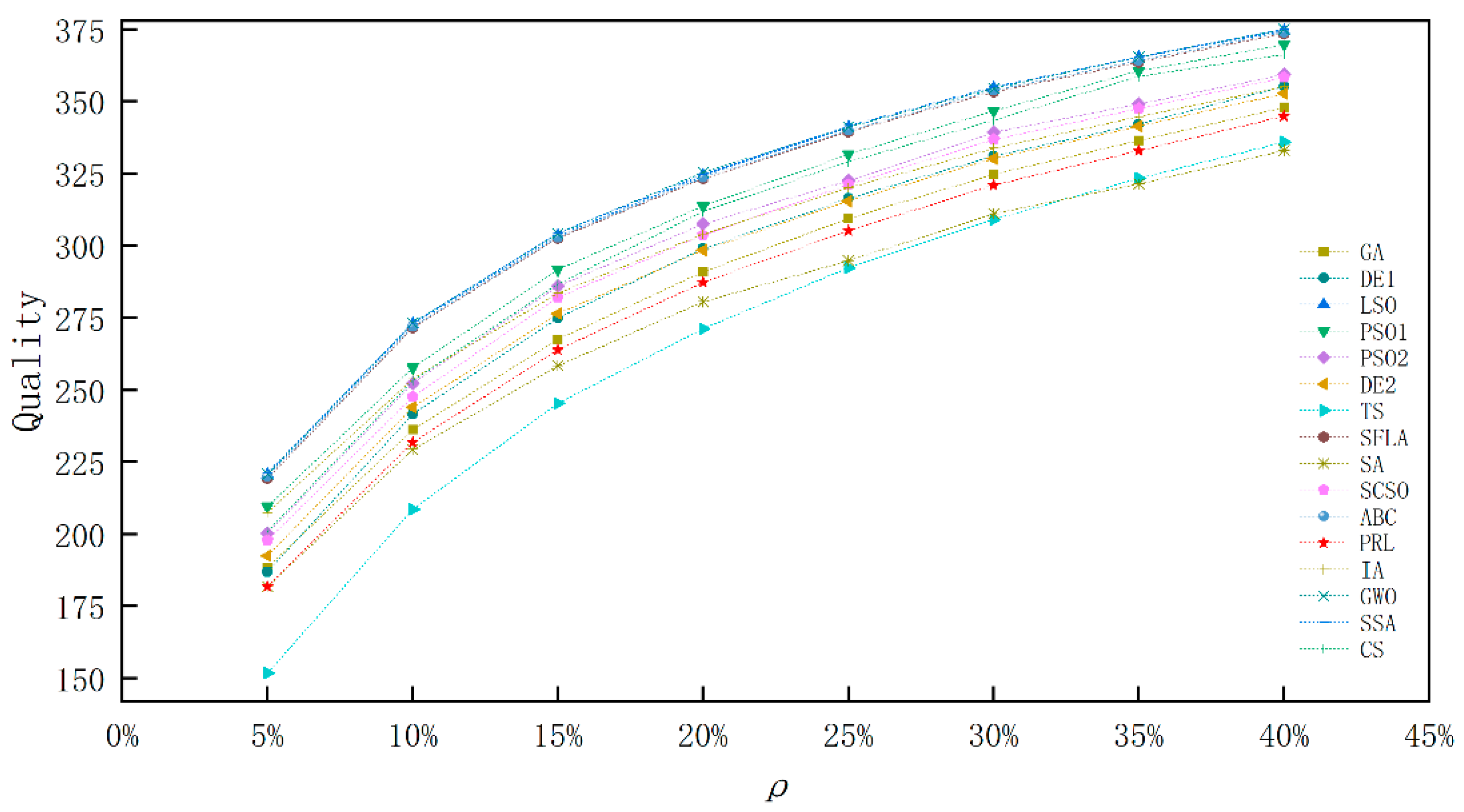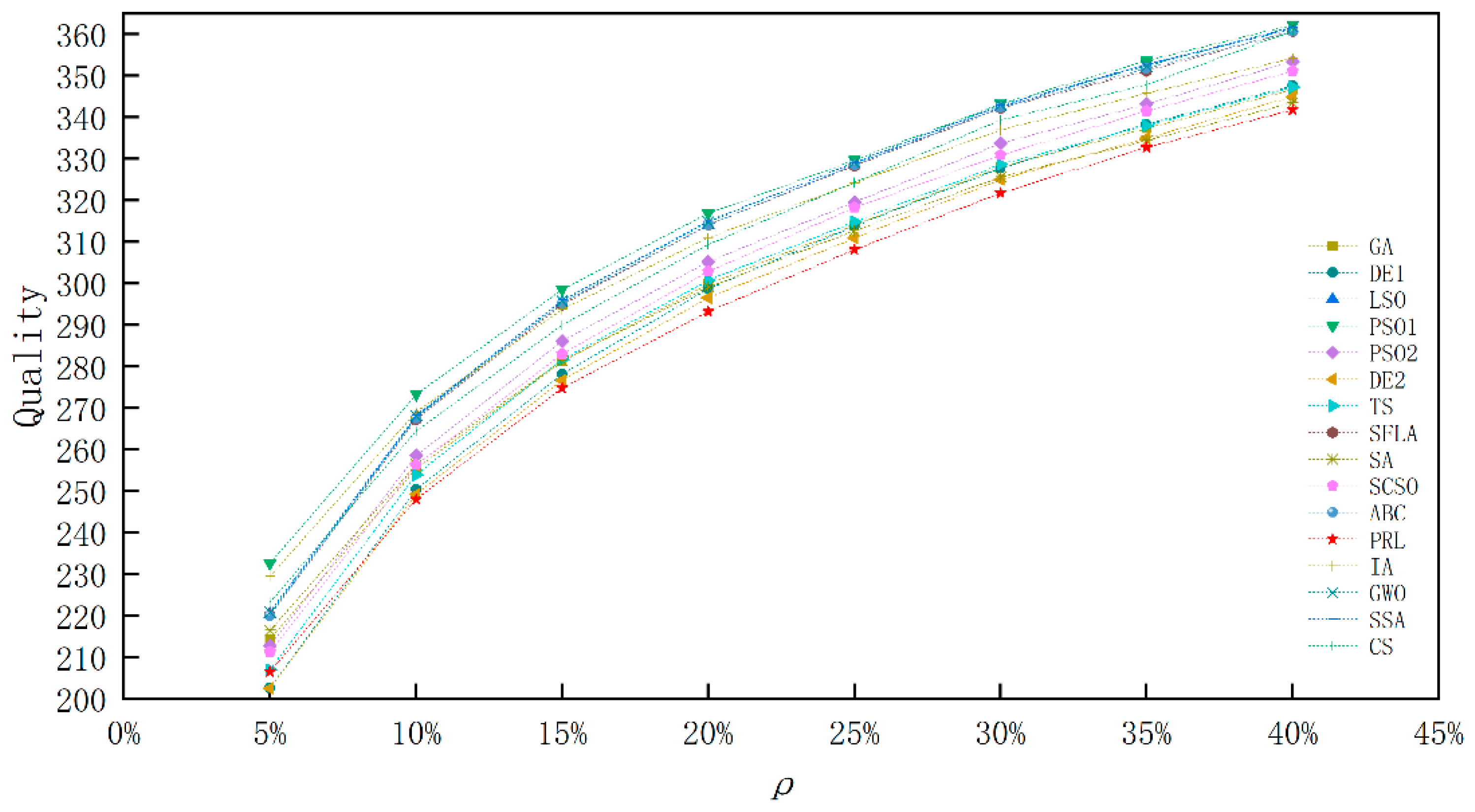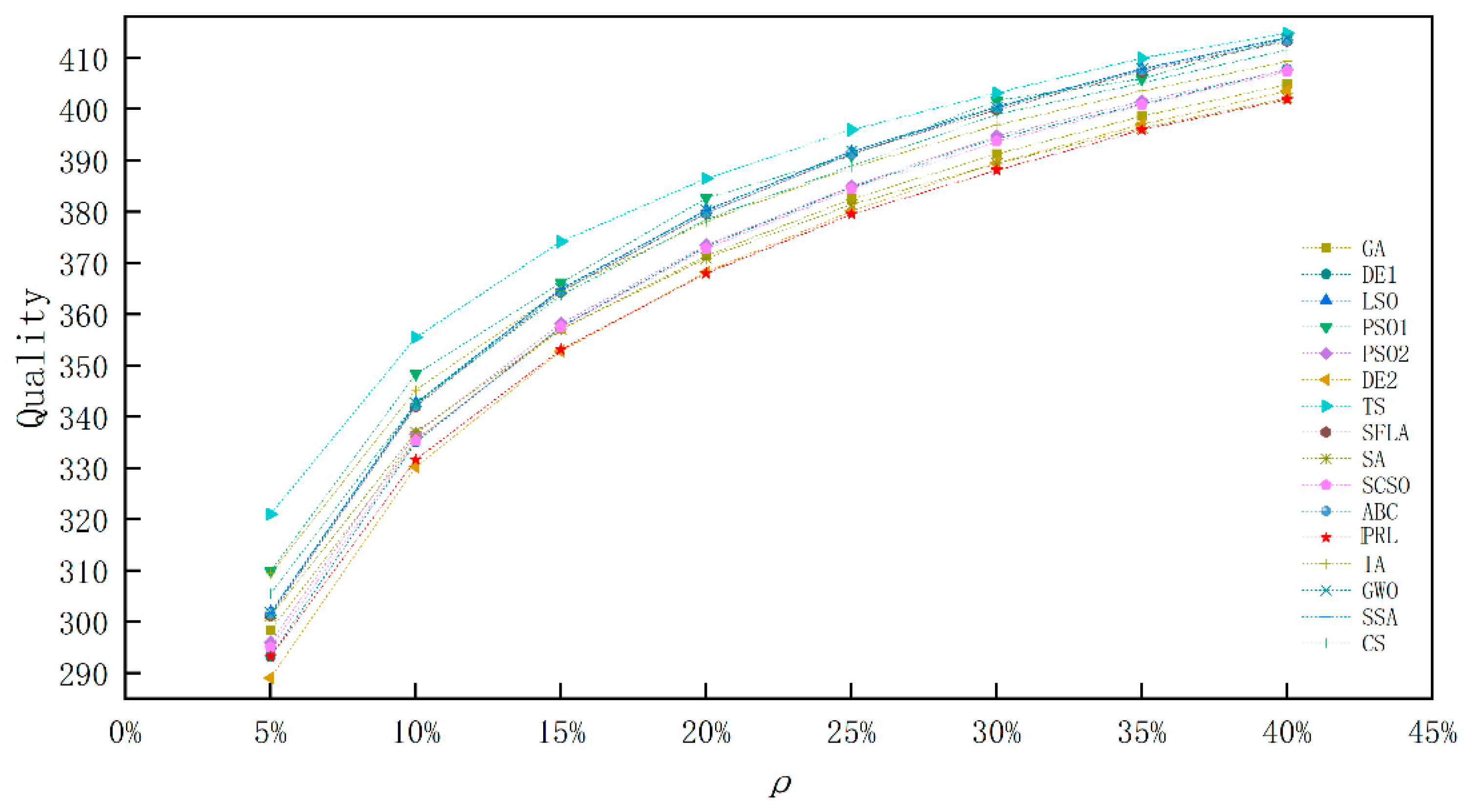Figure 5, Figure 6 and Figure 7 show the comparison of the median label quality for PRL versus GA, DE, LSO, PSO, TS, SFLA, SA, SCSO, ABC, IA, GWO, SSA, and CS under 5–40% annotation density. The median represents the performance value for the majority of the 10 runs of each algorithm, providing a measure of central tendency.

Figure 5, Figure 6 and Figure 7 display the comparison of the median label quality between PRL and other algorithms on the 10,000, 20,000, and 32,312-point datasets under different annotation densities. A smaller evaluation function value indicates a better labeling result. For the 20,000 and 32,312-point cases, the label quality evaluation function value of PRL is significantly smaller than that of GA, DE, LSO, PSO, SFLA, SCSO, ABC, IA, GWO, SSA, and CS, achieving better labeling results. On the 10,000-point dataset, the label quality of PRL is slightly inferior to that of TS and SA. This is because, in a dataset of this scale, exhaustive search becomes relatively difficult, leading TS and SA to demonstrate superior label quality in the initial iterations. However, if the number of iterations is further increased, TS and SA might be influenced by label placement priorities and become trapped in local optima, whereas PRL, due to its dynamic learning capability, can progressively optimize the global layout, and its final label quality is expected to surpass that of TS and SA. Furthermore, on the 32,312-point dataset with 5% annotation density, PRL’s label quality result is worse than that of DE2. This is because DE2 employs a differential formula for its mutation operator, which allows it to place outliers in the optimal annotation priority positions, thereby obtaining better results.

In summary, PRL demonstrates strong global search capability when processing large-scale data. Its algorithmic structure and optimization mechanism make it more likely to find the global optimum in complex search spaces and less susceptible to being trapped in local optima.

4.3. Detailed Comparison Between the Stepwise Reinforcement Learning Algorithm and Other Algorithms

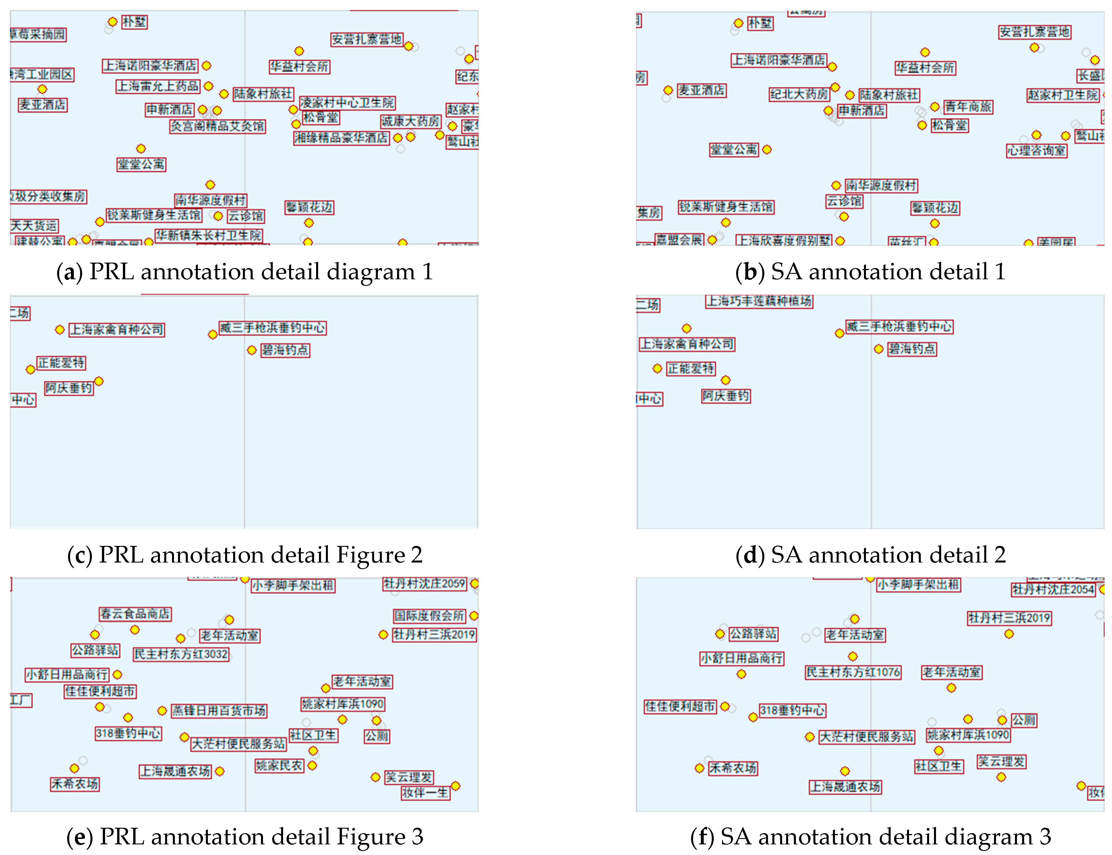
This section selects the SA algorithm, which performed best in Section 4.2, for a detailed comparative analysis. Figure 8 shows the detailed comparison between PRL and SA under 40% annotation density on the 32,312-point dataset. The figure displays only conflict-free point features and their labels. As can be seen, in detail image 1, PRL and SA annotated 26 and 22 conflict-free point features, respectively. In detail image 3, they annotated 22 and 18 conflict-free point features, respectively. PRL’s label count is clearly superior to SA’s, indicating that PRL performs more outstandingly in labeling results. In detail image 2, although both PRL and SA annotated five conflict-free point features, PRL’s label quality is higher, further proving PRL’s superiority in complex scenarios.

4.4. Comparison of Different Algorithms Based on Dataset Order Guidance via Data Mining [15]

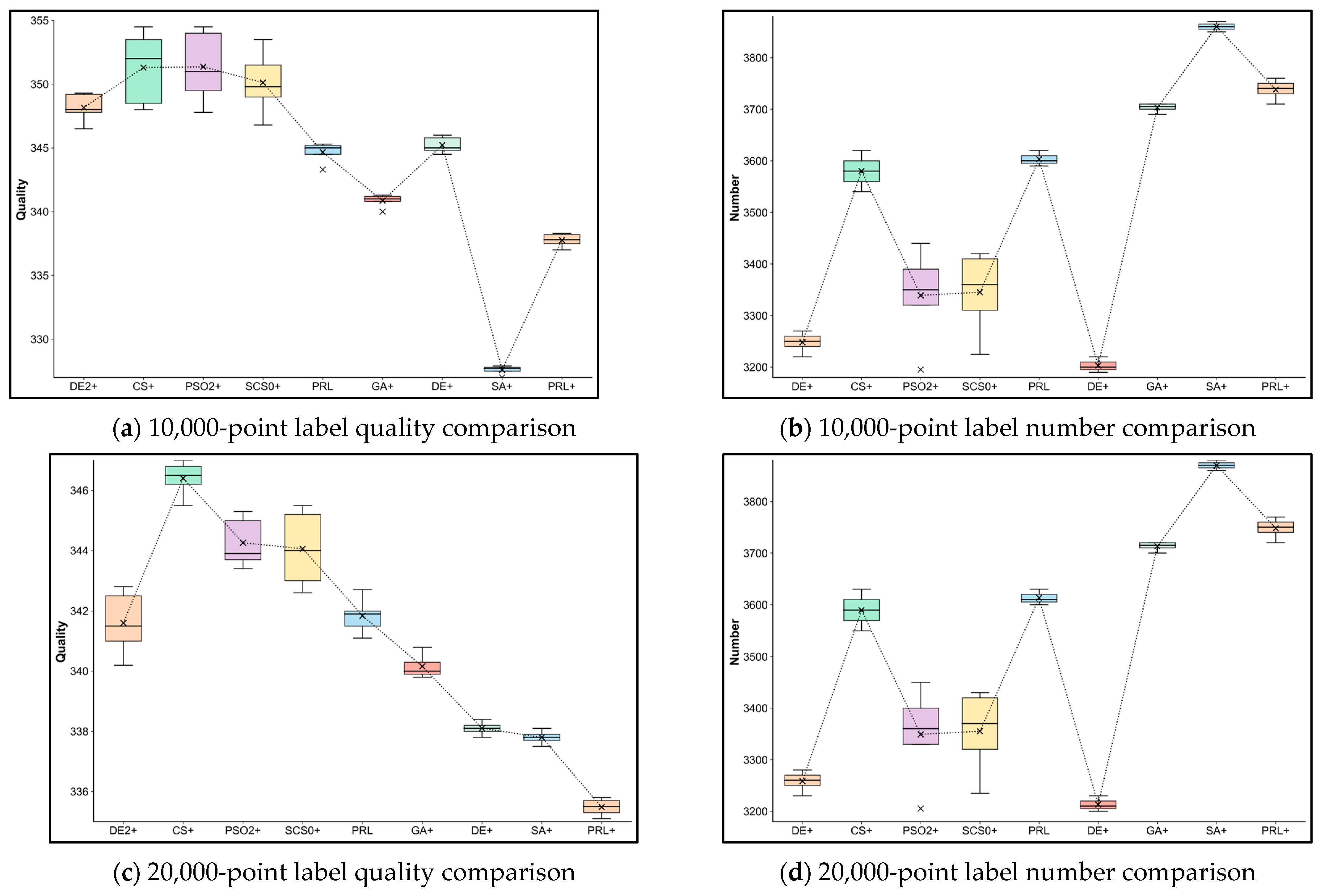
According to the description in Section 3.4, we introduced an action screening mechanism based on stepwise learning and improved the Reinforcement Learning algorithm. 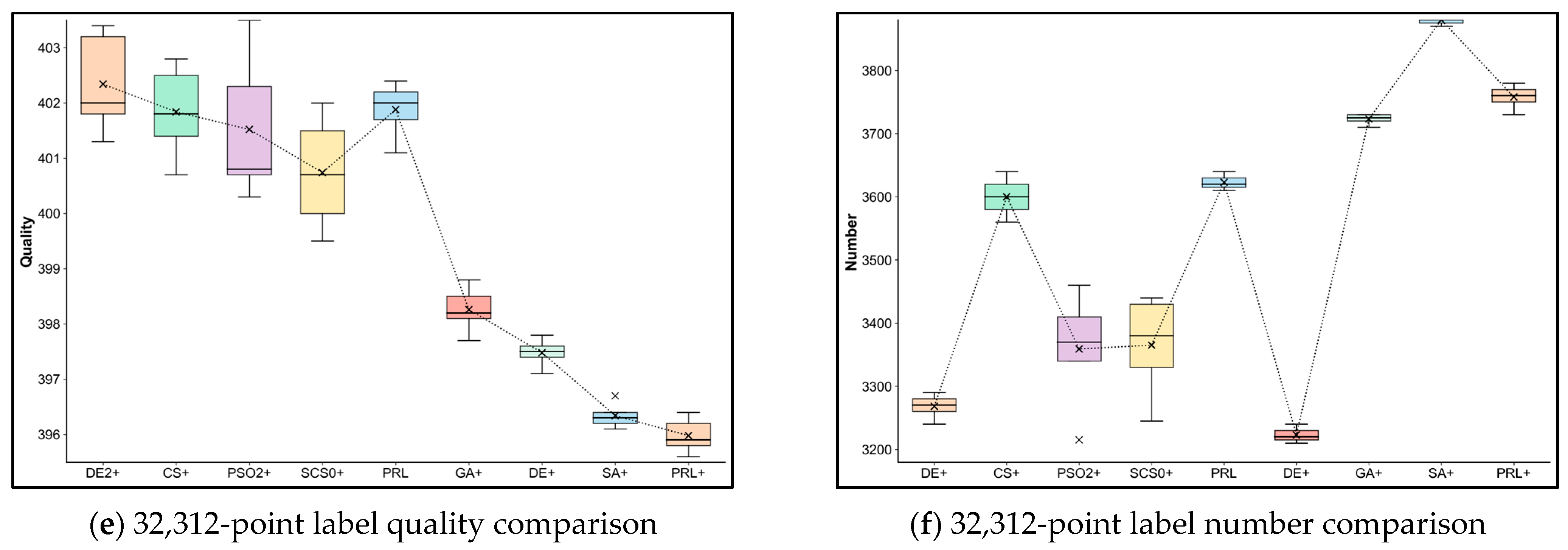To further verify the algorithm’s performance, we selected the well-performing swarm intelligence and heuristic algorithms from Section 3.5 and conducted statistical experiments based on the dataset spatial data mining from reference [15]. This includes DE2+, CS+, PSO2+, SCSO+, RL, GA+, DE+, SA+, and PRL+. Subsequently, a comparative experimental analysis was performed on datasets of different scales under the most complex condition of 40% annotation density.

Stepwise strategy optimization dynamically adjusts the algorithm’s learning rate, enabling it to gradually adapt to changes in task complexity, thereby significantly enhancing its optimization capability. The experimental results are presented in the form of box plots, showcasing the performance distribution of different algorithms in terms of label quality and quantity. This provides a comprehensive assessment of the average performance and stability of each algorithm, clearly demonstrating the effectiveness and superiority of the improvement strategy in complex optimization tasks.

The experimental results show that all optimized algorithms exhibit high competitiveness. On the 10,000-point dataset, the label quality of the PRL+ algorithm is second only to that of SA+. Swarm intelligence algorithms like PSO2+ and SCSO+, although showing improved optimization capability, still fall short of SA+ and PRL+ in local search within complex environments. This is because, on small-scale datasets, heuristic algorithms (e.g., GA+, DE+, SA+) retain an advantage in local optimization capability. While PRL+ shows slight insufficiency in fully exploring the search space for small-scale problems, its stability and average performance remain excellent. As the dataset scale increases to 20,000 points, the performance of the PRL+ algorithm surpasses all others, demonstrating significant optimization effectiveness and strong robustness. This indicates that its stepwise learning strategy significantly enhances global search ability and can effectively balance exploration and exploitation. In contrast, although the median performance of SA+ is relatively close, its distribution is slightly more dispersed, and its optimization stability is somewhat inferior. When the scale is further extended to 32,312 points, PRL (Optimized Version) continues to exhibit excellent global search capability and significantly widens the gap with other algorithms. On this dataset, the fitness value distribution of PSO2+ and SCSO+ is broader, indicating greater fluctuation in their optimization performance and difficulty in adapting to the complexity of ultra-large-scale problems, as show in Figure 9.

In conclusion, the experimental results demonstrate that the optimized PRL+, based on the stepwise learning strategy, performs excellently in complex environments and on large-scale problems. On the 10,000-point dataset, PRL+ ranks second in label quality, but on the 20,000-point and 32,312-point datasets, PRL+ demonstrates its powerful global search capability and optimization potential with the best performance. This result further proves the significant advantage of combining Reinforcement Learning with stepwise optimization strategies for highly complex problems, making it an effective method for handling complex scenarios and large-scale datasets.

5. Conclusions

This paper addresses large-scale, high-density point-feature label placement with a customized Progressive Reinforcement Learning (PRL) algorithm, motivated by limitations of existing metaheuristic methods (premature convergence, inefficient random search, and poor spatial constraint modeling).

Framed as a sequential decision-making framework, PRL’s core innovations include a staircase-like policy optimization strategy (transitioning from exploration to exploitation) and a data mining-driven Intelligent Action Screening (IAS) mechanism. The latter uses “Contribution Decline Degree” and “Contribution Support Degree” to prioritize adjustments to “high-value” points, converting blind stochastic search into directed, data-informed optimization.

Experiments on real-world POI datasets (up to 32,312 points) show PRL outperforms 13 state-of-the-art methods (e.g., Simulated Annealing, Genetic Algorithm, and POPMUSIC) in label layout quality and conflict-free placement count, demonstrating strong robustness, adaptability, and efficiency for dense cartographic labeling.

Despite these advantages, several limitations of the current PRL framework should be acknowledged. First, the method is currently tailored for static point-feature label placement and has not been extended to dynamic or streaming map data, where label positions or point features may evolve over time. Second, it primarily handles rectangular labels with uniform size, lacking explicit handling of heterogeneous label geometries and dimensions (e.g., circular or irregularly shaped labels with varying aspect ratios). Third, while efficient for the tested datasets, the computational cost may escalate under extremely large iteration budgets or ultra-high-density scenarios, as the sequential decision-making process inherently incurs additional overhead compared to lightweight heuristic methods. Finally, the generalization of the framework beyond the specific task of point-feature label placement—such as line or area feature annotation—remains to be fully explored, as the current reward function and action space are tightly coupled to the constraints of point-based labeling.

Future research will focus on extending this framework to incorporate more complex cartographic rules, adapting it for dynamic or streaming data scenarios, and exploring its integration with deep learning models for even more intelligent spatial configuration tasks.