Ionospheric Scintillation Anomalies from COSMIC-2 GNSS-RO from 2019 and 2024 as Potential Earthquake Precursors

Abstract

Currently, there are no consistent earthquake precursors for early warning. However, the correlation between earthquakes and ionospheric scintillation, measured using the S₄ index via GNSS-RO, is under active study. This research analyzes S₄ anomalies as a potential earthquake proxy, using GNSS-RO data from COSMIC-2/TGRS (Tri-GNSS Radio Occultation System) collected from 2019 to 2024. It examines over 71,000 global earthquakes within ±60° of the equator with magnitudes greater than 4. The quality of S₄ anomalies has been enhanced by filtering out space-weather-induced disturbances using the daily planetary geomagnetic index (Kp) and the solar activity flag collected from ground stations. The S₄ anomalies were calculated using robust statistical methods, such as the standard deviation and the interquartile range. This study evaluated the correlation with a confusion matrix, a receiver operating characteristic curve, and various figures of merit. The results demonstrated a promising positive S₄ anomaly between 1 and 7 days before the analyzed earthquakes, indicating the potential of ionospheric scintillation as an earthquake precursor, with the robust statistical methods employed instilling confidence in the validity of our findings.

1. Introduction

Ionospheric scintillations (ISs) are rapid fluctuations in the amplitude and phase of signals caused by scattering from small-plasma-density irregularities in the ionosphere and modulated by solar radiation, geomagnetic activity, and, in some cases, geophysical processes related to lithospheric stress [1,2,3].

Several studies have examined ISs linked to seismic activity that appears before earthquakes, due to the piezoelectric effect arising from the geological stress-induced compression of rocks [4]. This effect generates fluctuating electric and magnetic fields, resulting in ionospheric disturbances [5]. Despite extensive research, no consistent method exists for predicting earthquake occurrences [6]. As an alternative, seismic risk forecasting provides probabilistic estimates of future earthquakes based on location, magnitude, and frequency [7].

Recent studies have investigated the relationship between IS and earthquake activity using Global Navigation Satellite System Reflectometry (GNSS-R) [8,9,10] and GNSS Radio Occultation (GNSS-RO) [11] data. All of them have indicated that anomalies in the S₄ index could be potential precursors to seismic events. GNSS-RO data from FORMOSAT-7/COSMIC-2 detected intensity scintillations before earthquakes in the Coral Sea in 2022 [12]. Similarly, GNSS reflectometry (GNSS-R) data from NASA’s CYGNSS mission demonstrated correlations between ionospheric disturbances and seismic activity over oceanic regions [8]. Additional results support this hypothesis, including pre-seismic ionospheric anomalies identified before the 2016 Kumamoto earthquake [13] and the 2019 Laiwui earthquake [14], in which GPS and CSES satellite data confirmed ionospheric perturbations preceding the events [15]. Furthermore, volcanic activity has also been linked to ionospheric fluctuations, as observed during the 2021 La Palma eruption, where GNSS-RO and GNSS-R data recorded significant ionospheric variations [11].

Total Electron Content (TEC) anomalies in GNSS-RO data have further strengthened the hypothesis that pre-seismic ionospheric plasma fluctuations could indicate impending earthquakes [16,17]. However, distinguishing earthquake-induced disturbances from other space-weather phenomena remains challenging, necessitating further research that integrates TEC, plasma parameters, and geomagnetic data to enhance prediction models [18].

In [19], a new approach was presented for the automated classification of ionospheric disturbances in the lower atmosphere. This technique leverages GNSS-RO data from Spire’s CubeSats constellation, combining signal processing with semi-supervised machine learning, and implements spectral clustering within a wavelet-based metric framework. These methods enhance global monitoring of ionospheric anomalies associated with seismic events.

In addition, geomagnetic field disturbances observed from space have been increasingly investigated as potential earthquake precursors. Measurements from the European Space Agency’s Swarm satellite constellation have revealed statistically significant anomalies in the magnetic field and total electron content before several moderate-to-large earthquakes. These IS are commonly interpreted within the lithosphere–atmosphere–ionosphere coupling (LAIC) framework [20]. Recent Swarm-based studies have demonstrated that integrating magnetic field observations with ionospheric parameters can improve the physical interpretation of pre-seismic signals and strengthen multiparametric approaches for earthquake precursor analysis [21,22].

Numerous additional studies have associated earthquake occurrences with various geophysical parameters, such as land surface temperature [23,24], surface latent heat flux [25], outgoing longwave radiation [26], geomagnetic and electric fields [27,28], and Schumann resonance [29,30].

This research explores pre-earthquake IS anomalies using advanced data analytics, image processing, and anomaly-detection techniques to identify potential links to future seismic activity. The ionospheric intensity scintillation index (S₄ parameter) observed from 2019 to 2024 has been analyzed to indicate IS fluctuations. ISs are detectable in GNSS-RO data when the reflected signal remains coherent at the tangent point [3].

Over 71,000 earthquakes with magnitudes (M_w) ≥ 4, within ±60° latitude, have been examined. Confusion matrices and Receiver Operating Characteristic (ROC) curves have been utilized to assess the effectiveness of S₄ anomalies as indicators of seismic activity. Using the Standard Deviation (STD) and Interquartile Range (IQR) methods, S₄ anomalies were identified and analyzed in the temporal datasets of the 71,000 earthquakes with M_w ≥ 4.

To minimize diurnal variations caused by solar activity, a nighttime filter (00:00–06:00 LT) was applied to S₄ data. This filter is crucial because it helps isolate IS anomalies from background noise, thereby improving the accuracy of the analysis. However, some residual scintillations from diurnal activity may persist [31]. Filtered and aggregated S₄ data were then processed, and daily S₄ anomalies were calculated for each 1° × 1° grid cell.

The key contributions of this study are as follows: (1) A comprehensive approach to processing and filtering S₄ data, including projection onto the tangent point, nighttime filtering, and quality control. (2) Applying robust anomaly detection techniques, such as confusion matrices and ROC curves, to optimize detection thresholds. (3) A large-scale analysis of over 71,000 earthquakes from 2019 to 2024, ensuring statistically significant results. (4) Optimized threshold testing: A systematic assessment of various detection thresholds to identify the most reliable correlation framework. (5) A comprehensive correlation analysis: A classified evaluation examining the effects of depth, elevation, magnitude, land cover, latitude, and earthquake type. These improvements contribute to the expanding field of ionospheric seismology, reinforcing the potential of IS anomalies as precursors to seismic activity, while addressing challenges posed by space-weather interference and minimizing signal noise.

This paper is organized as follows: Section 2 discusses the materials and methods for ingesting, processing, and analyzing S₄ anomalies, including the input data and statistics of the ocean earthquakes studied. Section 3 presents the results, followed by a discussion in Section 4. Lastly, Section 5 summarizes the conclusions.

2. Materials and Methods

This section describes the processes for acquiring, processing, and calculating S₄ anomalies from COSMIC-2 GNSS-RO data.

2.1. Overview of Data Collection and Processing Architecture

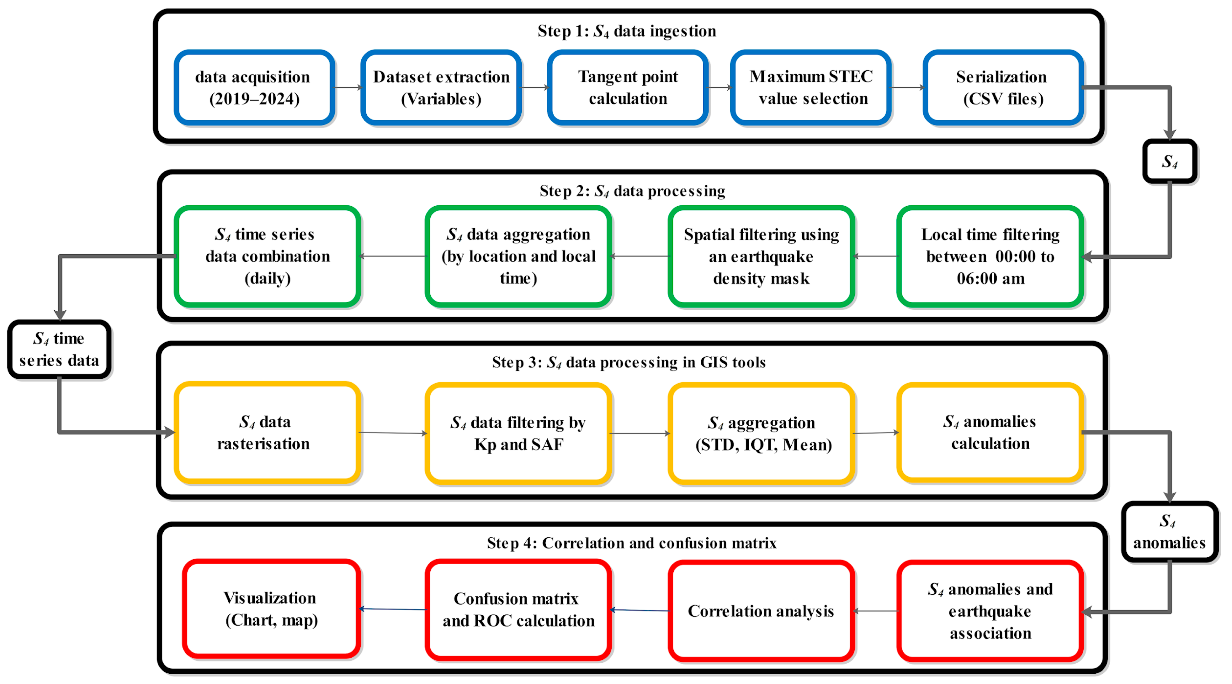
The flowchart outlines the steps involved in S₄ data analysis and earthquake association, divided into four main stages, as explained in Figure 1.

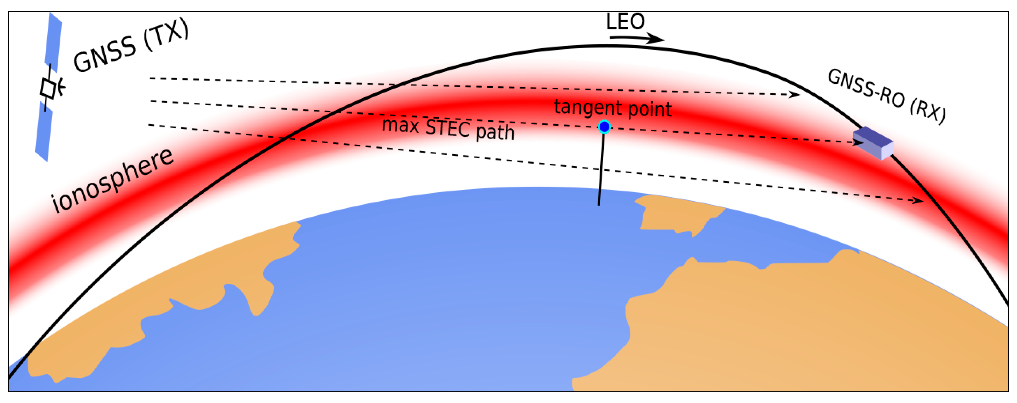
Step 1 (Blue Section): S₄ data ingestion starts with acquiring data from 2019 to 2024. This is followed by extracting relevant variables using the SAT-ETL-Integrator software Version 1 [32] in a distributed way [33] in the “Calcula” platform [34] and calculating tangent points using GPS and Low-Earth-Orbit (LEO) satellite positions from COSMIC-2, utilizing methods cited in [35] and [36], as illustrated in Figure 2.

The pierce points in the occultation path’s profile data must demonstrate a Slant TEC value of at least 80% of the maximum STEC within that profile, as specified in [11] and [37]. This filter increases the likelihood of detecting ionospheric points prone to scintillation, whereas an elevation ≤ 0° indicates an occultation involving rays that traverse the ionosphere. Lastly, the dataset is serialized into CSV files for additional processing [38].

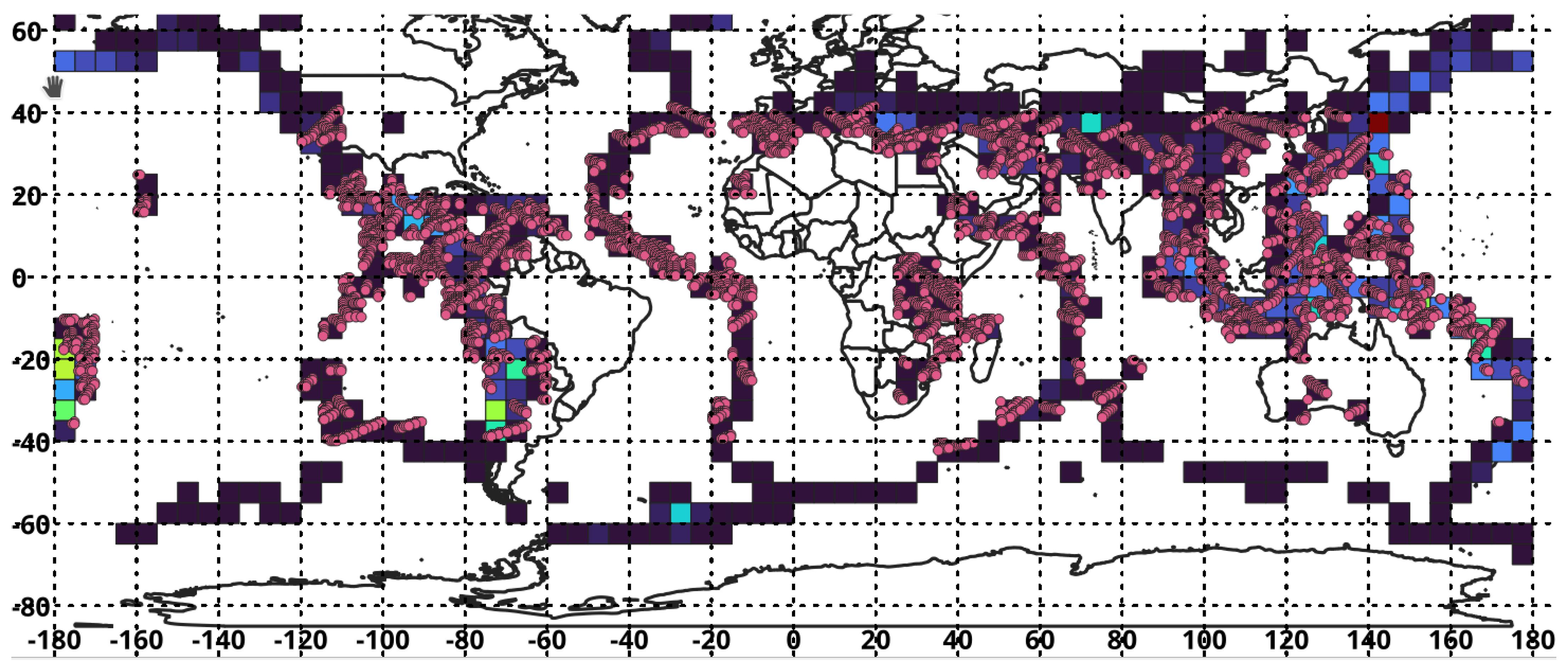
Step 2 (Green Section): The S₄ data processing stage includes daily aggregation of S₄ time series data by location and local time. A time filter from 00:00 to 06:00 AM has been applied to retain only nighttime datasets, which are less influenced by solar activity. Figure 3 depicts the global distribution of filtered data points, represented as pinpoints aligned with the earthquake frequency mask from 2019 to 2024, with squares indicating seismic zones, faults, and tectonic plate boundaries. This distribution highlights the relationship between earthquake-prone regions and ionospheric variations, which is crucial for studying seismic–ionospheric interactions.

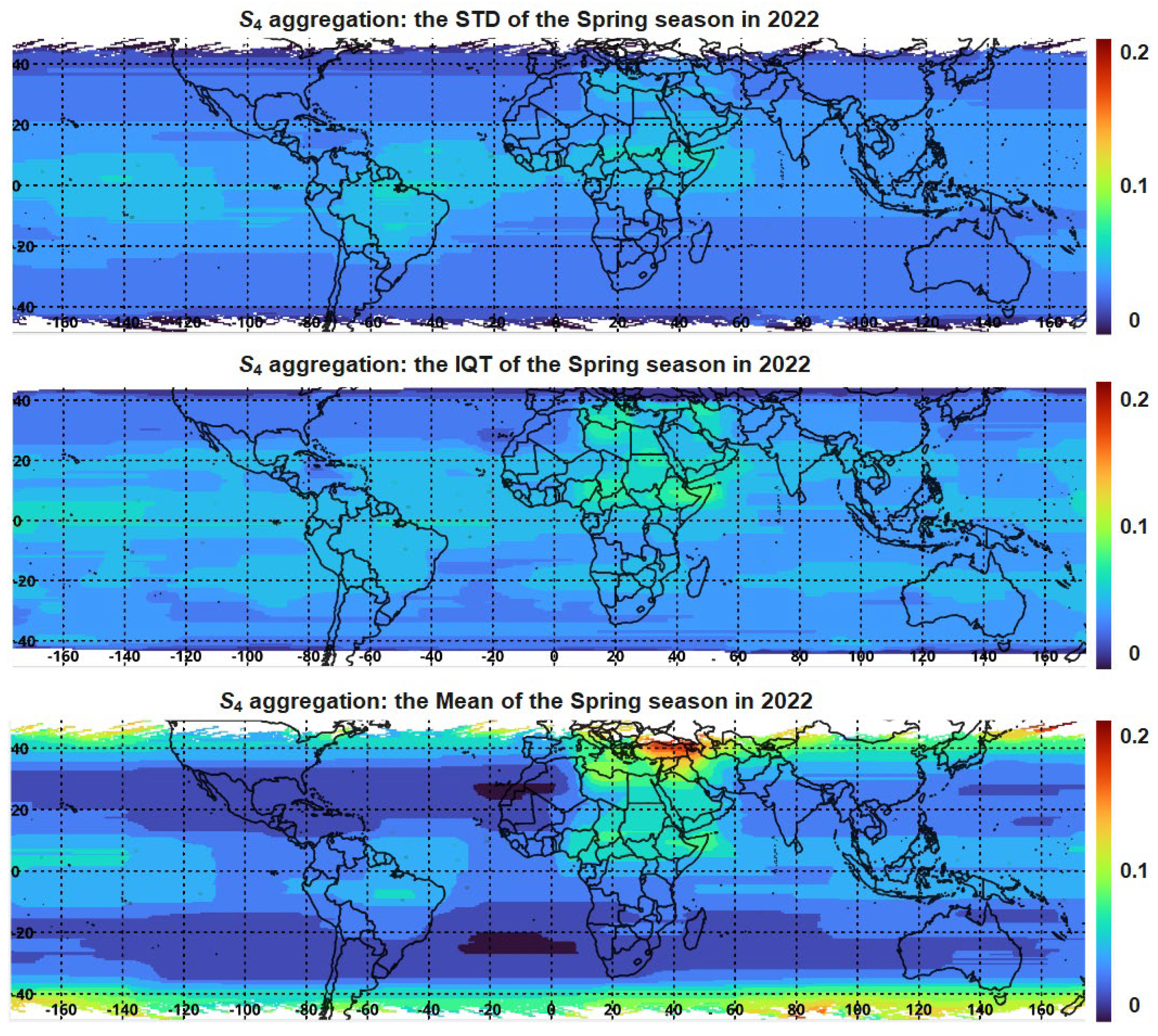
Step 3 (Yellow Section): S₄ data processing in Geographic Information System (GIS) tools includes rasterizing S₄ data, applying the Kp index and solar activity filters, and calculating STD and IQR for each season of every year for anomaly detection. Figure 4 shows the S₄ STD, IQR, and Mean aggregation maps for the Spring season of 2022, highlighting spatial variations in ionospheric irregularities. The color scale ranges from 0 (blue) to 0.2 (red), indicating the intensity of fluctuations across various regions.

The S₄ aggregation maps were generated by S₄ daily observations within a 1° × 1° geographic grid cell. These daily values were then seasonally aggregated for each year. For each grid cell and season, the mean, STD, and IQR of the S₄ time series were computed, resulting in the spatial maps shown in Figure 4. The top map shows the STD, revealing minor variations across latitudes, with slightly elevated values near high-latitude areas. The middle map shows the IQR, with a similar pattern: lower variability near the equator and greater variability at mid-latitudes. The bottom map displays the Mean S₄ values, showing a small concentration of IS in the northern hemisphere, particularly at higher latitudes.

Overall, the S₄ values remain relatively low (<0.2) across most regions, suggesting stable seasonal ionospheric conditions. These results emphasize that IS activity is more prevalent at higher latitudes. The consistent patterns across the three metrics confirm the seasonal and regional dependencies of ionospheric variability. Finally, these aggregated S₄ maps will be used to compute S₄ anomalies for each day.

In this research, S₄ deviation values exceeding C multiplied by the STD of S₄ are identified as anomalies, as shown in Equation (1). The coefficient range was chosen to include common anomaly-detection thresholds, such as robust IQR-based fences and sensitivity levels used in statistical thresholding, enabling ROC-based optimization. Tested C values of 0.5, 0.7, 1, 1.5, 2, and 2.5 span a wide sensitivity range in ionospheric and space-weather studies.

Lower C detects weak signals; higher C reduces false alarms but may miss subtle signals, allowing assessment of the trade-off between detection and false alarms. Values satisfying the criteria in Equation (1) were identified as S₄ anomalies in the time series. The IQR method provides an alternative way to estimate a dataset’s statistical distribution using quartiles. The IQR is defined as the difference between the 75th percentile (Q3) and the 25th percentile (Q1): IQR = Q₃ − Q₁. As with the previous method, the same six values of C have been evaluated. Following Equation 2, S₄ anomalies are defined as values that exceed C times the IQR. To identify anomalous IS events, two complementary statistical methods were used: the STD and the IQR methods. The STD-based approach assumes that background S₄ variations are approximately Gaussian, enabling anomalies to be detected as significant deviations from the mean. In contrast, the IQR method is a robust, non-parametric estimator based on quartiles and is less sensitive to outliers and non-Gaussian behavior, which are common in ionospheric time series.

|S₄(t) − μS₄| ≥ C · STD

(1)

|S₄(t) − μS₄| ≥ C · IQR

(2)

Here, S₄(t) denotes the scintillation index at time t, μS₄ is the seasonal mean value, STD is the standard deviation, and IQR = Q₃ − Q₁ represents the interquartile range derived from the 75th and 25th percentiles. The coefficient C controls the detection sensitivity and was systematically varied to optimize anomaly discrimination.

In this study, “anomaly” means a deviation from the local seasonal background within each (1° × 1°) grid cell, not just the occurrence of scintillation. Persistent equatorial and auroral scintillation are considered climatology, and only departures above the baseline are anomalies. Therefore, the association with earthquakes is considered probabilistic and regional, rather than evidence of a global ionospheric change caused by individual seismic events.

Step 4 (Red Section): Correlation and Confusion Matrix analysis connects S₄ anomalies with earthquake occurrences, evaluating their potential as seismic precursors [39]. This methodology ensures a systematic approach to processing, analyzing, and validating S₄ ionospheric anomalies for earthquake forecasting.

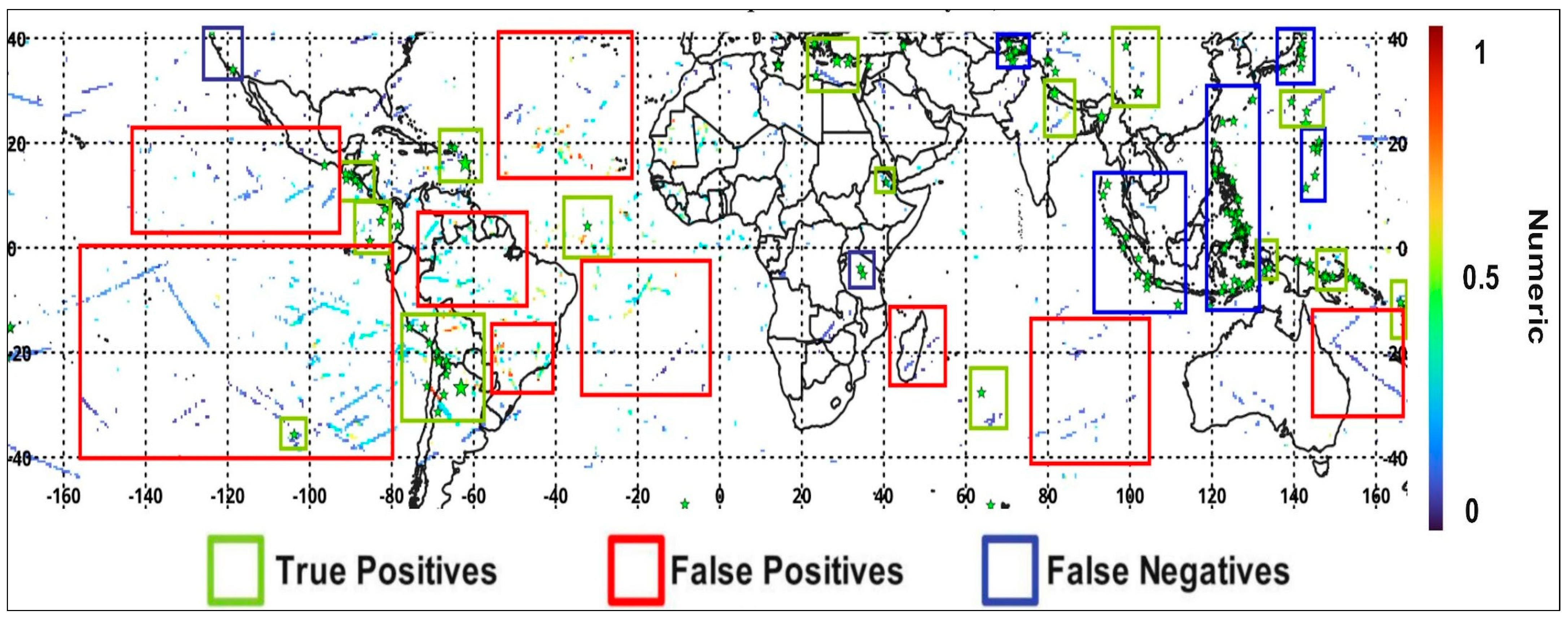
This study builds on previous works but utilizes different input data and updated spatial and temporal filtering conditions [6]. Following the methodology outlined in our earlier paper, we have reapplied the spatio-temporal aggregation of S₄ anomalies and earthquake occurrences [40]; Figure 5 shows the spatiotemporal association between S₄ anomalies and earthquake occurrences on 18-01-2023. The COSMIC-2 S₄ data confusion matrix has been recomputed using the same equations described in our prior publication [8].

The validation metrics shown in

Table 1. Details of the evaluation metrics and their formulas.

Metric	Formula
Total Positives (CP)	CP = TP + FN
Total Negatives (CN)	CN = FP + TN
Prevalence	CP/(CP + CN)
True Positive Rate (TPR)	TP/(TP + FN)
False Negative Rate (FNR)	FN/(TP + FN)
False Positive Rate (FPR)	FP/(FP + TN)
True Negative Rate (TNR)	TN/(FP + TN)
Accuracy (ACC)	(TP + TN)/(CP + CN)
Positive Likelihood Ratio (LR+)	TPR/FPR
Negative Likelihood Ratio (LR−)	FNR/TNR
G-mean	$\sqrt{(TPR\times TNR)}$
Diagnostic Odds Ratio (DOR)	(TP × TN)/(FP × FN)
Chi-square statistic	χ2 = [T (TP × TN − FP × FN)2]/[(TP + FP)(TP + FN)(TN + FP)(TN + FN)] Where $T=TP+FP+FN+TN$
p-value	p = 1 − Fχ2(χ2, df = 1) Where $F_{{\chi }^2}$ is the cumulative distribution function of the chi-square distribution with 1 degree of freedom.
95% Confidence Interval of DOR	exp[ln(DOR) ± 1.96 × $\sqrt{(1/TP+1/FP+1/FN+1/TN)}$]
Area Under Curve (AUC)	Σ [(FPRi − FPRi−1)(TPRi + TPRi−1)]/2
Euclidean ROC Distance	d = $\sqrt{[{FPR}^2+{(1-TPR)}^2]}$

and the confusion matrix definition have been used to quantify the extent to which detected scintillation anomalies are associated with earthquakes. We use a space–time matching rule and a confusion-matrix formulation. An earthquake is considered “matched” if at least one anomaly is detected within a spatial radius of r km from its epicenter and within a temporal window of Dt days relative to the earthquake origin time. Using this rule, we define the confusion-matrix as follows:

• True Positives (TPs): anomalies that occur within (r, Dt) of an earthquake.
• False Positives (FPs): anomalies not matched to any earthquake within (r, Dt);
• False Negatives (FNs): earthquakes for which no anomaly is detected within (r, Dt);
• True Negatives (TNs): non-event space–time intervals with no anomaly and no earthquake occurrence.

The performance metrics shown in Table 1 are systematically evaluated across earthquake categories to assess how well S₄ anomalies distinguish themselves from random events, providing an objective measure of their statistical significance.

The influence of earthquakes on the surrounding geophysical environment is commonly calculated using empirical relationships linking the moment magnitude to spatial and depth-related quantities. The spatial extent of seismic influence is often approximated by a strain radius R, which scales with M_w according to

R = 10^{0.43 Mw}

(3)

where M_w denotes the moment magnitude, this relationship provides an estimate of the region over which stress accumulation and associated electromagnetic, and ionospheric effects may be detectable.

2.2. Data Sources

This section presents the data used, notably COSMIC-2, the Geomagnetic Field, the Solar Activity Indicator, and the earthquake database.

2.2.1. S₄ Data from COSMIC-2 Mission

GNSS-RO is a method for atmospheric and ionospheric sounding that measures variations in GNSS satellite signals using radio-occultation techniques [41]. Different surface-reflected signals in GNSS-R and GNSS-RO rays traverse the ionosphere tangentially as GNSS satellites rise or set relative to a receiver onboard an LEO satellite. This method eliminates ground-reflection disturbances, enabling consistent studies across land and oceanic regions. As explained in Figure 1 the GNSS-RO technique, in which a GNSS satellite (Tx) transmits signals that traverse the ionosphere and reach a LEO satellite (Rx) [11]. The tangent point, where the signal path is closest to Earth, represents the maximum Slant TEC region, which is crucial for ionospheric studies. This study utilizes open-access data from COSMIC-2 (FORMOSAT-7) [42].

COSMIC-2 comprises six LEO mini-satellites (300 kg each) launched on 25 June 2019, and it has a 24° inclination orbit [43]. The dataset employed, Level 1b podTC2, provides the essential information to calculate the tangent point in the ray trajectory closest to Earth using GPS and LEO satellite positions. Each tangent point corresponds to an S₄ scintillation index value, which reflects ionospheric irregularities [44]. While COSMIC-2 provides GNSS and LEO coordinates for each occultation event, it does not offer a direct reference coordinate for determining the precise S₄ location. This study leverages the available data to analyze ionospheric disturbances and their correlation with GNSS-RO observations. Only the variables required for S₄ computation, tangent point localization, and quality control were retained to ensure a concise, application-focused dataset description.

2.2.2. Geomagnetic Field and Solar Activity Indicator (GFZ Ground Stations)

Geomagnetic field and solar activity flag data from GFZ provide insights into the effects of space weather on the ionosphere [45]. These datasets include geomagnetic indices such as Kp and Dst, and solar activity parameters such as the F10.7 flux, which help identify IS and TEC fluctuations caused by geomagnetic and solar storms [46].

Integrating these flags with GNSS-RO data enhances understanding of ionospheric variability during extreme solar events [47]. This study uses the planetary Kp index, calculated as a biased average of K indices from 13 mid-latitude geomagnetic stations. The Kp index ranges from 0 to 9, where 0 indicates minimal geomagnetic activity, and 9 signifies an extreme geomagnetic storm. The SAF monitors the daily intensity of solar radiation.

Solar activity and geomagnetic disturbances strongly influence ionospheric variability and can produce scintillation levels comparable to or exceeding those from seismic activity. During solar or geomagnetic storms, background ionospheric fluctuations may hide weaker pre-seismic signals. To minimize this masking, periods of high geomagnetic and solar activity, indicated by the Kp index and solar activity flag, were excluded from the analysis.

2.2.3. Earthquake Datasets from USGS Seismic Stations

The earthquake datasets from the United States Geological Survey (USGS) seismic stations provide real-time and historical records of seismic activity worldwide. These datasets include earthquake magnitude, depth, location, and time, offering essential information about tectonic events [48]. In this study, 71,000 earthquakes with M_w ≥ 4 have been examined, but only 12 are presented as examples to clarify the methodology.

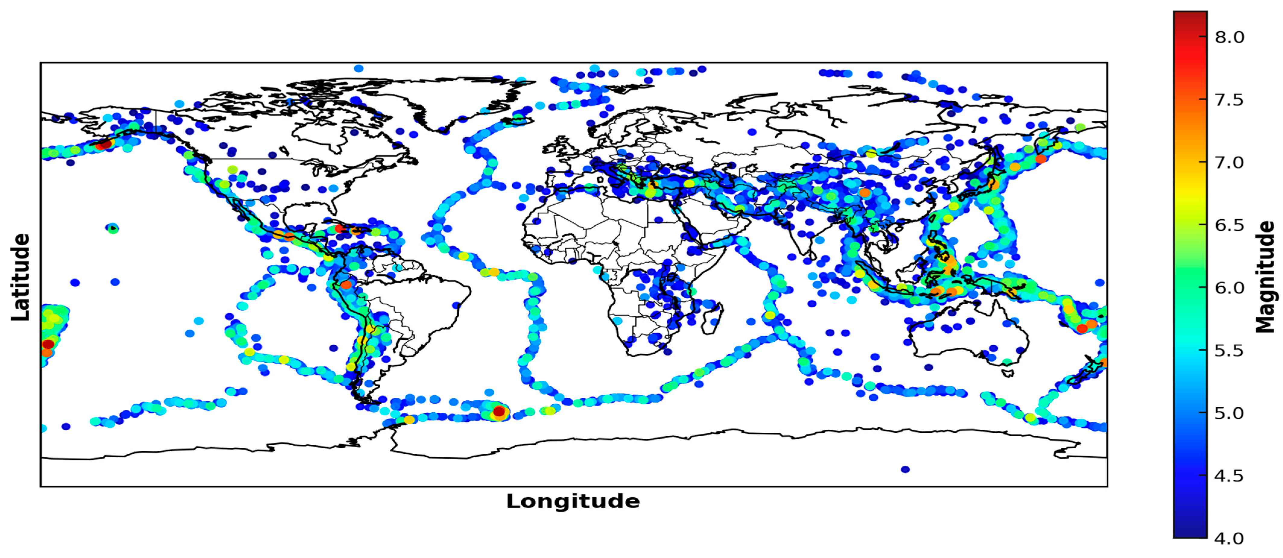
Figure 6 shows the geographical distribution of earthquakes between 2019 and 2024, revealing a strong correlation between seismic activity and tectonic plate boundaries [49]. The color gradient represents earthquake magnitudes, ranging from 4.0 (dark blue) to above 8.0 (red), with most events occurring in the Pacific Ring of Fire, the Himalayan belt, and the Middle East. Japan, Indonesia, and South America are known for the strongest earthquakes (M_w ≥ 7).

Transform faults, such as the San Andreas Fault, produce strike-slip earthquakes with significant surface rupture, while deep-focus megathrust events (M_w ≥ 7) dominate subduction zones. Intraplate earthquakes, though less frequent, occur in continental interiors due to crustal deformation and the reactivation of ancient faults. M_w ≥ 7 concentrates along subduction boundaries, emphasizing the importance of plate movements in seismic activity and the need for hazard preparedness [50].

Table 2. Details on the classification of M_w, depth, and altitude.

Mw		Depth		Region
Classes	Range (Mw)	Classes	Range (km)	Classes	Latitude (°)
7	≥7	DP0	0–20	NEM	(+21°)–(+60°)
6	6–6.9	DP1	21–50	EQT	(−20°)–(+20°)
5	5–5.9	DP2	51–100	SEM	(−21°)–(−60°)
4	4–4.9	DP3	101–400
		DP4	>400

classifies earthquakes by magnitude, depth, and geographic region to enable systematic analysis of seismic events. M_w are grouped into four classes (≥7, 6–6.9, 5–5.9, 4–4.9), while depth ranges from shallow (0–20 km, DP0) to very deep (>400 km, DP4). Regions are categorized by latitude: NEM (+21° to +60°), EQT (−20° to +20°), and SEM (−21° to −60°), encompassing global seismic activity zones. This classification aids in understanding earthquake distribution, risk assessment, and tectonic influences across various regions.

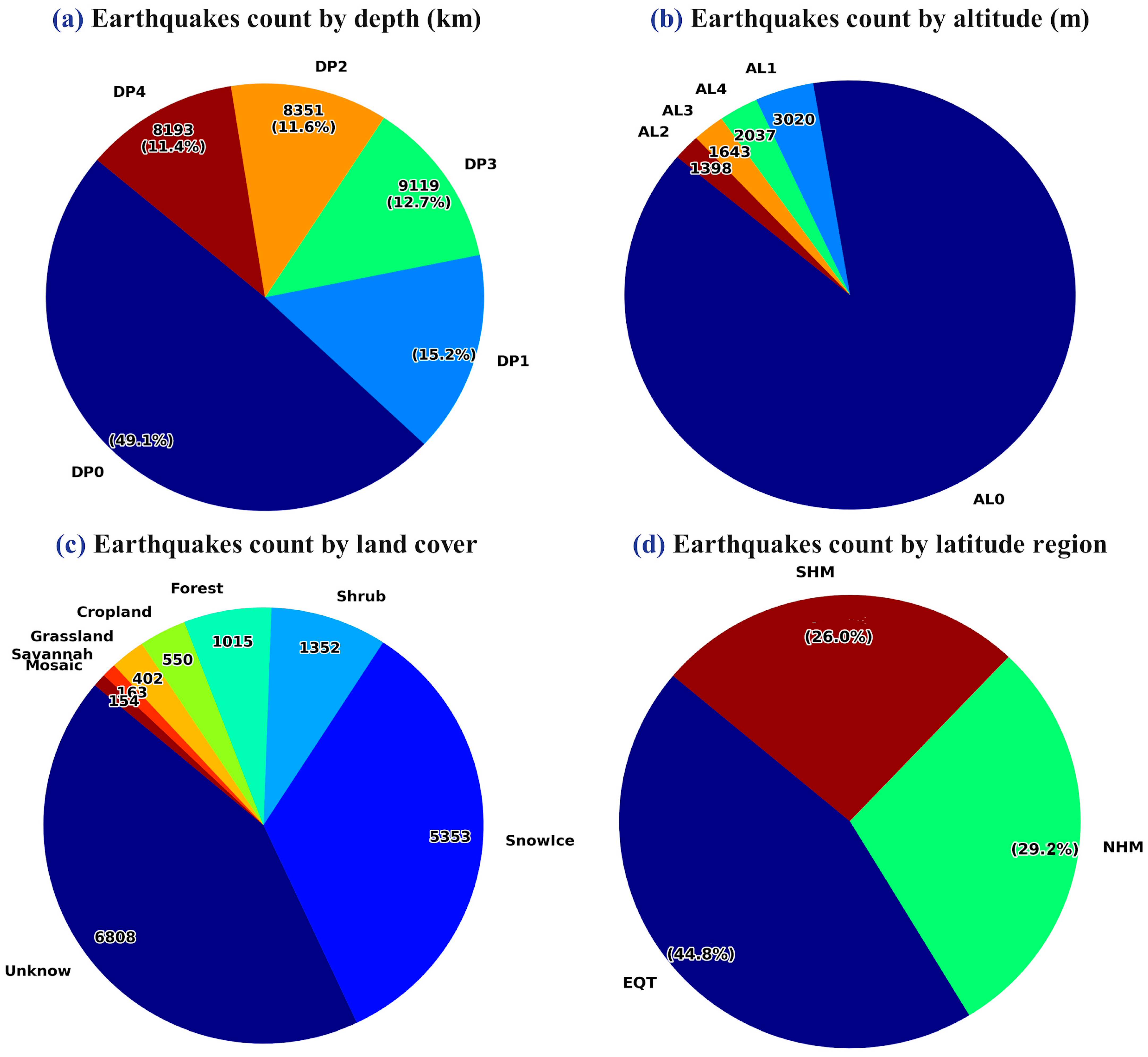
Figure 7 provides a statistical overview of earthquake occurrences based on M_w, depth, altitude, land cover, and type. The pie chart (a) shows that nearly 49.1% (35,264 earthquakes) occurred at shallow depths (DP0, 0–10 km), while only 11.4% (8193 events) reached DP4 (deep-focus earthquakes).

Concerning altitude (chart b), most earthquakes (37.3%, 3021 events) occurred at low altitudes (AL1), while high-altitude regions (AL3–AL4) account for 45.5% of events. Land cover analysis (chart c) indicates that 6808 earthquakes occurred in unclassified land cover, followed by 5353 in snow/ice regions, with the fewest in grassland (402 events) and cropland (550 events). Lastly, earthquake classification (chart d) confirms that 99% (71,163 events) are tectonic, while only 1% (700 events) are volcanic, highlighting the dominance of fault-related seismic activity. These statistics emphasize the impact of tectonic characteristics, depth, and environmental factors on earthquake distribution and forecasting factors.

3. Results

After data-quality, nighttime, and Kp/SAF filtering, 71,872 earthquakes with sufficient S₄ (M_w ≥ 4) coverage remained and were evaluated using the same space–time association rule. ROC curves are complemented by hypothesis testing (chi-square p-values) to explicitly demonstrate the statistical significance of the observed association. Different confusion matrices, stratified by M_w, depth, altitude, land cover, and earthquake type, have been analysed. The observed correlations are validated using a statistical framework instead of a deterministic prediction approach.

3.1. ROC Curves of COSMIC-2 for M_w ≥ 4

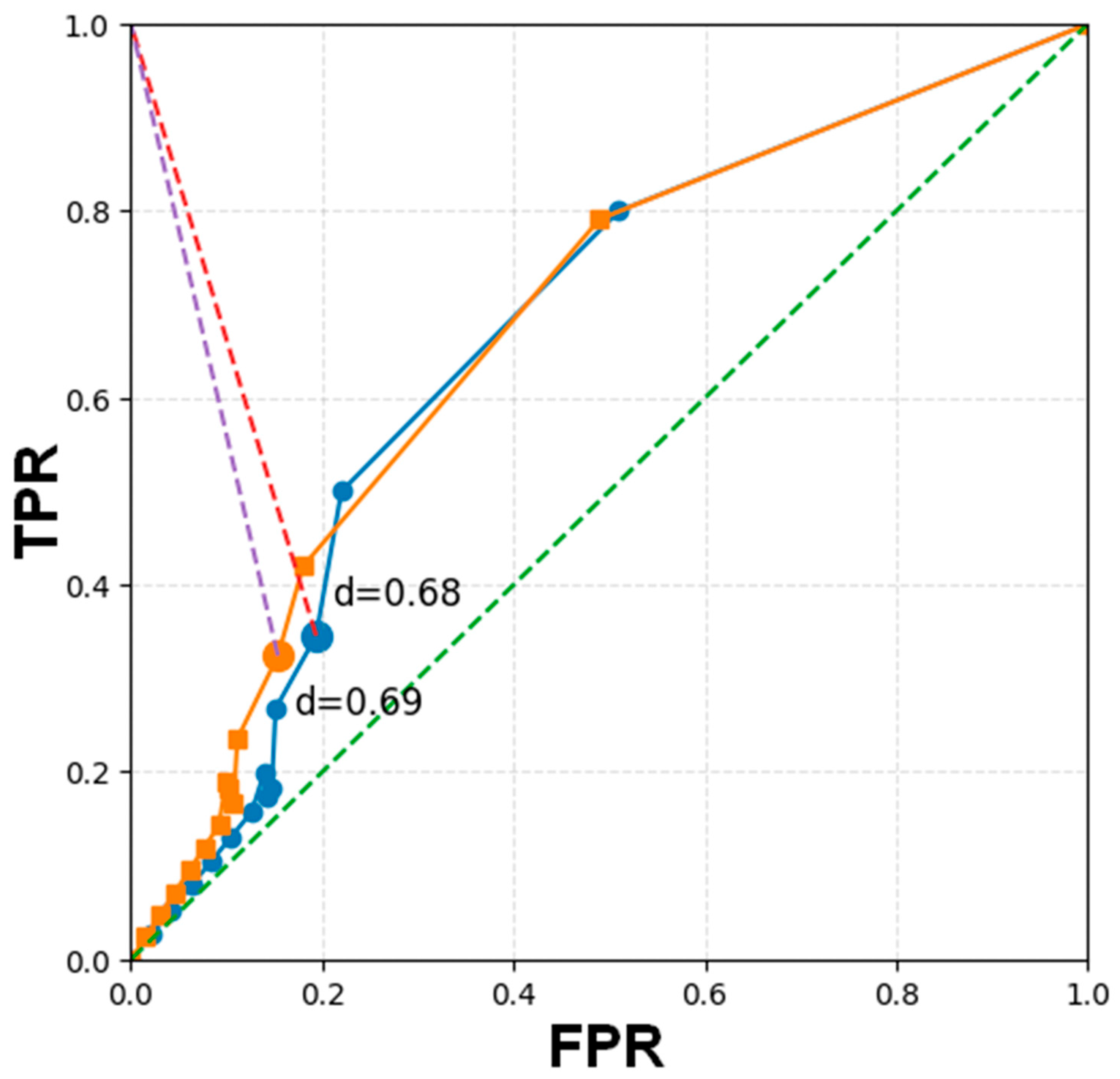
ROC curves are a standard tool in signal detection theory and binary classification in many fields (e.g., [51] in radar, [52] in climate). The ROC curve assesses the ability of S₄ anomalies to distinguish between earthquake-related and non-earthquake ionospheric conditions as shown in Figure 8. TPR shows the proportion of earthquakes correctly preceded by anomalies, while FPR indicates the proportion of anomalies not followed by seismic events. Optimal detection maximizes TPR and minimizes FPR. The threshold coefficient was optimized for each anomaly-detection method using ROC criteria. A chi-square test on the contingency table rejected independence (χ² up to 6.95 × 10⁵, p < 0.001), as shown in

Table 3. ROC performance and statistical metrics across anomaly thresholds.

C	TPR	FPR	ACC	DOR	χ2	OR (95% CI)
0.7	0.34	0.19	0.37	2.20	2.11 × 105	2.20 (2.19–2.20)
1.5	0.20	0.14	0.22	1.53	7.16 × 103	1.53 (1.52–1.55)
2.0	0.17	0.14	0.20	1.27	4.05 × 102	1.27 (1.24–1.30)

. The DOR = 2.20 (95% CI: 2.19–2.20), indicating lower odds in the reference category. Due to the large sample size, the effect size (odds ratio) is emphasized alongside the p-value. Increasing the threshold reduces sensitivity and association strength, showing the trade-off between detection and false alarms. [53]. The minimum distance (d) to the ideal classifier (0,1) is 0.68 for STD and 0.67 for IQR, with IQR being closer to optimal classification [54]. The dashed lines represent the shortest distances, highlighting how close each method is to an ideal classifier. AUC and distance (d) together confirm that IQR has better classification ability. The plot also illustrates the trade-off between TPR and the FPR, a crucial consideration when selecting a classification threshold. The IQR method with C = 0.7 is the optimal configuration for correlation in this analysis, given its higher AUC and lower minimum distance to the optimal classifier.

3.2. CM as a Function of the Earthquake M_w and Depth

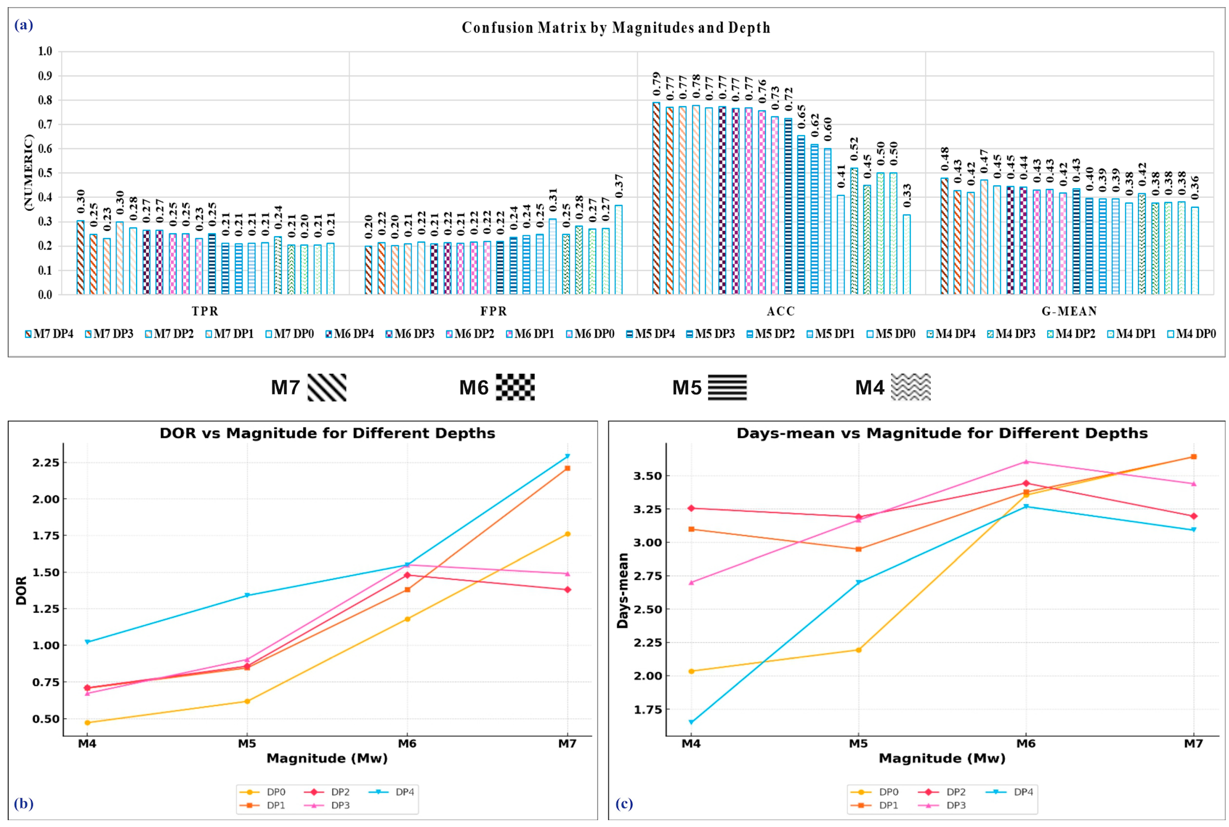
Figure 9 presents the results of a confusion matrix for separated earthquake M_w and depths, illustrating the performance metrics and their physical interpretations. The TPR varies between 0.20 and 0.30, while the ACC ranges from 0.79 to 0.33 at greater depths, indicating significant uncertainty in detecting deep earthquakes. The G-Mean fluctuates between 0.36 and 0.48, underscoring that deeper seismic events are more challenging to predict accurately. From a physical standpoint, the observed trends relate to the nature of seismic wave propagation and energy dissipation. Shallow earthquakes (DP0–DP1) exhibit greater accuracy and predictability because they release energy closer to the surface, resulting in more substantial ground shaking and more detectable signals. In contrast, deep earthquakes (>DP2) occur at greater depths, where high pressure hinders the propagation of fault ruptures, leading to weaker surface impacts and lower detection consistency. The line charts further emphasize this depth-dependent effect. DOR values increase with M_w, exceeding 2.25 for DP4 at M_w ≥ 7, suggesting that deeper earthquakes require more energy to reach detectable thresholds. The Distance-mean peaks at 780 km for DP4 at M_w ≥ 6, then declines at M_w ≥ 7, indicating that deeper seismic events tend to distribute their energy over larger areas but with reduced intensity. Additionally, the Days-mean exceeds 3.5 days for DP3 and DP4 at M_w ≥ 7, indicating that deeper earthquakes are often associated with delayed aftershock sequences and slower energy release due to high-pressure conditions. These results highlight how depth influences earthquake detection, energy release, and response times, making shallow events more predictable but more profound events more difficult to monitor.

3.3. CM as a Function of the Earthquake M_w and Altitude

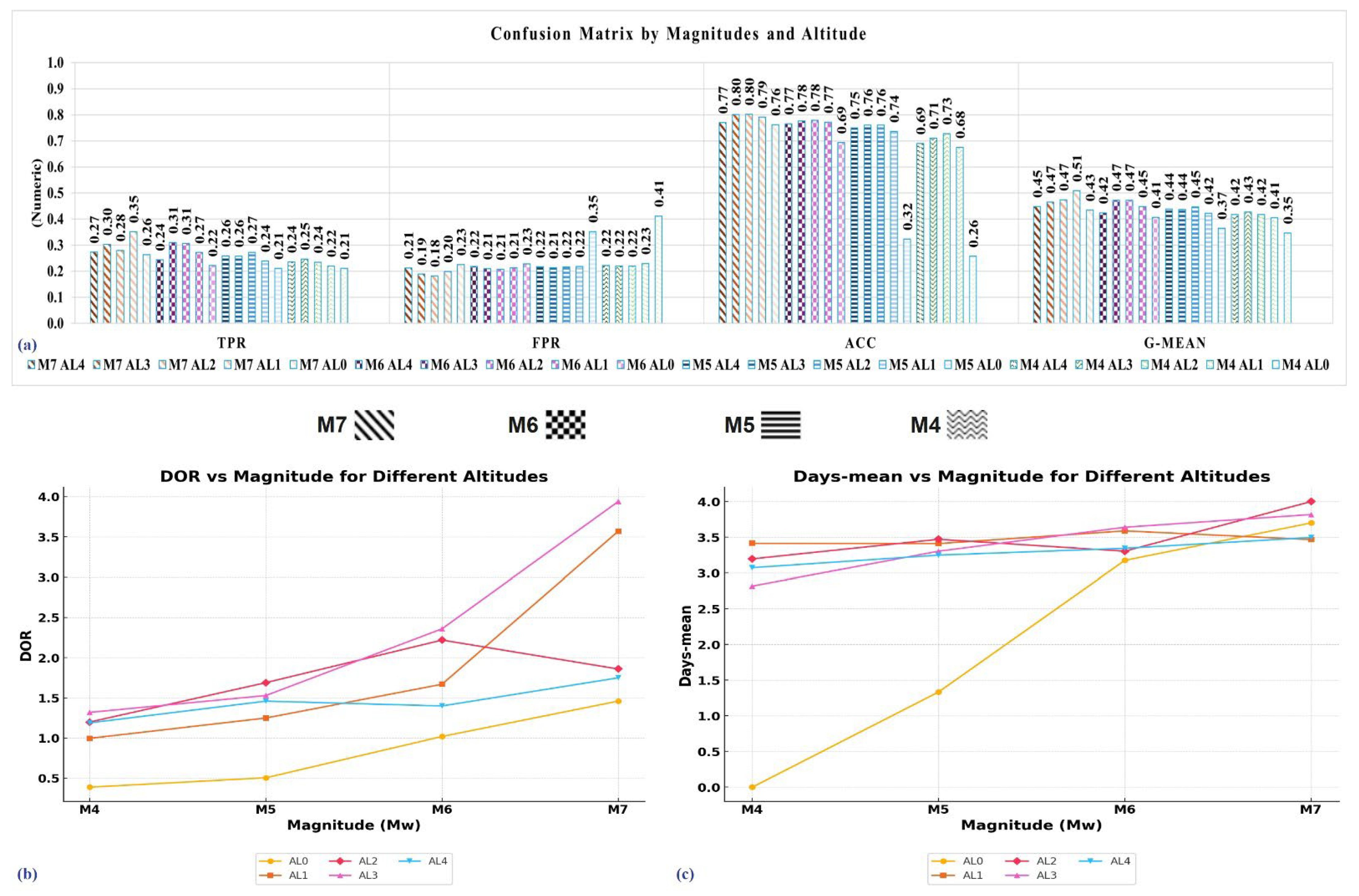
Figure 10 analyzes the confusion matrix by earthquake M_w and altitude, showcasing statistical trends across altitude levels. The TPR ranges from 0.21 to 0.38, while ACC varies considerably from 0.26 to 0.80, suggesting that higher-altitude events are generally well detected. The G-Mean ranges from 0.35 to 0.51, indicating differences in prediction reliability across altitudes. From a physical standpoint, altitude is vital in seismic wave propagation and energy dissipation.

Low-altitude events (AL0–AL1) typically experience weaker surface shaking due to increased ground absorption, resulting in lower detection accuracy and greater variability in response times. In contrast, higher-altitude regions (AL3–AL4) exhibit more substantial surface effects, enhancing detectability but possibly intensifying localized damage. The line charts support this interpretation. DOR values rise with M_w, surpassing 3.5 for AL3 and AL4 at M_w ≥ 7, indicating that high-altitude earthquakes lead to more pronounced surface disturbances. The mean duration exceeds 3.5 days for AL3 and AL4 at M_w ≥ 7, implying that high-altitude events may have extended aftershock sequences and slower energy release. These findings underscore the impact of altitude on earthquake behavior.

3.4. CM as a Function of the Earthquake M_w and Land Cover

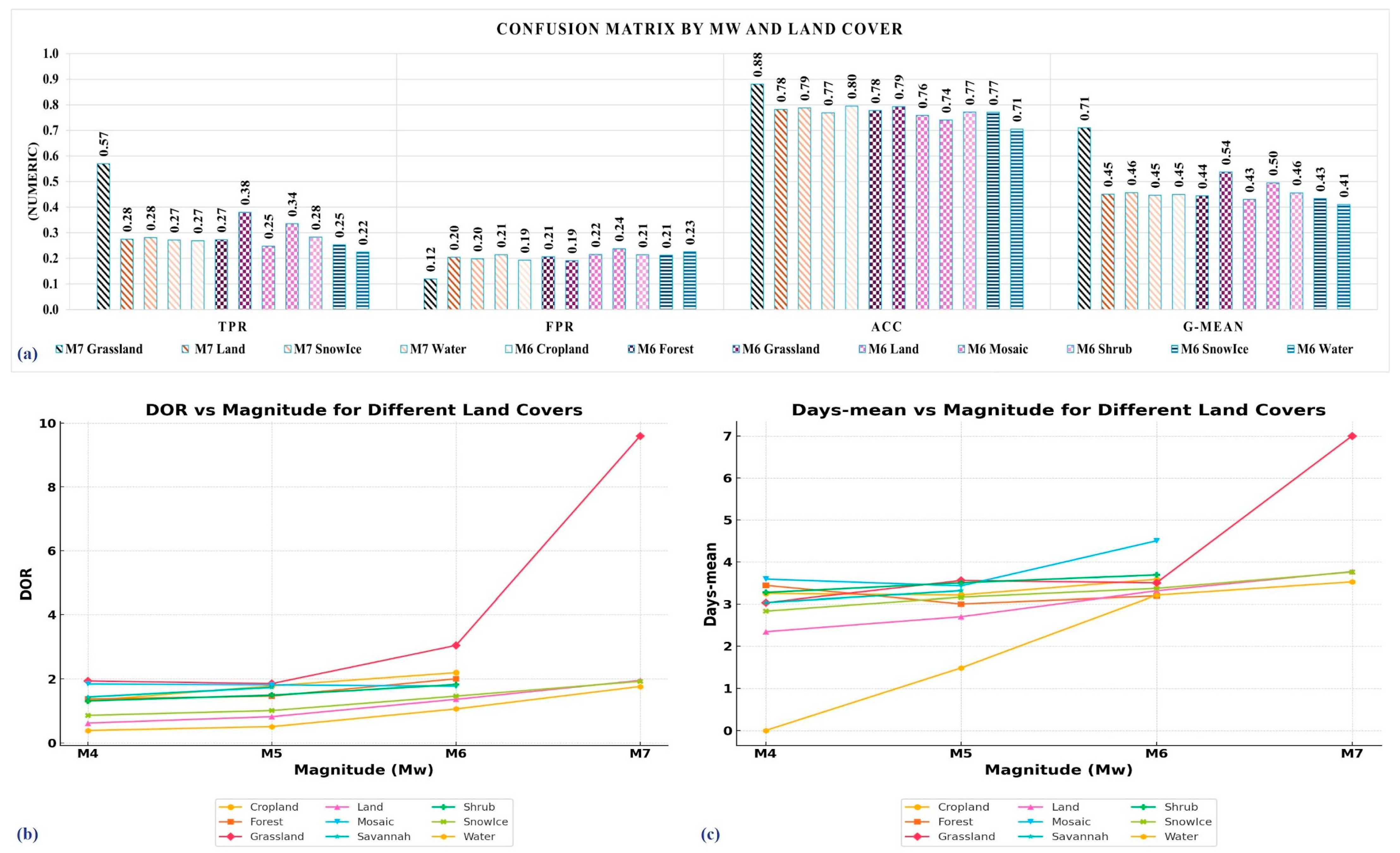
Figure 11 evaluates earthquake M_w and land cover types, detailing detection accuracy and response metrics. The TPR ranges from 0.21 to 0.57, while ACC remains relatively high, reaching 0.88 for specific land covers, particularly grassland. The G-Mean ranges from 0.35 to 0.71, indicating that earthquakes across different land-cover types exhibit varying levels of predictability and impact. From a physical perspective, land cover influences how seismic waves propagate and how ground shaking is transmitted. Forests, croplands, and grasslands absorb seismic energy due to soil and vegetation density, reducing detectability and affecting accuracy. In contrast, hard surfaces like barren land and water bodies allow seismic waves to travel more efficiently, resulting in stronger, more easily detected shaking. The line charts further emphasize these effects. DOR remains relatively stable for most land covers but increases dramatically for barren land at M_w ≥ 7, by almost 10. This suggests that open terrain experiences more substantial and prolonged shaking. The distance varies significantly, peaking above 1000 km for specific land covers at M_w ≥ 7, highlighting differences in wave attenuation across terrains. Additionally, the Days-mean exceeds 7 days for barren lands at M_w ≥ 7, indicating that surface conditions influence seismic energy dissipation and aftershock durations. These findings reinforce the importance of accounting for land cover when modeling earthquake impacts, as different terrain types affect the intensity and duration of seismic activity.

3.5. CM as a Function of the Earthquake M_w and Latitude Region

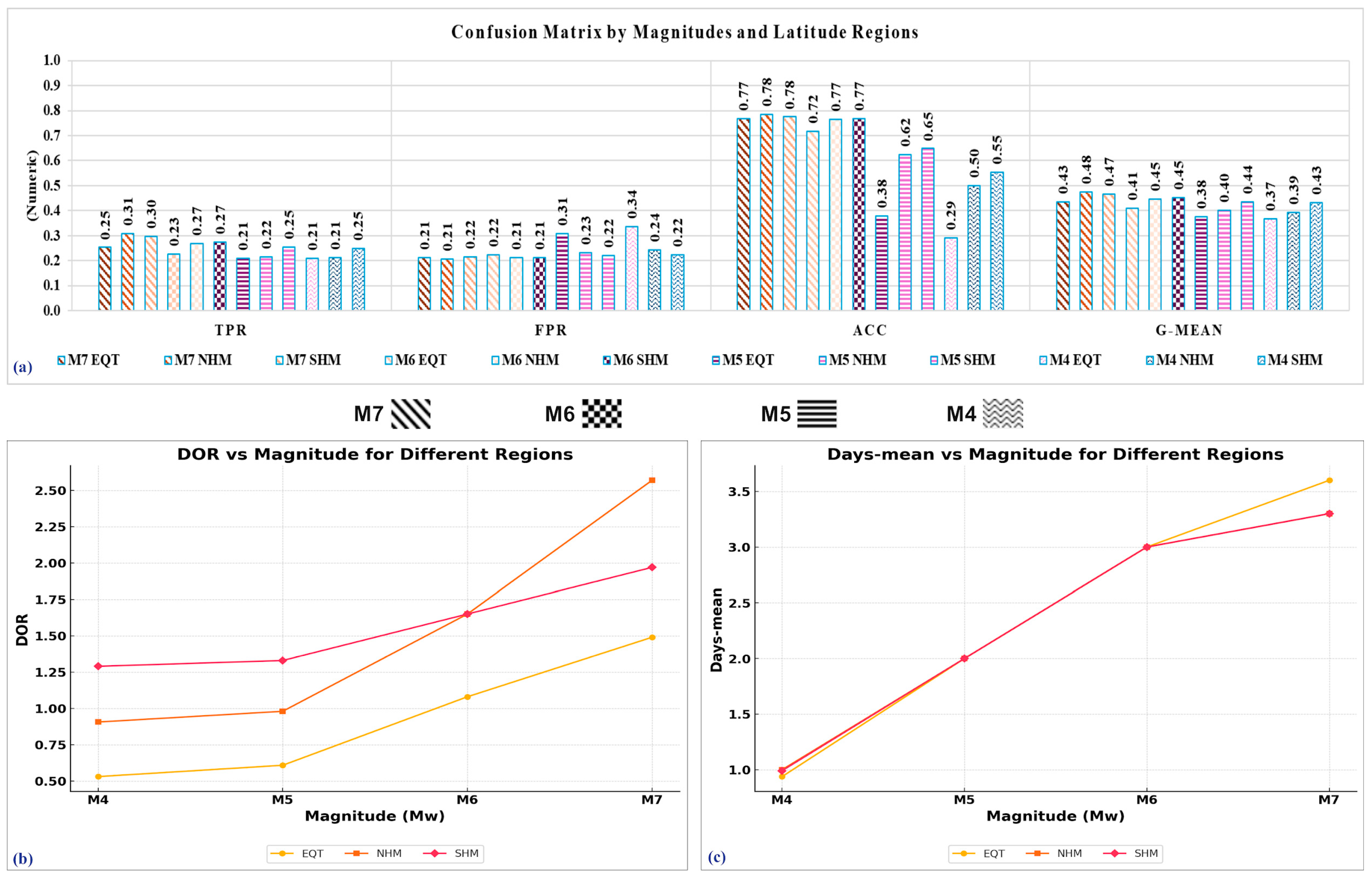
Figure 12 offers statistical and physical insights into earthquake forecasting across different latitudes. Subplot (a) shows TPR between 0.21 and 0.31, indicating moderate detection that improves for stronger earthquakes. FPR ranges from 0.21 to 0.34, signaling false alarms. The ACC (~0.77) and G-Mean (~0.48) peak at M_w ≥ 7 and decrease at lower M_w, indicating that stronger earthquakes produce clearer ionospheric signals. Subplot (b) plots DOR against M_w, revealing DOR increases with M_w, especially in the Southern Hemisphere, likely due to geomagnetic effects. Subplot (c) depicts that larger earthquakes have longer precursor times, consistent with the idea that stronger events release more stress and energy, inducing ionospheric disturbances over longer periods. The Equator and Southern Hemisphere experience slightly longer precursor times, possibly due to stronger electromagnetic interactions in these areas. This figure supports the hypothesis that ionospheric anomalies can be precursors to seismic activity, with stronger earthquakes displaying more precise and longer-lasting signals. The potential influence of longitude on IS anomalies was examined. Unlike latitude, longitude is not systematically related to ionospheric behavior because it is not directly linked to the geomagnetic field. Because the analysis was restricted to nighttime local time (00:00–06:00 LT), longitudinal differences associated with diurnal variation were minimized. Local time is a physically meaningful reference for both ionospheric variability and solar-position effects; for example, Tomiyasu (2007) reported a tendency for many major coastal earthquakes to occur preferentially in morning hours and suggested solar position as a contributing factor [55].

3.6. CM as a Function of the Earthquake M_w and Type

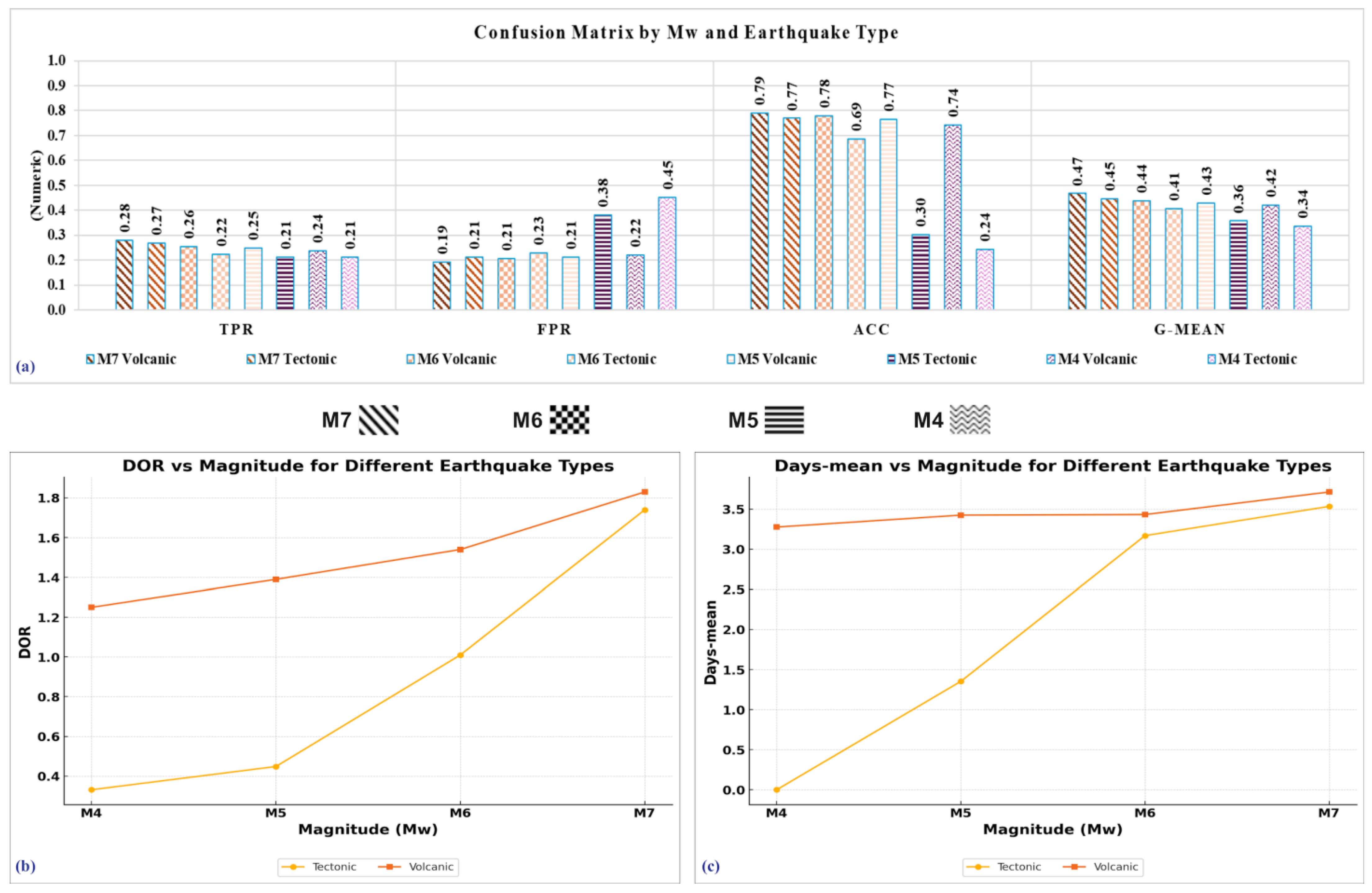
Figure 13 presents statistical analyses of earthquake forecasts based on M_w and earthquake type (tectonic vs. volcanic). From Subplot (a), the TPR ranges from 0.21 to 0.28, indicating that both earthquake types exhibit moderate anomaly-detection rates, with slightly better performance for larger M_w. The FPR is relatively low (0.19–0.45), suggesting few false alarms, but higher values for smaller M_w indicate greater uncertainty in predictions. The ACC (0.79) and G-Mean (0.47) peak at M_w ≥ 7 (~0.77–0.79) and decline for lower M_w, supporting the notion that higher M_w is associated with improved forecast performance. Subplot (b) shows the DOR, which increases with M_w, especially for volcanic earthquakes, suggesting stronger ionospheric coupling driven by volcanic emissions. Subplot (c) shows the average number of days before an earthquake at which anomalies appear, with volcanic earthquakes exhibiting precursor signals earlier than tectonic earthquakes, possibly due to prolonged stress accumulation and outgassing processes that affect the ionosphere. These results suggest that ionospheric anomalies can serve as precursors for both tectonic and volcanic earthquakes, with variations in detection efficiency influenced by earthquake type and M_w. The tectonic setting of the earthquake influences the characteristics of ionospheric scintillation anomalies. Subduction-zone earthquakes, huge ones, tend to produce more extensive and lasting ionospheric disturbances due to their large rupture areas, long durations, and efficient stress buildup at convergent boundaries. Conversely, earthquakes along transform faults usually show more localized ionospheric responses, with narrower rupture zones and shorter source durations.

4. Discussion: Analyzing the Correlation Between S₄ Anomalies and Earthquakes

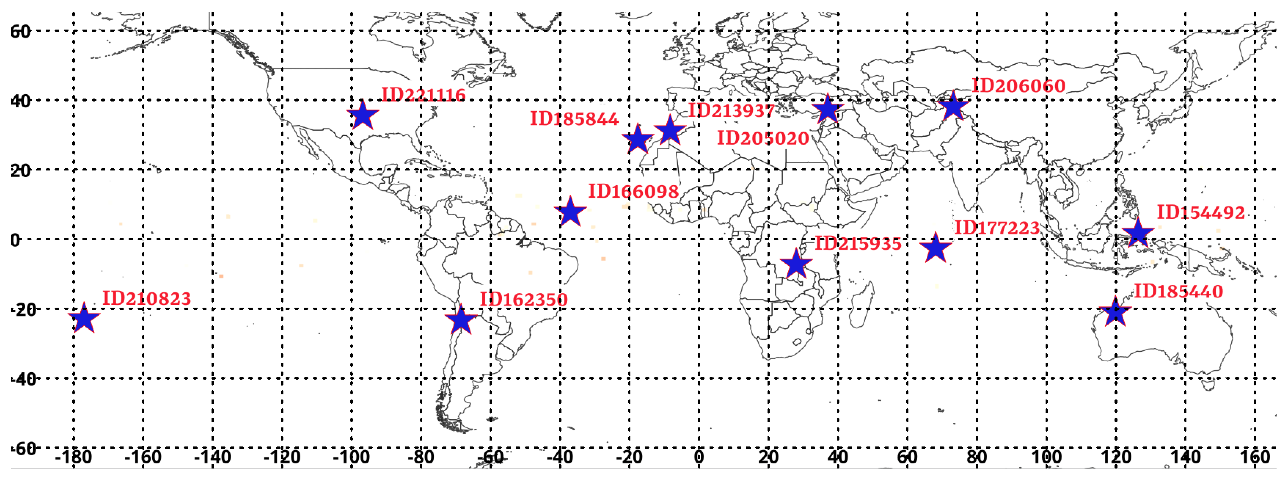
Figure 14 and

Table 4. Details on the illustrated earthquakes as case studies.

ID	Date	Lat (Deg)	Lon (Deg)	Depth (km)	Mag	Strain Radius (km)	Country	Elevation (m)	Region
ID221116	3 February 2024	35.53	−96.76	3	5.1	150	USA	277	NHM
ID215935	26 October 2023	−7.3	27.93	9	5.2	172	Congo	591	EQT
ID213937	8 September 2023	31.06	−8.38	19	6.8	839	Morocco	3149	NHM
ID210823	15 June 2023	−22.99	−177.11	179	7.2	1247	Tonga	0	SHM
ID206060	23 February 2023	38.06	73.23	9	6.9	927	Tajikistan	4912	NHM
ID205020	6 February 2023	37.23	37.01	10	7.8	2259	Turkey	755	NHM
ID185844	23 November 2021	28.7	−17.69	10	4.6	95	La Palma	0	NHM
ID185440	13 November 2021	−20.93	119.81	10	5.3	190	Australia	246	SHM
ID177223	21 May 2021	−2.65	68.1	10	5.8	312	Indian Ocean	0	EQT
ID166098	6 September 2020	7.68	−37.15	10	6.7	760	Brazil	0	EQT
ID162350	3 June 2020	−23.27	−68.47	112	6.8	839	Chile	0	SHM
ID154492	14 November 2019	1.62	126.42	33	7.1	1130	Indonesia	0	EQT

illustrate the 12 case studies. Turkey’s largest earthquake registered at M_w ≥ 7.8. Shallow earthquakes are most common, often causing greater surface damage, whereas the deepest earthquake occurred in Tonga, at a depth of 179 km. Most earthquakes happen around tectonic boundaries, including subduction zones (Tonga, Indonesia, Chile) and transform faults (Turkey). Seismic activity in intraplate regions like Brazil and Australia occurs beyond active plate boundaries. The maximum S₄ value within the studied window was chosen as the anomaly metric because it shows the strongest ionospheric response associated with seismic preparation. This method improves the detection of localized irregularities and aligns with prior scintillation studies that prioritize peak signals over averages.

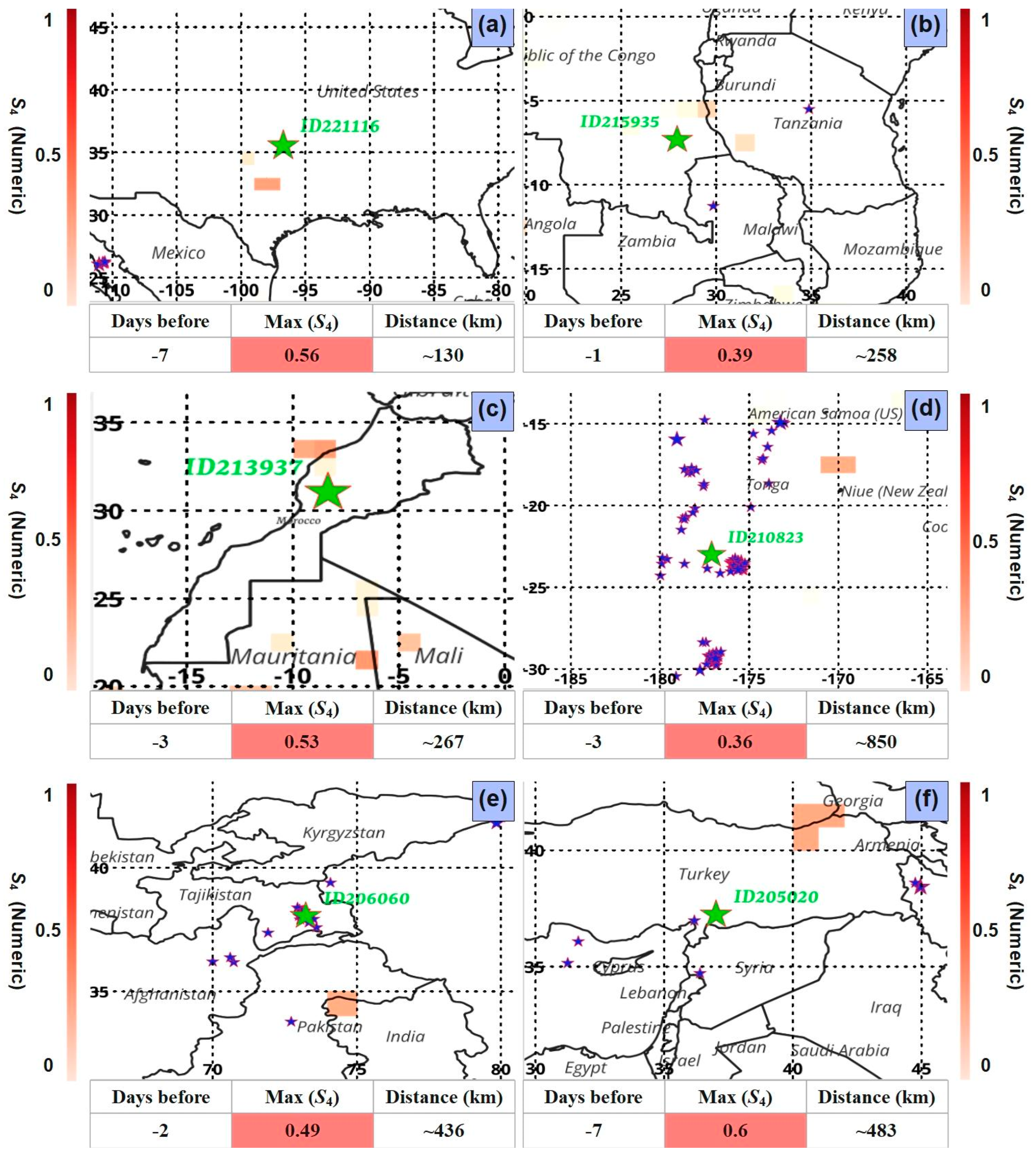
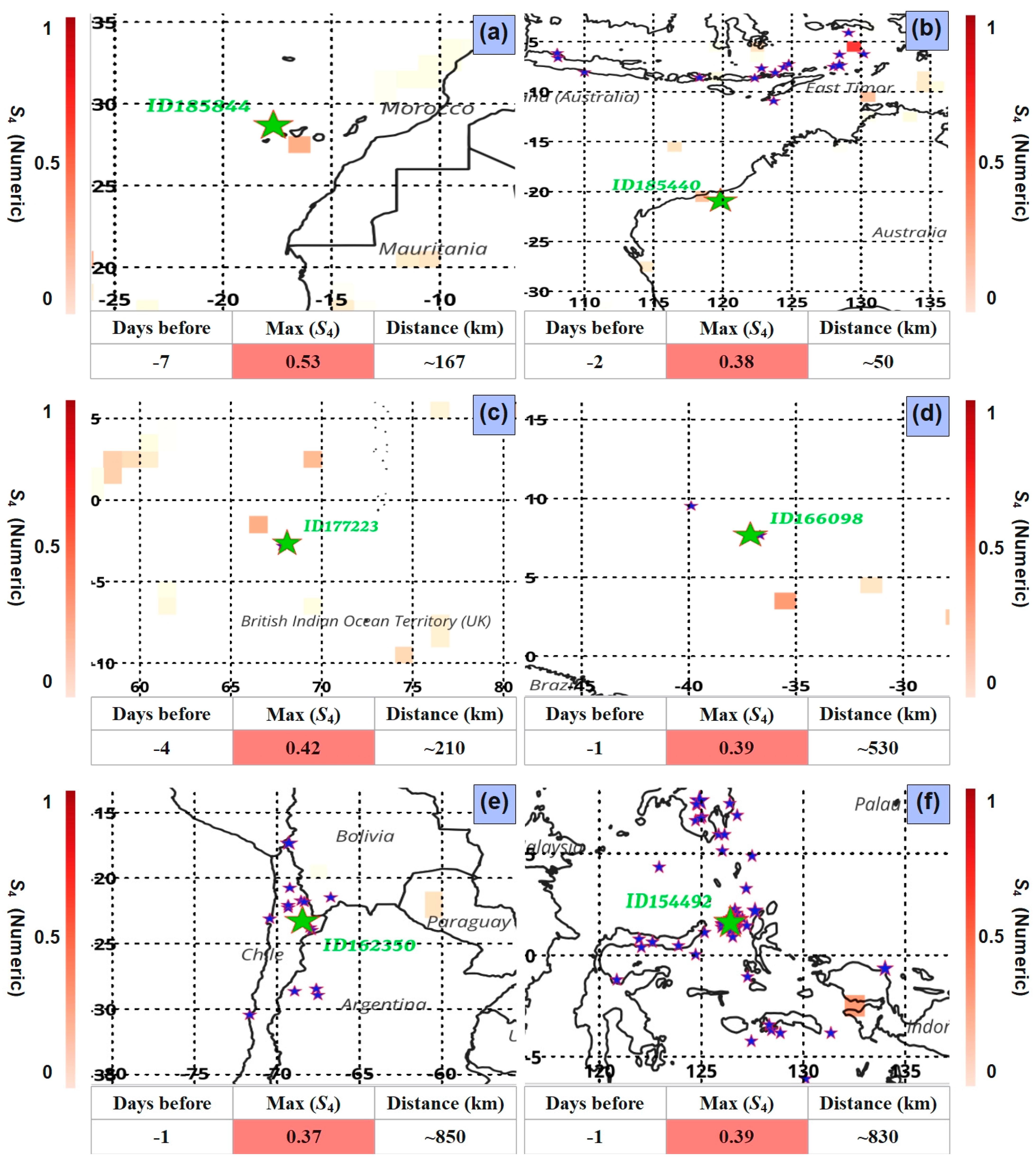
Figure 15 and Figure 16 illustrate the associated S₄ anomalies with a radius of 1000 km and temporal windows of 1 to 7 days before the 12 case studies. The green stars indicate earthquake hypocenters, while the red pixels symbolize the S₄ anomalies. Statistical analysis encompasses three critical parameters: the days leading up to the earthquake when the maximum S₄ value was recorded, the maximum S₄ value, and the approximate distance between the anomaly and the epicenter. For instance, in cases (a) and (f), S₄ peaks of 0.56 and 0.6 were recorded approximately 130 km and 483 km away, respectively, one week before the earthquakes. The variability in these mean distances suggests differences in the geophysical environment across locations.

Case (c), over Morocco, detected an S₄ maximum of 0.53 three days before the earthquake, while case (e), over Pakistan, showed a slightly lower value of 0.49 two days earlier but at a greater distance of 436 km. Meanwhile, case (b), located in Africa, recorded a relatively lower S₄ value of 0.39 just one day before the event at 258 km, demonstrating a more immediate correlation. The Pacific Ocean region (d) observed an anomaly three days beforehand at a much greater distance (~850 km) with an S₄ of 0.36, indicating potential ionospheric or geomagnetic influences extending over a broad area. Case (a) in Morocco shows an S₄ peak of 0.53 recorded seven days prior at 167 km. Case (b), situated near Australia, recorded a lower S₄ value of 0.38 two days before at 50 km, indicating a localized ionospheric disturbance. In the British Indian Ocean Territory (c), an S₄ peak of 0.42 was detected four days before the earthquake, roughly 210 km away. The Atlantic Ocean (d) case shows an S₄ value of 0.39 recorded one day prior at a greater distance of 530 km, suggesting a more extensive ionospheric impact. The South American region (e), encompassing Chile, Argentina, and Bolivia, recorded an S₄ maximum of 0.37 1 day before the earthquake, at 850 km, indicating that anomalies may manifest far from the epicenter. Lastly, the case in the Philippines (f) shows a similar S₄ peak of 0.39 one day prior at 830 km, further supporting the possibility of long-range ionospheric disturbances before seismic events.

The lack of a clear longitudinal dependence contrasts with strong latitude effects, highlighting the influence of geomagnetic geometry and plasma dynamics on ionospheric responses. Earthquake duration is a secondary factor that indirectly affects signatures by influencing rupture size and seismic energy.

The study examined the link between earthquake-related ionospheric anomalies and solar activity, noting that high solar and geomagnetic activity increase turbulence, which can obscure weak signals and reduce detection reliability. Applying geomagnetic and solar filtering improves signal discrimination, but residual space-weather effects may still cause false alarms. Results emphasize the need to consider solar cycle phase and geomagnetic conditions when interpreting ionospheric earthquake precursors.

Solar-activity stratification results from background ionospheric irregularities that increase with solar and geomagnetic activity. We assess solar-cycle dependence by dividing the dataset into activity levels and recalculating detection performance within each group. Detection performance generally declines during high-activity periods due to increased background scintillation, while association metrics remain more consistent under low-to-moderate activity conditions.

Physically, these observations imply that pre-seismic activity influences the Earth’s ionosphere, resulting in measurable electromagnetic perturbations [56]. The S₄ anomalies may arise from stress-induced piezoelectric and electromagnetic emissions [57], gas releases (e.g., radon), or acoustic gravity waves generated by tectonic stress redistribution [36]. The variability in the distances of these anomalies might be related to the propagation of electromagnetic disturbances through the ionosphere or variations in crustal sensitivity across regions [58]. These case studies contribute to the growing evidence supporting ionospheric and electromagnetic monitoring as potential precursors for earthquake forecasting [22]. However, further research is needed to enhance the accuracy and reliability of these methods [59].

Despite significant correlations, ionospheric signals are weak and probabilistic, hindering deterministic earthquake prediction. Space-weather contamination, localization uncertainty, and background variability all contribute to uncertainty. Relying on one parameter (S₄) limits interpretation, underscoring the need for multiparametric approaches. Detectability is also affected by solar cycle variability and geomagnetic storms.

5. Conclusions

This study investigates S₄ anomalies associated with over 71,000 earthquakes between 2019 and 2024, using time-series data from the COSMIC-2 GNSS-RO. Twelve earthquakes have been selected as case studies to illustrate the findings. The observed variations in S₄ activities indicate that IS is linked to equatorial plasma depletion. This work demonstrates that S₄ anomalies can also serve as proxies for seismic activity.

A geospatial earthquake mask and the SAF filter were used to ensure data quality and to reduce false alarms caused by intense solar radiation. S₄ anomalies were assessed using the STD and IQR methods, applying multiple threshold coefficients (0.5, 0.7, 1, 1.5, 2, and 2.5). A confusion matrix and ROC curves were generated for each threshold to determine the best configuration and threshold. These analyses were conducted separately for earthquakes categorized by M_w, depth, latitude, land cover, and type.

The results show a clear positive correlation between earthquakes with M_w ≥ 4, with stronger correlations observed as M_w increases. The optimal threshold for earthquake forecasting was identified at C = 0.7. Under the optimal threshold (C = 0.7), the probability of correct prediction was approximately 35%, while the false-alarm probability remained limited to roughly 19%. The optimal detection point corresponds to a Euclidean distance of d ≈ 0.68, yielding an AUC of approximately 0.67–0.68 and a DOR of about 2.2, indicating a statistically significant but moderate discriminative performance. Despite these results, the detected signal remains weak and inconsistent for an early earthquake warning system. The results show probabilistic correlations rather than deterministic earthquake prediction and should be considered within a statistical seismo-ionospheric framework.

Therefore, future research should investigate the potential integration of additional geophysical parameters, such as LST anomalies, magnetic field disturbances from Swarm, and IS derived from GNSS-R measurements, to understand their connection to earthquake activity better. A future multi-parameter warning model may integrate normalized anomaly indices from S₄, TEC, magnetic-field residuals, and Faraday rotation. Spatio-temporal co-registration can be performed using adaptive spatial buffers (scaled to the M_w-dependent strain radius) and time-lagged association measures (cross-correlation/mutual information) within parameter-specific precursor windows. Model fusion can be implemented via dynamic weighting or a probabilistic graphical model that accounts for differing latency and spatial footprints.

References

1. Wu, D.L. Ionospheric S4 Scintillations from GNSS Radio Occultation (RO) at Slant Path. Remote Sens. 2020, 12, 2373. [Google Scholar] [CrossRef]
2. Li, W.; Zhao, D.; Feng, J.; Wu, X.; Zhang, Z. Spatial Development of Strong Storm-Induced Ionospheric Perturbations during 25–27 August 2018. Remote Sens. 2023, 15, 2549. [Google Scholar] [CrossRef]
3. Liu, J.-Y.; Lin, C.-H.; Rajesh, P.K.; Lin, C.-Y.; Chang, F.-Y.; Lee, I.-T.; Fang, T.-W.; Fuller-Rowell, D.; Chen, S.-P. Advances in Ionospheric Space Weather by Using FORMOSAT-7/COSMIC-2 GNSS Radio Occultations. Atmosphere 2022, 13, 858. [Google Scholar] [CrossRef]
4. Zhang, F.-Z.; Huang, J.-P.; Li, Z.; Shen, X.-H.; Li, W.-J.; Wang, Q.; Zeren, Z.; Liu, J.-L.; Li, Z.-Y.; Chen, Z.-Y. Statistical Analysis of Electric Field Perturbations in ELF Based on the CSES Observation Data before the Earthquake. Front. Earth Sci. 2023, 11, 1101542. [Google Scholar] [CrossRef]
5. Prasanna Simha, C.; Natarajan, V.; Rao, K.M. Pre-Earthquake Atmospheric and Ionospheric Anomalies before Taiwan Earthquakes (M 6.1 and M 6.4) on February (4th and 6th), 2018. Geomagn. Aeron. 2020, 60, 644–660. [Google Scholar] [CrossRef]
6. Boudriki Semlali, B.-E.; Molina, C.; Librado, M.C.; Park, H.; Camps, A. Potential Earthquake Proxies from Remote Sensing Data; IntechOpen: London, UK, 2024. [Google Scholar] [CrossRef]
7. Mignan, A.; Ouillon, G.; Sornette, D.; Freund, F. Global Earthquake Forecasting System (GEFS): The Challenges Ahead. Eur. Phys. J. Spec. Top. 2021, 230, 473–490. [Google Scholar] [CrossRef]
8. Boudriki Semlali, B.-E.; Molina, C.; Park, H.; Camps, A. On the Correlation Between Earthquakes and Prior Ionospheric Scintillations Over the Ocean: A Study Using GNSS-R Data Between 2017 and 2021. IEEE J. Sel. Top. Appl. Earth Obs. Remote Sens. 2024, 17, 2640–2654. [Google Scholar] [CrossRef]
9. De Santis, A.; Perrone, L.; Calcara, M.; Campuzano, S.A.; Cianchini, G.; D’Arcangelo, S.; Di Mauro, D.; Marchetti, D.; Nardi, A.; Orlando, M.; et al. A Comprehensive Multiparametric and Multilayer Approach to Study the Preparation Phase of Large Earthquakes from Ground to Space: The Case Study of the June 15 2019, M7.2 Kermadec Islands (New Zealand) Earthquake. Remote Sens. Environ. 2022, 283, 113325. [Google Scholar] [CrossRef]
10. Molina, C.; Boudriki Semlali, B.-E.; Park, H.; Camps, A. A Preliminary Study on Ionospheric Scintillation Anomalies Detected Using GNSS-R Data from NASA CYGNSS Mission as Possible Earthquake Precursors. Remote Sens. 2022, 14, 2555. [Google Scholar] [CrossRef]
11. Molina, C.; Boudriki Semlali, B.-E.; González-Casado, G.; Park, H.; Camps, A. The 2021 La Palma Volcanic Eruption and Its Impact on Ionospheric Scintillation as Measured from GNSS Reference Stations, GNSS-R and GNSS-RO. Nat. Hazards Earth Syst. Sci. 2023, 23, 3671–3684. [Google Scholar] [CrossRef]
12. Carvajal-Librado, M.; Molina, C.; Boudriki-Semali, B.E.; Park, H.; Camps, A. Analyzing GNSS-RO Derived Ionospheric Intensity Scintillation Preceding Earthquakes in the Coral Sea During 2022. IEEE J. Sel. Top. Appl. Earth Obs. Remote Sens. 2024, 17, 16020–16029. [Google Scholar] [CrossRef]
13. Iwata, T.; Umeno, K. Preseismic Ionospheric Anomalies Detected before the 2016 Kumamoto Earthquake. JGR Space Phys. 2017, 122, 3602–3616. [Google Scholar] [CrossRef]
14. Wen, Y.; Wang, G.; Tao, D.; Zong, J.; Zeren, Z.; Shen, X. Seismic-Ionospheric Perturbations in Ionospheric TEC and Plasma Parameters Associated with the 14 July 2019 & nbsp; Mw7.2 Laiwui Earthquake Detected by the GPS and CSES. arXiv 2021, arXiv:2102.03536. [Google Scholar]
15. Li, Z.; Li, J.; Huang, J.; Yin, H.; Jia, J. Research on Pre-Seismic Feature Recognition of Spatial Electric Field Data Recorded by CSES. Atmosphere 2022, 13, 179. [Google Scholar] [CrossRef]
16. Chou, M.; Yue, J.; Wang, J.; Huba, J.D.; El Alaoui, M.; Kuznetsova, M.M.; Rastätter, L.; Shim, J.S.; Fang, T.; Meng, X.; et al. Validation of Ionospheric Modeled TEC in the Equatorial Ionosphere During the 2013 March and 2021 November Geomagnetic Storms. Space Weather 2023, 21, e2023SW003480. [Google Scholar] [CrossRef]
17. Boudriki Semlali, B.-E.; Molina, C.; Park, H.; Camps, A. Global Correlation of Swarm Satellites Magnetic Field and TEC Data with M4+ Earthquakes between 2014 and 2024. Adv. Space Res. 2025, 75, 7589–7609. [Google Scholar] [CrossRef]
18. Idosa Uga, C.; Prasad Gautam, S.; Beshir Seba, E. Impact of Geomagnetic Storms on Ionospheric TEC at High Latitude Stations: A Comparative Analysis of GPS Observations and the IRI-2016 Model. Astrophys. Space Sci. 2023, 368, 85. [Google Scholar] [CrossRef]
19. Savastano, G.; Nordström, K.; Angling, M.J. Semi-Supervised Classification of Lower-Ionospheric Perturbations Using GNSS Radio Occultation Observations from Spire Global’s Cubesat Constellation. J. Space Weather Space Clim. 2022, 12, 14. [Google Scholar] [CrossRef]
20. Pulinets, S.; Ouzounov, D. Lithosphere–Atmosphere–Ionosphere Coupling (LAIC) Model—An Unified Concept for Earthquake Precursors Validation. J. Asian Earth Sci. 2011, 41, 371–382. [Google Scholar] [CrossRef]
21. Akhoondzadeh, M.; De Santis, A.; Marchetti, D.; Shen, X. Swarm-TEC Satellite Measurements as a Potential Earthquake Precursor Together With Other Swarm and CSES Data: The Case of Mw7.6 2019 Papua New Guinea Seismic Event. Front. Earth Sci. 2022, 10, 820189. [Google Scholar] [CrossRef]
22. De Santis, A.; Balasis, G.; Pavón-Carrasco, F.J.; Cianchini, G.; Mandea, M. Potential Earthquake Precursory Pattern from Space: The 2015 Nepal Event as Seen by Magnetic Swarm Satellites. Earth Planet. Sci. Lett. 2017, 461, 119–126. [Google Scholar] [CrossRef]
23. Boudriki Semlali, B.-E.; Molina, C.; Park, H.; Camps, A. First Results on the Systematic Search of Land Surface Temperature Anomalies as Earthquakes Precursors. Remote Sens. 2023, 15, 1110. [Google Scholar] [CrossRef]
24. Boudriki Semlali, B.-E.B.; Molina, C.; Park, H.; Camps, A. All-Sky LST Anomaly Detection Associated to the Türkiye February 6th, 2023, Mw = 7.8, and Morocco September 9th, 2023, Mw = 6.8 Earthquakes. In Recent Research on Sedimentology, Stratigraphy, Paleontology, Tectonics, Geochemistry, Volcanology and Petroleum Geology; Advances in Science, Technology & Innovation; Çiner, A., Banerjee, S., Radwan, A., Hamimi, Z., Candeias, C., Meghraoui, M., Laouar, R., Eds.; Springer Nature: Cham, Switzerland, 2025; pp. 461–465. ISBN 978-3-031-87557-1. [Google Scholar]
25. Ghosh, S.; Chowdhury, S.; Kundu, S.; Sasmal, S.; Politis, D.Z.; Potirakis, S.M.; Hayakawa, M.; Chakraborty, S.; Chakrabarti, S.K. Unusual Surface Latent Heat Flux Variations and Their Critical Dynamics Revealed before Strong Earthquakes. Entropy 2021, 24, 23. [Google Scholar] [CrossRef] [PubMed]
26. Chakraborty, S.; Sasmal, S.; Chakrabarti, S.K.; Bhattacharya, A. Observational Signatures of Unusual Outgoing Longwave Radiation (OLR) and Atmospheric Gravity Waves (AGW) as Precursory Effects of May 2015 Nepal Earthquakes. J. Geodyn. 2018, 113, 43–51. [Google Scholar] [CrossRef]
27. Yusof, K.A.; Abdullah, M.; Hamid, N.S.A.; Ahadi, S.; Ghamry, E. Statistical Global Investigation of Pre-Earthquake Anomalous Geomagnetic Diurnal Variation Using Superposed Epoch Analysis. IEEE Trans. Geosci. Remote Sens. 2022, 60, 2001413. [Google Scholar] [CrossRef]
28. Smirnov, S. Earth Electric Field Negative Anomalies as Earthquake Precursors. E3S Web Conf. 2020, 196, 01004. [Google Scholar] [CrossRef]
29. Gazquez, J.A.; Garcia, R.M.; Castellano, N.N.; Fernandez-Ros, M.; Perea-Moreno, A.-J.; Manzano-Agugliaro, F. Applied Engineering Using Schumann Resonance for Earthquakes Monitoring. Appl. Sci. 2017, 7, 1113. [Google Scholar] [CrossRef]
30. Hayakawa, M.; Nickolaenko, A.P.; Galuk, Y.P.; Kudintseva, I.G. Manifestations of Nearby Moderate Earthquakes in Schumann Resonance Spectra. IJEAR 2020, 7, 1–28. [Google Scholar] [CrossRef]
31. Haider, S.F.; Shah, M.; Li, B.; Jamjareegulgarn, P.; De Oliveira-Júnior, J.F.; Zhou, C. Synchronized and Co-Located Ionospheric and Atmospheric Anomalies Associated with the 2023 Mw 7.8 Turkey Earthquake. Remote Sens. 2024, 16, 222. [Google Scholar] [CrossRef]
32. Boudriki Semlali, B.-E.; El Amrani, C.; Ortiz, G. SAT-ETL-Integrator: An Extract-Transform-Load Software for Satellite Big Data Ingestion. J. Appl. Remote Sens. (JARS) 2020, 14, 28. [Google Scholar] [CrossRef]
33. Boudriki Semlali, B.-E.; Freitag, F. SAT-Hadoop-Processor: A Distributed Remote Sensing Big Data Processing Software for Earth Observation Applications. Appl. Sci. 2021, 11, 10610. [Google Scholar] [CrossRef]
34. CALCULA Computing Services. Available online: https://tsc.upc.edu/en/it-services/computing-services (accessed on 14 March 2025).
35. Molina, C.; Boudriki Semlali, B.-E.; González-Casado, G.; Park, H.; Camps, A. Ionospheric Scintillation Anomalies Associated with the 2021 La Palma Volcanic Eruption Detected with Gnss-R and Gnss-Ro Observations. In Proceedings of the IGARSS 2022–2022 IEEE International Geoscience and Remote Sensing Symposium, Kuala Lumpur, Malaysia, 17–22 July 2022; pp. 7445–7448. [Google Scholar]
36. Iyemori, T.; Nose, M.; Han, D.; Gao, Y.; Hashizume, M.; Choosakul, N.; Shinagawa, H.; Tanaka, Y.; Utsugi, M.; Saito, A.; et al. Geomagnetic Pulsations Caused by the Sumatra Earthquake on December 26, 2004. Geophys. Res. Lett. 2005, 32, 2005GL024083. [Google Scholar] [CrossRef]
37. Librado, M.C.; Molina, C.; Semlali, B.E.B.; Park, H.; Camps, A. Correlation Between Ionosphere Scintillation and Earthquakes Around Coral Sea in 2022. In Proceedings of the IGARSS 2023–2023 IEEE International Geoscience and Remote Sensing Symposium; IEEE: Pasadena, CA, USA, 2023; pp. 2346–2349. [Google Scholar]
38. Boudriki Semlali, B.-E.; El Amrani, C.; Ortiz, G. Adopting the Hadoop Architecture to Process Satellite Pollution Big Data. Int. J. Technol. Eng. Stud. 2019, 5, 30–39. [Google Scholar] [CrossRef]
39. Boudriki Semlali, B.-E.; Molina, C.; Park, H.; Camps, A. Study of Land Surface Temperature Anomalies Associated to Earthquakes Using GOES Data. In Proceedings of the IGARSS 2022–2022 IEEE International Geoscience and Remote Sensing Symposium, Kuala Lumpur, Malaysia, 17–22 July 2022; pp. 5732–5735. [Google Scholar]
40. Molina, C.; Boudriki Semlali, B.-E.; Park, H.; Camps, A. Possible Evidence of Earthquake Precursors Observed in Ionospheric Scintillation Events Observed from Spaceborne GNSS-R Data. In Proceedings of the 2021 IEEE International Geoscience and Remote Sensing Symposium IGARSS, Brussels, Belgium, 12–16 July 2021; pp. 8680–8683. [Google Scholar]
41. Anthes, R.A. Exploring Earth’s Atmosphere with Radio Occultation: Contributions to Weather, Climate and Space Weather. Atmos. Meas. Tech. 2011, 4, 1077–1103. [Google Scholar] [CrossRef]
42. CDAAC: COSMIC Data Analysis and Archive Center–CDAAC Description. Available online: https://cdaac-www.cosmic.ucar.edu/cdaac/cgi_bin/fileFormats.cgi?type=podTc2 (accessed on 14 March 2025).
43. Schreiner, W.S.; Weiss, J.P.; Anthes, R.A.; Braun, J.; Chu, V.; Fong, J.; Hunt, D.; Kuo, Y.-H.; Meehan, T.; Serafino, W.; et al. COSMIC-2 Radio Occultation Constellation: First Results. Geophys. Res. Lett. 2020, 47, e2019GL086841. [Google Scholar] [CrossRef]
44. Yu, X.; Yue, X.; Zhen, W.; Xu, J.; Liu, D.; Guo, S. On the Occurrence of F Region Irregularities over Haikou Retrieved from COSMIC GPS Radio Occultation and Ground-Based Ionospheric Scintillation Monitor Observations: Occurrence of F Region Irregularities. Radio Sci. 2017, 52, 34–48. [Google Scholar] [CrossRef]
45. Jordan, A. GFZ Data Center. Available online: https://www.gfz-potsdam.de/en/section/geomagnetism/data-products-services/geomagnetic-kp-index (accessed on 29 May 2023).
46. Chappell, C.R.; Schunk, R.W.; Banks, P.M.; Burch, J.L.; Thorne, R.M. (Eds.) Magnetosphere-Ionosphere Coupling in the Solar System; Geophysical monograph; Wiley: Hoboken, NJ, USA, 2017; ISBN 978-1-119-06677-4. [Google Scholar]
47. Wang, Y.; Yuan, Y.; Li, M.; Zhang, T.; Geng, H.; Wang, G.; Wen, G. Effects of Strong Geomagnetic Storms on the Ionosphere and Degradation of Precise Point Positioning Accuracy during the 25th Solar Cycle Rising Phase: A Case Study. Remote Sens. 2023, 15, 5512. [Google Scholar] [CrossRef]
48. ANSS—Advanced National Seismic System|U.S. Geological Survey. Available online: https://www.usgs.gov/programs/earthquake-hazards/anss-advanced-national-seismic-system (accessed on 14 March 2025).
49. National Earthquake Information Center (NEIC)|U.S. Geological Survey. Available online: https://www.usgs.gov/programs/earthquake-hazards/national-earthquake-information-center-neic (accessed on 14 March 2025).
50. ShakeMap. Available online: https://earthquake.usgs.gov/data/shakemap/ (accessed on 14 March 2025).
51. Richards, M.A. Fundamentals of Radar Signal Processing, 3rd ed.; McGraw Hill LLC: New York, NY, USA, 2022; ISBN 978-1-260-46871-7. [Google Scholar]
52. Kharin, V.V.; Zwiers, F.W. On the ROC Score of Probability Forecasts. J. Clim. 2003, 16, 4145–4150. [Google Scholar] [CrossRef]
53. Fawcett, T. An Introduction to ROC Analysis. Pattern Recognit. Lett. 2006, 27, 861–874. [Google Scholar] [CrossRef]
54. Bradley, A.P. The Use of the Area under the ROC Curve in the Evaluation of Machine Learning Algorithms. Pattern Recognit. 1997, 30, 1145–1159. [Google Scholar] [CrossRef]
55. Tomiyasu, K. Local Times of Major Earthquakes in Coastal Regions. In Proceedings of the 2007 IEEE International Geoscience and Remote Sensing Symposium, Barcelona, Spain, 23–28 July 2007; pp. 2987–2988. [Google Scholar]
56. Hayakawa, M.; Schekotov, A.; Izutsu, J.; Nickolaenko, A.P. Seismogenic Effects in ULF/ELF/VLF Electromagnetic Waves. IJEAR 2019, 6, 1–86. [Google Scholar] [CrossRef]
57. Freund, F.T. Pre-Earthquake Signals—Part I: Deviatoric Stresses Turn Rocks into a Source of Electric Currents. Nat. Hazards Earth Syst. Sci. 2007, 7, 535–541. [Google Scholar] [CrossRef]
58. Harrison, R.G.; Aplin, K.L.; Rycroft, M.J. Atmospheric Electricity Coupling between Earthquake Regions and the Ionosphere. J. Atmos. Sol. Terr. Phys. 2010, 72, 376–381. [Google Scholar] [CrossRef]
59. Liu, J.Y.; Chen, C.H.; Tsai, H.F. A Statistical Study on Seismo-Ionospheric Precursors of the Total Electron Content Associated with 146 M ≥ 6.0 Earthquakes in Japan during 1998–2011. In Earthquake Prediction Studies: Seismo Electromagnetics; TERRAPUB: Tokyo, Japan, 2013. [Google Scholar]
Figure 1. Overall processing architecture for COSMIC-2 S4 data ingestion and analysis. The workflow includes data extraction, filtering, statistical anomaly detection, and correlation analysis. Color-coded blocks represent the main processing stages.
Ijgi 15 00128 g001
Figure 2. Schematic representation of the GNSS-RO geometry used for ionospheric sensing. The GNSS signal propagates through the ionosphere and is received by a Low-Earth-Orbit satellite. The tangent point indicates the location where the S4 scintillation index is estimated [11].
Ijgi 15 00128 g002
Figure 3. Map of the filtered dataset by the earthquake frequency mask during 2019 and 2024.
Ijgi 15 00128 g003
Figure 4. Seasonal aggregation maps of IS parameters for Spring 2022. From top to bottom: STD, IQR, and mean S4 values. All metrics are computed on a 1° × 1° geographic grid.
Ijgi 15 00128 g004
Figure 5. Example of spatiotemporal association between S4 anomalies and earthquake occurrences on 18 January 2023. Red pixels indicate detected S4 anomalies, while green stars represent earthquake epicenters. TP, FP, and FN are highlighted based on the predefined spatial (≤1000 km) and temporal (1–7 days) correlation windows used in the confusion matrix analysis.
Ijgi 15 00128 g005
Figure 6. Global distribution of earthquakes with Mw ≥ 4 recorded between 2019 and 2024. Earthquake epicenters are color-coded according to magnitude. The spatial pattern highlights major tectonic plate boundaries and seismic belts.
Ijgi 15 00128 g006
Figure 7. Statistical description of the earthquake dataset used in this study. Distributions are shown for depth, altitude, land-cover type, and earthquake classification. These statistics provide context for the correlation analyses.
Ijgi 15 00128 g007
Figure 8. ROC curves for S4 anomaly detection using STD and IQR methods. ROC curves are shown for all tested threshold coefficients (C = 0.5–2.5).
Ijgi 15 00128 g008
Figure 9. (a) Confusion matrix performance metrics as a function of earthquake magnitude and depth (b) DOR performance as a function of earthquake magnitude and depth, and (c) the number of days before. Results show reduced detectability for deeper seismic events.
Ijgi 15 00128 g009
Figure 10. (a) Confusion matrix performance metrics as a function of earthquake magnitude and altitudes; (b) DOR as a function of magnitude and altitudes; (c) variation of the detection performance with the number of days before the earthquake. As a result, higher-altitude regions generally exhibit stronger ionospheric responses.
Ijgi 15 00128 g010
Figure 11. (a) Confusion matrix performance metrics according to earthquake magnitude and land covers; (b) DOR as a function of magnitude and land covers; (c) detection performance relative to the number of days preceding the earthquake. Different surface conditions influence seismic wave propagation and ionospheric coupling. Accordingly, Barren and water-covered regions show higher anomaly detectability.
Ijgi 15 00128 g011
Figure 12. (a) Confusion-matrix–based performance across earthquake magnitude and latitude regions; (b) DOR Vs magnitude and latitude regions; (c) detection performance as a function of days before the event. Larger earthquakes tend to exhibit stronger and earlier ionospheric signatures.
Ijgi 15 00128 g012
Figure 13. (a) Confusion-matrix–based performance across earthquake magnitude and earthquake type; (b) DOR across magnitude and earthquake type; (c) detection performance as a function of days before the event. Volcanic events tend to exhibit slightly earlier precursor signals.
Ijgi 15 00128 g013
Figure 14. Geographical locations of the 12 selected earthquake case studies. The case studies span different tectonic environments, including subduction zones, transform faults, and intraplate regions, providing representative examples for detailed analysis of the S4 anomaly.
Ijgi 15 00128 g014
Figure 15. Spatial distribution of S4 anomalies associated with selected earthquake case studies (part 1). Anomalies are shown within a 1000 km radius and 1–7 days before each event.
Ijgi 15 00128 g015
Figure 16. Spatial distribution of S4 anomalies associated with selected earthquake case studies (part 2). Variability in anomaly intensity and distance from epicenters is highlighted.
Ijgi 15 00128 g016