A Dual-Attentional Gated Residual Framework for Robust Travel Time Prediction

Abstract

Travel time prediction (TTP) is a fundamental pillar of intelligent transportation systems (ITS). However, deploying highly parameterized deep learning models in data-scarce environments—referred to as the “cold-start” problem—remains a critical bottleneck, frequently leading to overfitting and severe error accumulation on ultra-long trajectories. To surmount these limitations, this study proposes the Dual-Attentional Gated Residual Network (DAGRN), a data-efficient forecasting framework driven by a novel topology-temporal coordination mechanism. Specifically, the framework introduces three integrated innovations: (1) transforming the primal network into a physics-aware Line Graph to explicitly filter out illegal movements and dynamically modulating topological propagation via Feature-wise Linear Modulation (FiLM); (2) coupling a Bidirectional GRU backbone with a Multi-Head Attention module to simultaneously capture global trends and localized intersection delays; (3) employing a Gated Residual Fusion mechanism that preserves dimensional consistency and facilitates gradient flow in extensive sequences. To rigorously validate the model’s robustness, we conduct evaluations on a highly constrained, stratified dataset comprising merely 2000 trajectories. Experimental results demonstrate that DAGRN achieves state-of-the-art predictive precision with an RMSE of 415.485 s and an R² of 0.848, significantly outperforming 12 advanced baseline models and reducing error by up to 13.8% against the strongest graph baseline. Comprehensive ablation studies confirm the absolute necessity of the Multi-Head Attention module, whose removal causes the most severe performance degradation (RMSE surging to 521.495 s). Ultimately, DAGRN presents a readily deployable solution for sparse-data ITS regimes, actively paving the way for future hybrid integrations with microscopic traffic simulations and evolutionary road network optimization algorithms.

1. Introduction

Accurate travel time prediction(TTP) is fundamental to the efficacy of intelligent transportation systems (ITS), serving as the backbone for dynamic routing, vehicle dispatching, and real-time traveler information services. In practice, the fidelity of these predictions directly dictates operational efficiency and overall user satisfaction. Early efforts to model the nonlinear spatio-temporal dynamics of traffic flows relied predominantly on statistical methods, such as Autoregressive Integrated Moving Average (ARIMA) [1,2] and adaptive exponential smoothing, as comprehensively reviewed in [3]. Subsequently, machine learning approaches like Support Vector Regression [4] and Bayesian dynamic linear models [5] were introduced to improve generalization. While these baselines are effective at capturing short-term, stationary trends, they exhibit inherent limitations when confronting the abrupt volatility and non-stationary nature of real-world traffic networks.

As data acquisition capabilities have expanded, the research paradigm has rapidly transitioned toward data-driven methodologies. Recent comprehensive reviews highlight the pivotal role of advanced data analysis paradigms [6] and deep learning applications [7] in capturing complex non-linear dependencies. Recurrent architectures, namely Long Short-Term Memory (LSTM) [8] and Gated Recurrent Unit (GRU) [9] networks, have substantially improved forecasting accuracy. To explicitly model spatial dependencies, Graph Neural Networks (GNNs)—ranging from seminal frameworks like DCRNN [10] and Graph WaveNet [11] to recent innovations such as DSTAGNN [12], PDFormer [13], Spatial–Temporal Graph Mamba [14], and other advanced spatio-temporal topologies [15,16,17]—have emerged as the prevailing standard.

Furthermore, to systematically optimize road network configurations and enhance prediction reliability within ITS, researchers have increasingly integrated evolutionary algorithms. For instance, recent studies have demonstrated the exceptional efficacy of approaches such as the Particle Swarm Optimization-based Adaptive Hierarchical Interval Type-2 Fuzzy Knowledge Representation System (PSO-AHIT2FKRS) for dynamic travel route guidance [18], as well as multiagent hybrid genetic algorithms for the evolutionary synthesis of high-capacity road networks [19]. Similarly, evolutionary approaches and trajectory data are increasingly utilized to enhance ITS active safety, such as multi-factor lane-changing risk resilience models based on genetic algorithms [20] and real-time driving risk early warning frameworks for heavy-duty vehicles [21]. These advancements underscore the necessity of combining structural network optimization with precise traffic forecasting.

Concurrently, to accurately capture traffic wave dynamics, the TTP field is witnessing a paradigm shift from modeling isolated intersection nodes toward modeling continuous paths or sequences of connected links. By explicitly utilizing sequences of links as model inputs, these path-based approaches offer a higher-fidelity representation of how traffic congestion propagates along physical routes. Nevertheless, effectively deploying these highly parameterized deep learning models in dynamic, data-scarce environments remains severely bottlenecked by the “cold-start” challenge [22]. Most state-of-the-art frameworks implicitly presume the availability of massive historical logs. Consequently, in data-scarce regimes—such as newly monitored routes with limited trajectory samples—their performance degrades precipitously due to overfitting and distribution shifts. Although generative imputation [23,24], self-supervised pre-training [25], and Large Language Models (LLMs) [26,27] have been proposed to mitigate data sparsity, their iterative inference mechanisms and substantial computational overhead often render them prohibitive for real-time edge deployment.

To surmount these unresolved challenges, we propose the Dual-Attentional Gated Residual Network (DAGRN), a robust, data-efficient forecasting framework anchored by a novel topology-temporal coordination mechanism. Specifically, this research addresses the aforementioned bottlenecks through four integrated contributions:

• Physics-Aware Structural Prior: This tackles the lack of spatial observability by explicitly encoding road segment connectivity into a directed Line Graph. This provides a hard structural prior that inherently respects physical traffic constraints without requiring massive training data to infer spatial topologies.
• Dynamic Context Modulation: This mitigates environmental volatility by dynamically injecting external contexts (e.g., peak-hour time features and meteorological conditions) via Feature-wise Linear Modulation (FiLM).
• Multi-Head Attention Residual Fusion: This overcomes the gradient vanishing problem inherent in ultra-long trajectories through a gated residual mechanism that dynamically balances global Bidirectional GRU sequence representations with an environment-guided Multi-Head Attention module, effectively capturing extreme localized congestions.
• Exceptional Cold-Start Generalization: Evaluated on a highly constrained, stratified real-world dataset comprising merely 2000 trajectories, DAGRN achieves a state-of-the-art RMSE of 415.485 s and an R² of 0.848, unequivocally demonstrating its superior deployability in data-scarce ITS environments.

The remainder of this paper is organized as follows: Section 2 details the data engineering pipeline, the Line Graph construction, and the proposed DAGRN methodology. Section 3 presents the experimental setup, comparative benchmarking, and comprehensive robustness analyses. Section 4 explicitly discusses the methodological boundaries, unresolved micro-level traffic complexities, and future integrations of our framework. Finally, Section 5 concludes the study.

2. Research Methodology

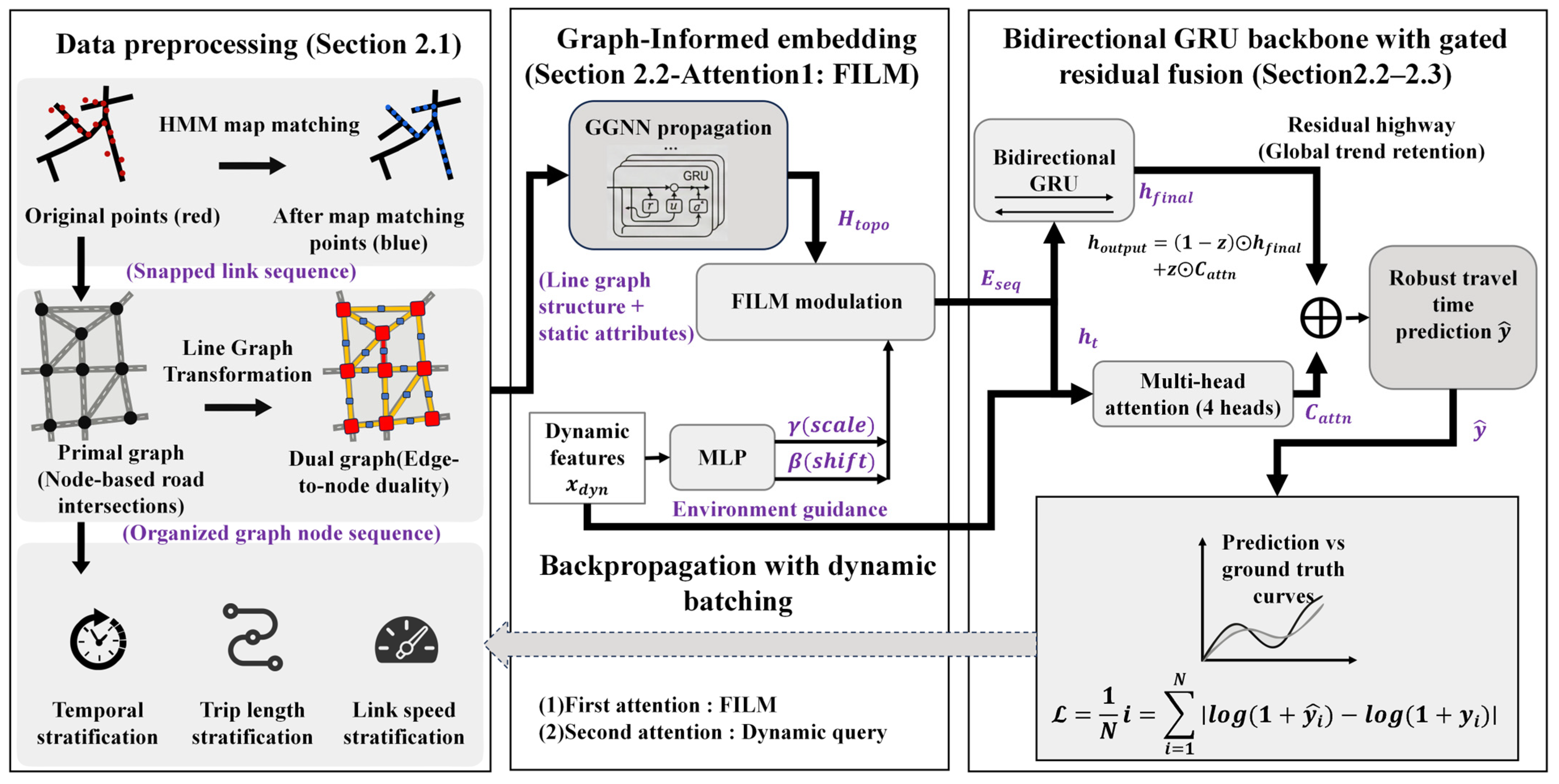
In this section, we propose a data-efficient and high-precision TTP framework named DAGRN. Unlike conventional sequence models that treat road segments as isolated tokens, DAGRN adopts a Graph-Informed Sequence Learning paradigm driven by a novel topology-temporal coordination mechanism. As illustrated in Figure 1, the framework comprises three tightly coupled stages: (1) a rigorous Data Engineering pipeline that transforms raw GPS logs into topological line graphs and explicitly stratified subsets (Section 2.1); (2) the DAGRN Core Architecture, which integrates a Gated Graph Neural Network (GGNN) with FiLM and a Gated Residual Fusion mechanism (Section 2.2); (3) a robust Optimization Strategy designed for training stability on variable-length sequences (Section 2.3).

To facilitate the formal mathematical description of the proposed method, the primary notations and their corresponding dimensions are summarized in

Table 1. Summary of Key Mathematical Notations.

Symbol	Description	Dimensions
G = (V, E)	The road network graph with nodes and edges	–
L(G) = (V′, E′)	The Line Graph (Dual Graph) where nodes represent road links	–
xstatic, xdyn	Static road attributes and dynamic temporal features	${\mathbb{R}}^{{\mathit{D}}_{\mathit{s}}},{\mathbb{R}}^{{\mathit{D}}_{\mathit{d}}}$
${\mathit{H}}_{\mathit{t}\mathit{o}\mathit{p}\mathit{o}}^{\left(\mathit{k}\right)}$	Topological embeddings updated at the k-th GGNN step	${\mathbb{R}}^{{\mathit{N}}_{\mathit{l}\mathit{i}\mathit{n}\mathit{k}}\times {\mathit{D}}_{\mathit{t}}}$
γ, β	Scale and shift parameters generated by FiLM	${\mathbb{R}}^{{\mathit{D}}_{\mathit{l}\mathit{i}\mathit{n}\mathit{k}}}$
Hrnn	The global hidden state of the Bi-GRU backbone	${\mathbb{R}}^{{2\mathit{D}}_{\mathit{h}}}$
Cattn	Context vector aggregated by Dynamic Query Attention	${\mathbb{R}}^{{2\mathit{D}}_{\mathit{h}}}$
$\widehat{y}$	Predicted travel time (log-transformed)	Scalar

Note: The symbol ‘–’ indicates that the item is a topological graph structure rather than a feature tensor with numerical dimensions.

.

2.1. Data Preprocessing and Graph Construction

High-fidelity spatio-temporal representation is the prerequisite for robust TTP. Raw GPS trajectories, however, suffer from intrinsic noise and topological disconnection. To address these challenges, we developed a systematic data engineering pipeline comprising noise correction, topological transformation, and a diversity-aware sampling strategy.

2.1.1. Line Graph Transformation

Conventional Graph Neural Networks (GNNs), as formalized by Scarselli et al. [28], typically represent intersections as nodes and road segments as edges. However, this design is suboptimal for TTP, as traffic dynamics—such as speed, volume, and congestion—are inherently associated with the segments rather than the intersections. Moreover, modeling dynamic edge attributes within standard GNN frameworks often leads to computational inefficiency.

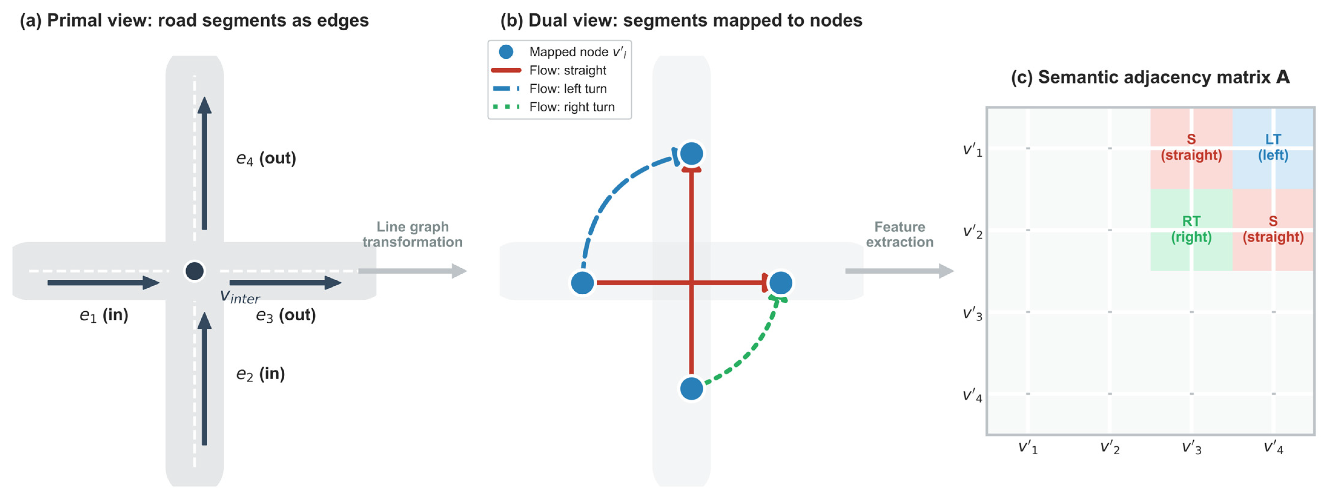
To overcome these limitations, we adopt a Line Graph transformation that inverts the conventional topology. Formally, given the primal road network G = (V, E), the Line Graph is defined as L(G) = (V′, E′), where each node v′ ∈ V′ corresponds to an edge e ∈ E in the primal graph. As illustrated in Figure 2a,b, this transformation maps each physical road segment to a graph node, enabling direct representation of traffic states. Studies such as Wang et al. [29] have emphasized that this explicit modeling of edge-to-edge connectivity allows for more effective capture of flow propagation.

Furthermore, to capture the heterogeneous nature of intersection movements, we extend the standard binary connections into a semantic adjacency matrix (Figure 2c). The dual graph explicitly differentiates flow types—such as straight, left-turn, and right-turn movements—assigning distinct topological semantics to the edges. Crucially, to ensure strict physical validity and establish a physics-aware structural prior, this directed adjacency matrix explicitly masks illegal real-world movements (e.g., forbidden left turns, one-way violations) with zero-weights. This guarantees that DAGRN propagates traffic states solely along legitimate, physically possible routes.

2.1.2. Trajectory Processing and Stratified Evaluation

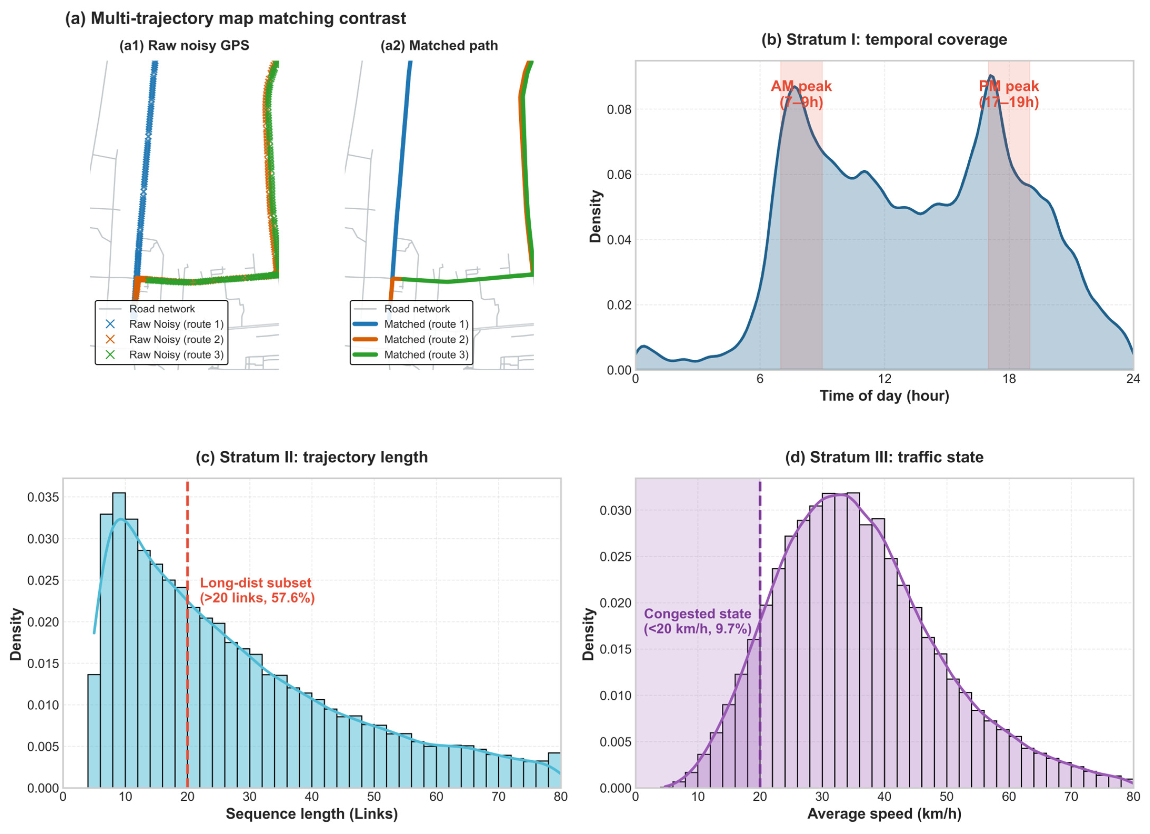
Trajectory Noise Correction. Since raw GPS data is inherently noisy and prone to signal drift, a map-matching process is essential before model ingestion. We implement a Hidden Markov Model (HMM)-based correction stage. As visualized in the split-view contrast of Figure 3a, the HMM calculates emission and transition probabilities to project scattered, noisy GPS points (Figure 3(a1)) onto the most topologically probable road segments (Figure 3(a2)), generating a clean “Snapped Link Sequence.” This ensures that the input to the Line Graph consists of physically valid network paths rather than disjointed coordinates.

Distribution Analysis and Stratified Sampling. Real-world traffic data typically exhibits an imbalanced distribution. Standard random sampling often leads to models that overfit to frequent patterns while failing on critical “corner cases.” To address this, we adopt a Stratified Sampling Strategy (illustrated in Figure 3b–d). Trajectories are categorized and balanced based on three dimensions:

• Temporal Stratification (Figure 3b): Captures volatility during peak hours (7–9 a.m., 17–19 p.m.).
• Spatial Stratification (Figure 3c): Specifically targets the spatial complexity by explicitly partitioning the long-distance trips (>20 links). According to our dataset distribution, this specific subset accounts for 57.6% of the total trajectories, ensuring the model effectively captures extended spatial dependencies without being biased by fragmented short trips.
• Traffic State Stratification (Figure 3d): Isolates congested flows where average speeds drop below 20 km/h. This cut-off is empirically derived and rigorously defines severe congestion scenarios, which constitute the most critical 9.7% of the overall speed distribution.

2.2. The DAGRN Architecture

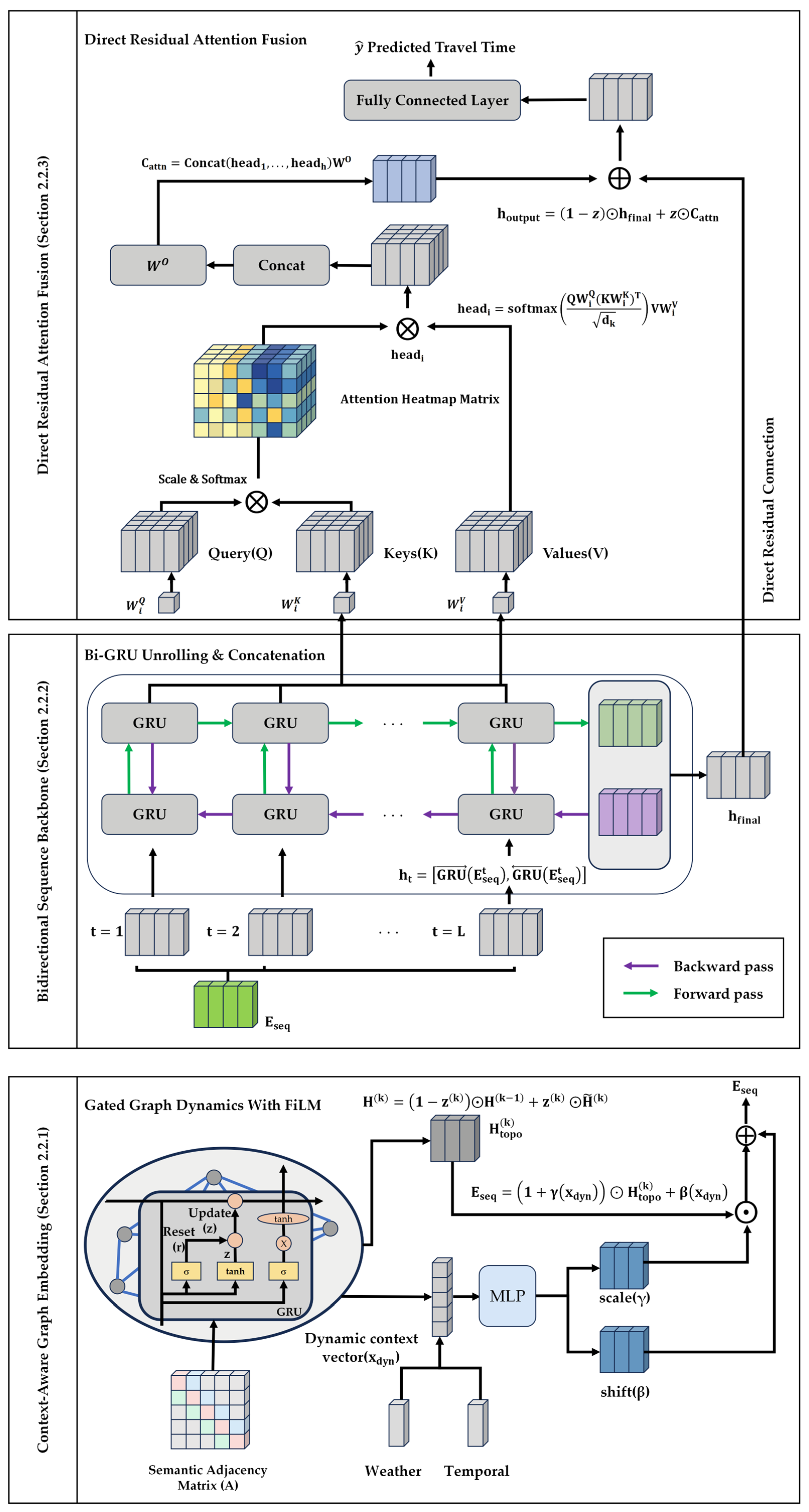
To enhance the accuracy and robustness of TTP under the data conditions described above, we propose the DAGRN framework. As illustrated in Figure 4, the model integrates three technically advanced components that form a Dual-Attentional mechanism: (1) Context-Aware Graph Embedding, where static topological features are dynamically modulated by environmental contexts via FiLM (serving as the First Attention mechanism); (2) Bidirectional Sequence Backbone, utilizing a Bi-GRU to capture for-ward and backward temporal dependencies; (3) Direct Residual Attention Fusion, which employs a Multi-Head Attention (the Second Attention) to pinpoint local fluctuations.

2.2.1. Gated Graph Dynamics with FiLM Modulation

To capture spatial dependencies among road segments, a GGNN is applied to the line graph. Let H⁽⁰⁾ denote the initial static features of road links. The node embeddings are iteratively updated using a GRU-based mechanism:

$${\mathit{H}}^{\left(\mathit{k}\right)}={\mathrm{G}\mathrm{R}\mathrm{U}}_{\mathrm{C}\mathrm{e}\mathrm{l}\mathrm{l}}\left({\mathit{H}}^{\left(\mathit{k}-\mathbf{1}\right)},\mathit{A}{\mathit{H}}^{\left(\mathit{k}-\mathbf{1}\right)}\mathit{W}\right)$$

(1)

where A is the adjacency matrix of the line graph and W is the learnable weight matrix.

However, static graph propagation fails to account for varying environmental conditions. To incorporate dynamic environmental context, we introduce the FiLM mechanism [30]. While standard GNNs often use fixed weights, recent works by Brockschmidt [31] have demonstrated that modulating layer activations with external context significantly improves adaptability. In DAGRN, a dynamic feature vector x_dyn is constructed by fusing temporal and environmental attributes. Specifically, weather data (e.g., rainfall, visibility) is sourced from the local meteorological bureau and temporally aligned with the trajectory start time via nearest-neighbor matching. Missing weather values are addressed via historical mean imputation. These environmental factors, along with discrete temporal features (hour of the day, day of the week), are strictly Min-Max normalized to a [0, 1] scale before being concatenated into x_dyn. This vector is then projected via a multi-layer perceptron to generate scale (γ) and shift (β) parameters:

$${\mathit{E}}_{\mathit{s}\mathit{e}\mathit{q}}=\left(1+\mathit{\gamma }\left({\mathit{x}}_{\mathit{d}\mathit{y}\mathit{n}}\right)\right)\odot {\mathit{H}}_{\mathit{t}\mathit{o}\mathit{p}\mathit{o}}^{\left(\mathit{K}\right)}+\mathit{\beta }\left({\mathit{x}}_{\mathit{d}\mathit{y}\mathit{n}}\right)$$

(2)

Crucially, this mechanism contributes to Cold-Start Robustness. By decoupling dynamic environmental factors (γ, β) from static topological structures, DAGRN learns universal environmental rules (e.g., rain induces global delays via β) that are transferable. This allows the model to generate conditioned embeddings even for sparse or unseen road segments by modulating their static attributes. To ensure training stability, the FiLM generator is initialized such that γ ≈ 0 and β ≈ 0.

2.2.2. Bidirectional Sequence Backbone

Once spatial embeddings are modulated, the system must capture the temporal evolution of traffic flow along the trajectory. We employ a Bidirectional Gated Recurrent Unit (Bi-GRU), which offers a performance comparable to LSTMs but with reduced computational complexity. The importance of bidirectional modeling—considering both the past history from the origin and the future context towards the destination—has been validated in recent adaptive traffic transformers like Chen et al. [32]. Following this intuition, the modulated sequence E_seq is processed in both directions:

$${\mathit{h}}_{\mathit{t}}=\left[\overrightarrow{\mathrm{G}\mathrm{R}\mathrm{U}}\left({\mathit{E}}_{\mathit{s}\mathit{e}\mathit{q}}^{\mathit{t}}\right),\overleftarrow{\mathrm{G}\mathrm{R}\mathrm{U}}\left({\mathit{E}}_{\mathit{s}\mathit{e}\mathit{q}}^{\mathit{t}}\right)\right]$$

(3)

The resulting hidden states {h₁, h₂, …, h_L} capture step-wise traffic dynamics. The final hidden state h_final, obtained by concatenating the last states from both forward and backward passes, serves as a global summary of the entire trajectory.

2.2.3. Multi-Head Attention Residual Fusion

A critical challenge identified in our data analysis (Section 2.1.2) is the presence of ultra-long trajectories (spanning thousands of links). In such scenarios, compressing the entire route into a single vector h_final creates a severe information bottleneck, and conventional concatenation strategies tend to increase dimensionality and destabilize training due to error accumulation. To resolve this, we design a Direct Residual Fusion mechanism that treats the backbone output as a stable baseline and uses attention as a sparse correction term.

Multi-Head Attention. First, we compute a context vector C_attn to retrieve fine-grained local details. This mechanism draws inspiration from the fundamental attention theory of Vaswani et al. [33] and aligns with recent meta-learning strategies for cold-start estimation [34]. Crucially, to jointly attend to information from different representation subspaces at different positions, we explicitly employ a Multi-Head Attention mechanism rather than a single-head formulation.

$${\mathit{C}}_{\mathit{a}\mathit{t}\mathit{t}\mathit{n}}=\mathrm{C}\mathrm{o}\mathrm{n}\mathrm{c}\mathrm{a}\mathrm{t}\left({\mathit{h}\mathit{e}\mathit{a}\mathit{d}}_{\mathbf{1}},\dots ,{\mathit{h}\mathit{e}\mathit{a}\mathit{d}}_{\mathit{h}}\right){\mathit{W}}^{\mathit{O}}$$

(4)

$${\mathit{h}\mathit{e}\mathit{a}\mathit{d}}_{\mathit{i}}=\mathrm{s}\mathrm{o}\mathrm{f}\mathrm{t}\mathrm{m}\mathrm{a}\mathrm{x}\left({\displaystyle \frac{\mathit{Q}{{\mathit{W}}_{\mathit{i}}^{\mathit{Q}}\left(\mathit{K}{\mathit{W}}_{\mathit{i}}^{\mathit{K}}\right)}^T}{\sqrt{d_k}}}\right)\mathit{V}{\mathit{W}}_{\mathit{i}}^{\mathit{V}}$$

(5)

In our configuration, the number of independent attention heads is set to h = 4. This multi-head design securely allows DAGRN to simultaneously capture multiple facets of localized traffic fluctuations (e.g., uncoordinated traffic signals and sudden lane merges) that a single-head mechanism might overlook.

Gated Residual Connection. Finally, instead of employing conventional concatenation or simplistic element-wise addition, we fuse the global backbone baseline h_final and the local attention correction C_attn via a dynamically regulated gated residual connection. Let z = σ ([|C_attn||h_final||x_dyn|]) be the fusion gate, the final representation is computed as:

$${\mathit{h}}_{\mathit{o}\mathit{u}\mathit{t}\mathit{p}\mathit{u}\mathit{t}}=\left(1-\mathit{z}\right)\odot {\mathit{h}}_{\mathit{f}\mathit{i}\mathit{n}\mathit{a}\mathit{l}}+\mathit{z}\odot {\mathit{C}}_{\mathit{a}\mathit{t}\mathit{t}\mathit{n}}$$

(6)

$$\widehat{y}={\mathit{W}}_{\mathit{o}\mathit{u}\mathit{t}}\left(h_{output}\right)+b_{out}$$

(7)

This gated structure extends the residual learning paradigm. It allows the model to utilize h_final as a robust global prior while dynamically shifting the focus toward C_attn during extreme localized fluctuations via the gate z.

2.3. Optimization and Training Strategy

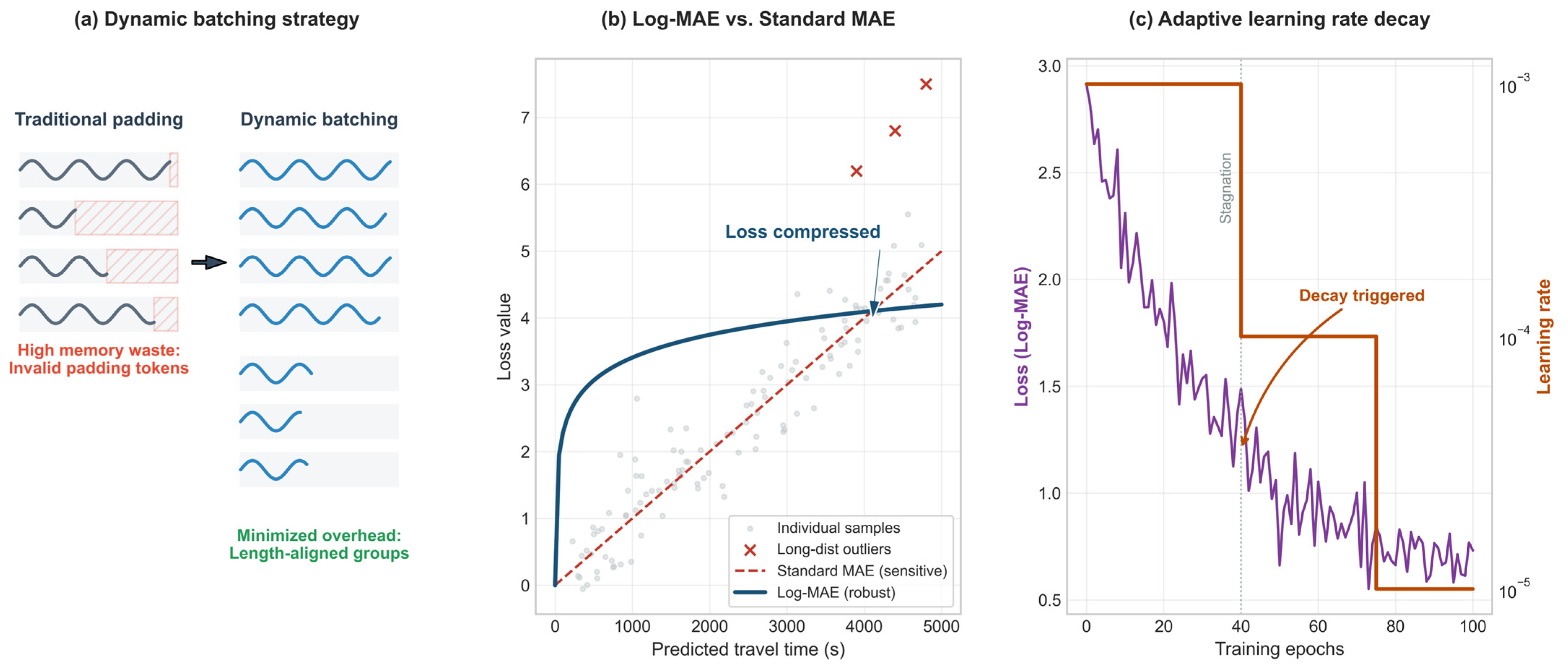
The training process of DAGRN is governed by a robust optimization engine (Figure 5) explicitly designed to handle the variability and sparsity of trajectory data described in Section 2.1.

Robust Objective Function (Log-MAE). Traditional Mean Squared Error (MSE) loss is highly sensitive to outliers, particularly for long-distance trips. To mitigate this, we employ the Mean Absolute Error (MAE) on a logarithmic scale. The logarithmic transformation compresses the target range, proportionally balancing the contribution of short and long trips as follows:

$$\mathcal{L}={\displaystyle \frac{1}{N}}i=\sum _{i=1}^N\mid log(1+\widehat{y_i})-log(1+y_i)\mid$$

(8)

where y_i and $\widehat{{\mathit{y}}_{\mathit{i}}}$ denote the ground truth and predicted travel times, respectively.

Dynamic Batching & Adaptive Scheduling. Handling variable-length trajectory sequences poses computational challenges. Instead of padding all sequences to the global maximum length (which severely wastes GPU memory), we implement a dynamic batching strategy (Figure 5a), grouping sequences of similar lengths to minimize invalid padding tokens. Furthermore, to facilitate stable convergence, we utilize the AdamW optimizer coupled with a plateau-based scheduler (ReduceLROnPlateau implemented in PyTorch v2.3, Figure 5c), which dynamically decays the learning rate upon validation loss stagnation to allow fine-grained weight adjustment.

3. Experiments and Analysis

In this section, we conduct a comprehensive evaluation of the proposed DAGRN framework. Unlike conventional studies that rely on massive historical logs to train highly parameterized deep learning models, our experimental design explicitly addresses a critical bottleneck in real-world intelligent transportation deployment: the cold-start problem. We rigorously evaluate the model’s ability to achieve high-precision forecasting utilizing a severely constrained dataset (comprising merely 2000 trajectories). This setup aims to unequivocally verify whether the proposed physics-aware structural priors and topology-temporal coordination mechanisms can ensure robust generalization in data-scarce regimes where traditional frameworks succumb to overfitting.

3.1. Experimental Setup

3.1.1. Dataset and Evaluation Metrics

The experiments utilize real-world vehicle trajectory data collected from Wuxi City. To rigorously simulate a data-scarce edge deployment environment, we constructed a sparse dataset containing only 2000 high-quality trajectories after the HMM kinematic filtering described in Section 2.1. The dataset is partitioned into Training (70%), Validation (10%), and Testing (20%) sets based exclusively on chronological order, fundamentally preventing the future information leakage that frequently compromises spatio-temporal forecasting evaluations.

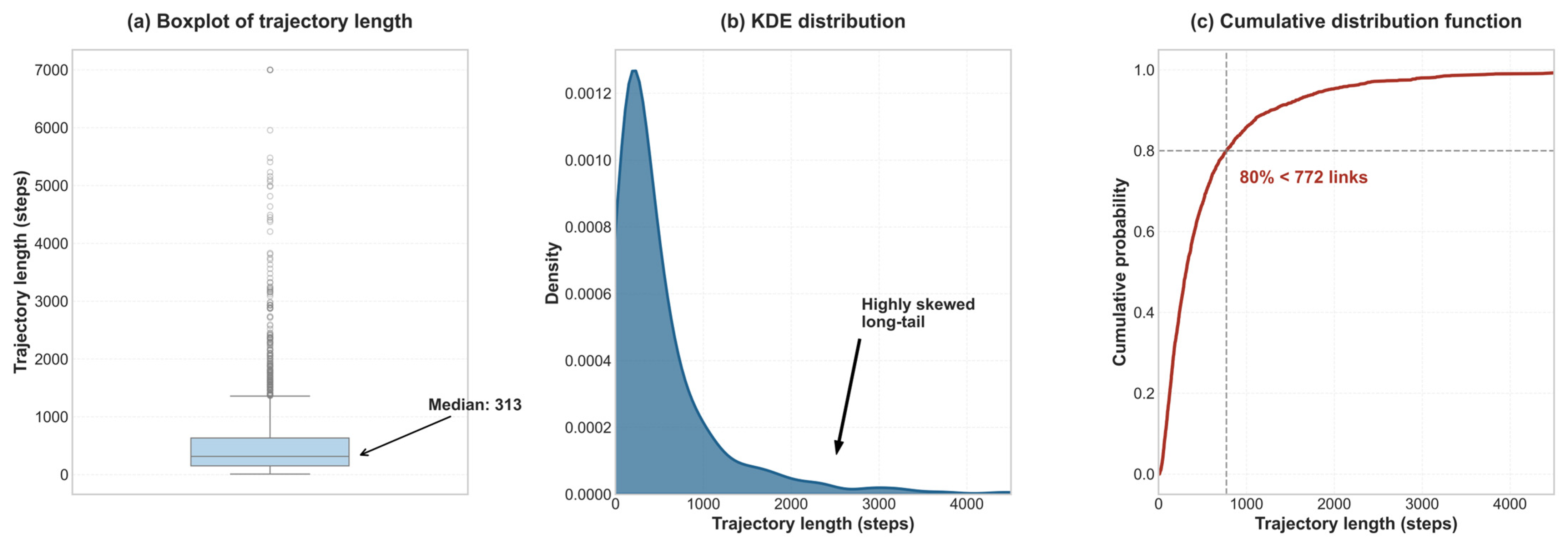
We thoroughly analyzed the length distribution of this sparse dataset to quantify the inherent complexity of the prediction task. As visualized in Figure 6, the data exhibits a highly skewed long-tail pattern. Specifically, the boxplot (Figure 6a) highlights the prevalence of short trips, with a median length of 313 steps, alongside numerous extreme outliers. The KDE distribution (Figure 6b) further illustrates the high density in the low-step regime and the sustained sparse tail. Finally, the cumulative distribution function (CDF) (Figure 6c) confirms the distribution characteristics, revealing that 80% of the trajectories contain fewer than 772 links, while a critical subset of extreme cases extends toward 7000 links.

All models were implemented using the PyTorch 2.3 framework on a workstation equipped with an NVIDIA GeForce RTX 4070Ti GPU. The DAGRN model was configured with a hidden dimension of 64, 3 GCN layers, and 4 attention heads. The model was trained using the AdamW optimizer with a dynamic learning rate scheduler (ReduceLROnPlateau) and optimized via a Log-L1 Loss function. The specific parameter settings for DAGRN are systematically detailed in

Table 2. Hyperparameter Settings.

Parameter Category	Parameter Name	Value
Model Architecture	ID Embedding Dimension	32
	Hidden Dimension (RNN/GCN)	64
	Number of GCN Layers	3
	Attention Heads	4
Training Strategy	Optimizer	AdamW
	Learning Rate (lr)	1 × 10−3 (ReduceLROnPlateau)
	Batch Size	32
	Loss Function	L1 Loss (Log-Space)
	Regularization (Dropout)	0.3

.

To evaluate performance quantitatively, four standard metrics are employed: Mean Absolute Error (MAE), Root Mean Squared Error (RMSE), Mean Absolute Percentage Error (MAPE), and the Coefficient of Determination (R²). Additionally, to assess robustness in extreme conditions, we report Congested-MAPE, which is calculated exclusively on the top 10% of trips with the lowest average speeds. The formulas are defined as follows:

$$MAE = {\displaystyle \frac{1}{N}}\sum _{i=1}^N\left|\widehat{y_i}-y_i\right|$$

(9)

$$\begin{array}{c}RMSE =\sqrt{{\displaystyle \frac{1}{N}}{\displaystyle \sum _{i=1}^N}{\left(\widehat{y_i}-y_i\right)}^2}\end{array}$$

(10)

$$\begin{array}{c}MAPE={\displaystyle \frac{1}{N}}{\displaystyle \sum _{i=1}^N}\left|{\displaystyle \frac{\widehat{y_i}-y_i}{y_{\mathrm{i}}}}\right|\times 100\%\end{array}$$

(11)

$$R^2=1-{\displaystyle \frac{{\sum }_{i=1}^N{\left(\widehat{y_i}-y_i\right)}^2}{{\sum }_{i=1}^N{\left(\overline{y_i}-y_i\right)}^2}}$$

(12)

where $\widehat{y_i}$ and $y_i$ denote the ground truth and predicted travel times, respectively, and $\overline{y_i}$ represents the mean of the ground truth.

3.1.2. Data Stratification for Robustness Analysis

We benchmark DAGRN against 12 representative baselines, categorized into three distinct groups to ensure a comprehensive comparison against both fundamental and state-of-the-art frameworks:

• Sequence and Temporal Models. We evaluate fundamental recurrent architectures, including LSTM and GRU. Recent works [35] have highlighted their continued relevance for handling missing data in sparse environments. We also include Temporal Convolutional Networks (TCNs) [36] and attention-enhanced variants (Attn-GRU).
• Spatio-Temporal GNNs. We include advanced graph-based architectures that fuse spatial convolution with recurrent units, namely GCN-GRU, TAGCN-GRU, GAT-LSTM [37], and Graph WaveNet. Additionally, Additionally, we evaluate Adaptive-GGNN as a representative baseline for adaptive graph recurrent networks [38].
• Trajectory-Specific Models. To benchmark against the cutting edge tailored specifically for travel time estimation, we utilize DeepTTE [39], GraphTTE [40], and GSTA [41].

3.2. Comparative Analysis

3.2.1. Performance Analysis on Sparse Data

Table 3. Comprehensive Evaluation of Baseline Models (2k).

Variant	MAE (s)	RMSE (s) (Long_RMSE)	MAPE (%)	R2	Peak_ RMSE	Congested _RMSE	Peak_R2	Congested_R2
LSTM	488.707	869.995	49.429	0.335	787.804	541.168	0.320	−0.017
GAT-LSTM	433.722	783.089	44.049	0.461	824.820	485.621	0.255	0.180
DeepTTE	372.135	665.039	41.343	0.611	696.314	458.929	0.469	0.268
TCN	347.091	628.200	31.692	0.653	572.440	468.618	0.641	0.237
GCN-GRU	337.011	623.575	32.493	0.658	627.352	464.373	0.569	0.250
Attn-GRU	336.483	594.758	31.350	0.689	545.636	390.303	0.674	0.470
GraphTTE	351.558	592.563	33.413	0.691	554.076	490.899	0.664	0.162
Graph WaveNet	293.099	556.202	28.436	0.728	480.407	324.734	0.747	0.633
GRU	293.933	548.852	31.728	0.735	550.127	370.225	0.668	0.523
TAGCN-GRU	280.476	518.486	30.353	0.763	506.339	399.568	0.719	0.445
GSTA	285.916	485.312	30.902	0.793	467.265	424.048	0.761	0.375
Adaptive-GGNN	251.533	482.059	26.623	0.795	438.870	365.422	0.789	0.536
DAGRN (Ours)	225.152	415.485	24.285	0.848	401.400	377.308	0.823	0.505

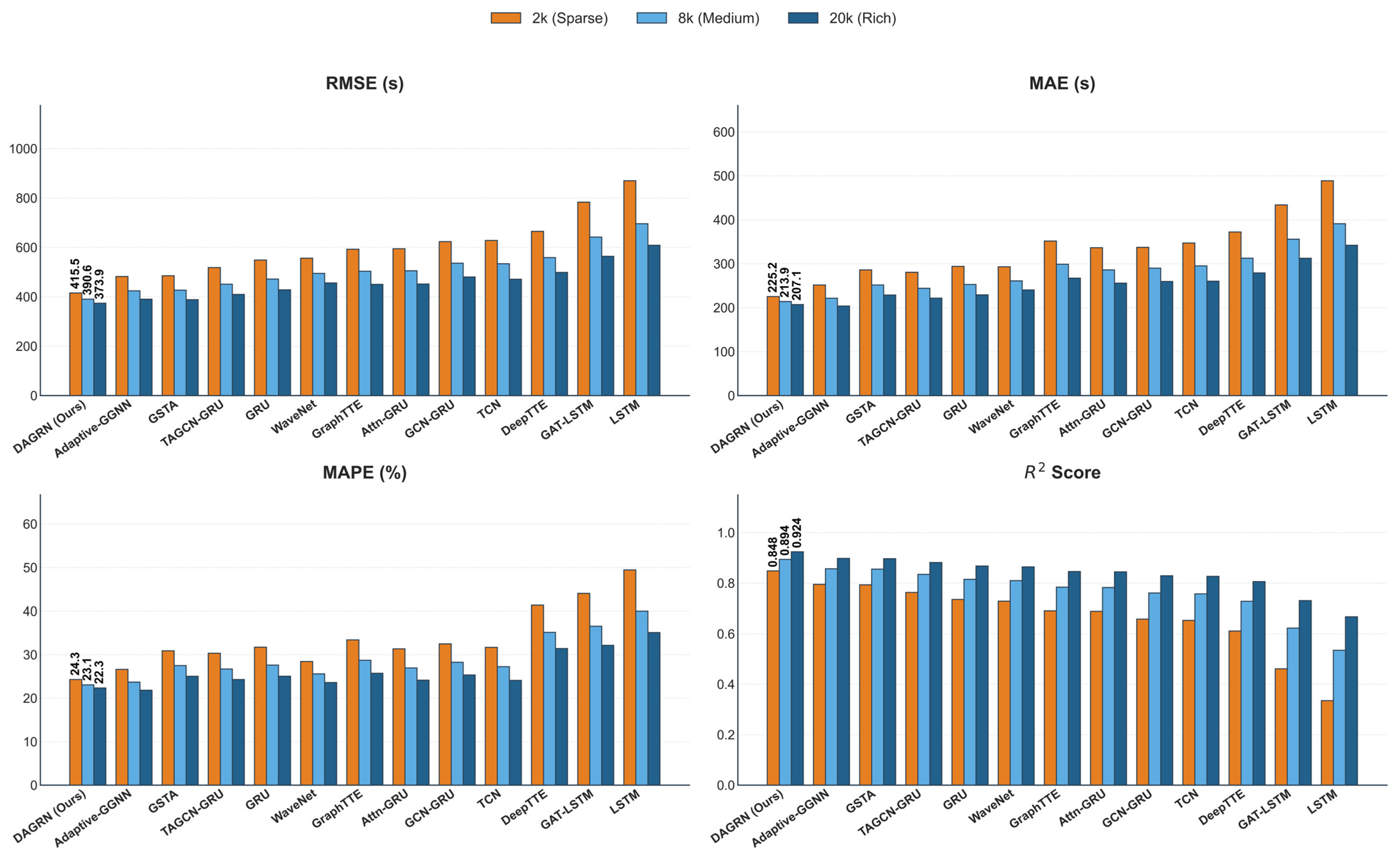
Note: Bold values indicate the best performance in each column.

comprehensively illustrates the multi-dimensional performance of all models evaluated on the sparse data regime. Complementing this, Figure 7 provides a visual benchmark of the proposed DAGRN against the 12 baseline models across four standard evaluation metrics under sparse (2k), medium (8k), and rich (20k) data regimes.

In the critical cold-start regime (2k trajectories), DAGRN consistently establishes superiority across all overall evaluation metrics. Specifically, DAGRN achieves a state-of-the-art RMSE of 415.485 s and an R² of 0.848, significantly outperforming both the strongest spatio-temporal baselines (e.g., Adaptive-GGNN) and generic sequence models. Notably, while sequence-based models exhibit sharp error spikes due to their inability to leverage physical road topology, highly parameterized models like Graph WaveNet also struggle in aggregate forecasting (RMSE: 556.202 s), displaying clear signs of overfitting. This phenomenon aligns directly with recent reviews by Jiang and Luo [42], which emphasized that highly parameterized GNNs require abundant historical data to stabilize their adaptive adjacency matrices. Similarly, Jin et al. [43] highlighted that without explicit structural priors, dynamic graph models tend to learn spurious correlations when training samples are sparse.

Conversely, DAGRN’s exceptional R² score confirms that the explicitly constructed Line Graph topology acts as a robust, physics-aware inductive bias, perfectly compensating for the lack of massive historical data. This finding strongly resonates with Pan et al. [44], who demonstrated that explicitly encoded structural priors are essential for robust prediction in few-shot traffic scenarios.

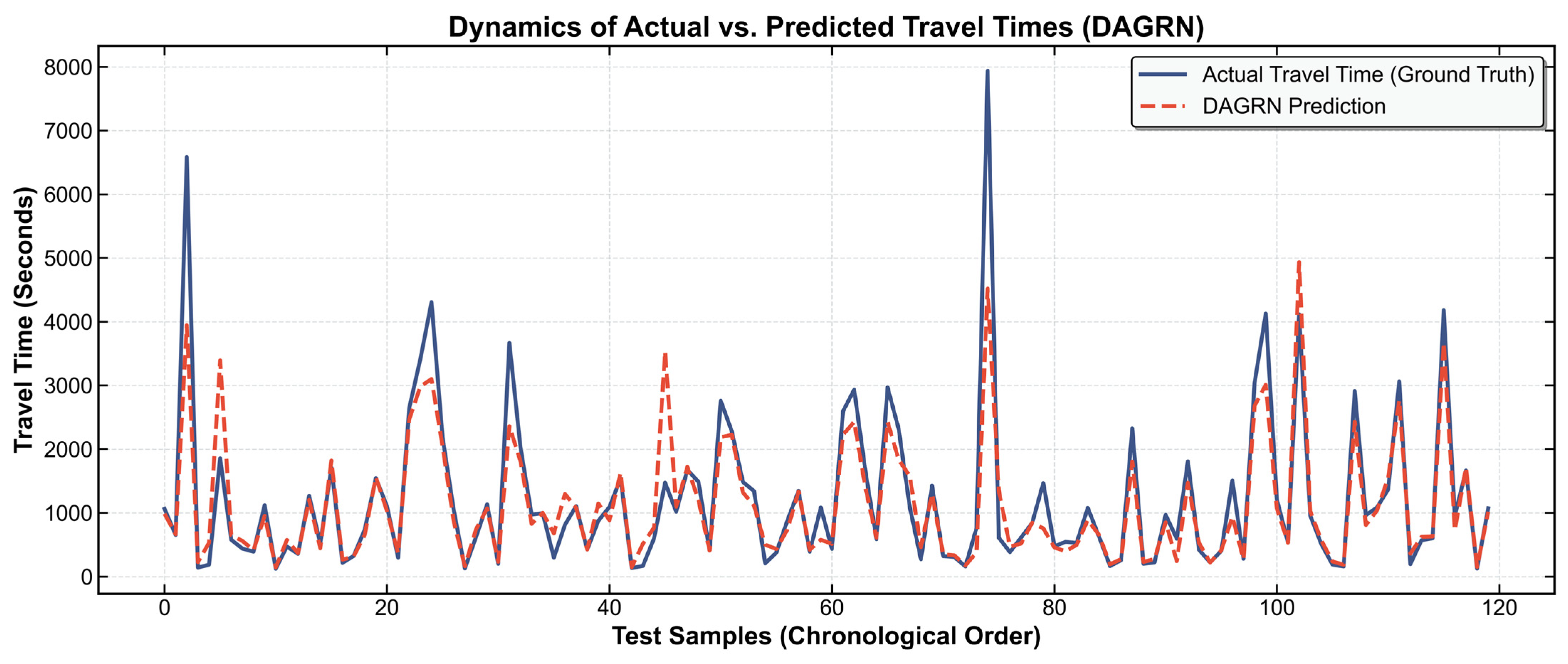
To explicitly illustrate the model’s dynamic forecasting capability—a critical metric for real-world dispatching systems—Figure 8 visualizes the dynamics of actual versus predicted travel times for a representative sequence of test trajectories.

As depicted in Figure 8, DAGRN not only accurately captures the baseline travel time but tightly tracks sudden, highly volatile peaks caused by transient congestion. Unlike baseline models that tend to produce smoothed, delayed estimates during abrupt traffic waves, DAGRN ensures highly responsive and precise predictions, unequivocally demonstrating its practical value for ITS deployment.

3.2.2. Robustness in Challenging Scenarios

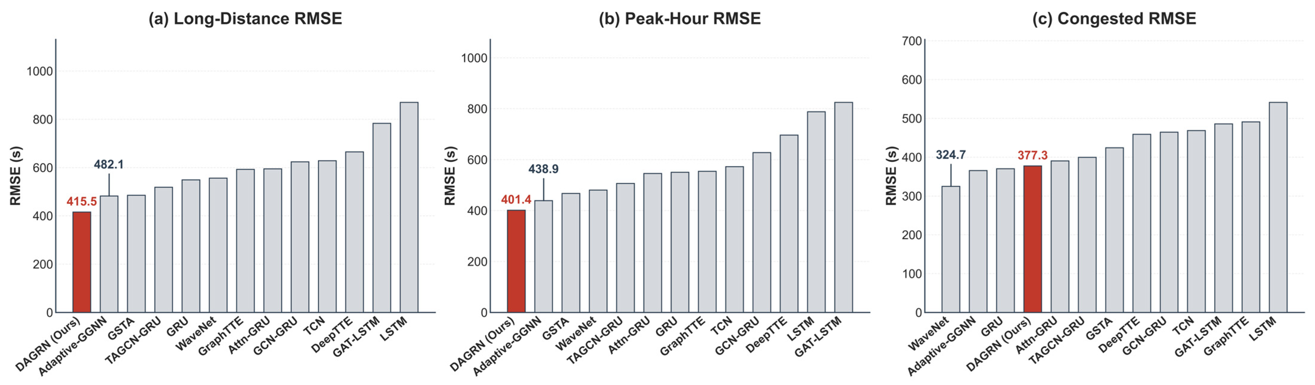
Beyond aggregate performance, robust TTP requires stability across diverse stress conditions. As illustrated in Figure 9, we decomposed model performance into three distinct challenging scenarios:

(a)

Long-Distance Trips (>20 links): Longer trajectories exponentially amplify cumulative prediction errors. DAGRN mitigates this error accumulation via its Gated Residual Fusion mechanism, delivering consistently low RMSE and actively avoiding the sharp error spikes observed in baselines.

(b)

Peak-Hour Traffic: During peak hours (07:00–09:00 and 17:00–19:00), traffic patterns exhibit heightened volatility. DAGRN’s Multi-Head Attention effectively captures these localized fluctuations, maintaining stable Peak-Hour RMSE despite limited training samples.

(c)

Congested Regimes: In severely congested conditions (defined as the top 10% slowest trips), prediction becomes highly sensitive to minor speed variances. DAGRN sustains highly competitive Congested-RMSE and MAPE metrics, yielding fewer extreme outliers than most baselines, thereby indicating strong robustness against traffic degradation.

These three scenarios represent complementary stress conditions—spatial, temporal, and state-based—and jointly validate DAGRN’s stability. While specific baselines (e.g., Graph WaveNet) may achieve slightly lower errors in isolated congested cases, they suffer from severe performance degradation in long-distance and peak-hour regimes. In contrast, DAGRN maintains an exceptionally balanced and superior performance across all stress conditions, supporting its adaptability to non-stationary traffic distributions.

3.3. Ablation Study

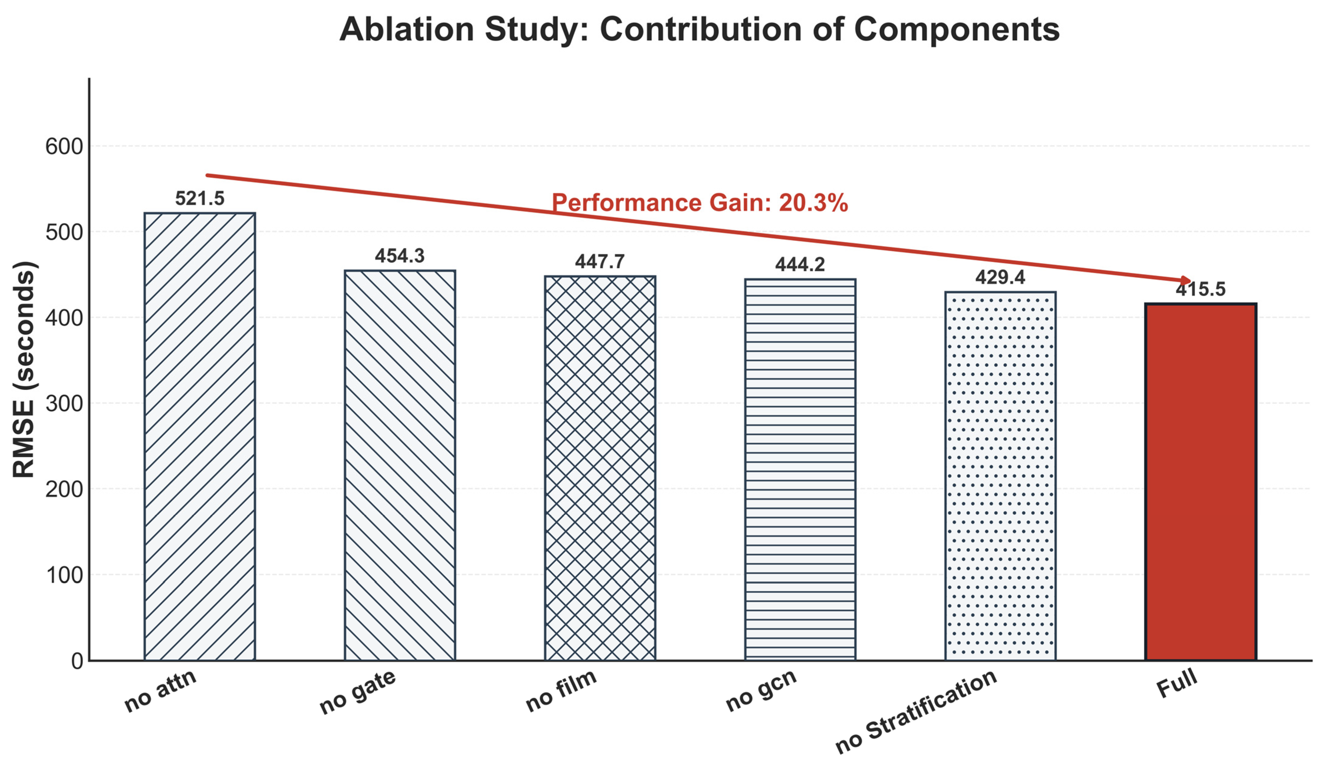
To empirically isolate the contribution of each architectural innovation, we conducted a rigorous ablation study. The quantitative results are detailed in

Table 4. Ablation Study Quantitative Results (2k).

Variant	MAE (s)	RMSE (s)	MAPE (%)	R2	Long_RMSE (s)	Peak_RMSE (s)	Congested_RMSE (s)
DAGRN_no_gcn	232.441	444.166	26.384	0.826	444.166	447.681	345.409
DAGRN_no_attn	287.816	521.495	32.783	0.761	521.495	493.713	429.464
DAGRN_no_Stratification	239.268	429.366	24.468	0.838	429.366	426.544	431.177
DAGRN_no_film	230.421	447.665	25.428	0.823	447.665	480.111	352.867
DAGRN_no_gate	239.996	454.289	27.593	0.818	454.289	473.743	357.867
DAGRN_Full	225.152	415.485	24.285	0.848	415.485	401.400	377.308

Note: Bold values indicate the best performance in each column.

and Figure 10. This sparse data regime best isolates the effectiveness of our structural design from data-driven overfitting.

• Impact of Data Stratification (w/o Stratification): Training the model on a randomly sampled dataset without stratification exposes a dangerous long-tail bias, with the RMSE significantly increasing from 415.49 s to 429.37 s. This degradation is most pronounced in the severely congested regime, where the Congested-RMSE drastically spikes from 377.31 s to 431.18 s. This explicitly validates that our spatial stratification strategy effectively prevents the model from overwhelmingly overfitting to abundant, trivial short trips, guaranteeing robust generalization on complex, volatile trajectories.
• Impact of Topological Structure (w/o GCN): Removing the GCN module causes a significant performance drop, with the RMSE increasing to 444.17 s and R2 dropping to 0.826. This unequivocally confirms that the Line Graph topology serves as a foundational regularizer. As noted by Ji et al. [45], incorporating physical connectivity constraints is essential when training data is insufficient to learn the underlying manifold.
• Impact of Dynamic Context (w/o FiLM): The removal of FiLM modulation increases the RMSE to 447.67 s. This confirms that static topological embeddings alone are insufficient; the graph structure must be dynamically modulated by environmental contexts to prevent systematic bias under varying weather or temporal conditions.
• Impact of Attention and Fusion (w/o Attn, w/o Gate): The gating mechanism is structurally indispensable, as its removal (w/o Gate) causes the overall RMSE to regress to 454.289 s. More critically, the complete removal of the Multi-Head Attention module (w/o Attn) precipitates the most severe performance collapse across the entire ablation study, with the overall RMSE skyrocketing to 521.495 s. Furthermore, without the environment-guided local attention, the model loses its ability to capture intersection delays, causing the Congested-RMSE to surge to 429.464 s.

Trade-off Analysis in Extreme Regimes: It is worth noting that while some simplified variants (e.g., w/o GCN or w/o Gate) exhibit numerically lower errors in the isolated Congested subset (e.g., 345.409 s and 357.867 s, respectively), this is a false positive caused by systematic over-prediction biases. By losing structural constraints, these degraded models blindly predict longer travel times, which coincidentally fits the extreme tail-end samples but triggers catastrophic failures in the Overall and Peak-Hour metrics. DAGRN_Full achieves the optimal architectural balance, aggressively suppressing overall errors while maintaining highly competitive accuracy in extreme congestion.

3.4. Parameter Sensitivity Analysis

To rigorously evaluate the robustness of DAGRN and identify the optimal hyperparameter configuration, we conducted a comprehensive sensitivity analysis using the Control Variate Method on the 2k dataset. We established a default baseline and varied one parameter at a time. The quantitative results are summarized in

Table 5. Sensitivity analysis results of DAGRN under different hyperparameter settings (2k).

Parameter Changed	Hidden Dim	Dropout Rate	Learning Rate	GCN Iter	Attention Heads	Batch Size	RMSE (s)	MAE (s)
hidden_dim = 32	32	–	–	–	–	–	476.20	246.26
hidden_dim = 64	64	–	–	–	–	–	430.75	220.75
hidden_dim = 128	128	–	–	–	–	–	402.59	221.48
dropout_rate = 0.2	–	0.2	–	–	–	–	401.95	216.12
dropout_rate = 0.5	–	0.5	–	–	–	–	433.74	238.63
dropout_rate = 0.7	–	0.7	–	–	–	–	534.12	291.17
lr = 0.0005	–	–	0.0005	–	–	–	466.16	232.73
lr = 0.001	–	–	0.001	–	–	–	399.92	217.10
lr = 0.005	–	–	0.005	–	–	–	457.78	263.71
gcn_iter = 1	–	–	–	1	–	–	467.34	241.53
gcn_iter = 2	–	–	–	2	–	–	446.32	229.24
gcn_iter = 3	–	–	–	3	–	–	444.81	232.15
attention_heads = 2	–	–	–	–	2	–	425.65	220.82
attention_heads = 4	–	–	–	–	4	–	419.26	225.66
attention_heads = 8	–	–	–	–	8	–	491.83	252.03
batch_size = 32	–	–	–	–	–	32	399.89	214.22
batch_size = 64	–	–	–	–	–	64	442.78	228.58
batch_size = 128	–	–	–	–	–	128	479.08	245.85

Note: Bold values indicate the best performance in each column. The symbol ‘–’ indicates that the parameter was maintained at its default baseline value.

.

• Impact of Model Capacity: Increasing the hidden dimension from 32 to 128 yields a consistent performance boost, suggesting the model benefits from a larger representational capacity to capture complex topological dependencies. However, the improvement plateaus, indicating that a dimension of 64 provides a cost-effective balance for practical deployment. This observation is consistent with Di et al. [46], who suggested that compact representations are often more robust for traffic state estimation under data constraints.
• Impact of Regularization: The dropout rate exhibits a distinct preference for lower values. Contrary to the common assumption that high dropout is essential for small datasets, a rate of 0.2 achieved optimal performance, whereas increasing it to 0.5 or 0.7 significantly deteriorated the RMSE. This indicates that the structural priors introduced by our Line Graph and FiLM modules actively function as strong regularizers; consequently, aggressive dropout merely disrupts the learning of subtle traffic patterns.
• Impact of Optimization Settings: A learning rate of 0.001 emerges as the most stable optimization parameter. Notably, a smaller batch size of 32 significantly outperforms larger batches (e.g., 128). This phenomenon is highly characteristic of data-scarce regimes, where smaller batches provide more frequent weight updates and introduce stochastic noise that assists the optimizer in escaping sharp local minima.

3.5. Computational Complexity Analysis

While the Line Graph transformation inherently increases the number of graph nodes (by mapping primal edges to dual nodes), the overall computational overhead remains highly efficient for targeted cold-start scenarios. On the 2k dataset, the average training time is approximately 5 s per epoch (measured on an NVIDIA RTX 4070Ti).

This exceptional efficiency ensures that DAGRN can be rapidly retrained and seamlessly deployed in resource-constrained edge computing environments. Unlike recent generative approaches such as DiffSTG [47] or PriSTI, which require iterative denoising steps during inference resulting in prohibitive latency, DAGRN maintains a deterministic and lightweight forward pass. Similarly, complex recurrent graph models like MSDR [48] involve heavy computational overhead. In stark contrast, DAGRN achieves a highly practical balance between predictive accuracy and deployment efficiency.

4. Discussion

The empirical results presented in Section 3 unequivocally demonstrate the effectiveness of the DAGRN framework within the challenging cold-start regime. To fully contextualize these findings, we discuss the underlying mechanisms, acknowledge inherent methodological limitations, and position DAGRN within the broader landscape of recent deep learning advancements.

Structural Priors vs. Data-Driven Induction. State-of-the-art architectures such as PDFormer and DSTAGNN rely heavily on data-driven graph structure learning. While theoretically powerful, this inductive approach requires massive data to converge. In our severely constrained 2k dataset, such highly parameterized models tend to learn spurious correlations, leading to the overfitting observed in the baselines. DAGRN elegantly circumvents this by explicitly encoding the physics-aware Line Graph as a hard structural prior. This design choice corroborates the arguments of Wang et al. [49] and Züfle et al. [50], who demonstrated that knowledge-driven topologies (e.g., physical road connectivity) are significantly more reliable than data-driven graphs when spatial observability is low. By enforcing strict physical connectivity, DAGRN radically reduces the hypothesis space, preventing mathematical degradation.

Pragmatic Efficiency vs. Generative Overhead. Recent works have increasingly employed generative paradigms, such as Spatial-Temporal ODEs [51] or Diffusion models, to impute missing traffic patterns. While effective for offline analysis, they introduce prohibitive computational latency during iterative inference. DAGRN offers a pragmatic, deployment-ready alternative: utilizing FiLM to dynamically adapt the static topological graph to varying environmental contexts. This achieves robustness comparable to generative methods but maintains a deterministic and lightweight forward pass, fulfilling the stringent low-latency requirements of real-time ITS edge computing.

Positioning in the Broader Landscape. The field of traffic prediction has expanded rapidly, as categorized by recent comprehensive benchmarks and surveys. While Transformer variants [52] and Hierarchical GCNs [53] show immense promise in data-rich scenarios, our comparative analysis confirms they lack the necessary inductive biases for data-scarce tasks. Recently, researchers have proposed dual-view graph approaches [54] and attention-based GNNs such as ASTGCN [55] to enhance robustness. DAGRN differentiates itself from these works by specifically targeting the cold-start data constraint through a dual Line Graph transformation and multi-head localized attention, rather than merely escalating overall network complexity.

Methodological Boundaries and Micro-Level Complexities. Despite its superior efficiency, DAGRN fundamentally operates at a macroscopic and mesoscopic topological level, which inherently bounds its predictive precision. Real-world traffic volatility is frequently driven by unobservable microscopic complexities. For instance, as a macro-level GNN, DAGRN does not currently capture explicit vehicle-to-vehicle (V2V), vehicle-to-pedestrian (V2P), or vehicle-to-everything (V2X) interactions, nor does it explicitly account for fine-grained environmental conditions such as road lighting levels or detailed weather micro-climates. Capturing these highly stochastic, micro-level dynamics and unscheduled traffic signal preemptions remains an unresolved frontier for graph-based frameworks. Furthermore, DAGRN relies on a predefined, static road network topology [56], making it less adaptive to sudden structural disruptions (e.g., unexpected road closures or construction).

Crucially, our robustness analysis reveals a specific empirical boundary: in severely congested regimes, DAGRN was marginally outperformed by highly parameterized, Transformer-based WaveNet architectures. While DAGRN excels in maintaining balanced stability across all general scenarios, Transformer-based mechanisms demonstrate a unique advantage in modeling extreme, long-range temporal correlations and bottleneck delays during severe traffic degradation. To systematically overcome this limitation, our immediate future work will explore hybridizing DAGRN’s physics-aware structural priors with advanced Transformer-based temporal modules. We aim to evolve the current framework into a Multi-Scale DAGRN (MS-DAGRN), which will be specifically designed to dynamically capture both macro-level spatial topologies and micro-level temporal congestion variations. Acknowledging these limitations not only delineates the operational boundaries of the proposed framework but also establishes a clear, actionable trajectory for next-generation intelligent transportation models.

5. Conclusions

This study addresses the persistent dilemma of deploying high-fidelity TTP models within data-scarce, cold-start environments. Conventional deep learning architectures, while powerful, typically falter in such regimes due to their heavy reliance on massive historical logs to implicitly learn spatial dependencies. To bridge this critical gap, we proposed DAGRN, a robust framework that shifts the paradigm from purely data-driven induction toward Graph-Informed Sequence Learning. By integrating a physics-aware Line Graph-based GGNN to explicitly model edge-to-edge connectivity, and employing FiLM to dynamically inject environmental priors, DAGRN effectively compensates for the lack of extensive training samples. Extensive empirical evaluations on a highly sparse dataset (merely 2000 trajectories) demonstrate that DAGRN achieves a state-of-the-art RMSE of 415.485 s. Specifically, it reduces prediction error by 13.8% compared to the strongest dynamic graph baseline (Adaptive-GGNN) and by 24.3% compared to the most competitive generic sequence models. Furthermore, our ablation studies explicitly confirm that the structural priors provided by the Line Graph, coupled with the localized capture capability of the Multi-Head Attention mechanism, act as critical regularizers, preventing the overfitting observed in over-parameterized architectures. Crucially, DAGRN achieves this superior accuracy while maintaining high computational efficiency, avoiding the latency bottlenecks of recent generative imputation methods.

Our research opens several strategic avenues for future exploration. First, to overcome the aforementioned macroscopic limitations and enhance predictive precision in severe congestion, future work will evolve the current architecture into a Multi-Scale DAGRN (MS-DAGRN). This will involve hybridizing DAGRN with Transformer-based temporal modules and microscopic traffic simulators (e.g., SUMO or VISSIM). This synergistic approach will allow macro-level topological predictions to be calibrated by micro-level behavioral simulations, effectively bridging the gap between mathematical forecasting and real-world traffic wave dynamics. Second, recognizing that static graphs cannot capture sudden topological changes, we plan to incorporate dynamic discrete graph evolution techniques to enable real-time structural updates during inference. Finally, to enhance the transparency of ITS decision-making, we aim to explore the integration of Large Language Models (LLMs). By coupling DAGRN’s numerical precision with the semantic reasoning of LLMs, we envision a system capable of providing natural language diagnostic insights into predicted travel time fluctuations, thereby transforming opaque AI outputs into human-readable traffic intelligence.

References

1. Billings, D.; Yang, J.-S. Application of the ARIMA models to urban roadway travel time prediction—A case study. In Proceedings of the 2006 IEEE International Conference on Systems, Man and Cybernetics, Taipei, Taiwan, 8–11 October 2006; IEEE: Piscataway, NJ, USA, 2006; pp. 2529–2534. [Google Scholar] [CrossRef] [Scilit]
2. Guin, A. Travel time prediction using a seasonal autoregressive integrated moving average time series model. In Proceedings of the 2006 IEEE Intelligent Transportation Systems Conference, Toronto, ON, Canada, 17–20 September 2006; IEEE: Piscataway, NJ, USA, 2006; pp. 493–498. [Google Scholar] [CrossRef] [Scilit]
3. Yin, X.; Wu, G.; Wei, J.; Shen, Y.; Qi, H.; Yin, B. Deep learning on traffic prediction: Methods, analysis, and future directions. IEEE Trans. Intell. Transp. Syst. 2022, 23, 4927–4943. [Google Scholar] [CrossRef] [Scilit]
4. Wu, C.-H.; Ho, J.-M.; Lee, D.T. Travel-time prediction with support vector regression. IEEE Trans. Intell. Transp. Syst. 2004, 5, 276–281. [Google Scholar] [CrossRef] [Scilit]
5. Fei, X.; Lu, C.-C.; Liu, K. A Bayesian dynamic linear model approach for real-time short-term freeway travel time prediction. Transp. Res. Part C Emerg. Technol. 2011, 19, 1306–1318. [Google Scholar] [CrossRef] [Scilit]
6. Jiang, R.; Yin, D.; Wang, Z.; Wang, Y.; Deng, J.; Liu, H.; Cai, Z.; Deng, J.; Song, X.; Shibasaki, R. DL-Traff: Survey and benchmark of deep learning models for urban traffic prediction. In Proceedings of the 30th ACM International Conference on Information & Knowledge Management (CIKM), Gold Coast, QLD, Australia, 1–5 November 2021; ACM: New York, NY, USA, 2021; pp. 4515–4525. [Google Scholar] [CrossRef] [Scilit]
7. Tedjopurnomo, D.A.; Bao, Z.; Zheng, B.; Choudhury, F.M.; Qin, A.K. A survey on modern deep neural network for traffic prediction: Trends, methods and challenges. IEEE Trans. Knowl. Data Eng. 2022, 34, 1544–1561. [Google Scholar] [CrossRef] [Scilit]
8. Duan, Y.; Lv, Y.; Wang, F.-Y. Travel time prediction with LSTM neural network. In Proceedings of the 2016 IEEE 19th International Conference on Intelligent Transportation Systems (ITSC), Rio de Janeiro, Brazil, 1–4 November 2016; IEEE: Piscataway, NJ, USA, 2016; pp. 1053–1058. [Google Scholar] [CrossRef] [Scilit]
9. Abdellah, A.R.; Abdelmoaty, A.; Ateya, A.A.; Abd El-Latif, A.A.; Muthanna, A.; Koucheryavy, A. Accurate V2X traffic prediction with deep learning architectures. Front. Artif. Intell. 2025, 8, 1565287. [Google Scholar] [CrossRef] [Scilit] [PubMed]
10. Li, Y.; Yu, R.; Shahabi, C.; Liu, Y. Diffusion convolutional recurrent neural network: Data-driven traffic forecasting. In Proceedings of the International Conference on Learning Representations (ICLR), Vancouver, BC, Canada, 30 April–3 May 2018. [Google Scholar] [CrossRef] [Scilit]
11. Wu, Z.; Pan, S.; Long, G.; Jiang, J.; Zhang, C. Graph WaveNet for deep spatial-temporal graph modeling. arXiv 2019, arXiv:1906.00121. [Google Scholar] [CrossRef] [Scilit]
12. Lan, S.; Ma, Y.; Huang, W.; Wang, W.; Yang, H.; Li, P. DSTAGNN: Dynamic spatial-temporal aware graph neural network for traffic flow forecasting. In Proceedings of the 39th International Conference on Machine Learning, Baltimore, MD, USA, 17–23 July 2022; Available online: https://proceedings.mlr.press/v162/lan22a (accessed on 12 January 2026).
13. Jiang, J.; Han, C.; Zhao, W.X.; Wang, J. PDFormer: Propagation delay-aware dynamic long-range transformer for traffic flow prediction. In Proceedings of the AAAI Conference on Artificial Intelligence, Washington, DC, USA, 7–14 February 2023. [Google Scholar] [CrossRef] [Scilit]
14. Li, L.; Wang, H.; Zhang, W.; Coster, A. STG-Mamba: Spatial-temporal graph learning via selective state space model. arXiv 2024, arXiv:2403.12418. [Google Scholar] [CrossRef] [Scilit]
15. Zhang, J.; Yang, Y.; Wu, X.; Wang, H. K-shape-based spatio-temporal graph attention network for traffic flow prediction. In Proceedings of the Fourth International Conference on Intelligent Traffic Systems and Smart City (ITSSC), Nanjing, China, 24–26 May 2024. [Google Scholar] [CrossRef] [Scilit]
16. Kong, L.; Yang, H.; Li, W.; Zhang, Y.; Guan, J.; Zhou, S. Traffexplainer: A framework toward GNN-based interpretable traffic prediction. IEEE Trans. Artif. Intell. 2025, 6, 559–573. [Google Scholar] [CrossRef] [Scilit]
17. Lu, S.; Chen, H.; Teng, Y. Multi-Scale Non-Local Spatio-Temporal Information Fusion Networks for Multi-Step Traffic Flow Forecasting. ISPRS Int. J. Geo-Inf. 2024, 13, 71. [Google Scholar] [CrossRef] [Scilit]
18. Zouari, M.; Baklouti, N.; Sanchez-Medina, J.; Kammoun, H.M.; Ayed, M.B.; Alimi, A.M. PSO-based adaptive hierarchical interval type-2 fuzzy knowledge representation system (PSO-AHIT2FKRS) for travel route guidance. IEEE Trans. Intell. Transp. Syst. 2022, 23, 804–818. [Google Scholar] [CrossRef] [Scilit]
19. Akopov, A.S.; Beklaryan, L.A. Evolutionary synthesis of high-capacity reconfigurable multilayer road networks using a multiagent hybrid clustering-assisted genetic algorithm. IEEE Access 2025, 13, 53448–53474. [Google Scholar] [CrossRef] [Scilit]
20. Luo, Q.; Wang, H.; Yang, J.; Zang, X.; Chen, X.; Postolache, O. Study on a multi-factor lane-changing risk resilience assessment model based on genetic algorithm and fault tree analysis. Accid. Anal. Prev. 2026, 230, 108443. [Google Scholar] [CrossRef] [Scilit]
21. Luo, Q.; Lu, X.; Zang, Z.; Gong, H.; Guo, X.; Chen, X. A Real-Time Early Warning Framework for Multi-Dimensional Driving Risk of Heavy-Duty Trucks Using Trajectory Data. Systems 2026, 14, 204. [Google Scholar] [CrossRef] [Scilit]
22. Fan, Y.; Xu, J.; Zhou, R.; Li, J.; Zheng, K.; Chen, L.; Liu, C. MetaER-TTE: An adaptive meta-learning model for en route travel time estimation. In Proceedings of the 31st International Joint Conference on Artificial Intelligence (IJCAI), Vienna, Austria, 23–29 July 2022; Available online: https://zheng-kai.com/paper/ijcai_2022_fan.pdf (accessed on 12 January 2026).
23. Liu, M.; Huang, H.; Feng, H.; Sun, L.; Du, B.; Fu, Y. PriSTI: A conditional diffusion framework for spatiotemporal imputation. In Proceedings of the 2023 IEEE 39th International Conference on Data Engineering (ICDE), Anaheim, CA, USA, 11–14 April 2023; IEEE: Piscataway, NJ, USA, 2023; pp. 1927–1939. [Google Scholar] [CrossRef] [Scilit]
24. Chen, J.; Yang, L.; Yang, Y.; Peng, L.; Ge, X. Spatio-temporal graph neural networks for missing data completion in traffic prediction. Int. J. Geogr. Inf. Sci. 2025, 39, 1057–1075. [Google Scholar] [CrossRef] [Scilit]
25. Zhan, Z.; Mao, X.; Liu, H.; Yu, S. STGL: Self-supervised spatio-temporal graph learning for traffic forecasting. J. Artif. Intell. Res. 2025, 2, 1–8. [Google Scholar] [CrossRef] [Scilit]
26. Wang, H.; Li, Y.; Zhao, W.; Zhu, H.; Zhang, J.; Wu, X. GSF-LLM: Graph-Enhanced Spatio-Temporal Fusion-Based Large Language Model for Traffic Prediction. Sensors 2025, 25, 6698. [Google Scholar] [CrossRef] [Scilit] [PubMed]
27. Yan, Y.; Liao, Y.; Xu, G.; Yao, R.; Fan, H.; Sun, J.; Wang, X.; Sprinkle, J.; An, Z.; Ma, M.; et al. Large language models for traffic and transportation research: Methodologies, state of the Art, and future opportunities. arXiv 2025, arXiv:2503.21330. [Google Scholar] [CrossRef] [Scilit]
28. Scarselli, F.; Gori, M.; Tsoi, A.C.; Hagenbuchner, M.; Monfardini, G. The graph neural network model. IEEE Trans. Neural Netw. 2009, 20, 61–80. [Google Scholar] [CrossRef] [Scilit]
29. Wang, D.; Zhu, J.; Yin, Y.; Ignatius, J.; Wei, X.; Kumar, A. Dynamic travel time prediction with spatiotemporal features: Using a GNN-based deep learning method. Ann. Oper. Res. 2024, 340, 571–591. [Google Scholar] [CrossRef] [Scilit]
30. Perez, E.; Strub, F.; de Vries, H.; Dumoulin, V.; Courville, A. FiLM: Visual reasoning with a general conditioning layer. In Proceedings of the AAAI Conference on Artificial Intelligence, New Orleans, LA, USA, 2–7 February 2018. [Google Scholar] [CrossRef] [Scilit]
31. Brockschmidt, M. GNN-FiLM: Graph neural networks with feature-wise linear modulation. In Proceedings of the 37th International Conference on Machine Learning, Virtual, 13–18 July 2020. [Google Scholar] [CrossRef] [Scilit]
32. Chen, C.; Liu, Y.; Chen, L.; Zhang, C. Bidirectional spatial-temporal adaptive transformer for urban traffic flow forecasting. IEEE Trans. Neural Netw. Learn. Syst. 2023, 34, 6913–6925. [Google Scholar] [CrossRef] [Scilit]
33. Vaswani, A.; Shazeer, N.; Parmar, N.; Uszkoreit, J.; Jones, L.; Gomez, A.N.; Kaiser, Ł.; Polosukhin, I. Attention is all you need. Adv. Neural Inf. Process. Syst. 2017, 30, 6000–6010. [Google Scholar] [CrossRef] [Scilit]
34. Pan, Z.; Liang, Y.; Wang, W.; Yu, Y.; Zheng, Y.; Zhang, J. Urban traffic prediction from spatio-temporal data using deep meta learning. In Proceedings of the 25th ACM SIGKDD International Conference on Knowledge Discovery & Data Mining, New York, NY, USA, 4–8 August 2019; ACM: New York, NY, USA, 2019; pp. 1720–1730. [Google Scholar] [CrossRef] [Scilit]
35. Tian, Y.; Zhang, K.; Li, J.; Lin, X.; Yang, B. LSTM-based traffic flow prediction with missing data. Neurocomputing 2018, 318, 297–305. [Google Scholar] [CrossRef] [Scilit]
36. Bai, S.; Kolter, J.Z.; Koltun, V. An empirical evaluation of generic convolutional and recurrent networks for sequence modeling. arXiv 2018, arXiv:1803.01271. [Google Scholar] [CrossRef] [Scilit]
37. Wu, T.; Chen, F.; Wan, Y. Graph Attention LSTM Network: A new model for traffic flow forecasting. In Proceedings of the 2018 5th International Conference on Information Science and Control Engineering (ICISCE), Zhengzhou, China, 20–22 July 2018; IEEE: Piscataway, NJ, USA, 2018; pp. 241–245. [Google Scholar] [CrossRef] [Scilit]
38. Bai, L.; Yao, L.; Li, C.; Wang, X.; Wang, C. Adaptive graph convolutional recurrent network for traffic forecasting. Adv. Neural Inf. Process. Syst. 2020, 33, 17804–17815. [Google Scholar] [CrossRef] [Scilit]
39. Wang, D.; Zhang, J.; Cao, W.; Li, J.; Zheng, Y. When will you arrive? Estimating travel time based on deep neural networks. In Proceedings of the AAAI Conference on Artificial Intelligence, New Orleans, LA, USA, 2–7 February 2018. [Google Scholar] [CrossRef] [Scilit]
40. Wang, Q.; Xu, C.; Zhang, W.; Li, J. GraphTTE: Travel time estimation based on attention-spatiotemporal graphs. IEEE Signal Process. Lett. 2021, 28, 239–243. [Google Scholar] [CrossRef] [Scilit]
41. Khaled, A.; Elsir, A.M.T.; Shen, Y. GSTA: Gated spatial-temporal attention approach for travel time prediction. Neural Comput. Appl. 2022, 34, 2307–2322. [Google Scholar] [CrossRef] [Scilit]
42. Jiang, W.; Luo, J. Graph neural network for traffic forecasting: A survey. Expert Syst. Appl. 2022, 207, 117921. [Google Scholar] [CrossRef] [Scilit]
43. Jin, G.; Liang, Y.; Fang, Y.; Shao, Z.; Huang, J.; Zhang, J.; Zheng, Y. Spatio-temporal graph neural networks for predictive learning in urban computing: A survey. IEEE Trans. Knowl. Data Eng. 2024, 36, 5388–5408. [Google Scholar] [CrossRef] [Scilit]
44. Pan, Z.; Zhang, W.; Liang, Y.; Zhang, W.; Yu, Y.; Zhang, J.; Zheng, Y. Spatio-temporal meta learning for urban traffic prediction. IEEE Trans. Knowl. Data Eng. 2022, 34, 1462–1476. [Google Scholar] [CrossRef] [Scilit]
45. Ji, J.; Wang, J.; Jiang, Z.; Jiang, J.; Zhang, H. STDEN: Towards physics-guided neural networks for traffic flow prediction. In Proceedings of the AAAI Conference on Artificial Intelligence, Vancouver, BC, Canada, 22 February–1 March 2022. [Google Scholar] [CrossRef] [Scilit]
46. Di, X.; Shi, R.; Mo, Z.; Fu, Y. Physics-Informed Deep Learning for Traffic State Estimation: A Survey and the Outlook. Algorithms 2023, 16, 305. [Google Scholar] [CrossRef] [Scilit]
47. Wen, H.; Lin, Y.; Xia, Y.; Wan, H.; Wen, Q.; Zimmermann, R.; Liang, Y. DiffSTG: Probabilistic spatio-temporal graph forecasting with denoising diffusion models. In Proceedings of the 31st ACM International Conference on Advances in Geographic Information Systems, New York, NY, USA, 13–16 November 2023; ACM: New York, NY, USA, 2023; p. 60. [Google Scholar] [CrossRef] [Scilit]
48. Liu, D.; Wang, J.; Shang, S.; Han, P. MSDR: Multi-step dependency relation networks for spatial temporal forecasting. In Proceedings of the 28th ACM SIGKDD Conference on Knowledge Discovery and Data Mining (KDD), Washington, DC, USA, 14–18 August 2022; ACM: New York, NY, USA, 2022; pp. 1042–1050. [Google Scholar] [CrossRef] [Scilit]
49. Cui, Z.; Henrickson, K.; Ke, R.; Wang, Y. Traffic graph convolutional recurrent neural network: A deep learning framework for network-scale traffic learning and forecasting. IEEE Trans. Intell. Transp. Syst. 2020, 21, 4883–4894. [Google Scholar] [CrossRef] [Scilit]
50. Geng, X.; Li, Y.; Wang, L.; Zhang, L.; Yang, Q.; Ye, J.; Liu, Y. Spatiotemporal multi-graph convolution network for ride-hailing demand forecasting. Proc. AAAI Conf. Artif. Intell. 2019, 33, 3656–3663. [Google Scholar] [CrossRef] [Scilit]
51. Fang, Z.; Long, Q.; Song, G.; Xie, K. Spatial-temporal graph ODE networks for traffic flow forecasting. In Proceedings of the 27th ACM SIGKDD Conference on Knowledge Discovery & Data Mining (KDD), Virtual Event, Singapore, 14–18 August 2021; ACM: New York, NY, USA, 2021; pp. 364–373. [Google Scholar] [CrossRef] [Scilit]
52. Xu, M.; Dai, W.; Liu, C.; Gao, X.; Lin, W.; Qi, G.-J.; Xiong, H. Spatial-temporal transformer networks for traffic flow forecasting. arXiv 2021, arXiv:2001.02908. [Google Scholar] [CrossRef] [Scilit]
53. Guo, K.; Hu, Y.; Sun, Y.; Qian, S.; Gao, J.; Yin, B. Hierarchical graph convolution network for traffic forecasting. In Proceedings of the AAAI Conference on Artificial Intelligence, Virtual Event, 2–9 February 2021. [Google Scholar] [CrossRef] [Scilit]
54. Jiang, Z.; Zhang, X. Dual-view graph convolutional neural networks for urban traffic congestion level prediction. In Proceedings of the 2025 5th International Conference on Neural Networks, Information and Communication Engineering (NNICE), Guangzhou, China, 10–12 January 2025. [Google Scholar] [CrossRef] [Scilit]
55. Guo, S.; Lin, Y.; Feng, N.; Song, C.; Wan, H. Attention based spatial-temporal graph convolutional networks for traffic flow forecasting. Proc. AAAI Conf. Artif. Intell. 2019, 33, 922–929. [Google Scholar] [CrossRef] [Scilit]
56. Shang, C.; Chen, J.; Bi, J. Discrete graph structure learning for forecasting multiple time series. In Proceedings of the Web Conference (WWW), Ljubljana, Slovenia, 19–23 April 2021. [Google Scholar] [CrossRef] [Scilit]
Figure 1. System workflow of DAGRN. (Left) Data Preprocessing Pipeline: Raw GPS points (red dots) are cleaned via HMM to form a Snapped Link Sequence (blue dots), then transformed into a Line Graph (where red squares represent mapped nodes and yellow lines denote dual edges). This feeds into a Stratified Sampling strategy based on the extracted distributions (purple flow). (Center) First Attention (Environmental): The FiLM mechanism acts as the first attention layer, injecting dynamic environmental context (γ, β) into the static topological embeddings. In the GGNN propagation block, the ellipsis (…) denotes iterative propagation steps, and the black arrows indicate the internal information flow within the GRU cell. (Right) Second Attention & Fusion: The Bi-GRU backbone captures temporal dynamics. A Residual Highway retains the global trend, while the environment-guided Multi-Head Attention (second attention) captures local fluctuations. These are fused via a gated residual connection to output the final prediction, optimized via Log-MAE Loss and dynamic batching.
Ijgi 15 00120 g001
Figure 2. Line graph transformation. (a) Primal view: road segments as edges and intersections as nodes, where the black arrows indicate the permissible direction of traffic flow. (b) Dual view: segments mapped to nodes, illustrating distinct traffic flows (straight, left turn, right turn). (c) Semantic adjacency matrix A incorporating topological connection types and physical zero-weight masking.
Ijgi 15 00120 g002
Figure 3. Data processing and evaluation protocols. (a) Multi-trajectory map matching before-and-after contrast with HMM correction. (b) Temporal stratification (peak hours), where the red shaded regions highlight the morning (7:00–9:00) and evening (17:00–19:00) peak periods. (c) Spatial stratification (trajectory length distribution), with the red dashed line indicating the threshold for the long-distance subset (>20 links). (d) Traffic state stratification (congested flows), where the purple shaded area and dashed line denote the severely congested state threshold (<20 km/h).
Ijgi 15 00120 g003
Figure 4. Detailed neural architecture of DAGRN. The framework comprises three hierarchical modules: (1) Context-Aware Graph Embedding: Maps road segments via GGNN using a semantic adjacency matrix (incorporating turning restrictions), with node features dynamically modulated by environmental contexts (weather/temporal) through a FiLM mechanism. (2) Bidirectional Sequence Backbone: Employs a Bi-GRU to capture forward and backward temporal dependencies from the modulated trajectory sequence. (3) Direct Residual Attention Fusion: Utilizes Multi-Head Attention (h = 4) to extract fine-grained local fluctuations, which are then integrated with the global backbone via a direct residual connection for robust prediction. In the diagrams, the ellipses (…) denote the continuation of intermediate temporal steps, sequential GRU blocks, and multiple attention heads omitted for brevity. Additionally, the distinct colors within the Semantic Adjacency Matrix represent different types of valid traffic flows and structural masking, while the color gradients in the attention and feature matrices illustrate varying weight intensities and diverse feature representations.
Ijgi 15 00120 g004
Figure 5. The robust optimization and training pipeline. (a) Dynamic batching strategy: Minimizes computational and memory overhead by grouping trajectory sequences into length-aligned mini-batches, effectively reducing invalid padding tokens compared to traditional global-length padding. (b) Log-MAE loss function: Illustrates the robustness of the logarithmic absolute error against extreme travel time outliers; the target range is non-linearly compressed to balance the loss contributions from both short-distance and long-distance trajectories. (c) Adaptive learning rate scheduling: Demonstrates the plateau-based decay mechanism (ReduceLROnPlateau), where the learning rate is systematically reduced upon validation loss stagnation to facilitate fine-grained weight adjustment and stable convergence.
Ijgi 15 00120 g005
Figure 6. Distribution of sampled trajectory lengths (2000 trajectories). (a) Boxplot of trajectory length, where the hollow circles represent extreme outlier trajectories; (b) KDE distribution; (c) cumulative distribution function, which all jointly illustrate the skewed long-tail distribution characteristics of the dataset.
Ijgi 15 00120 g006
Figure 7. Comprehensive performance benchmark across four standard evaluation metrics. The figure compares the proposed DAGRN against 12 baseline models under sparse (2k), medium (8k), and rich (20k) data regimes. DAGRN (leftmost) consistently achieves the lowest error and highest correlation, demonstrating superior robustness in cold-start scenarios compared to pure sequence models (e.g., GRU, LSTM) and complex graph baselines.
Ijgi 15 00120 g007
Figure 8. Dynamic tracking capabilities of DAGRN vs. Ground Truth under volatile traffic waves.
Ijgi 15 00120 g008
Figure 9. Robustness analysis under challenging traffic scenarios. To evaluate model stability under stress, performance is decomposed into specific conditions: (a) Long-Distance RMSE (trajectories exceeding 20 links), where error accumulation is critical; (b) Peak-Hour RMSE (07:00–09:00 & 17:00–19:00), characterizing high volatility; (c) Congested RMSE, evaluated on the top 10% slowest trips. DAGRN maintains an exceptionally stable performance profile across all distinct regimes, effectively mitigating the high error spikes observed in baseline models during long-distance travel and peak hours. The solid red bars highlight the performance of the proposed DAGRN model, while the grey bars represent the various baseline models.
Ijgi 15 00120 g009
Figure 10. Performance degradation (RMSE) across different ablated components. The solid red bar highlights the proposed complete model (DAGRN_Full), and the red line illustrates the overall performance gain compared to the most degraded variant.
Ijgi 15 00120 g010