


Grid Partition-Based Dynamic Spatial–Temporal Graph Convolutional Network for Large-Scale Traffic Flow Forecasting
 , , ,
, , ,
Abstract
1. Introduction
2. Basic Definitions
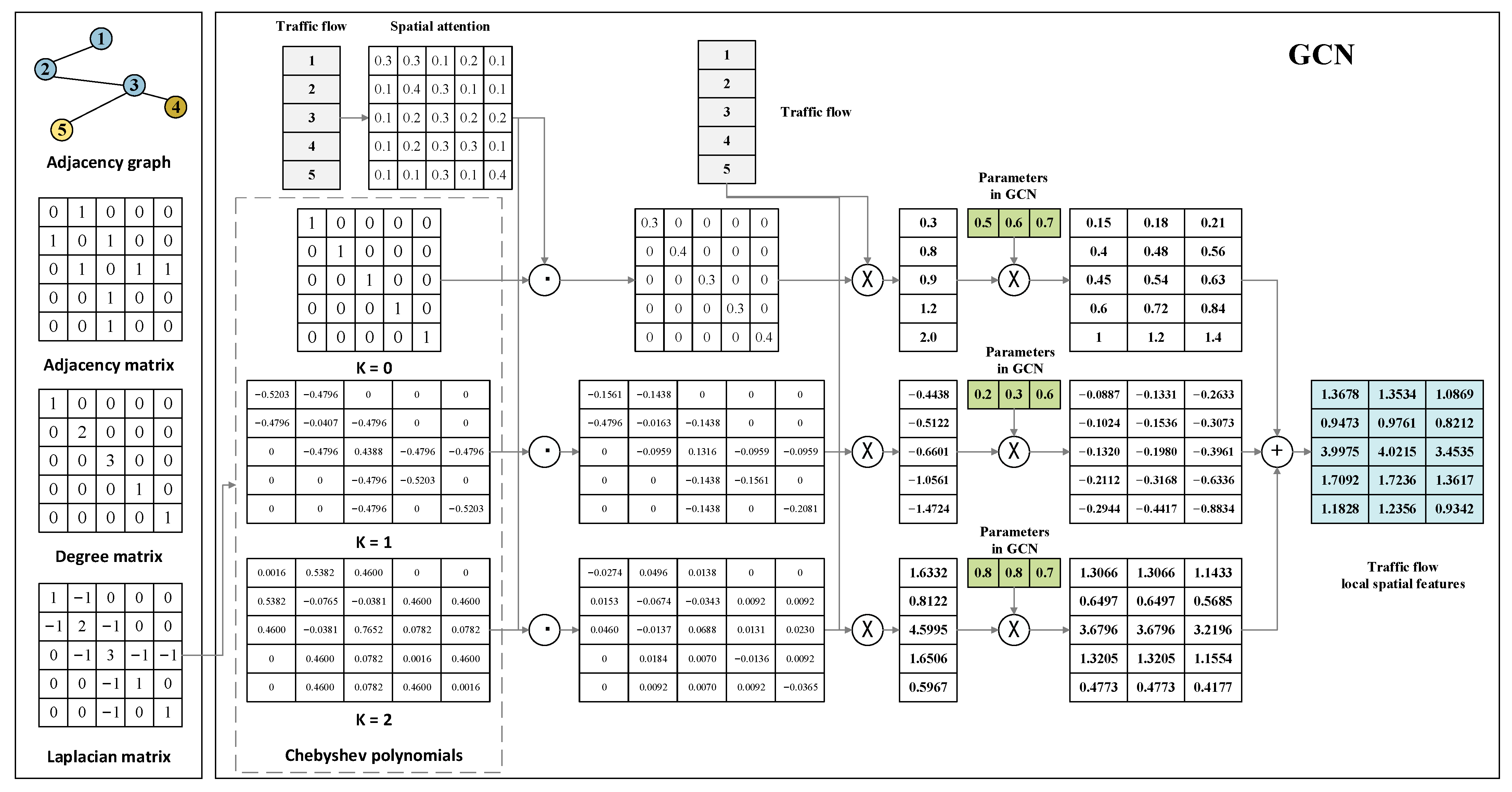
2.1. Traffic Network Modelling
2.2. Traffic Flow Forecasting
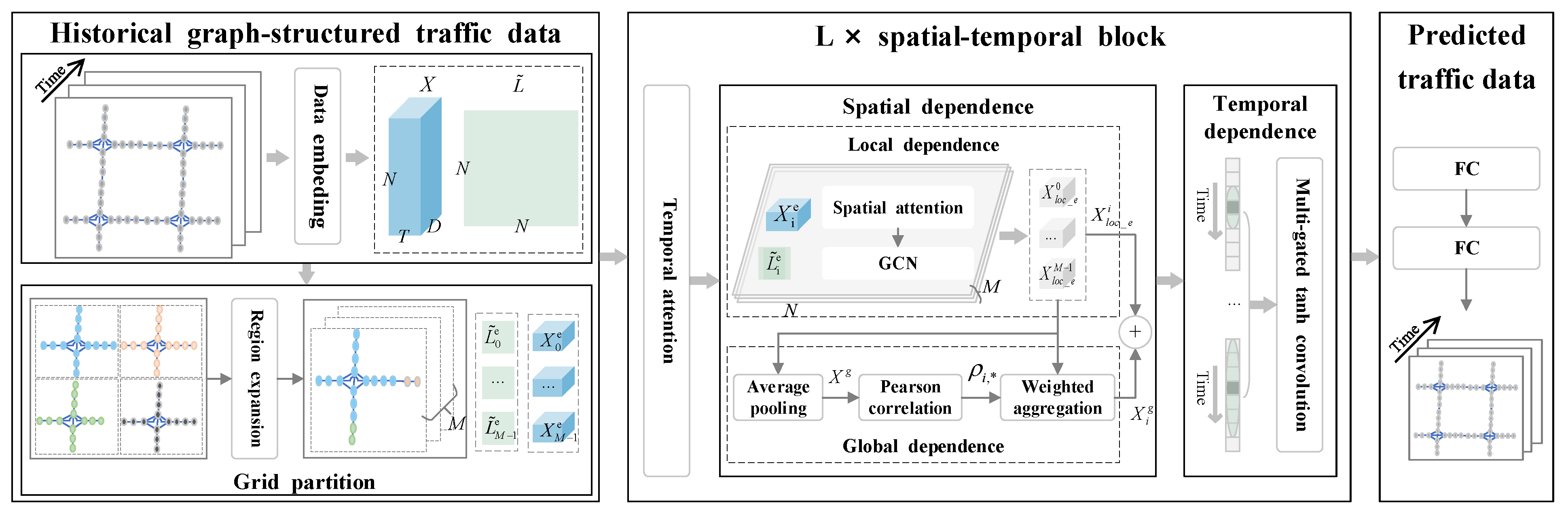
3. Proposed Forecasting Methodology
3.1. Subsection Data Embedding Module
3.2. Spatial–Temporal Feature Module
3.2.1. Dynamic Spatial–Temporal Attention Layer
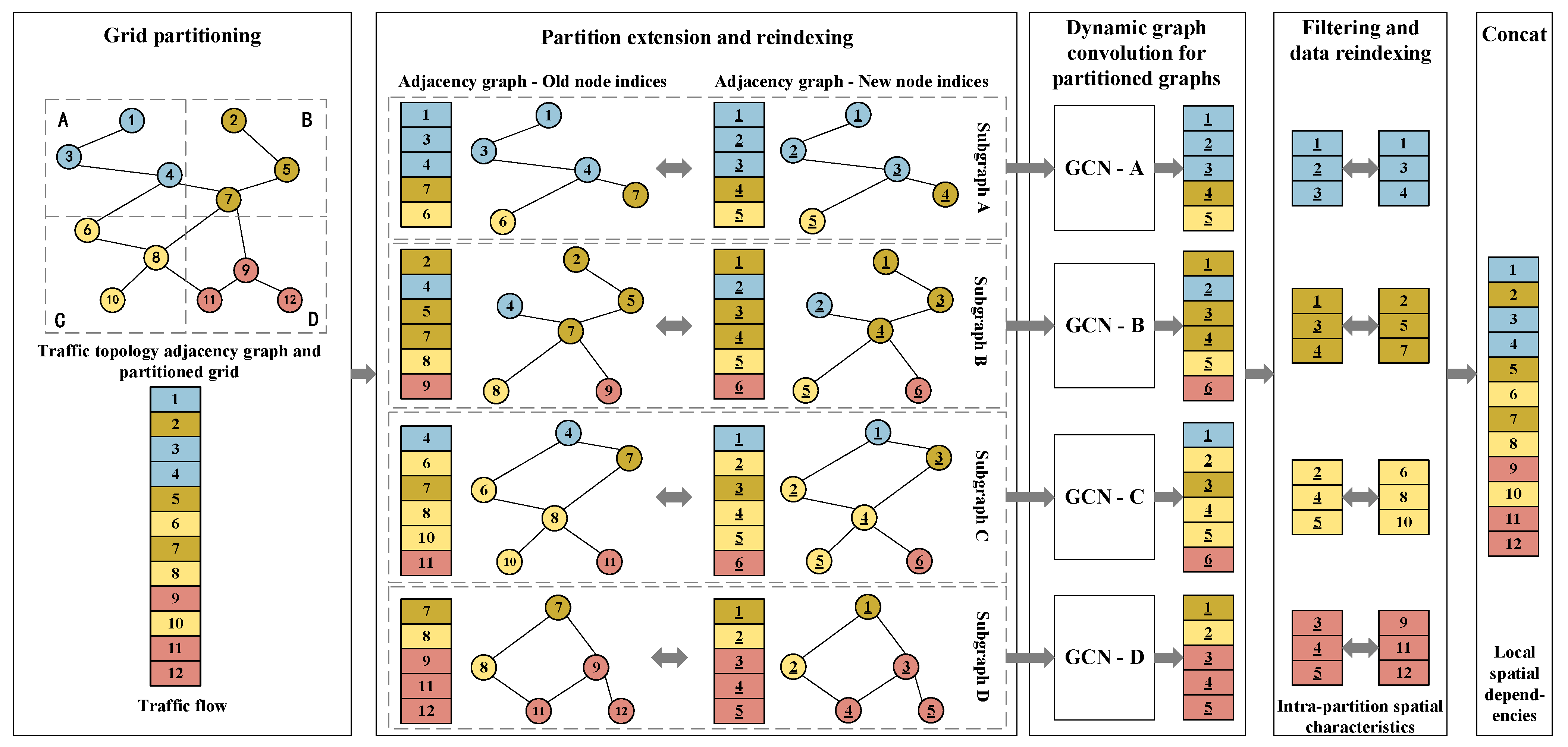
3.2.2. Spatial Dependency Layer
- 1.
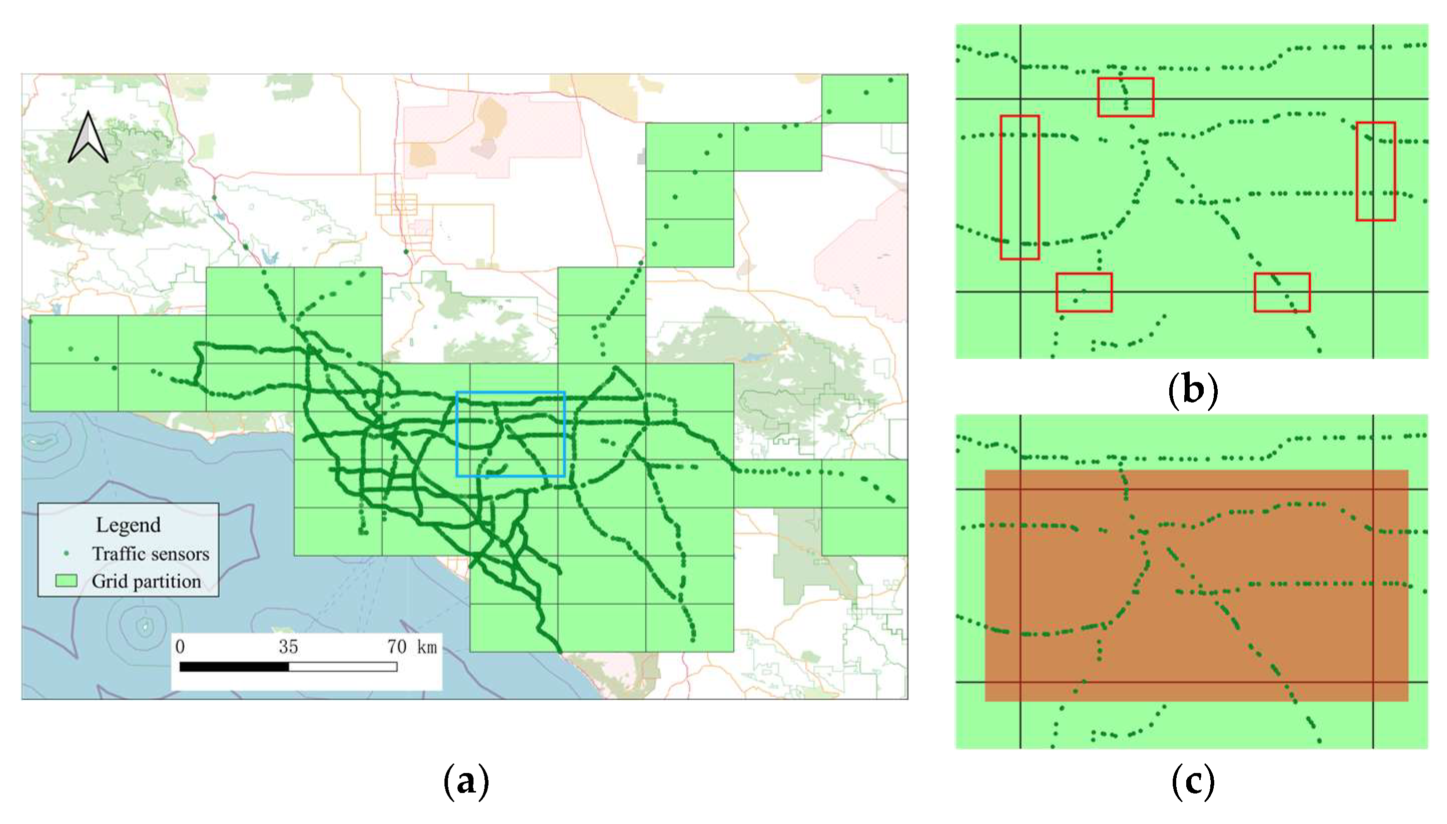
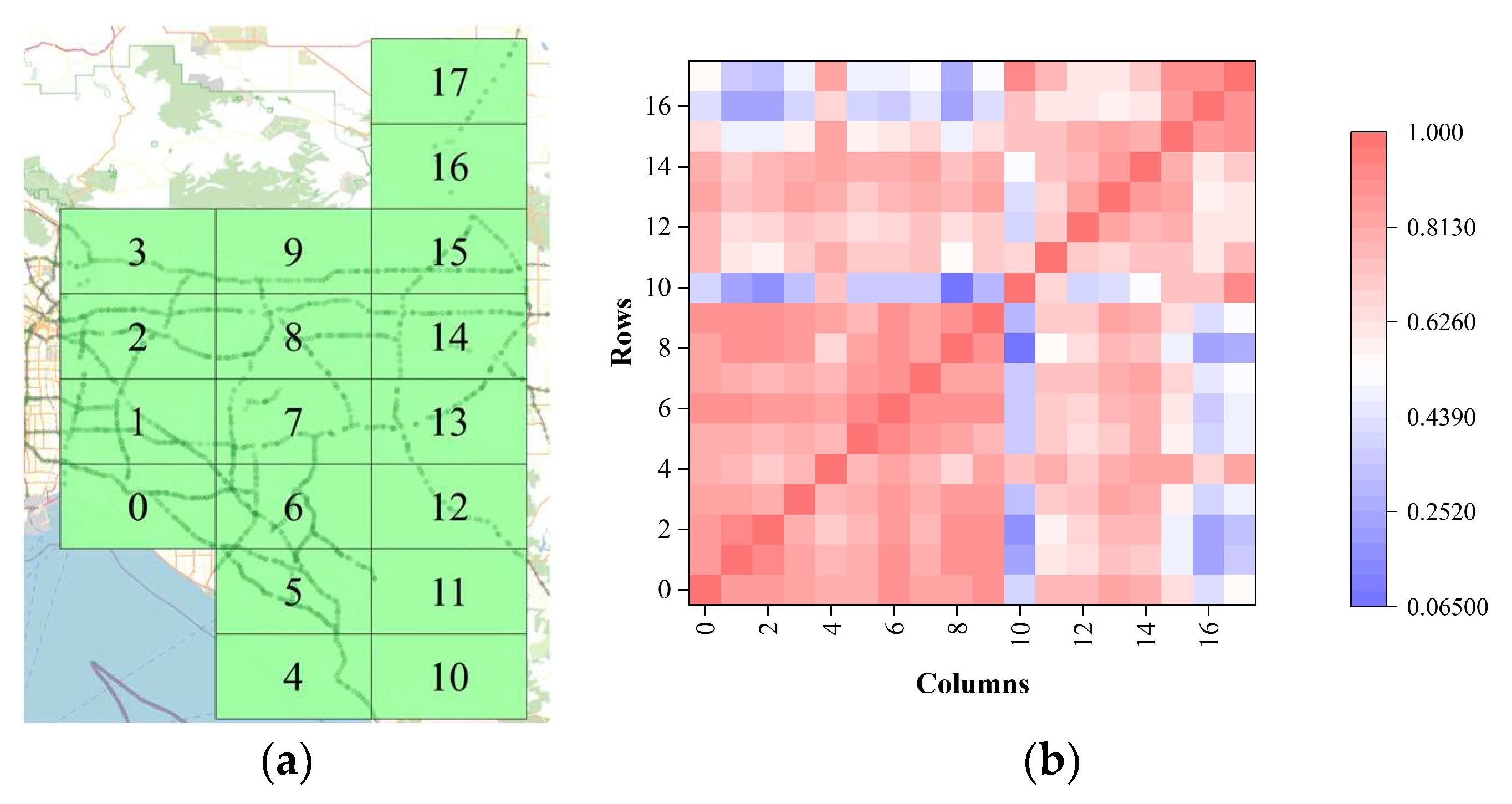
- Grid Partitioning
- 2.
- Identification of Local Spatial Dependencies
- 3.
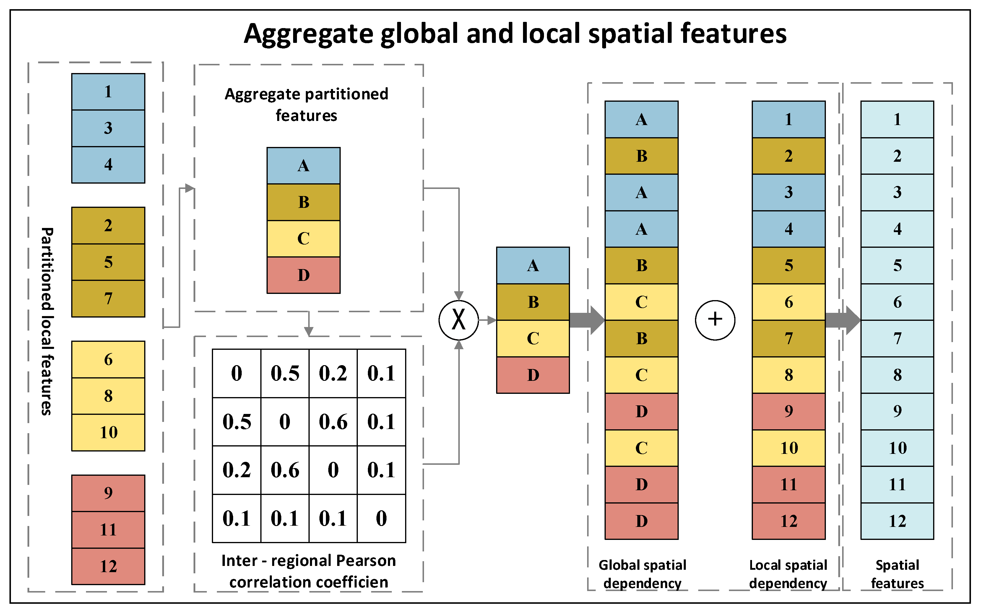
- Aggregation of Global Spatial Dependencies
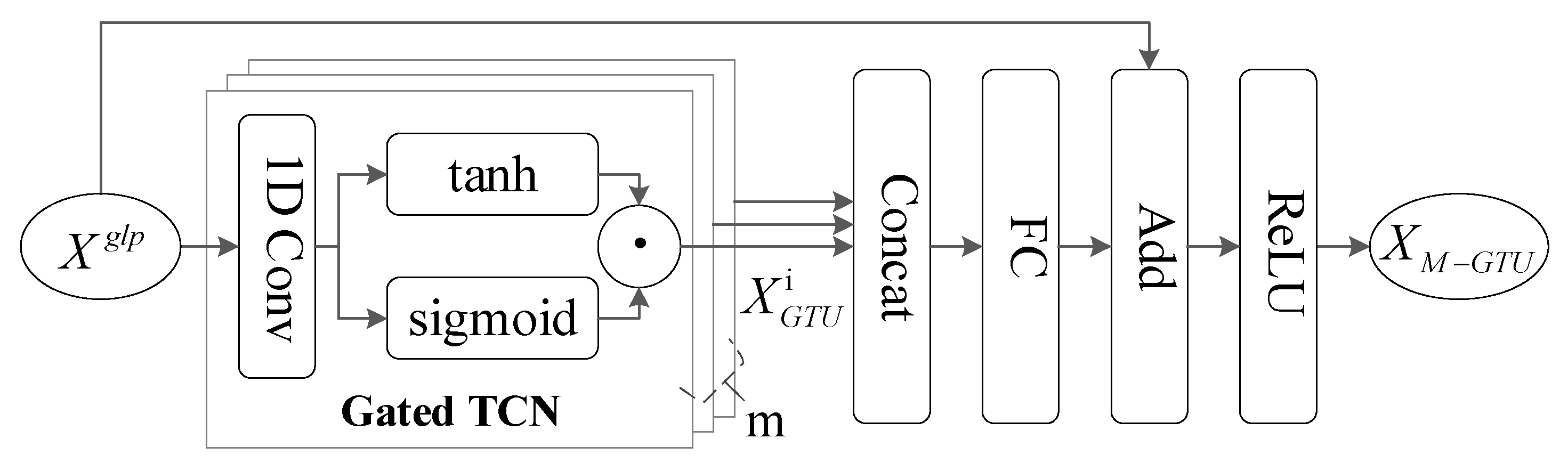
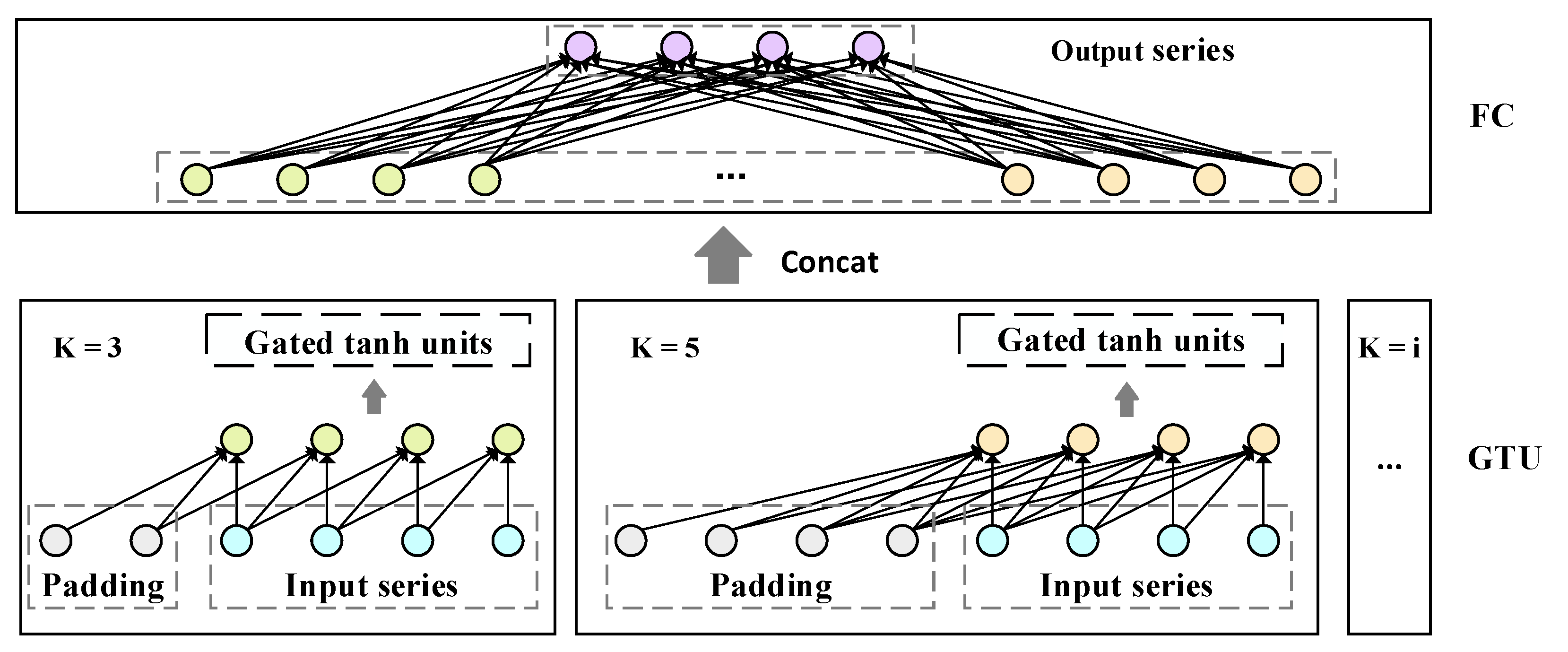
3.2.3. Temporal Dependency Layer
3.3. Prediction Module
4. Experimental Means and Methods
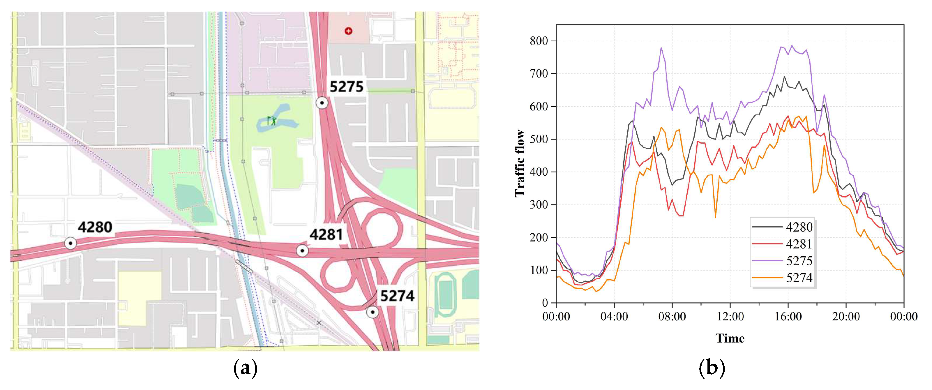
4.1. Datasets
4.2. Evaluated Models
- STGCN [14], which combines graph convolution with gated causal convolution to extract spatial–temporal features.
- DCRNN [31], which uses diffusion graph convolution to improve the GRU module, providing strong interpretability for dynamic spatial dependency and employs an encoder–decoder architecture to capture the spatial–temporal correlations in timeseries traffic data.
- GWNET [25], which utilises an adaptive adjacency matrix to represent adjacency relationships, combines a GCN with diffusion convolution to aggregate the transformed feature information from different neighbourhood orders, and captures temporal dependencies using gated dilated causal convolution.
- ASTGCN [17], which employs attention mechanisms to capture dynamic temporal and spatial correlations and combines the GCN and TCN to effectively capture dynamic spatial–temporal dependencies.
- AGCRN [23], which explores the parameters of spatial graph convolution using an adaptive adjacency matrix, learns a parameter space for each node, and integrates adaptive graph convolution into a GRU network to capture spatial–temporal dependencies.
- STGODE [19], which constructs a semantic similarity matrix using DTW and combines it with an original adjacency matrix, employs a continuous graph neural network to address GCN over-smoothing and capture dynamic spatial relationships, and uses a TCN to capture temporal dependencies.
- STWave [32], which employs a novel disentangled fusion framework that decomposes complex traffic data into stable trends and fluctuating events and introduces a new query sampling strategy and graph wavelet-based positional encoding to capture dynamic spatial dependencies effectively.
- HGCN [33] applies spectral clustering to aggregate node-level information at the region level and uses spatial gated convolution to capture hierarchical features. A region-to-node information transfer module facilitates cross-level fusion, and both node- and region-level features are jointly used for traffic prediction.
- HSTGODE [34], which builds on a hierarchical modelling framework similar to HGCN, introduces a spatiotemporal ODE module for continuous hierarchical representation learning. It also adopts attention mechanisms and skip connections to facilitate iterative and effective cross-level feature fusion.
- RemEmb, in which the day and week data embedding was removed.
- RemExt, in which the region expansion module was removed, leading to incomplete adjacency relationships for the sensors at the partition edges.
- RemPart, in which the partitioning was removed and a dynamic GCN was applied to the entire traffic graph.
- RemGlo, in which the global dependency module was removed, leaving only the local spatial dependencies.
- GPMK-M, in which the grid partitioning method was replaced with K-means clustering based on the spatial location.
- RemMGTU, in which the multi-scale gated temporal convolution module was replaced with a single-layer TCN.
4.3. Experiment Settings
5. Experiment Results and Discussion
5.1. Predictive Accuracy
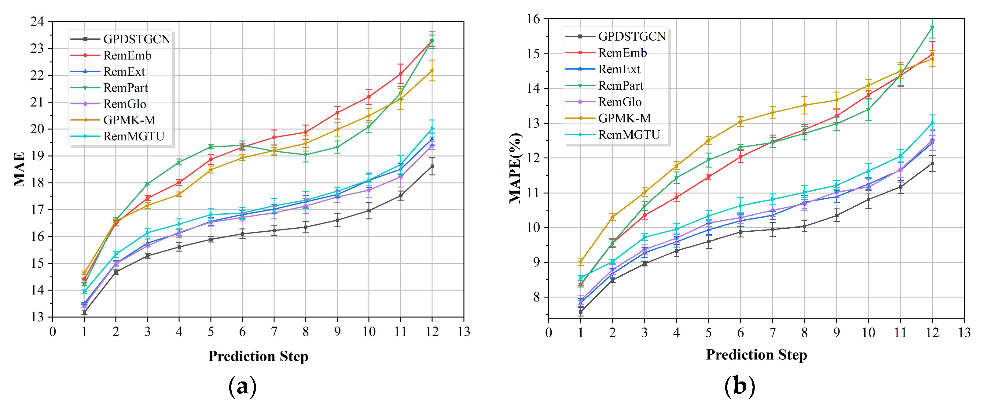
5.2. Ablation Study
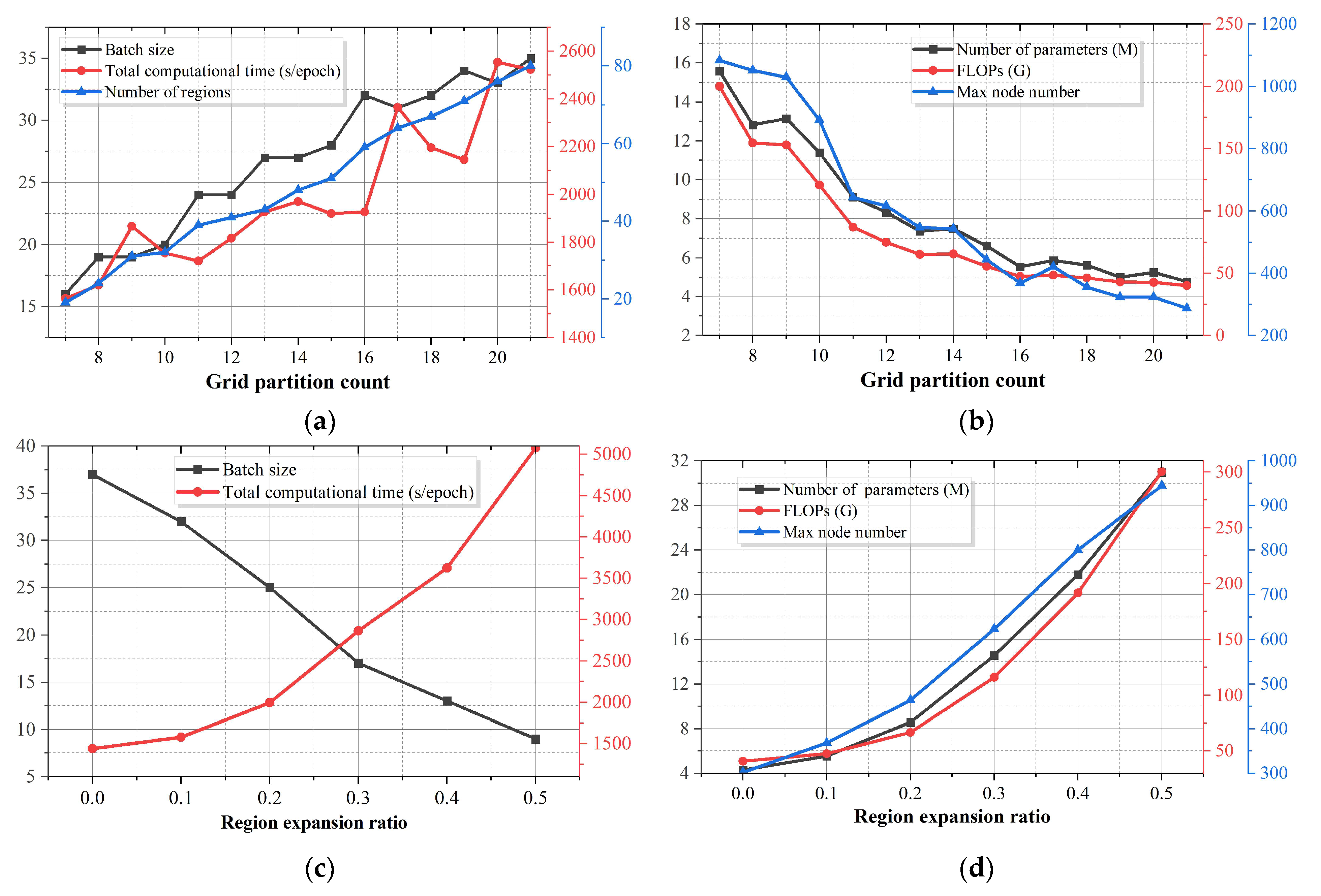
5.3. Efficiency
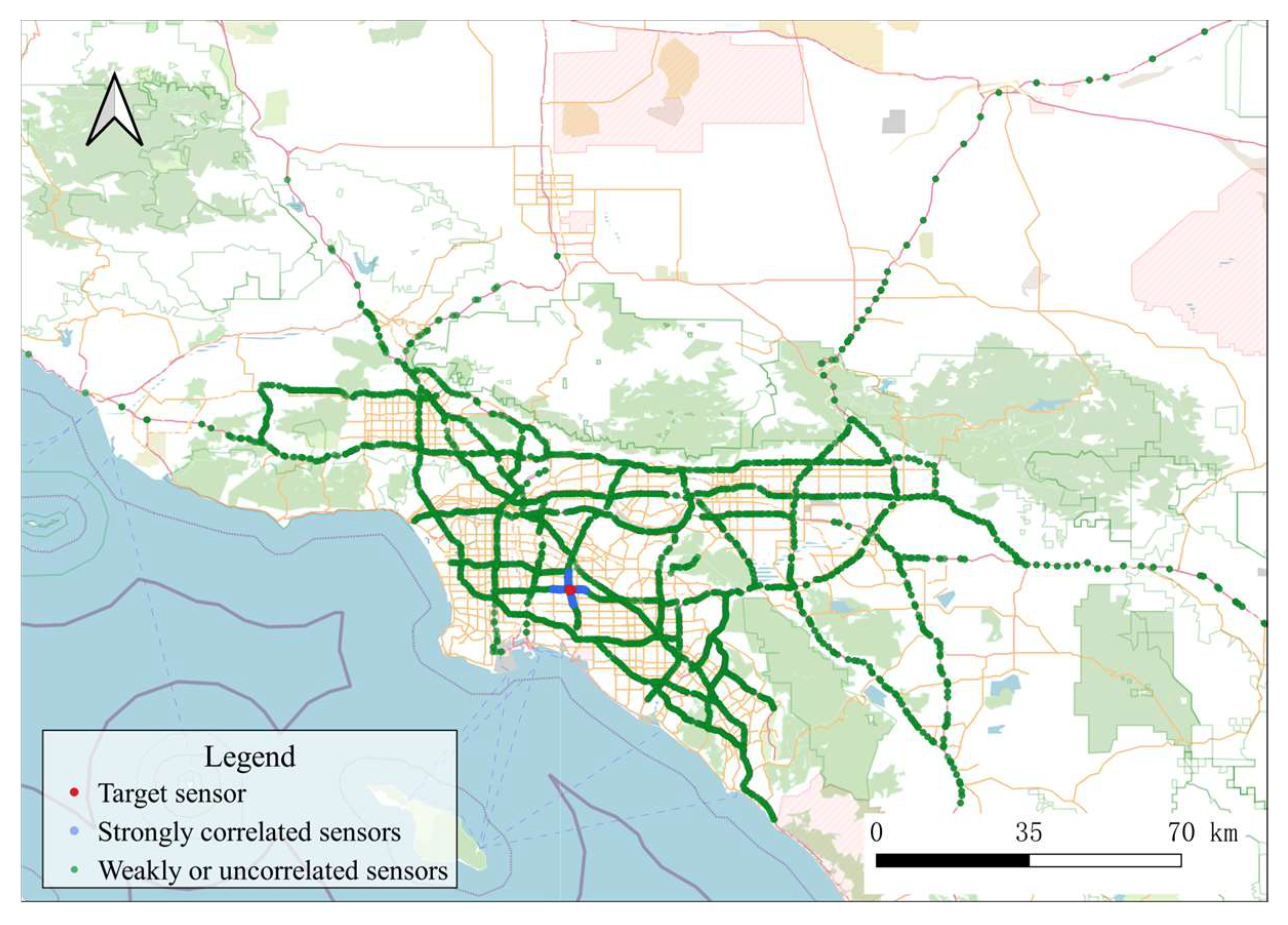
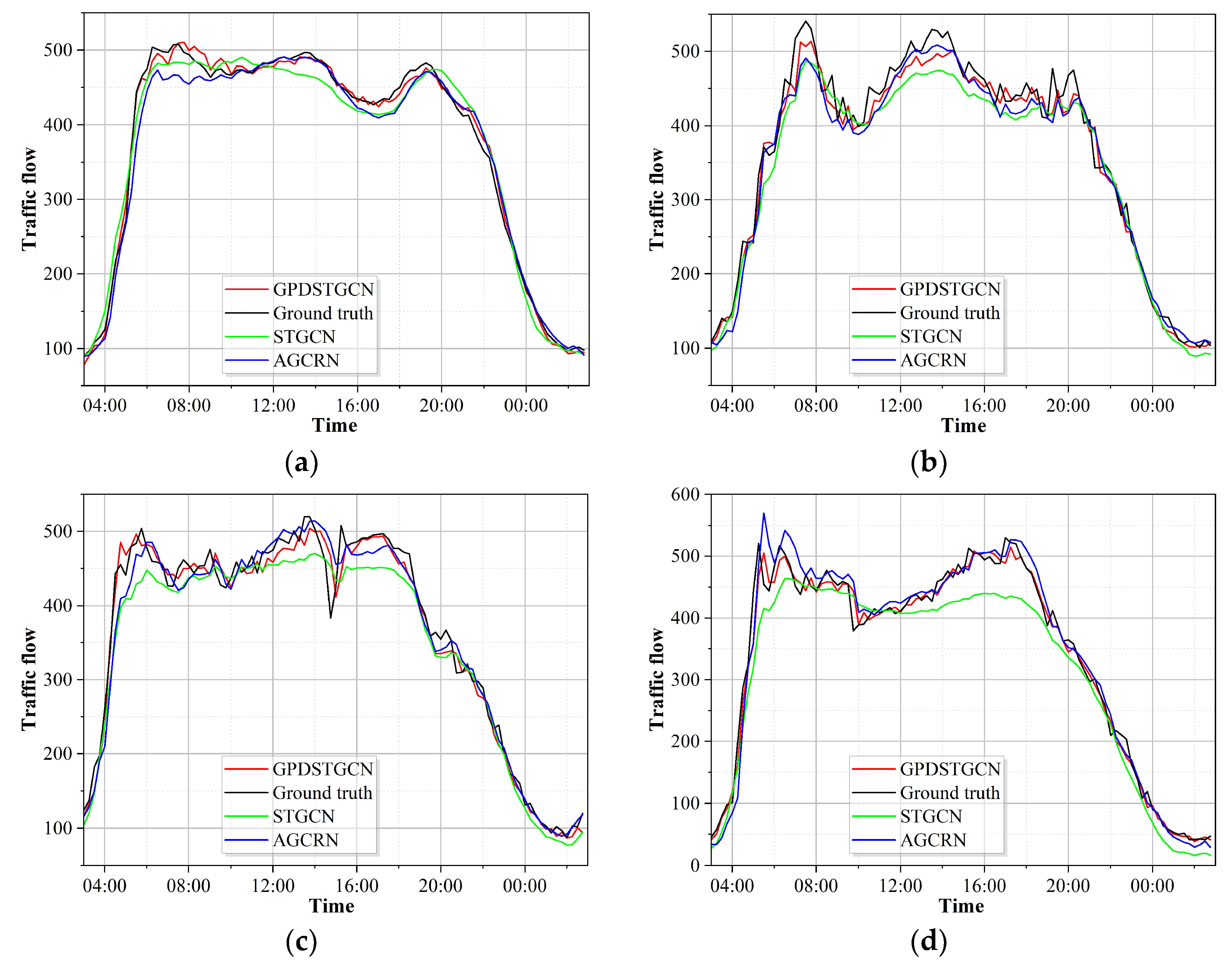
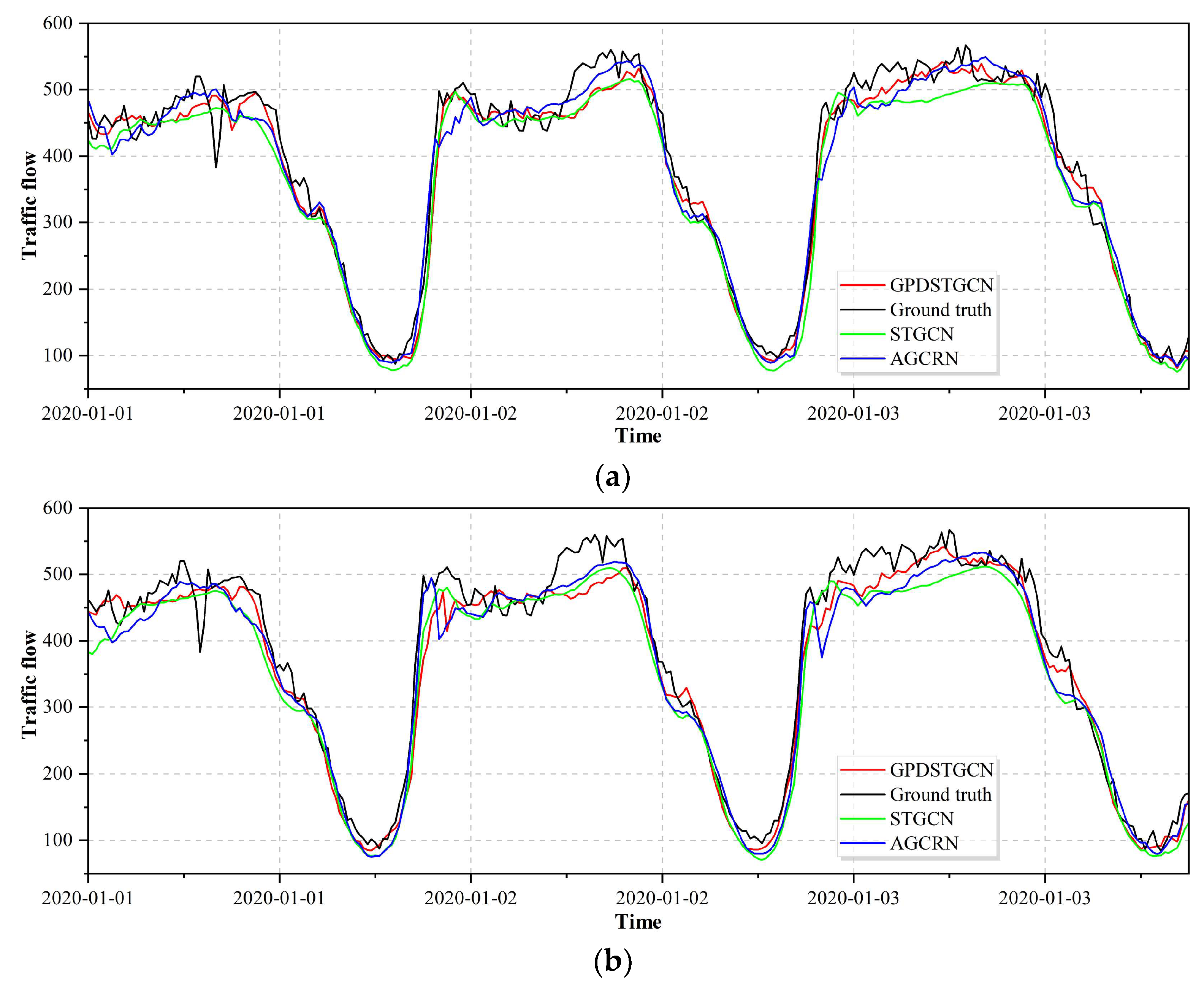
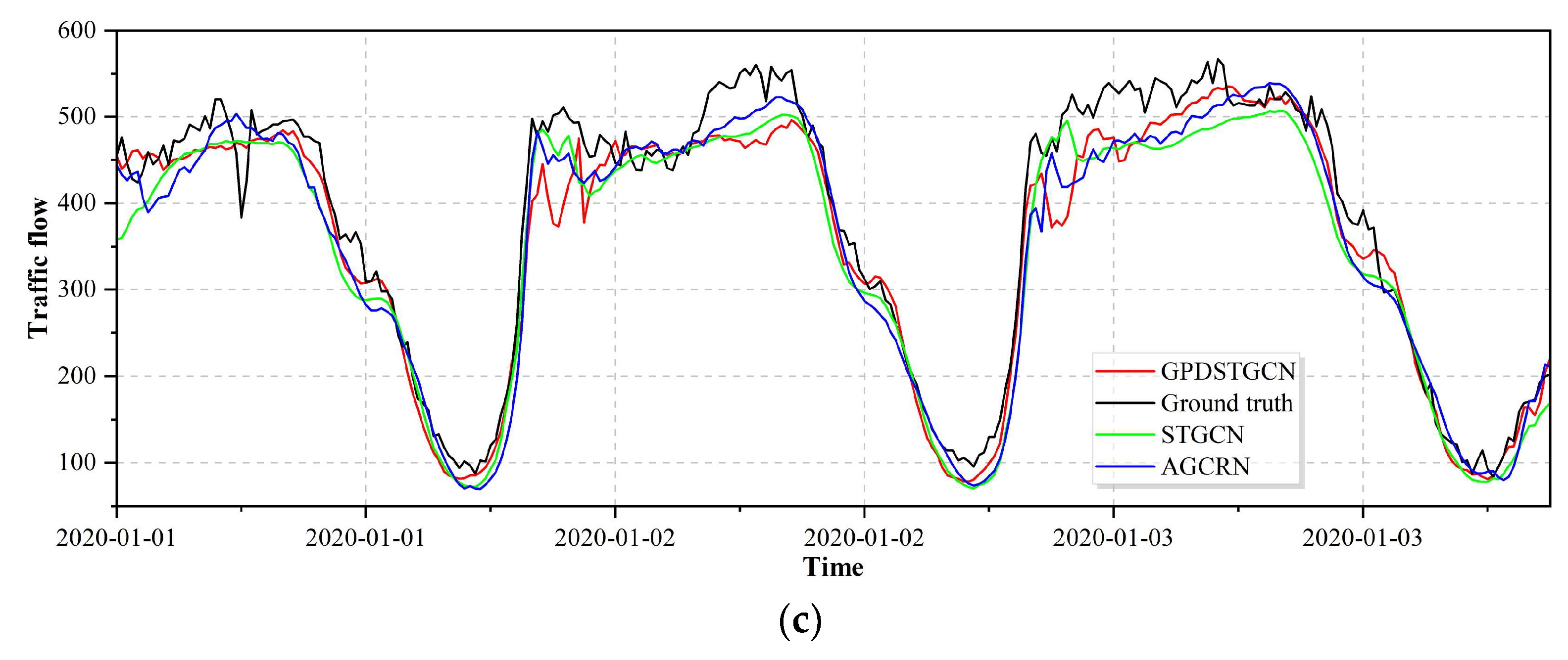
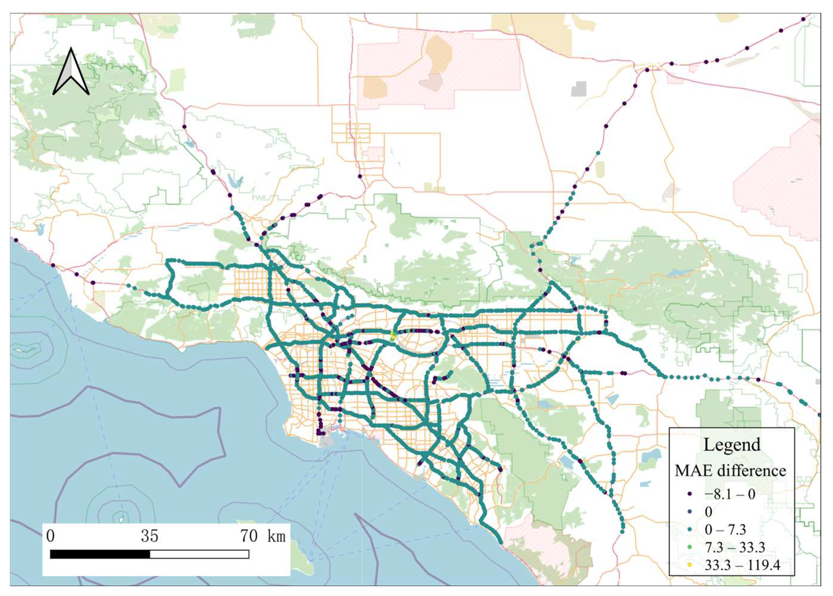
5.4. Visualisation
6. Conclusions
Author Contributions
Funding
Data Availability Statement
Conflicts of Interest
Appendix A
References
- Zhao, D.; Dai, Y.; Zhang, Z. Computational intelligence in urban traffic signal control: A survey. IEEE Trans. Syst. Man Cybern. Part C (Appl. Rev.) 2011, 42, 485–494. [Google Scholar] [CrossRef]
- Zhang, J.; Wang, F.-Y.; Wang, K.; Lin, W.-H.; Xu, X.; Chen, C. Data-driven intelligent transportation systems: A survey. IEEE Trans. Intell. Transp. Syst. 2011, 12, 1624–1639. [Google Scholar] [CrossRef]
- Yin, X.; Wu, G.; Wei, J.; Shen, Y.; Qi, H.; Yin, B. Deep learning on traffic prediction: Methods, analysis, and future directions. IEEE Trans. Intell. Transp. Syst. 2021, 23, 4927–4943. [Google Scholar] [CrossRef]
- Duan, Y.; Chen, N.; Shen, S.; Zhang, P.; Qu, Y.; Yu, S. FDSA-STG: Fully dynamic self-attention spatio-temporal graph networks for intelligent traffic flow prediction. IEEE Trans. Veh. Technol. 2022, 71, 9250–9260. [Google Scholar] [CrossRef]
- Ma, C.; Dai, G.; Zhou, J. Short-term traffic flow prediction for urban road sections based on time series analysis and LSTM_BILSTM method. IEEE Trans. Intell. Transp. Syst. 2021, 23, 5615–5624. [Google Scholar] [CrossRef]
- Williams, B.M.; Hoel, L.A. Modeling and forecasting vehicular traffic flow as a seasonal ARIMA process: Theoretical basis and empirical results. J. Transp. Eng. 2003, 129, 664–672. [Google Scholar] [CrossRef]
- Liu, J.; Guan, W. A summary of traffic flow forecasting methods. J. Highw. Transp. Res. Dev. 2004, 21, 82–85. [Google Scholar]
- Lingras, P.; Sharma, S.; Zhong, M. Prediction of recreational travel using genetically designed regression and time-delay neural network models. Transp. Res. Rec. 2002, 1805, 16–24. [Google Scholar] [CrossRef]
- Ma, X.; Tao, Z.; Wang, Y.; Yu, H.; Wang, Y. Long short-term memory neural network for traffic speed prediction using remote microwave sensor data. Transp. Res. Part C Emerg. Technol. 2015, 54, 187–197. [Google Scholar] [CrossRef]
- Yao, H.; Tang, X.; Wei, H.; Zheng, G.; Li, Z. Revisiting spatial-temporal similarity: A deep learning framework for traffic prediction. In Proceedings of the AAAI Conference on Artificial Intelligence, Honolulu, HI, USA, 27 January–1 February 2019; pp. 5668–5675. [Google Scholar]
- Guo, K.; Hu, Y.; Qian, Z.; Sun, Y.; Gao, J.; Yin, B. Dynamic graph convolution network for traffic forecasting based on latent network of Laplace matrix estimation. IEEE Trans. Intell. Transp. Syst. 2020, 23, 1009–1018. [Google Scholar] [CrossRef]
- Zhang, J.; Chen, F.; Cui, Z.; Guo, Y.; Zhu, Y. Deep learning architecture for short-term passenger flow forecasting in urban rail transit. IEEE Trans. Intell. Transp. Syst. 2020, 22, 7004–7014. [Google Scholar] [CrossRef]
- Geng, X.; Li, Y.; Wang, L.; Zhang, L.; Yang, Q.; Ye, J.; Liu, Y. Spatiotemporal multi-graph convolution network for ride-hailing demand forecasting. In Proceedings of the AAAI Conference on Artificial Intelligence, Honolulu, HI, USA, 27 January–1 February 2019; pp. 3656–3663. [Google Scholar]
- Yu, B.; Yin, H.; Zhu, Z. Spatio-temporal graph convolutional networks: A deep learning framework for traffic forecasting. arXiv 2017, arXiv:1709.04875. [Google Scholar]
- Tedjopurnomo, D.A.; Bao, Z.; Zheng, B.; Choudhury, F.M.; Qin, A.K. A survey on modern deep neural network for traffic prediction: Trends, methods and challenges. IEEE Trans. Knowl. Data Eng. 2020, 34, 1544–1561. [Google Scholar] [CrossRef]
- Yao, H.; Tang, X.; Wei, H.; Zheng, G.; Yu, Y.; Li, Z. Modeling spatial-temporal dynamics for traffic prediction. arXiv 2018, arXiv:1803.01254. [Google Scholar]
- Guo, S.; Lin, Y.; Feng, N.; Song, C.; Wan, H. Attention based spatial-temporal graph convolutional networks for traffic flow forecasting. In Proceedings of the AAAI Conference on Artificial Intelligence, Honolulu, HI, USA, 27 January–1 February 2019; pp. 922–929. [Google Scholar]
- Lan, S.; Ma, Y.; Huang, W.; Wang, W.; Yang, H.; Li, P. Dstagnn: Dynamic spatial-temporal aware graph neural network for traffic flow forecasting. In Proceedings of the International Conference on Machine Learning, Baltimore, MD, USA, 17–23 July 2022; pp. 11906–11917. [Google Scholar]
- Fang, Z.; Long, Q.; Song, G.; Xie, K. Spatial-temporal graph ode networks for traffic flow forecasting. In Proceedings of the 27th ACM SIGKDD Conference on Knowledge Discovery & Data Mining, Virtual Event, 14–18 August 2021; pp. 364–373. [Google Scholar]
- Jiang, J.; Han, C.; Zhao, W.X.; Wang, J. Pdformer: Propagation delay-aware dynamic long-range transformer for traffic flow prediction. In Proceedings of the AAAI Conference on Artificial Intelligence, Washington, DC, USA, 7–14 February 2023; pp. 4365–4373. [Google Scholar]
- Zheng, C.; Fan, X.; Wang, C.; Qi, J. Gman: A graph multi-attention network for traffic prediction. In Proceedings of the AAAI Conference on Artificial Intelligence, New York, NY, USA, 7–12 February 2020; pp. 1234–1241. [Google Scholar]
- Li, F.; Feng, J.; Yan, H.; Jin, G.; Yang, F.; Sun, F.; Jin, D.; Li, Y. Dynamic graph convolutional recurrent network for traffic prediction: Benchmark and solution. ACM Trans. Knowl. Discov. Data 2023, 17, 1–21. [Google Scholar] [CrossRef]
- Bai, L.; Yao, L.; Li, C.; Wang, X.; Wang, C. Adaptive graph convolutional recurrent network for traffic forecasting. Adv. Neural Inf. Process. Syst. 2020, 33, 17804–17815. [Google Scholar]
- Shao, Z.; Zhang, Z.; Wei, W.; Wang, F.; Xu, Y.; Cao, X.; Jensen, C.S. Decoupled dynamic spatial-temporal graph neural network for traffic forecasting. arXiv 2022, arXiv:2206.09112. [Google Scholar] [CrossRef]
- Wu, Z.; Pan, S.; Long, G.; Jiang, J.; Zhang, C. Graph wavenet for deep spatial-temporal graph modeling. arXiv 2019, arXiv:1906.00121. [Google Scholar]
- Liu, X.; Xia, Y.; Liang, Y.; Hu, J.; Wang, Y.; Bai, L.; Huang, C.; Liu, Z.; Hooi, B.; Zimmermann, R. Largest: A benchmark dataset for large-scale traffic forecasting. Adv. Neural Inf. Process. Syst. 2024, 36, 75354–75371. [Google Scholar]
- Zhang, Y.; Li, Y.; Zhang, F. Multi-level urban street representation with street-view imagery and hybrid semantic graph. ISPRS J. Photogramm. Remote Sens. 2024, 218, 19–32. [Google Scholar] [CrossRef]
- Feng, X.; Guo, J.; Qin, B.; Liu, T.; Liu, Y. Effective Deep Memory Networks for Distant Supervised Relation Extraction. In Proceedings of the Twenty-Sixth International Joint Conference on Artificial Intelligence (IJCAI-17), Melbourne, Australia, 19–25 August 2017; pp. 1–7. [Google Scholar]
- Zhang, T.; Wang, J.; Liu, J. A gated generative adversarial imputation approach for signalized road networks. IEEE Trans. Intell. Transp. Syst. 2021, 23, 12144–12160. [Google Scholar] [CrossRef]
- Defferrard, M.; Bresson, X.; Vandergheynst, P. Convolutional neural networks on graphs with fast localized spectral filtering. Adv. Neural Inf. Process. Syst. 2016, 29, 3844–3852. [Google Scholar]
- Li, Y.; Yu, R.; Shahabi, C.; Liu, Y. Diffusion convolutional recurrent neural network: Data-driven traffic forecasting. arXiv 2017, arXiv:1707.01926. [Google Scholar]
- Fang, Y.; Qin, Y.; Luo, H.; Zhao, F.; Xu, B.; Zeng, L.; Wang, C. When spatio-temporal meet wavelets: Disentangled traffic forecasting via efficient spectral graph attention networks. In Proceedings of the 2023 IEEE 39th International Conference on Data Engineering (ICDE), Anaheim, CA, USA, 3–7 April 2023; pp. 517–529. [Google Scholar]
- Guo, K.; Hu, Y.; Sun, Y.; Qian, S.; Gao, J.; Yin, B. Hierarchical graph convolution network for traffic forecasting. In Proceedings of the AAAI Conference on Artificial Intelligence, Virtul, 19–21 May 2021; pp. 151–159. [Google Scholar]
- Xu, T.; Deng, J.; Ma, R.; Zhang, Z.; Zhao, Y.; Zhao, Z.; Zhang, J. Hierarchical spatio-temporal graph ODE networks for traffic forecasting. Inf. Fusion 2025, 113, 102614. [Google Scholar] [CrossRef]


| Data | Model | Horizon3 | Horizon6 | Horizon12 | Average | ||||||||
|---|---|---|---|---|---|---|---|---|---|---|---|---|---|
| MAE | RMSE | MAPE | MAE | RMSE | MAPE | MAE | RMSE | MAPE | MAE | RMSE | MAPE | ||
| GLA | STGCN | 16.22 | 25.67 | 10.64% | 17.61 | 28.20 | 11.38% | 19.74 | 31.96 | 11.99% | 17.53 | 28.05 | 11.21% |
| GWNET | 16.66 | 26.85 | 9.57% | 19.51 | 31.01 | 11.66% | 23.85 | 37.27 | 14.58% | 19.43 | 30.85 | 11.63% | |
| DCRNN | 19.42 | 30.51 | 11.3% | 22.48 | 34.86 | 13.53% | 27.70 | 42.61 | 17.48% | 22.42 | 34.88 | 13.61% | |
| AGCRN | 15.72 | 25.64 | 9.33% | 17.53 | 28.60 | 10.81% | 19.93 | 32.42 | 11.89% | 17.33 | 28.24 | 10.44% | |
| ASTGCN | 22.69 | 37.00 | 13.17% | 32.32 | 51.10 | 19.97% | 45.60 | 69.72 | 31.59% | 32.35 | 50.84 | 20.67% | |
| STGODE | 16.76 | 26.83 | 9.95% | 18.82 | 30.14 | 11.63% | 21.69 | 34.85 | 14.37% | 18.58 | 29.81 | 11.59% | |
| STWave | 19.24 | 31.54 | 10.49% | 26.04 | 42.13 | 14.64% | 36.80 | 58.42 | 21.93% | 26.40 | 42.54 | 15.14% | |
| HGCN | 17.04 | 26.91 | 10.61% | 20.19 | 31.39 | 13.03% | 24.63 | 37.43 | 12.99% | 20.08 | 31.12 | 12.99% | |
| HSTGODE | 16.88 | 27.21 | 9.88% | 19.07 | 30.47 | 11.78% | 23.05 | 36.25 | 14.89% | 19.14 | 36.25 | 14.89% | |
| MY | 15.29 | 25.17 | 8.97% | 16.14 | 26.73 | 9.82% | 18.52 | 30.15 | 11.77% | 16.09 | 26.56 | 9.82% | |
| CA | STGCN | 15.50 | 25.18 | 11.41% | 16.64 | 27.33 | 12.16% | 18.27 | 30.17 | 13.53% | 16.50 | 27.07 | 12.10% |
| GWNET | 16.48 | 26.93 | 12.81% | 19.22 | 30.83 | 15.93% | 23.41 | 36.70 | 20.69% | 19.17 | 30.64 | 15.98% | |
| DCRNN | 21.48 | 34.36 | 15.95% | 28.69 | 45.46 | 21.36% | 39.06 | 60.20 | 31.93% | 28.84 | 45.38 | 22.31% | |
| STGODE | 16.05 | 26.08 | 11.85% | 17.81 | 29.00 | 13.84% | 20.41 | 33.31 | 16.97% | 17.67 | 28.79 | 13.76% | |
| STWave | 19.22 | 31.67 | 12.84% | 26.34 | 42.67 | 18.67% | 37.18 | 58.99 | 28.71% | 26.55 | 42.88 | 19.28% | |
| HGCN | 16.49 | 26.74 | 11.86% | 19.19 | 30.63 | 14.64% | 22.74 | 35.74 | 18.37% | 18.97 | 30.25 | 14.51% | |
| MY | 14.51 | 24.31 | 10.55% | 15.23 | 25.64 | 11.53% | 17.31 | 28.69 | 13.36% | 15.25 | 25.56 | 11.61% | |
| Step (Hours) | Our | STGCN | AGCRN | STGODE | |||
|---|---|---|---|---|---|---|---|
| MAE | MAE | p-Value | MAE | p-Value | MAE | p-Value | |
| 1 | 15.61 | 16.70 | 5.1 × 10⁻⁶ | 16.33 | 1.7 × 10⁻⁴ | 17.34 | 2.0 × 10⁻⁶ |
| 2 | 16.40 | 18.09 | 2.2 × 10⁻⁶ | 18.22 | 1.1 × 10⁻⁶ | 19.55 | 2.1 × 10⁻⁵ |
| 2.25 | 16.70 | 18.52 | 5.5 × 10⁻⁶ | 18.68 | 1.2 × 10⁻⁶ | 20.12 | 3.4 × 10⁻⁵ |
| 2.5 | 17.00 | 18.86 | 1.1 × 10⁻⁵ | 18.99 | 3.1 × 10⁻⁶ | 20.57 | 4.4 × 10⁻⁵ |
| 2.75 | 17.52 | 19.17 | 9.8 × 10⁻⁵ | 19.33 | 7.7 × 10⁻⁶ | 20.98 | 9.7 × 10⁻⁵ |
| 3 | 18.52 | 19.73 | 0.0018 | 19.93 | 1.1 × 10⁻⁴ | 21.69 | 2.6 × 10⁻⁴ |
| Model | Functional Categories | Number of Lanes | |||||
|---|---|---|---|---|---|---|---|
| Interstate | US Highways | State Highways | Small | Medium | Large | Extra-Large | |
| GPDSTGCN | 16.47 | 21.19 | 14.66 | 6.63 | 15.29 | 22.15 | 20.14 |
| RemGlo | 17.14 | 21.98 | 15.22 | 6.94 | 15.87 | 23.35 | 21.24 |
| STGCN | 18.02 | 22.89 | 15.94 | 7.20 | 16.68 | 24.21 | 22.13 |
| AGCRN | 17.83 | 22.43 | 15.76 | 6.85 | 16.47 | 24.10 | 21.90 |
| STGODE | 18.98 | 24.37 | 17.06 | 7.42 | 17.64 | 25.84 | 23.41 |
| Model | GLA Dataset | CA Dataset | ||||||||
|---|---|---|---|---|---|---|---|---|---|---|
| BS | Train (s) | Infer (s) | Param | FLOPs | BS | Train (s) | Infer (s) | Param | FLOPs | |
| STGCN | 64 | 283 | 80 | 2.1 M | 163 M | 40 | 810 | 220 | 4.54 M | 366 M |
| GWNET | 20 | 2215 | 380 | 373.52 K | 5 G | 8 | 7558 | 1018 | 468.84 K | 11 G |
| AGCRN | 42 | 515 | 119 | 230.74 K | 9 G | -- | -- | -- | 278.40 K | 43 G |
| ASTGCN | 8 | 1950 | 243 | 59.12 M | 4220 G | -- | -- | -- | 296.48 M | 47,312 G |
| STGODE | 15 | 905 | 135 | 841.48 K | 6 G | 7 | 2520 | 381 | 1.01 M | 14 G |
| STWave | 11 | 1664 | 210 | 882.57 K | 44 G | 4 | 3794 | 502 | 882.58 K | 98 G |
| HGCN | 64 | 177 | 36 | 16.12 M | 61 G | 40 | 655 | 126 | 77.92 M | 646.18 G |
| HSTGODE | 12 | 4244 | 909 | 1.73 M | 3624 G | -- | -- | -- | 4.14 M | 40,750 G |
| RemPart | 5 | 6101 | 1292 | 59.66 M | 2894 G | -- | -- | -- | 297.33 M | 32,164 G |
| MY | 32 | 1763 | 163 | 4.29 M | 40 G | 16 | 7437 | 885 | 8.66 M | 149 G |
Disclaimer/Publisher’s Note: The statements, opinions and data contained in all publications are solely those of the individual author(s) and contributor(s) and not of MDPI and/or the editor(s). MDPI and/or the editor(s) disclaim responsibility for any injury to people or property resulting from any ideas, methods, instructions or products referred to in the content. |
© 2025 by the authors. Published by MDPI on behalf of the International Society for Photogrammetry and Remote Sensing. Licensee MDPI, Basel, Switzerland. This article is an open access article distributed under the terms and conditions of the Creative Commons Attribution (CC BY) license (https://creativecommons.org/licenses/by/4.0/).
Share and Cite
Gao, L.; Chen, L.; Qiu, A.; Wang, Q.; Wang, J.; Chen, C.; Zhang, F.; Ou’er, G. Grid Partition-Based Dynamic Spatial–Temporal Graph Convolutional Network for Large-Scale Traffic Flow Forecasting. ISPRS Int. J. Geo-Inf. 2025, 14, 207. https://doi.org/10.3390/ijgi14050207
Gao L, Chen L, Qiu A, Wang Q, Wang J, Chen C, Zhang F, Ou’er G. Grid Partition-Based Dynamic Spatial–Temporal Graph Convolutional Network for Large-Scale Traffic Flow Forecasting. ISPRS International Journal of Geo-Information. 2025; 14(5):207. https://doi.org/10.3390/ijgi14050207
Chicago/Turabian StyleGao, Lifeng, Liujia Chen, Agen Qiu, Qinglian Wang, Jianlong Wang, Cai Chen, Fuhao Zhang, and Geli Ou’er. 2025. "Grid Partition-Based Dynamic Spatial–Temporal Graph Convolutional Network for Large-Scale Traffic Flow Forecasting" ISPRS International Journal of Geo-Information 14, no. 5: 207. https://doi.org/10.3390/ijgi14050207
APA StyleGao, L., Chen, L., Qiu, A., Wang, Q., Wang, J., Chen, C., Zhang, F., & Ou’er, G. (2025). Grid Partition-Based Dynamic Spatial–Temporal Graph Convolutional Network for Large-Scale Traffic Flow Forecasting. ISPRS International Journal of Geo-Information, 14(5), 207. https://doi.org/10.3390/ijgi14050207