1. Introduction
Morphology, through the study of urban spatial forms, structures, and organizations, helps us understand how cities are laid out and developed [
1]. This is crucial for guiding practical activities such as urban planning, urban design, and urban management. The traditional paradigm for studying urban form involves the interpretation of figure–ground maps (also known as Nolli maps). These maps usually consist of only black and white, with black representing the figure and white representing the ground [
2]. In urban spaces, the figure typically refers to prominent, dominant spatial elements such as buildings and blocks, while the ground is the space surrounding the figure, like streets, squares, parks, and open spaces. The ground provides support and context for the figure, and the ground is generally more uniform, lacking the clear shapes and boundaries of the figure. Figure–ground maps offer the most detailed and accurate representation of how people experience and understand urban spaces [
3,
4].
The interpretation of Nolli maps often relies on morphometrics, which quantifies the spatial distribution, shape, size, and layout of urban elements through various algorithms. Researchers then understand the patterns contained in Nolli maps by seeking correlations or inherent patterns in the data [
5]. The morphometrics have gained significant momentum in the current urban research. However, statistical data often fail to fully describe the characteristics of a map. The tremendous success of deep learning in CV has inspired related researchers. In recent years, many researchers have used visual neural networks (primarily CNNs) to simulate human vision and interpret urban figure–ground maps [
6,
7,
8].
Using deep learning methods requires segmenting Nolli maps into smaller pieces as samples. A common approach is to cut the maps into grids. While this facilitates research, gridded samples often bisect building groups, resulting in fragmented morphologies [
9]. Additionally, to have as much “figure” as possible on the Nolli maps, densely built urban areas are most frequently used as datasets. This allows visual neural networks to learn effectively but neglects unique urban types located at the urban fringe and in towns. In this study, we utilized a vast and complex dataset to circumvent these issues. Our dataset includes tens of thousands of square kilometers of continuous land parcels, encompassing a wide variety of urban forms. We also divided samples according to the administrative boundaries of communities or villages, thus avoiding the morphological fragmentation caused by gridding.
It is challenging to conduct urban morphology discovery on such complex datasets because there are significant differences in the building density and scale of the samples, which can significantly interfere with the judgment of visual neural networks. However, we hope that visual neural networks can ignore these elements and focus on the morphological characteristics of building groups. To overcome these difficulties, we have designed a new image deformation pipeline for contrastive learning based on visual neural networks. The core of this pipeline involves performing restricted random cropping on images, which ensures that the newly cropped images always focus on a specific building group and include an appropriate number of buildings. When we deform an original sample multiple times simultaneously, we also ensure that these deformed samples focus on the same building group. This holds significant importance in contrastive learning, which is one of the most commonly used methods for morphological studies in deep learning.
In past research, there has been a deficiency: the use of visual neural networks has almost entirely followed the research paradigm from the field of computer vision, failing to effectively utilize the existing knowledge of morphology. To explore the integration of existing morphological knowledge with visual neural networks, we have designed a new loss function that incorporates morphometrics. Although this loss function simply considers the building area ratio for each sample, experiments have shown that this strategy successfully guides the parameter optimization process of visual neural networks with morphological indicators. Intuitively, this change allows the model to initially “recognize” the similarity between samples, without necessarily treating all augmented views from different samples as negative pairs.
To demonstrate the effectiveness of our method, we designed three SimCLR frameworks [
10], named SimCLR 1, 2, and 3, which, respectively, include: the original SimCLR framework, the SimCLR framework with our image deformation pipeline, and the SimCLR framework with both our image deformation pipeline and loss function. They are all followed by k-means for clustering. We then used three representative Chinese cities, Shanghai, Beijing, and Chongqing, as experimental materials for separate experiments. In each experiment, we considered the entire jurisdiction of the city (tens of thousands of square kilometers) and used Nolli maps containing only a single village-level administrative area as individual samples. Eventually, each pipeline categorized these samples into five classes. We submitted the classification results to professionals from the architecture school for evaluation. The evaluation results showed that SimCLR 1 failed to complete the task, while SimCLR 2 and 3 effectively completed the classification task. This proved the effectiveness of our image deformation pipeline. Additionally, we analyzed the variance of the building area ratio within the clusters, which demonstrated that our loss function successfully guided the classification tendency of the pipelines. Finally, taking Shanghai as an example, we analyzed the urban functions and historical development of the discovered urban types.
Compared to previous surveys, the contributions of our survey can be summarized as follows:
The comprehensive discovery and analysis of urban forms across three Chinese cities was completed. This not only identified urban types located in city centers but also included those at the urban fringe and in towns.
A new image deformation pipeline was designed to enable visual neural networks to focus on extracting the morphological characteristics of building groups.
The NT-Xent loss was refined to enable visual neural networks to learn knowledge about morphological indicators.
The remainder of this paper is organized as follows:
Section 2 reviews the related morphology studies and deep learning methods.
Section 3 provides the details of the methodology and study areas. The experimental results and analysis are presented in
Section 4. The paper ends with a discussion in
Section 5 and conclusion in
Section 6.
2. Related Work
Identifying urban morphological types is an important way for researchers to understand urban construction, as specific urban morphological types are often associated with particular cultural connotations and geographical forms. The process of using computers to identify urban morphological types typically involves three steps:
Preparing input data. Includes data collection, data cleansing, and data preprocessing.
Feature Engineering and Machine Learning. Generate meaningful, low-dimensional, and normalized feature vectors to represent the input data.
Pattern discovery. Discover inherent patterns and regularities in the data through the analysis of feature vectors. In morphological discovery, clustering is usually used.
In terms of input data, in addition to the most common Nolli maps [
4], remote sensing maps, vector maps, and other types of maps are also frequently used [
11,
12,
13]. These maps often come with labels that record parameters of the buildings within them, such as height, base area, and so on [
14]. In clustering, k-means [
15] is the most commonly used method, while other techniques such as PCA [
16], Gaussian mixture model [
17], and others have also been explored.
2.1. Morphological Methods
The most thought-provoking question for researchers is how to construct feature vectors; that is, how to represent a map with a series of numbers. In morphometrics, it is common to use statistics of building parameters as feature vectors. For example, Ref. [
18] used indicators such as building coverage and total external wall area when studying the association between urban morphology and microclimate. Ref. [
19] proposed a series of new indicators to capture the spatial layout of built-up areas from the perspectives of patches, sections, and buildings. Ref. [
20] assessed the spatial structure of 194 cities over 25 years based on a set of landscape indicators, identifying clusters of similar cities and various patterns. In recent years, some large-scale lists of indicators have also emerged. Ref. [
21] formed a list of building indicators, which included 86 indicators at the building level and expanded to 354 indicators when aggregated at the regional/grid level. Ref. [
22] designed a numerical taxonomy of urban morphology (buildings, streets, and plots), which included 74 main (geometric and configurational) features and 296 context features as a basis for subsequent clustering analysis.
Morphological methods have gained strong momentum in the current field of urban research. However, as in the difficulties encountered in CV research, statistical data have difficulty in fully describing the characteristics of an image. For example, building shape, coordination between buildings, and street patterns. Humans can easily understand these features through vision, but it is difficult to find suitable algorithms to mine these features from statistical data. The huge success of deep learning in CV has inspired relevant researchers. In recent years, many researchers have used visual neural networks (mainly CNN) to simulate human vision to interpret urban maps [
23,
24].
2.2. Deep Learning Methods
With the rise of deep learning, a new approach is to rely on neural networks to obtain a low-dimensional embedding of one or a set of maps and use the embedding as a feature vector. Although we cannot know the specific meaning of each value in such feature vectors, the researchers of computer vision have proven that trained neural networks can effectively extract visual features from images and store them in the embeddings [
25,
26].
Considering that there is no consensus on the classification of urban morphology at present, and there is also a lack of large-scale datasets with classification results, unsupervised deep learning is more suitable for the task of urban morphological classification. Unsupervised deep learning refers to a type of neural network model that can learn in the absence of labeled data. They are commonly used to discover hidden structures and patterns in data [
27,
28]. Many effective unsupervised deep learning models have been proposed, and the two most commonly used models in urban morphological research are AutoEncoder models and contrastive learning models. These two models are well suited to addressing the main difficulty in urban morphological research: finding a low-dimensional embedding (feature vector) of the image.
AutoEncoder models are a neural network that attempts to copy the input data to the output [
29]. They typically have the following structure:
Research using AutoEncoder includes: Ref. [
30] learning “urban vectors” from a wide range of street networks through a deep convolutional AutoEncoder. Additionally, Ref. [
31] introduces a new method for learning representations from satellite images using a convolutional AutoEncoder.
Contrastive learning aims to learn data representations by comparing differences between different samples [
32]. In contrastive learning, the model is trained to distinguish between similar and dissimilar samples. The core idea of this learning strategy is that, by contrasting positive samples (similar samples) with negative samples (dissimilar samples), the model can learn more robust and discriminative feature representations.
Research using contrastive learning includes: Ref. [
33] summarizes the applicability of contrastive learning in remote sensing image classification and finds that using unsupervised contrastive pre-training on remote sensing images can produce performance comparable to supervised training. Ref. [
14] uses a visual representation learning model (SimCLR) to generate feature vectors for plots in four different cities, and effectively identifies typical urban morphological types corresponding to urban functions and historical development through clustering.
2.3. A Detailed Introduction to a Similar Paper
Our paper was inspired by [
14], so it is necessary to provide a more detailed introduction to it. They examine building fabrics with 1 km patches. Then, a visual representation learning model (SimCLR) casts each patch to a nearby embedding space. The method has been tested on map data from Singapore, San Francisco, Barcelona, and Amsterdam, and has achieved good results. We intended to apply the same method to our dataset. However, due to the fact that our dataset contains many samples that are far from the central urban area and have low building density, we achieved unsatisfactory results, which led to our improvement work on SimCLR.
3. Methodology
3.1. Overview
Our objective is to achieve a classification of urban forms primarily based on the morphological characteristics of building groups across a broad research area. The core of our method lies in morphology representation learning. We employ an unsupervised framework for learning visual representations—SimCLR. However, unlike the approach in [
14], we have specifically designed an image deformation pipeline to enhance the morphological features of building groups. Compared to the commonly used random cropping, this pipeline ensures that the cropped areas always focus on a building group, even if the map only has very sparse building groups. Moreover, this pipeline adapts the size of the cropped area to the median building area on the map, ensuring that the cropped area always contains an appropriate number of buildings. These two strategies significantly reduce the visual differences between different plots caused by building density and size, allowing the model to focus more on the morphological differences of building groups.
In addition to the design of the image deformation pipeline, we have adjusted the optimization strategy (loss function) of SimCLR based on the basic concept of morphometrics: plots with similar indicators are often alike. In our strategy, the relationship between samples is no longer simply positive or negative, but there is also a new type of relationship: “Similar”. “Similar” refers to the relationship between pairs of samples with similar indicators but are not positive pairs. Subsequently, we construct a new loss function to try to minimize the distance between positive pairs, maximize the distance between other pairs, and ignore the distance between similar pairs (or adjust to slightly minimize or slightly maximize the distance).
SimCLR provides an embedding of length 128 for each sample, which represents the visual features of the sample. Subsequently, we use clustering techniques (in this case, k-means) to discover patterns of similarity based on the representations. We then extract samples that are closest to the centroid of each cluster. These samples are often representative, showcasing the morphological characteristics of building groups within the research area.
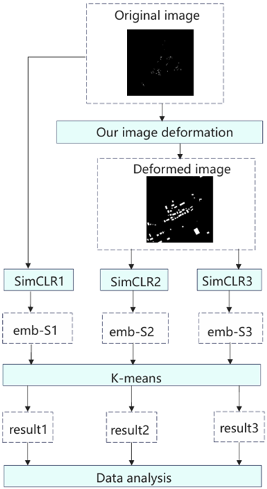
We constructed three SimCLR frameworks: the first using the original SimCLR, the second with our image deformation pipeline, and the third with both our image deformation pipeline and loss function. We refer to them as SimCLR1, SimCLR2, and SimCLR3. Their training processes are shown in
Figure 1. After the training is completed, the operations performed are as shown in
Figure 2. It is worth noting that our image deformation pipeline is applied not only during training but also during testing. The output of each framework was clustered into five clusters. We submitted representative samples of the clustering results to students and faculty at the School of Architecture for scoring, to assess whether the clustering results met our research objectives. We also conducted statistics on specific morphological indicators of the results to illustrate the effectiveness of our loss function.
3.2. Study Area
Urban morphological patterns vary greatly under different cultural and geographical backgrounds. To test the effectiveness and transferability of our method, we selected three vastly different Chinese municipal administrative regions as our research areas.
The reason for choosing Chinese cities is that China and South Korea are the only two major countries that use the concept of a wide-area city. This means that China’s municipal-level administrative regions not only include the central urban areas but also a large number of suburbs and towns surrounding the central areas, covering areas of up to tens of thousands of square kilometers. As mentioned above, if we only focus on the central urban areas filled with buildings, there is no significant difference in the morphological characteristics of building clusters and the overall visual characteristics of the map. Therefore, only when conducting urban morphological discovery in complex and massive datasets do the defects of the original simCLR become fully exposed.
The reason for choosing Shanghai, Beijing, and Chongqing is based on two considerations. Firstly, these three cities are mega-cities with populations exceeding 20 million, providing a sufficiently diverse range of urban morphological types for research. Secondly, these three cities have significant differences in geographical conditions, cultural customs, and urban history. For example, Shanghai is located in the Yangtze River Delta, consisting entirely of plains with an area of 6340 square kilometers. Beijing is situated on the edge of the North China Plain, covering an area of 16,410 square kilometers. The southern half is located in the North China Plain, where the majority of buildings and the population are concentrated, while the northern half is mainly composed of hills with fewer buildings and people. Chongqing is located in the mountainous area of southwestern China, with a vast area of 82,400 square kilometers, but it is mainly composed of hills and mountains, with only a small amount of plain areas distributed in valleys. We believe that the diversity of the research areas will provide stronger support for our research conclusions.
3.2.1. Shanghai, China
Shanghai, as one of China’s most populous and bustling metropolises, has undergone significant urban planning to accommodate its ever-growing population. To make efficient use of its limited space, Shanghai has developed a skyline dominated by towering skyscrapers and high-rise residential buildings, stretching towards the heavens. In an effort to create a more livable urban environment and incorporate natural elements into the concrete jungle, Shanghai’s urban planning emphasizes the integration of green spaces and waterways. There is a stark contrast to the traditional dense, grid-like layouts found in many cities.
Although Shanghai is one of the most bustling cities in the world, the presence of the “cultivated land red line” means that many towns and farmlands still exist in the distant suburbs of Shanghai. These rural areas originate from the agriculture of the Taihu Lake Basin, which has been developed for thousands of years. They are densely populated and often built along water bodies. Due to the division by extensive water networks and scattered farmland, these areas present a highly fragmented landscape.
3.2.2. Beijing, China
Beijing’s urban form is deeply influenced by history. The north–south central axis centered on the Forbidden City runs through the entire city. The blocks in the old city are often regular and symmetrical. This layout reflects the aesthetic of symmetry and the concept of ritual in ancient capital planning. As the city expands, Beijing has formed a road network pattern composed of major ring roads such as the Second Ring Road, Third Ring Road, Fourth Ring Road, and several radial roads. This layout facilitates urban traffic organization and also reflects the characteristics of modern urban planning.
The administrative area of Beijing covers a vast 16,410.54 square kilometers. Like other cities in China, within such a large area, in addition to the central city, there are many suburban areas dominated by towns and rural areas. The architectural style of Beijing’s villages is influenced by traditional Northern Chinese styles, with many adopting the siheyuan (courtyard house) layout. Due to Beijing’s long-standing role as China’s capital and a military stronghold, there are also many functional buildings remaining from ancient times in the suburban areas, such as the Great Wall.
3.2.3. Chongqing, China
Chongqing is a massive city in Southwest China, known as the “Mountain City” due to the fact that 76 percent of its jurisdiction is mountainous terrain. The city’s architecture is predominantly built along the mountains, creating a unique landscape where “mountains are within the city, and the city is on the mountains”. The special natural environment has shaped a unique urban development pattern. Due to the lack of large plains, Chongqing’s urban area has adopted a cluster-type development. Different urban areas are relatively independent and interconnected by transportation networks. The building groups outside the urban area obstructed by mountainous terrain often appear as strip-like or cloud-like distributions, with significantly lower building density compared to the suburban areas of Shanghai and Beijing. Given that Chongqing’s area spans over 80,000 square kilometers, we randomly selected only one-fifth of this area for our experiments.
3.2.4. An Example Showcasing the Impact of Building Density and Scale
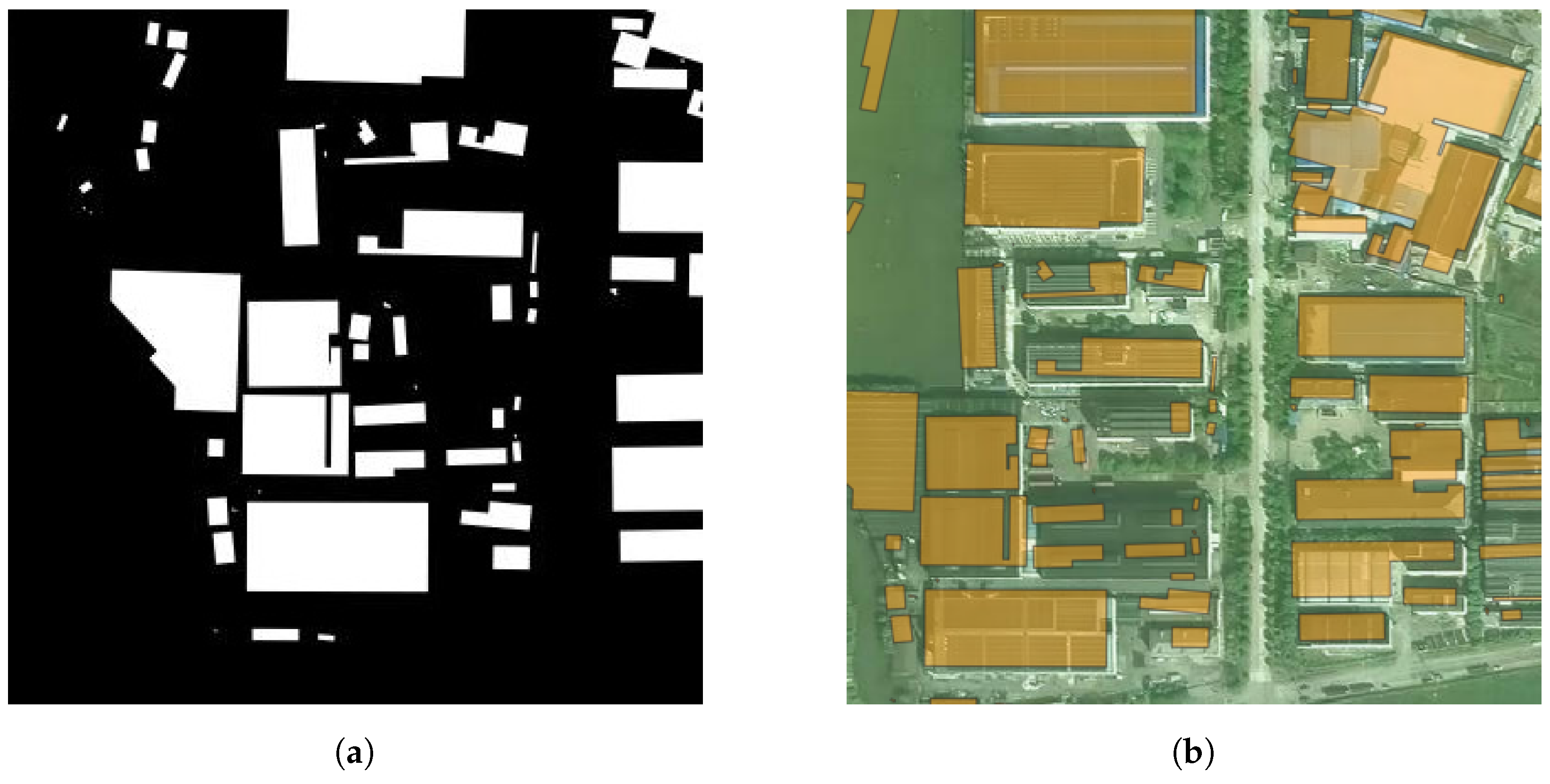
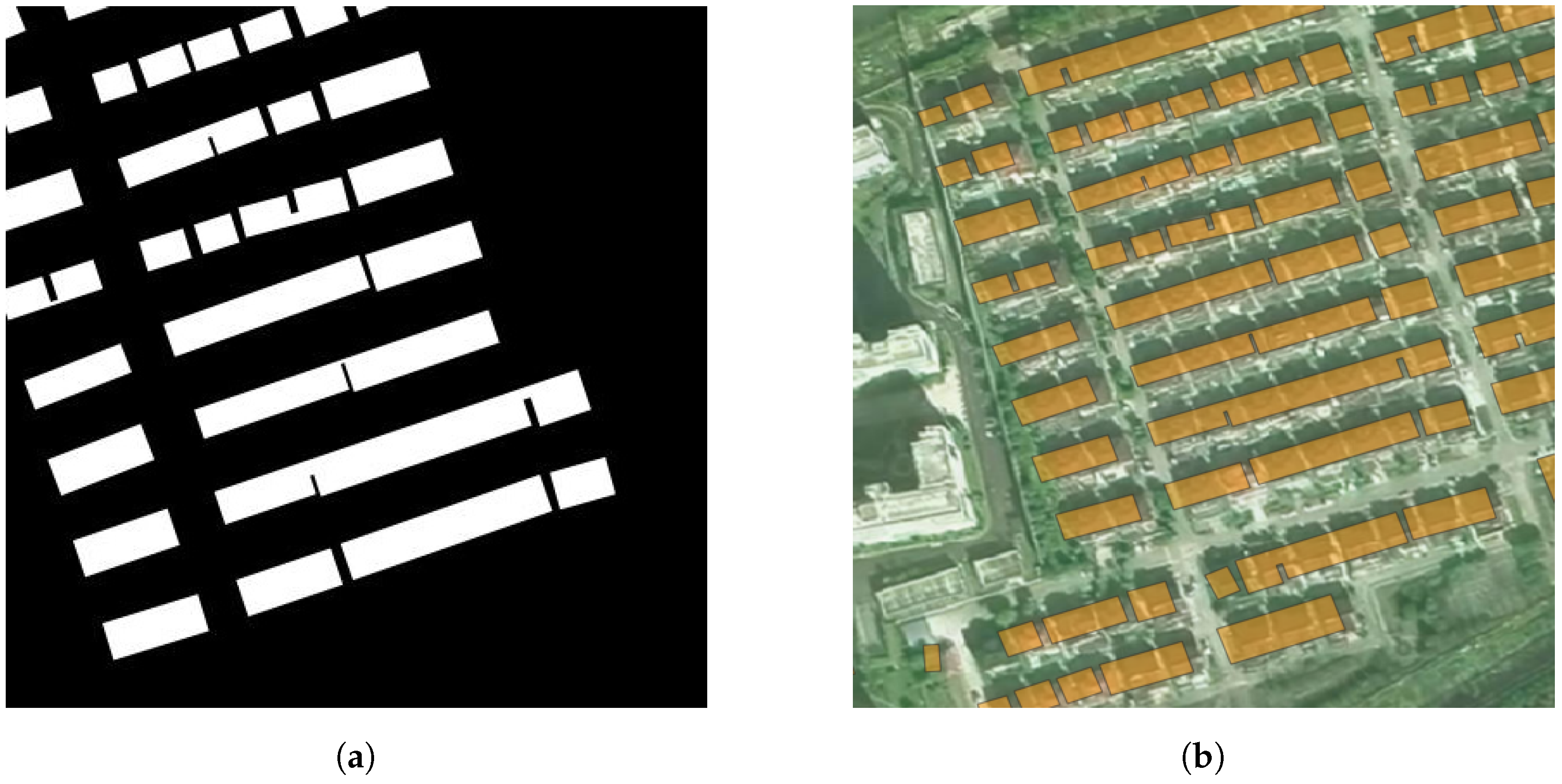
In such complex datasets, the differences between samples are reflected not only in the morphological characteristics of building groups but also in their scale and density. Due to the visual characteristics brought by the distribution and density of building groups being stronger than the morphological characteristics of building groups, many visual neural networks become insensitive to the differences in the characteristics. Shown in
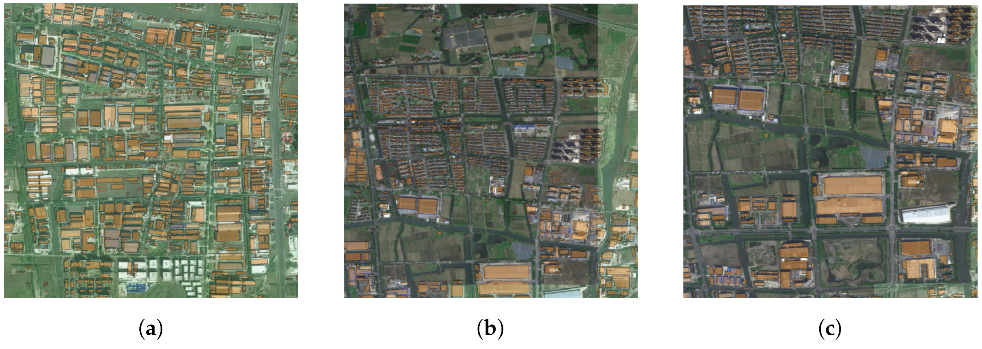
Figure 3a,b are samples from the same city. Sample 1 has more buildings, which are concentrated in the center of the image. In sample 2, there are fewer buildings and they are scattered. These differences result in significant visual distinctions. However, if the building group on the left half of
Figure 3b is enlarged to obtain
Figure 3c, it can be seen that there is a clear similarity in the morphological characteristics of building groups between
Figure 3a,c. It can also be observed from the corresponding satellite maps that both
Figure 4a,c are composed of factories and related supporting buildings. This similarity often contains profound connotations but is often ignored by visual neural networks. As mentioned in the introduction, this is precisely why we need to design a new image deformation pipeline.
Additionally, it can be observed that the upper left corner of
Figure 4b contains a residential area. If raster analysis were used, this residential area would be mixed with the surrounding industrial area in the corresponding Nolli map,
Figure 3b. However, the division method we used, based on administrative boundaries, successfully avoided such mixing.
3.3. Simclr and Our Improvements
3.3.1. The Overview of Contrastive Learning and SimCLR
Contrastive learning is a method focused on extracting meaningful representations through contrasting instance pairs. It leverages the assumption that similar instances should be closer to each other in the learned embedding space, while different instances should be farther apart. By framing learning as a discriminative task, contrastive learning allows models to capture relevant features and similarities in the data.
Self-supervised contrastive learning (SSCL) creates positive and negative pairs (positive pairs are similar samples, negative pairs are dissimilar samples) from unlabeled data without relying on explicit labels. SimCLR is a mainstream SSCL framework that has achieved promising results. The core idea of SimCLR is to maximize the consistency between augmented views of the same instance while minimizing the consistency between views from different instances.
In SimCLR, there are four main processes, which are as follows and are illustrated in
Figure 1 and
Figure 2:
A pipeline of data augmentation operations, denoted as DA. Each original sample s is augmented twice to produce two augmented views and . These augmented views from the same original sample are considered as positive pairs, while those from different original samples are treated as negative pairs.
The next step is to train the encoder network . The encoder network takes the augmented instances as input and maps them to a latent representation space. This means being embedded, .The encoder network is typically a deep neural network architecture, such as a Convolutional Neural Network (CNN) for image data. This network learns to extract and encode high-level representations from the augmented instances, facilitating the distinction between similar and different instances in subsequent steps.
A projection network is used to further refine the learned representations. The projection network takes the output from the encoder network and projects it onto a lower-dimensional space, commonly referred to as the projection or embedding space. This means becoming lower-dimension embedded, .
The contrastive loss function is computed, and gradients are backpropagated to both the encoder network and the projection network. SimCLR employs a specific normalization technique called “normalized temperature-scaled cross-entropy” (NT-Xent) loss. The value of this loss function is positively correlated with the distance between negative pairs and negatively correlated with the distance between positive pairs. The detailed explanation lies in Equation (
3).
3.3.2. Image Deformation Pipeline
Data augmentation typically involves performing random operations on images to create a new image. Common operations include random cropping, color jittering, random flipping, and so on. In the SimCLR, an original sample is augmented twice, resulting in two new samples referred to as the left image and the right image. It is generally assumed that the two new samples created through this operation belong to the same category. These are the so-called positive samples. It is the core assumption of the SimCLR and often holds true in CV research. However, this may not always be the case for our research content because we cannot guarantee that a single plot contains only one type of building group morphology, nor can we ensure that the plot is filled with buildings. The augmented new samples may include multiple types of buildings. They may also not contain any building groups at all. This is precisely the substantial impact of the uneven distribution of building groups mentioned earlier.
To overcome the aforementioned difficulties, we designed an image deformation pipeline. This pipeline replaces the completely random cropping with restricted random cropping. It is necessary to determine the center and width of the cropping step by step (in order to adapt to subsequent operations, the cropped new image is always a square). The specific approach is:
The original image of the building groups is subjected to two dilation and four erosions, resulting in a new image called a mask. This new image roughly matches the distribution of the original building groups but has two characteristics: first, buildings originally located at the edges of the clusters are not covered by the mask, because the number of erosions is greater than the number of dilations; second, small and dense building groups are highlighted compared to larger ones. This is because during dilation, small and dense clusters not only expand into surrounding empty spaces but also fill in their internal gaps.
Points are randomly sampled on the mask as the cropping centers. Since two deformed samples are required, this step involves selecting two cropping centers. We have set a limit of no more than 1024 pixel clusters between the two cropping centers to ensure that the two deformed samples are likely to focus on the same building group with high probability.
Let the median area of the buildings within the plot be denoted as
.
is taken as the minimum value for the cropping width, and
as the maximum value. Their relationship is shown in Equations (
1) and (
2).
We randomly select an integer between and as the cropping width, and the random cropping widths for the two deformations are independent. This approach ensures that the cropped samples always contain an appropriate number of buildings while retaining some randomness to enhance the robustness of the model.
The detailed pseudocode can be found in
Appendix A. Some image materials are shown in
Figure 5. Because we performed color inversion during the image processing, in the following Nolli map, white represents buildings and black represents the background.
After passing through our designed image deformed pipeline, we then randomly flipped and applied random color jitter to the cropped images, and resized them to 224 × 224 pixels, resulting in two usable augmented samples. These two samples always focus on the same building group and are typically filled with enough buildings.
3.3.3. CNN Model
After completing all the image operations, the augmented images need to be input into a CNN model in batches. The CNN model will convert the images into feature vectors and will be continuously optimized during the training process. The CNN model we chose is an improved res50 model, with specific modifications including:
We adjusted the model’s input to single channel because our input samples are all grayscale images.
We adjusted the model’s output to a feature vector of length 128, which serves as the image’s feature representation.
Our batch contains 4 original samples, which means 8 augmented samples after augmentation. After passing through the model, we obtain 8 feature vectors of length 128. These 8 feature vectors are paired according to the original samples. Pairs of samples from the same original sample are considered the same class (positive samples pairs), while any two feature vectors from different original samples are considered different classes (negative samples pairs).
3.3.4. Loss Function
During the training process, an appropriate loss function is needed to optimize the model parameters. The loss function used in SIM is called NT-Xent loss. The specific definition is as follows:
where:
are the feature representations of two augmented views of the same data point;
is the similarity measure between feature vectors a and b;
is the temperature parameter, which adjusts the sensitivity of the loss function;
N is half of the batch size, since each data point has two views;
is the indicator function, which is 1 if and 0 otherwise.
The basic principle of this loss function is to minimize the distance between samples of the same class and maximize the distance between samples of different classes. However, this principle may not always be reasonable, as even two augmented samples from different original samples could potentially belong to the same class. In computer vision (CV), this deficiency is difficult to overcome because no additional information about the images is available. However, in morphology, it is possible to roughly estimate the similarity of the original samples through morphometric analysis. Taking this into account, we calculated the proportion of building area for each original sample based on the building vector data of the original samples, denoted as
p. Then, we made a simple optimization to the loss function. The specific definition is as follows:
where:
P is the indicator function that considers p. If , P is 0; if 0 < , P is 0.1; if , P is 0.5; otherwise, P is 1.
Clearly, this is a simple calculation method that can only roughly distinguish between urban centers, suburbs, and rural areas. Even so, our experiments have proven the effectiveness of this strategy. It successfully uses morphological strategies to guide the optimization of the visual neural network.
4. Experiment and Results
4.1. Experimental Parameters and Expected Results
To demonstrate the effectiveness of our method, we simultaneously constructed three pipelines: the first using the original SimCLR, the second with our image deformation pipeline, and the third with both our image deformation pipeline and loss function. We refer to them as SimCLR1, SimCLR2, and SimCLR3. They all have the same parameters with a weight decay of
, a minibatch size
N of 4, a learning rate of
, and a temperature parameter
of
. The optimizer used was Adam, which is a widely used optimization algorithm in deep learning [
34]. It combines the ideas of momentum methods (Momentum) and RMSProp, aiming to adjust the learning rate for each parameter by computing the first-order and second-order moment estimates of the gradients, thereby achieving more efficient network training. The training process spans 30 epochs. Expected results include:
In SimCLR1, due to the lack of a deformation pipeline to enhance the morphological characteristics of building clusters, the final classification results tend to group samples with similar overall visual effects together. In terms of data, samples with similar proportions of built-up area are grouped together. This is because the building area ratio p is one of the key indicators that most affects the overall visual effect.
In SimCLR2, the deformation pipeline enhances the morphological characteristics of building clusters. The augmented samples always focus on a certain cluster of buildings, and the overall visual effect of the original samples is no longer emphasized. Therefore, the final clustering results will group those similar clusters of buildings together, while the p within each cluster will become discrete.
In SimCLR3, due to the presence of the deformation pipeline, building clusters with similar morphologies are still grouped together. However, because we have added some terms related to p in the loss function, the values of p within each cluster will be more concentrated, even though the CNN at this point cannot perceive the overall visual effect of the original samples.
4.2. Clustering Results and Their Evaluation
We divided the city according to the administrative village boundaries, with each village’s Nolli map serving as a single sample. The number of samples for each experiment ranged between 1000 and 2000. The dataset was used for training as shown in
Figure 1, and for testing as shown in
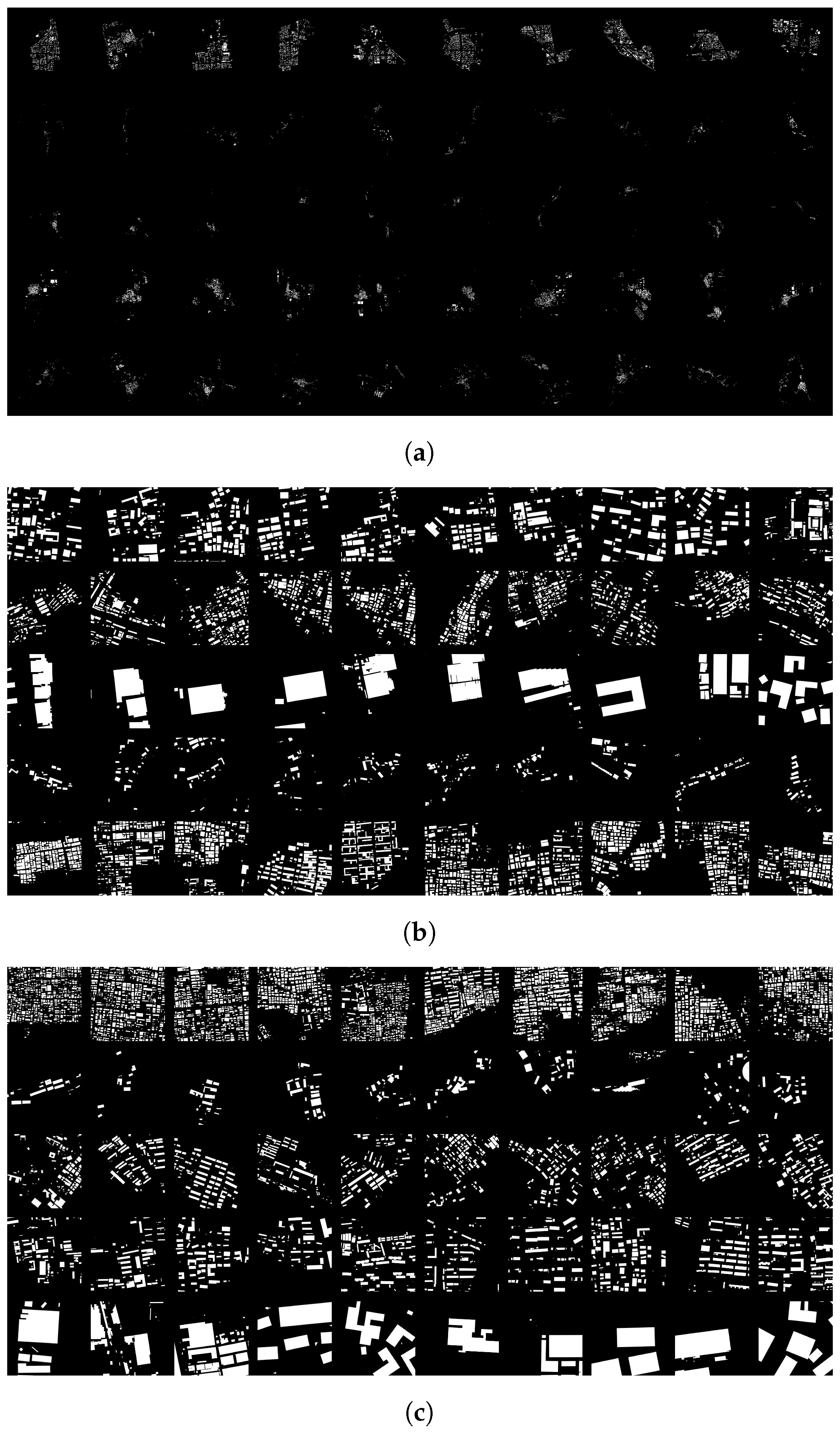
Figure 2. For the embeddings output by the CNN, we used the K-means clustering technique with five clusters. Subsequently, we selected the 10 samples closest to the cluster center for each category as representatives of that category. The clustering results for Shanghai are shown in
Figure 6. Each row in every subplot represents a clustering cluster. It can be observed that SimCLR1 tends to cluster according to the distribution and density of building groups but ignores the morphological characteristics. However, SimCLR2 and SimCLR3 well satisfy our research purposes. The results for Beijing and Chongqing are included in
Appendix A. They also have the same characteristics.
We submitted the clustering results to some students and an urban planner from the School of Architecture, asking them to evaluate whether these clustering results met our research objectives: to achieve a classification of urban forms primarily based on the morphological characteristics of building groups. Six people participated in the scoring. Each person gave a score between 0 and 10 for each clustering result. The final scoring table is shown in
Table 1:
It can be observed that SimCLR2 and SimCLR3 are generally considered to have better results than SimCLR1. This advantage is obvious in Beijing and Chongqing but less so in Shanghai. This is because Shanghai has a high proportion of built-up areas, which does not perfectly align with our assumptions about the dataset. In contrast, Beijing and Chongqing have a lower proportion of built-up areas, which can be seen in
Figure 7.
4.3. Analysis of Clustering Results
To further demonstrate the effectiveness of our loss function, we calculated the dispersion degree of the building area ratio of the clustering results. The specific process is as follows:
Using random initial cluster centers for k-means with clusters of five. Extracting the 10 samples closest to the cluster centers for each cluster.
Calculating the variance of the building area ratio for these 10 samples as the dispersion degree for a cluster.
Adding the variances of the five clusters belonging to the same clustering result. The sums from SimCLR1, SimCLR2, and SimCLR3 are called D1, D2, and D3.
We repeated the above experimental process ten times, The statistic is shown in
Table 2. It can be seen that D3 is almost always less than D2. This fully demonstrates that our loss function successfully guided the optimization of the model, making it more inclined to cluster samples with a similar building area ratio. Moreover, this guidance is established on the premise of not affecting the performance of basic tasks.
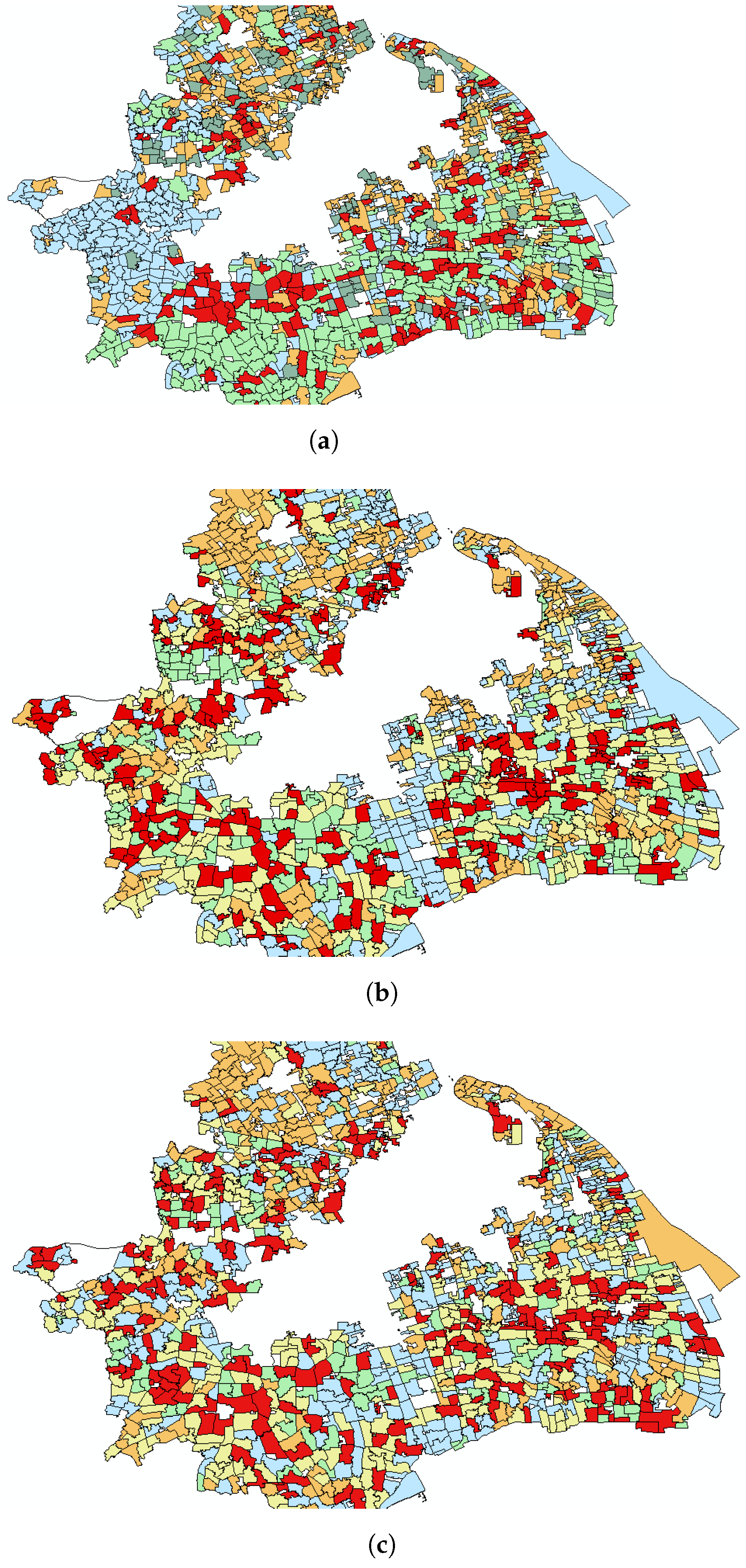
Figure 8 displays the geographic distribution of the clustering in Shanghai (due to dataset defects, there are some blank spaces in the center of the graph). In each image, plots of the same color belong to the same clustering. It can be observed that
Figure 8b,c are quite similar. However,
Figure 8a is distinctly different from the other two. In
Figure 8a, plots that are geographically close to each other are more likely to be grouped into the same clustering. This proves that SimCLR1 has a strong focus on the distribution of building groups, because there is a high correlation between geographic location and the distribution of building groups: urban plots are always filled with dense building groups, while suburban plots tend to have only sparse and separated building groups.
Table 2 also confirms our viewpoint. D1 is much smaller than that of the other two, which fully indicates that SimCLR1 has a strong tendency to cluster samples with a similar building density. This necessarily leads to the neglect of the morphological characteristics of the building groups.
4.4. Specific Analysis of the Discovered Urban Forms
We believe that both SimCLR2 and SimCLR3 have successfully completed the discovery of urban forms based on the morphological characteristics of building groups, and the urban forms they have identified are similar. The following is a specific analysis of these urban forms, using the clustering results of SimCLR3 for Shanghai as an example.
The first type of form, as shown in
Figure 9, corresponds to the first row in
Figure 6c. This form consists of sparse buildings with small floor areas, typically found in rural areas. Sometimes it exhibits a linear distribution pattern, which is because rural buildings are often arranged along the road network.
The second type of form, as shown in
Figure 10, corresponds to the second row in
Figure 6c. This form reveals the presence of mega-structures, which are distributed both in suburban and urban areas. Mega-structures often serve specific functions, for example, as museums, factories, and others.
The third type of form, as shown in
Figure 11, corresponds to the third row in
Figure 6c. This form has a certain degree of planning, but the building floor areas are uneven. It typically represents a multi-functional urban block that encompasses various types of buildings, including production facilities, commercial spaces, and residential areas. Such a form is more prevalent in the suburbs and often serves as a hub for small and micro enterprises.
The fourth type of form, as shown in
Figure 12, corresponds to the fourth row in
Figure 6c. This form is composed of neatly arranged elongated buildings, representing well-organized residential communities. These residential areas were often constructed in the last few decades, in line with China’s rapid urbanization. They are typically located in suburban regions.
The fifth type of form, as shown in
Figure 13, corresponds to the fifth row in
Figure 6c. This form tends to be chaotic, appearing both in the peripheral areas and the central areas of the city. Although it lacks formal planning, it may have a long history and carry unique cultural connotations.
4.5. Summary of the Result
Overall, in this study, three different SimCLR frameworks were applied to urban morphological discovery on the same dataset. The experiment demonstrated that SimCLR1 can only process the global visual features of each original sample, tending to cluster samples with similar geographical locations and proportions of built-up area p, and it fails to effectively accomplish the task of urban morphological discovery. Both SimCLR2 and SimCLR3 performed better in urban morphological discovery. SimCLR2, not focusing on the global visual features of the original samples, did not cluster samples with similar p. Although SimCLR3 also did not focus on the global visual features of the original samples, it successfully clustered samples with similar p due to the addition of a coefficient related to p in the loss function.
The experimental results proved that the image deformation pipeline designed in this study successfully guided the model to focus on extracting the morphological characteristics of building clusters, and the loss function integrated with morphometric indicators successfully achieved specific guidance for the model.
5. Discussion
In this section, we will discuss several key technical points of the method we propose. First is our image deformation pipeline. The purpose of data augmentation is to maintain the image category while changing the image content. The CV discipline hopes that its algorithms can be applied to all types of images, so the data augmentation methods they use are relatively conservative and universal, such as random cropping, random flipping, random adjusting of color tones, etc. However, in morphological research, we do not need the model to have strong universality, but only need the model to focus on the visual features we are concerned with. Based on this concept, we designed an image deformation pipeline specifically suitable for our research content. This improvement is very effective, allowing the model to ignore the visual features we are not concerned with (the distribution of building groups) and focus on identifying the characteristics we are interested in. In fact, this recognition pattern is also closer to human cognition: when we are asked to pay attention to details, we often focus our attention on small areas. We believe that this design concept should also be widely applicable to other morphological studies.
Secondly, our improved loss function. The purpose of doing this is to integrate morphological prior knowledge into the model. We are not the only ones trying to achieve this goal. For example, Ref. [
14] uses morphological indicators to fill in maps for the same purpose. Compared to their approach, our method is clearly more interpretable. By changing the loss function, we make the model “recognize” that samples with large differences in morphological indicators need to be further apart from each other, thus making the model’s optimization more efficient.
The image deformation pipeline designed in this study allowed the model to focus on extracting the morphological characteristics of building clusters. Moreover, during clustering, the model clustered the augmented views rather than the original samples, which did not interfere with the research objective of urban form discovery. However, if researchers aim to study the similarity between original samples, this model has a limitation: it cannot perceive the global visual features of the original samples. In subsequent research, we addressed this issue through multiple sampling methods. We performed 20 random augmentations for each original sample and then clustered these numerous augmented views. Finally, we statistically analyzed the clustering results of the augmented views for each original sample to determine the similarity between the original samples. While this approach achieved global perception of the original samples, it introduced a significant computational load, which may not be the most efficient method.
6. Conclusions
In this study, we conducted urban form discovery on a vast and complex dataset based on administrative village units, and introduced some technological innovations for this purpose. We designed an image deformation pipeline which ensures that the augmented images focus on a building group and contain an appropriate number of buildings. We also designed a loss function that incorporates morphological indicators, which allows the model to “recognize” the similarity between samples for more controllable optimization.
These technological innovations were integrated into the SimCLR framework. Subsequently, the improved SimCLR and the original SimCLR were applied to three distinctly different Chinese cities with varying styles. Some representative urban types were identified. Experimental results and data analysis demonstrated the effectiveness of our method.
Our method demonstrates better visual feature extraction capabilities compared to traditional morphometrics. It also offers improved results and controllability compared to the original SimCLR. In particular, our optimization of the loss function has introduced a new concept that integrates morphometrics with computer vision. This approach can guide visual neural networks to learn specific morphometric knowledge. We believe it has a wide range of potential applications.
Although the study has achieved good results, there are still some aspects that could be refined. Firstly, we only used a simple building density to improve the loss function. The potential of this optimization concept may be much greater than the effect it demonstrates in this study. This is because we can use more morphological indicators to analyze the similarity between samples, thus better guiding the CNN model to optimize. Theoretically, it can also be applied to many other directions of morphological research, such as road network classification, landscape classification, etc. Secondly, improvements to the original images could also yield positive feedback. In this study, only Nolli maps were used as single-channel images, which actually simplifies the complex attributes of buildings. Therefore, it is necessary to expand the channels of the images to provide richer information, such as adding building height maps and population density maps to form three-channel images. Thirdly, more comparative experiments and richer evaluation indicators will help to comprehensively validate the effectiveness of this study, and provide a more thorough assessment of the potential impact of our image deformation pipeline and refined loss function on the contrastive learning framework.
Author Contributions
Conceptualization, Chunliang Hua and Mengyuan Niu; methodology, Qiao Wang; software, Chunliang Hua; validation, Chunliang Hua; investigation, Daijun Chen; resources, Daijun Chen; writing—original draft preparation, Chunliang Hua; writing—review and editing, Qiao Wang; visualization, Chunliang Hua; supervision, Lizhong Gao and Junyan Yang. All authors have read and agreed to the published version of the manuscript.
Funding
This research is supported by the National Key R&D Program of China (2024YFC3807900), and partially supported by Project Four of the National Natural Science Foundation of China (NSFC) Major Program, Prototype Construction of Carbon Neutrality Building Technology for High Density Urban Environment, Project Number: 52394224.
Data Availability Statement
The original contributions presented in this study are included in the article. Further inquiries can be directed to the corresponding author(s).
Acknowledgments
Thank you to the six raters who scored our experimental results. As professionals, their scores provided strong support for the conclusions of the paper. Some detailed information about them can be found in
Appendix A.
Conflicts of Interest
The authors declare no conflicts of interest.
Abbreviations
The following abbreviations are used in this manuscript:
| CNN | Convolutional Neural Network |
| NT-Xent Loss | Normalized Temperature-Scaled Cross-Entropy Loss |
| SimCLR | Three Simple Framework for Contrastive Learning of Representations |
Appendix A. Experimental Data and Pseudo-Code
Table A1.
The scores for clustering results.
Table A1.
The scores for clustering results.
| | | Scores Between 0 and 10 |
|---|
| | | rater1 | rater2 | rater3 | rater4 | rater5 | rater6 |
|---|
| Beijing | SimCLR1 | 2 | 6 | 6 | 6 | 6 | 6 |
| SimCLR2 | 7.5 | 8 | 9 | 7 | 7 | 10 |
| SimCLR3 | 7.5 | 9 | 6 | 8 | 8 | 8 |
| Shanghai | SimCLR1 | 2 | 8 | 7 | 8 | 7 | 5 |
| SimCLR2 | 8 | 7 | 8 | 7 | 8 | 8 |
| SimCLR3 | 7 | 7 | 7 | 7 | 7 | 9 |
| Chongqing | SimCLR1 | 1 | 6 | 4 | 7 | 6 | 6 |
| SimCLR2 | 3 | 7 | 6 | 7 | 8 | 8 |
| SimCLR3 | 6 | 8 | 9 | 8 | 8 | 9 |
Personal information of raters:
Rater1: Second-year Ph.D. student in Urban and Rural Planning.
Rater2: Fourth-year Ph.D. student in Urban and Rural Planning.
Rater3: Fourth-year Ph.D. student in Landscape Architecture.
Rater4: Third-year Ph.D. student in Urban and Rural Planning.
Rater5: Intermediate urban planner.
Rater6: Fifth-year Ph.D. student in Urban and Rural Planning.
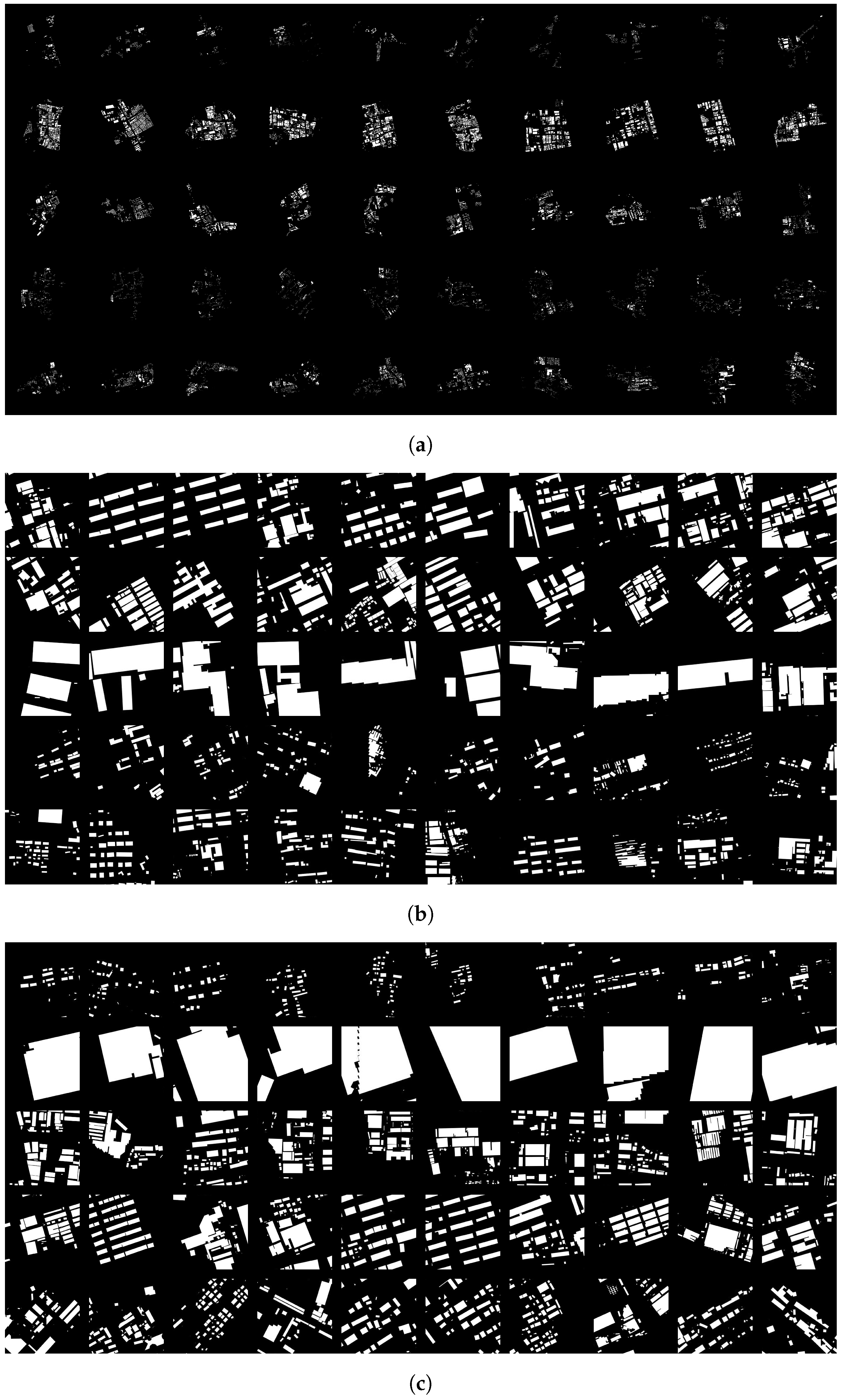
Figure A1.
Clustering results for Beijing. (a) Results of SimCLR1; (b) Results of SimCLR2; (c) Results of SimCLR3.
Figure A1.
Clustering results for Beijing. (a) Results of SimCLR1; (b) Results of SimCLR2; (c) Results of SimCLR3.
Figure A2.
Clustering results for Chongqing. (a) Results of SimCLR1; (b) Results of SimCLR2; (c) Results of SimCLR3.
Figure A2.
Clustering results for Chongqing. (a) Results of SimCLR1; (b) Results of SimCLR2; (c) Results of SimCLR3.
| Algorithm A1 Image deformation pipeline |
Input: original image, the median area of the buildings denoted as area_med Output: L_cropped_image and R_cropped_image
- 1:
Define the kernel for morphological operations - 2:
kernel_size ← 15 - 3:
kernel ← np.ones((kernel_size, kernel_size), np.uint8) - 4:
Obtain the mask from the original image - 5:
dilated_image ← cv2.dilate(original_image, kernel, iterations=2) - 6:
eroded_image ← cv2.erode(dilated_image, kernel, iterations=4) - 7:
mask ← eroded_image - 8:
mask[mask > 0] ← 255 - 9:
functionfind_random_pixel_with_value_255() - 10:
while True do - 11:
y ← random.randint(0, mask.shape[0] − 1) - 12:
x ← random.randint(0, mask.shape[1] − 1) - 13:
if mask[y, x] == 255 then - 14:
return (x, y) - 15:
end if - 16:
end while - 17:
end function - 18:
functioncalculate_crop_bounds() - 19:
top ← max(center[1] − side_length // 2, 0) - 20:
bottom ← min(center[1] + side_length // 2, mask.shape[0]) - 21:
left ← max(center[0] − side_length // 2, 0) - 22:
right ← min(center[0] + side_length // 2, mask.shape[1]) - 23:
return (top, bottom, left, right) - 24:
end function - 25:
Select the first center point, then select the second center point with distance constraint - 26:
L_center ← find_random_pixel_with_value_255(mask) - 27:
while True do - 28:
R_center ← find_random_pixel_with_value_255(mask) - 29:
distance ← sqrt((R_center[0] − L_center[0] + (R_center[1] − L_center[1]) - 30:
if distance < 1024 then - 31:
break - 32:
end if - 33:
end while - 34:
Generate random side lengths within the specified boundaries - 35:
min_side_length ← 10 * sqrt(area_med) - 36:
max_side_length ← 2 * min_side_length - 37:
L_side_length ← random.randint(min_side_length, max_side_length) - 38:
R_side_length ← random.randint(min_side_length, max_side_length) - 39:
Crop the original image based on the calculated bounds - 40:
L_bounds ← calculate_crop_bounds(L_center, L_side_length) - 41:
R_bounds ← calculate_crop_bounds(R_center, R_side_length) - 42:
L_cropped_image ← original_image[L_bounds[0]:L_bounds[1], L_bounds[2]:L_bounds[3]] - 43:
R_cropped_image ← original_image[R_bounds[0]:R_bounds[1], R_bounds[2]:R_bounds[3]]
|
References
- Hillier, B.; Hanson, J. The Social Logic of Space; Cambridge University Press: Cambridge, UK, 1984. [Google Scholar] [CrossRef]
- Trancik, R. Finding Lost Space: Theories of Urban Design; Van Nostrand Reinhold: New York, NY, USA, 1986. [Google Scholar]
- Scheck, E.; Binn, A.; Dörk, M.; Ledermann, F. A Contemporary Nolli Map: Using OpenStreetMap Data to Represent Urban Public Spaces. Abstr. ICA 2023, 6, 223. [Google Scholar] [CrossRef]
- Ji, H.; Ding, W. Mapping urban public spaces based on the Nolli map method. Front. Archit. Res. 2021, 10, 540–554. [Google Scholar] [CrossRef]
- Taubenböck, H.; Debray, H.; Qiu, C.; Schmitt, M.; Wang, Y.; Zhu, X. Seven city types representing morphologic configurations of cities across the globe. Cities 2020, 105, 102814. [Google Scholar] [CrossRef]
- Dimitrovski, I.; Kitanovski, I.; Kocev, D.; Simidjievski, N. Current trends in deep learning for Earth Observation: An open-source benchmark arena for image classification. ISPRS J. Photogramm. Remote Sens. 2023, 197, 18–35. [Google Scholar] [CrossRef]
- Zhang, P.; Ke, Y.; Zhang, Z.; Wang, M.; Li, P.; Zhang, S. Urban Land Use and Land Cover Classification Using Novel Deep Learning Models Based on High Spatial Resolution Satellite Imagery. Sensors 2018, 18, 3717. [Google Scholar] [CrossRef]
- Zhang, R.; Wang, F.; Li, W. Deep Learning for Remote Sensing Data: A Technical Review on the State of the Art. ISPRS J. Photogramm. Remote Sens. 2016, 115, 119–139. [Google Scholar] [CrossRef]
- Ratti, C.; Richens, P. Raster Analysis of Urban Form. Environ. Plan. B Plan. Des. 2004, 31, 297–309. [Google Scholar] [CrossRef]
- Chen, T.; Kornblith, S.; Norouzi, M.; Hinton, G. A simple framework for contrastive learning of visual representations. arXiv 2020, arXiv:2002.05709. [Google Scholar]
- Yin, J.; Dong, J.; Hamm, N.A.; Li, Z.; Wang, J.; Xing, H.; Fu, P. Integrating remote sensing and geospatial big data for urban land use mapping: A review. Int. J. Appl. Earth Obs. Geoinf. 2021, 103, 102514. [Google Scholar] [CrossRef]
- Ghamisi, P.; Rasti, B.; Yokoya, N.; Wang, Q.; Hofle, B.; Bruzzone, L.; Bovolo, F.; Chi, M.; Anders, K.; Gloaguen, R.; et al. Multisource and Multitemporal Data Fusion in Remote Sensing: A Comprehensive Review of the State of the Art. IEEE Geosci. Remote Sens. Mag. 2019, 7, 6–39. [Google Scholar] [CrossRef]
- Chen, Y.; He, C.; Guo, W.; Zheng, S.; Wu, B. Mapping Urban Functional Areas Using Multisource Remote Sensing Images and Open Big Data. IEEE J. Sel. Top. Appl. Earth Obs. Remote Sens. 2023, 16, 7919–7931. [Google Scholar] [CrossRef]
- Wang, J.; Huang, W.; Biljecki, F. Learning visual features from figure-ground maps for urban morphology discovery. Comput. Environ. Urban Syst. 2024, 109, 102076. [Google Scholar] [CrossRef]
- Bobkova, E.; Berghauser Pont, M.; Marcus, L. Towards analytical typologies of plot systems: Quantitative profile of five European cities. Environ. Plan. B Urban Anal. City Sci. 2021, 48, 604–620. [Google Scholar] [CrossRef]
- Joshi, M.Y.; Rodler, A.; Musy, M.; Guernouti, S.; Cools, M.; Teller, J. Identifying Urban Morphological Archetypes for Microclimate Studies Using a Clustering Approach. Build. Environ. 2019, 158, 106–118. [Google Scholar] [CrossRef]
- Li, N.; Quan, S.J. Identifying urban form typologies in Seoul using a new Gaussian mixture model-based clustering framework. Environ. Plan. B Urban Anal. City Sci. 2023, 50, 2342–2358. [Google Scholar] [CrossRef]
- Chen, T.H.K.; Qiu, C.; Schmitt, M.; Zhu, X.X.; Sabel, C.E.; Prishchepov, A.V. Mapping horizontal and vertical urban densification in Denmark with Landsat time-series from 1985 to 2018: A semantic segmentation solution. Remote Sens. Environ. 2020, 251, 112096. [Google Scholar] [CrossRef]
- Vanderhaegen, S.; Canters, F. Mapping urban form and function at city block level using spatial metrics. Landsc. Urban Plan. 2017, 167, 399–409. [Google Scholar] [CrossRef]
- Lemoine-Rodrguez, R.; Inostroza, L.; Zepp, H. The global homogenization of urban form. An assessment of 194 cities across time. Landsc. Urban Plan. 2020, 204, 103949. [Google Scholar] [CrossRef]
- Fleischmann, M.; Feliciotti, A.; Romice, O.; Porta, S. Methodological foundation of a numerical taxonomy of urban form. Environ. Plan. B Urban Anal. City Sci. 2022, 49, 1283–1299. [Google Scholar] [CrossRef]
- Fleischmann, M.; Arribas-Bel, D. Geographical characterisation of British urban form and function using the spatial signatures framework. Sci. Data 2022, 9, 546. [Google Scholar] [CrossRef]
- Fang, Z.; Jin, Y.; Zheng, S.; Zhao, L.; Yang, T. UrbanClassifier: A deep learning-based model for automated typology and temporal analysis of urban fabric across multiple spatial scales and viewpoints. Comput. Environ. Urban Syst. 2024, 111, 102132. [Google Scholar] [CrossRef]
- Chen, W.; Huang, H.; Liao, S.; Gao, F.; Biljecki, F. Global urban road network patterns: Unveiling multiscale planning paradigms of 144 cities with a novel deep learning approach. Landsc. Urban Plan. 2024, 241, 104901. [Google Scholar] [CrossRef]
- Krizhevsky, A.; Sutskever, I.; Hinton, G.E. ImageNet classification with deep convolutional neural networks. In Advances in Neural Information Processing Systems; Association for Computing Machinery: New York, NY, USA, 2012; pp. 1097–1105. [Google Scholar] [CrossRef]
- Wang, Z.; Yu, Y.; Li, D.; Wan, Y.; Li, M. Colorful Image Colorization with Classification and Asymmetric Feature Fusion. Sensors 2022, 22, 8010. [Google Scholar] [CrossRef] [PubMed]
- LeCun, Y.; Bottou, L.; Bengio, Y.; Haffner, P. Gradient-based learning applied to document recognition. Proc. IEEE 1998, 86, 2278–2324. [Google Scholar] [CrossRef]
- Bengio, Y.; Courville, A.; Vincent, P. Representation Learning: A Review and New Perspectives. IEEE Trans. Pattern Anal. Mach. Intell. 2013, 35, 1798–1828. [Google Scholar] [CrossRef]
- Goodfellow, I.; Bengio, Y.; Courville, A. Deep Learning; Autoencoders; MIT Press: Cambridge, MA, USA, 2016; Chapter 14. [Google Scholar]
- Moosavi, V. Urban morphology meets deep learning: Exploring urban forms in one million cities, town and villages across the planet. arXiv 2017, arXiv:1709.02939. [Google Scholar]
- Cai, J.; Chen, Y. A novel unsupervised deep learning method for the generalization of urban form. Geo-Spat. Inf. Sci. 2022, 25, 568–587. [Google Scholar] [CrossRef]
- Khosla, P.; Teterwak, P.; Wang, C.; Jaiswal, A.; Fei-Fei, L. Supervised Contrastive Learning. arXiv 2020, arXiv:2004.11362. [Google Scholar]
- Stojnic, V.; Risojevic, V. Self-Supervised Learning of Remote Sensing Scene Representations Using Contrastive Multiview Coding. In Proceedings of the 2021 IEEE/CVF Conference on Computer Vision and Pattern Recognition Workshops (CVPRW), Nashville, TN, USA, 19–25 June 2021; pp. 1182–1191. [Google Scholar] [CrossRef]
- Kingma, D.; Ba, J. Adam: A Method for Stochastic Optimization. Comput. Sci. arXiv 2014, arXiv:1412.6980. [Google Scholar]
| Disclaimer/Publisher’s Note: The statements, opinions and data contained in all publications are solely those of the individual author(s) and contributor(s) and not of MDPI and/or the editor(s). MDPI and/or the editor(s) disclaim responsibility for any injury to people or property resulting from any ideas, methods, instructions or products referred to in the content. |
© 2025 by the authors. Published by MDPI on behalf of the International Society for Photogrammetry and Remote Sensing. Licensee MDPI, Basel, Switzerland. This article is an open access article distributed under the terms and conditions of the Creative Commons Attribution (CC BY) license (https://creativecommons.org/licenses/by/4.0/).


