Explainable Spatio-Temporal Inference Network for Car-Sharing Demand Prediction

Abstract

Efficient resource allocation in car-sharing systems relies on precise predictions of demand. Predicting vehicle demand is challenging due to the interconnections of temporal, spatial, and spatio-temporal features. This paper presents the Explainable Spatio-Temporal Inference Network (eX-STIN), a new approach that improves upon our prior Unified Spatio-Temporal Inference Prediction Network (USTIN) model. It offers a comprehensive framework for the integration of various data. The eX-STIN model enhances the previous one by utilizing Ensemble Empirical Mode Decomposition (EEMD), which results in refined feature extraction. It uses Minimum Redundancy Maximum Relevance (mRMR) to find features that are relevant and not redundant, and Shapley Additive Explanations (SHAP) to show how each feature affects the model’s predictions. We conducted extensive experiments that use real car-sharing data to thoroughly evaluate the efficacy of the eX-STIN model. The studies revealed the model’s ability to accurately represent the relationships among temporal, spatial, and spatio-temporal features, outperforming the state-of-the-art models. Moreover, the experiments revealed that eX-STIN exhibits enhanced predictive accuracy compared to the USTIN model. This proposed approach enhances both the accuracy of demand prediction and the transparency of resource allocation decisions in car-sharing services.

1. Introduction

Urban mobility has undergone substantial changes due to the emergence of shared transportation services, notably ride-sharing platforms like Didi, Lyft, InDrive, and Uber. In 2020, Uber recorded over 5 billion orders (Investor 2021), while Didi facilitated an average of 50 million trips every day (Xu Wei 2020) [1]. Alongside the growth of ride hailing, car-sharing services such as Zipcar and Turo have emerged as viable substitutes for private vehicle ownership. These services offer flexible, on-demand access to a shared fleet, encouraging economical and ecologically friendly transportation alternatives [2]. Car-sharing systems enhance urban sustainability and are pivotal in addressing climate change by reducing CO₂ emissions, decreasing urban congestion, and reducing dependence on private vehicles.

Optimizing car-sharing operations requires accurate demand prediction that accounts for temporal, spatial, and spatio-temporal variations influencing vehicle usage patterns [3]. Unlike private vehicle demand, which is primarily driven by individual commuting behaviors, or ride-hailing services, which respond dynamically to real-time service requests, car-sharing demand is shaped by long-term mobility trends, vehicle accessibility, and external factors. Temporal features, including daily commuting patterns, peak-hour fluctuations, weekends, and seasonal variations, play a crucial role in determining demand. Spatial factors, such as the proximity of car-sharing stations to public transit hubs, business districts, and residential areas, further influence vehicle utilization. Spatio-temporal dependencies, such as the impact of weather conditions, introduce additional complexity, necessitating advanced predictive modeling. Without precise demand prediction that integrates these multidimensional influences, car-sharing operators face challenges in fleet allocation, service reliability, and user satisfaction. Incorporating predictive models that effectively capture temporal, spatial, and spatio-temporal relationships can improve vehicle availability, operational efficiency, and service performance, fostering a more adaptive and sustainable urban mobility ecosystem [4].

Although extensive research has been conducted on mobility demand prediction, car-sharing demand prediction remains complex due to its reliance on multiple interacting factors. Traditional statistical models, such as autoregressive integrated moving average (ARIMA) and support vector regression (SVR), have been widely applied for short-term demand prediction but often struggle to capture nonlinear and spatio-temporal dependencies in mobility data [3,5]. Machine learning techniques, including random forests and gradient boosting methods, have demonstrated improved predictive accuracy but lack generalizability across different urban environments [6]. Deep learning models, such as convolutional neural networks (CNNs) and recurrent neural networks (RNNs), have proven effective in capturing complex spatial and temporal dependencies in shared mobility data [7]. However, their lack of interpretability limits their practical applicability, making it difficult for urban planners and fleet operators to derive meaningful insights [8]. Existing studies have predominantly analyzed either spatial or temporal relationships in isolation, overlooking the critical role of spatio-temporal interactions in modeling car-sharing demand variations [3]. The lack of integration of these dependencies results in suboptimal fleet management, increased operational costs, and reduced service efficiency. Given these challenges, a more advanced and interpretable demand prediction framework is necessary, one that comprehensively captures temporal, spatial, and spatio-temporal dynamics to optimize shared mobility services [2,9].

This study introduces the Explainable Spatio-Temporal Inference Network (eX-STIN), a deep learning framework developed to enhance both the accuracy and interpretability of car-sharing demand prediction. Building upon the Unified Spatio-Temporal Inference Prediction Network (USTIN), the model retains core architectural components comprising temporal, spatial, and spatio-temporal units to effectively model complex demand dynamics [3]. To further improve performance, eX-STIN integrates Ensemble Empirical Mode Decomposition (EEMD) for feature extraction and Minimum Redundancy Maximum Relevance (mRMR) for selecting the most informative features. Additionally, Shapley Additive Explanations (SHAP) is employed to quantify feature contributions, providing transparent insights into the model’s predictions and supporting informed decision-making. eX-STIN is specifically designed to overcome key limitations observed in existing predictive models. Many deep learning approaches are limited by their black-box nature, which limits trust and usability in operational contexts [10]. Moreover, the absence of embedded feature selection mechanisms often leads to overfitting and reduced generalizability [11]. Conventional models also struggle to fully capture the intricate dependencies that characterize car-sharing systems [12]. By combining explainable AI with feature reduction, eX-STIN bridges the gap between complex deep learning architectures and real-world applications, offering a scalable and adaptable solution for demand prediction in shared mobility systems. Its ability to improve service reliability, enhance operational efficiency, and promote sustainability supports more effective and resilient urban transportation planning.

We organized the rest of this paper as follows: Section 2 provides a comprehensive literature review of existing serial prediction models. In Section 3, we introduce an overview of the methods used. Section 4 details the experimental framework to evaluate the performance of our approach. Section 5 analyzes our prediction results. Finally, Section 6 concludes the paper and outlines potential directions for future research.

2. Literature Review

2.1. Benefits of Accurate Demand Prediction

Car-sharing systems, which provide shared vehicles for public use, are crucial to transforming urban mobility. The accurate predictions of vehicle demand are essential for maintaining operational efficiency in these systems [3]. Moreover, by reducing reliance on personal vehicle ownership and offering a swift alternative to public transportation, these systems play a significant role in decreasing CO₂ emissions [13,14]. Accurately predicting car-sharing demand remains a challenging yet vital aspect of ensuring the sustainability of these services. Research on car-sharing demand prediction models offers a comprehensive approach to enhancing the efficiency and effectiveness of these services. Various studies have emphasized different challenges and strategies. For instance, Nair and Miller-Hooks [15] identified the issue of vehicle imbalance, while Moein and Awasthi [6] and Müller et al. [16] developed advanced demand prediction models to address this problem. Spatial considerations are critical, with Cheng [17] and Boyaci et al. [18] focusing on identifying profitable locations for car-sharing stations and optimizing vehicle relocation to boost operational efficiency. Hua et al. [19] and Deza et al. [20] explored the integration of electric vehicles (EVs) into car-sharing fleets, concentrating on optimizing the placement of charging stations to maintain a balanced network flow. Similarly, simulation models by Atter et al. [21], Kuwahara et al. [22], and Lu et al. [23] pinpointed ideal charging station locations that support effective fleet allocation strategies. Alencar et al. [24] and Hu et al. [25] investigated both uni- and multivariable models that consider spatio-temporal dynamics and the interplay between public transit and car sharing. Additionally, Febbraro et al. [26] addressed the challenges of context-specific vehicle relocation models and their generalizability, while Clark and Curl [26] highlighted the strategic importance of station placement for attracting users. Deveci et al. [27] employed simulation models to identify the most suitable charging station locations, directly supporting fleet management needs.

2.2. Feature Extraction and Selection in Demand Prediction Models

The intricate structure of these prediction models requires effective data analysis and feature reduction techniques, including advanced feature extraction and selection methods, to accurately identify the complex patterns within large datasets [28]. Huang et al. [29] suggested Empirical Mode Decomposition (EMD) as an effective method for handling non-stationary data. EMD, based on the local characteristic time scale [30], employs a sifting process to decompose data into a limited number of intrinsic modes that are consistent and independent. The scale identifies the physical features of each mode. Several studies have combined EMD with various prediction models, such as neural networks (NNs), to enhance performance across multiple fields. For instance, Hamad et al. [31] were the first to apply EMD and neural networks in traffic management to predict short-term travel speeds on motorways. Wei and Chen [32] developed the EMD-NN technique, utilizing hybrid models to predict metro passenger flows by identifying meaningful units. However, EMD has drawbacks; if mode aliasing occurs during decomposition, the eigenmode function loses its physical meaning [33]. Ensemble Empirical Mode Decomposition (EEMD) was proposed as a solution to these limitations. EEMD involves filtering through a collection of signals with added white noise and considering the average as the most accurate result [34]. Researchers have used EEMD in data processing to extract intrinsic mode functions and residuals, applying it to study load data [35] and water demand data [36]. Following the refined feature extraction process, the Minimum Redundancy Maximum Relevance (mRMR) approach plays an important role in enhancing deep learning models for transportation prediction by optimizing feature selection. This method ensures that the selected features are both highly relevant and minimally redundant, which is important for improving model performance. mRMR works by maximizing the mutual information between selected features and the target label while minimizing the mutual information among the features [37,38]. In transportation prediction, mRMR can optimize the input features, allowing models like DeepTransport to focus on the most informative data, thereby improving accuracy and efficiency [39]. By selecting a minimal set of features, mRMR contributes to the creation of models that are faster and require less computational power, making them suited for real-time applications in transportation [40]. Using mRMR along with deep learning architectures like CNNs and RNNs can help computers better learn about how traffic data are affected by space and time [39].

2.3. The eX–STIN Model: Origin and Development

One of the key challenges in car-sharing demand prediction is accurately capturing temporal, spatial, and spatio-temporal dependencies while ensuring that model outputs are interpretable for decision-making. Traditional machine learning models often struggle with these complexities, necessitating the development of deep learning architectures tailored for demand prediction. Among these, the Unified Spatio-Temporal Inference Prediction Network (USTIN) was a significant advancement in this domain [4]. USTIN introduced a structured predictive framework that effectively modeled temporal, spatial, and spatio-temporal interactions, leading to improved prediction accuracy compared to conventional approaches [3]. Despite its strong predictive performance, USTIN lacked explicit feature reduction techniques to refine model inputs, leading to potential overfitting or reduced generalizability. Additionally, USTIN functioned as a black-box model, offering no interpretability regarding how different factors influenced demand predictions.

To address these challenges, the Explainable Spatio-Temporal Inference Network (eX-STIN) was developed as an enhanced version of USTIN, maintaining its core predictive architecture while integrating advanced feature extraction, selection, and explainability techniques. Unlike its predecessor, eX-STIN improves feature extraction by incorporating EEMD to decompose complex demand signals into intrinsic components, thereby enhancing the detection of nonlinear demand fluctuations. Additionally, it employs mRMR for optimal feature selection, ensuring that only the most informative and non-redundant features contribute to model predictions. These enhancements improve the model’s efficiency, generalizability, and predictive accuracy across diverse urban contexts.

2.4. Explainability in Predictive Models

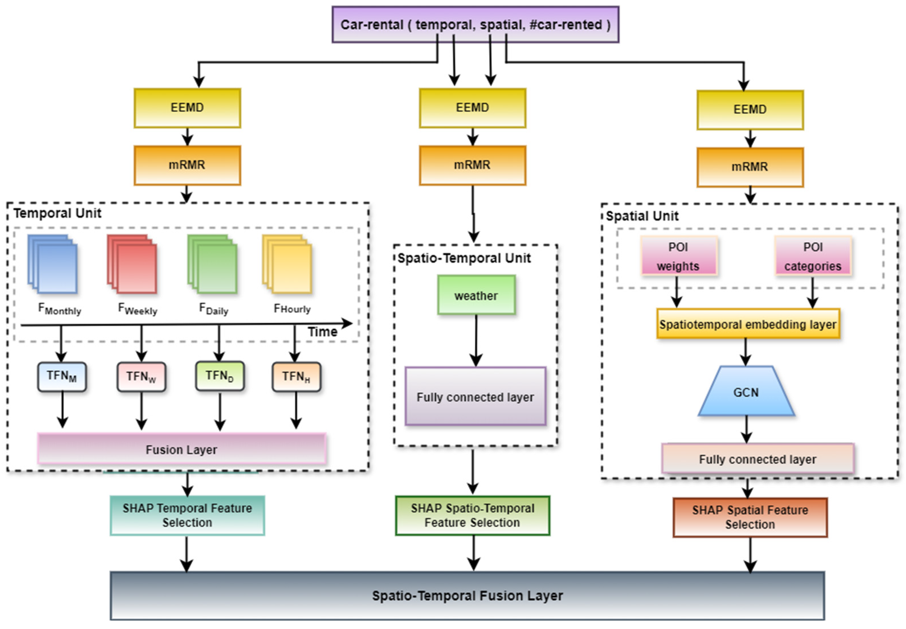
While predictive accuracy is crucial, the interpretability of predictive models has become increasingly important, particularly in high-stakes applications like urban mobility management. As deep learning models grow more complex, their lack of transparency creates challenges in understanding and interpreting model outputs, thus improving their usability in decision-making. Several explainability techniques have been explored in demand prediction. Local Interpretable Model-Agnostic Explanations (LIME), introduced by Ribeiro, Singh, and Guestrin [9], approximates black-box models using local surrogate models to provide interpretability at the individual prediction level. Studies by Nanayakkara et al. [41], Parmar et al. [42], and Shams Amiri et al. [43] have demonstrated LIME’s effectiveness in generating insights across multiple real-world applications. However, LIME has notable limitations, including sensitivity to data perturbation strategies, difficulty in defining local neighborhoods, and a reliance on simplified approximations that may not always align with the true decision boundaries of the model. A more robust alternative is Shapley Additive Explanations (SHAP), which extends from game theory to provide a theoretically grounded method for quantifying each feature’s contribution to a model’s prediction [44]. Unlike LIME, SHAP ensures consistency, fairness, and global interpretability, making it particularly suitable for high-dimensional, complex models like those used in car-sharing demand forecasting [45]. Studies have shown that SHAP offers superior explainability properties, maintaining efficiency, symmetry, and additivity, which are critical for producing reliable feature attributions [46,47]. By incorporating SHAP, eX-STIN enhances interpretability, addressing one of USTIN’s major limitations while improving predictive accuracy. This transparency allows car-sharing operators to make more informed, data-driven decisions, leading to optimized fleet distribution, reduced inefficiencies, and enhanced user satisfaction.

3. Methodology

Figure 1 illustrates the eX-STIN model, an enhanced version of the USTIN model initially described in [3]. The eX-STIN model consists of three key modules: EEMD for feature extraction, mRMR for selecting relevant and non-redundant features, and the USTIN architecture model for predictive analysis. The USTIN architecture model incorporates SHAP after each unit to enhance the understanding of feature contributions.

To further optimize predictive accuracy and interpretability, eX-STIN integrates feature reduction techniques, including feature extraction and selection, while leveraging explainable AI to provide greater transparency in model predictions. These advancements enable more reliable demand prediction and actionable insights, ultimately supporting better decision-making in car-sharing operations.

Feature extraction and selection are important parts of the eX-STIN model as they eliminate noise while preserving essential temporal, spatial, and spatio-temporal features [30,48]. The predictive model comprises three main components: a temporal unit that analyzes demand across various time scales (hourly, daily, weekly, and monthly), a spatial unit that examines POI data, and a spatio-temporal unit that models the effects of weather conditions across different locations and times [49]. Each unit employs SHAP on its output post-processing, thereby improving the model’s transparency and interpretability in the following predictive modeling phase [8].

The eX-STIN model has three types of features: temporal features ($G_t$), which show demand over time; spatial features ($G_{POI}$), which show the POIs around car-sharing stations; spatio-temporal features ($G_{ME}$), which show weather data in both time and space. We analyze these attributes via feature extraction and selection, thereafter, processing them in their respective units for final predictions.

3.1. Feature Extraction

Data analysis methodologies like EEMD reveal hidden fluctuation patterns. They effectively capture non-stationary and nonlinear features, frequently found in complex datasets [50]. EEMD decomposes $G_t$, $G_{POI}$, and $G_{ME}$ into a set of intrinsic mode functions (IMFs) and a residual component [51]. This decomposition allows a thorough analysis of the essential patterns and variations within the data.

3.1.1. Temporal Feature Extraction

The temporal feature extraction analyzes the underlying patterns in temporal data and identifies both typical and unusual demand-influenced behaviors.

$$G_t^{IMF}=\sum _{k=1}^K\left(\sum _{i=1}^N{C}_{i,k}\left(G_t\right)\right)+R\left(G_t\right)$$

(1)

where

• $C_{i,k}\left(G_t\right)$: IMFs from temporal data, with $i$ as the IMF index and $k$ as the trial index.
• $R\left(G_t\right)$: residual pattern after decomposing $G_t$.

3.1.2. Spatial Feature Extraction

The spatial feature extraction allows the accurate identification of demand hotspots by effectively defining spatial patterns that correspond significantly with high-demand regions.

$$G_{POI}^{IMF}=\sum _{k=1}^K\left(\sum _{i=1}^N{C}_{i,k}\left(G_{POI}\right)\right)+R\left(G_{POI}\right)$$

(2)

where

• $C_{i,k}\left(G_{POI}\right)$: IMFs from the spatial data.
• $R\left(G_{POI}\right)$: residual pattern left after decomposing $G_{POI}$.

3.1.3. Spatio-Temporal Feature Extraction

The spatio-temporal analysis provides important insights into how temporal events influence spatial patterns and vice versa, essential for enhancing prediction accuracy in dynamic environments.

$$G_{ME}^{IMF}=\sum _{k=1}^K\left(\sum _{i=1}^N{C}_{i,k}\left(G_{ME}\right)\right)+R\left(G_{ME}\right)$$

(3)

where

• $C_{i,k}\left(G_{ME}\right)$: IMFs from spatio-temporal data.
• $R\left(G_{ME}\right)$: residual pattern after decomposing $G_{ME}$.

3.2. Mutual Information

Entropy is a fundamental concept in information theory—first presented by Shannon as a way of measuring a random variable’s uncertainty [52]. The entropy $H\left(X\right)$ of variable $X$ is calculated as follows:

$$H\left(X\right)=-\sum _{xϵX}p\left(x\right)logp\left(x\right)$$

(4)

where

• $p\left(x\right)$: the probability mass function of $x$.

The joint entropy $H(X,Y)$ of $X$ and $Y$ is the entropy of their joint distribution:

$$H(X,Y)=-{\sum }_x{\sum }_{y}p\left(x,y\right)\mathit{log}p\left(y\right|x)$$

(5)

where

• $p(x,y)$: the joint probability mass function of $x$ and $y$.

The conditional entropy $H\left(Y|X\right)$ is the average uncertainty of $X$ given $Y$:

$$\begin{array}{}H\left(Y|X\right)=p\left(x\right)H\left(Y|X=x\right)={\displaystyle \sum _x}p\left(x\right){\displaystyle \sum _y}p\left(y|x\right)\mathit{log}p\left(y|x\right)={\sum }_x{\sum }_{y}p\left(x,y\right)\mathit{log}p\left(y\right|x)\end{array}$$

(6)

where

• $p\left(x|y\right)$: the conditional probability mass function of $x$ given $y$.

The joint entropy and the conditional entropy are related as follows:

$$H\left(X,Y\right)=H\left(X\right)+H\left(Y|X\right)$$

(7)

The mutual information $I$ is defined as follows:

$$I\left(X,Y\right)=H\left(X\right)-H\left(X|Y\right)=H\left(X\right)+H\left(Y\right)-H(X,Y)$$

(8)

3.3. Feature Selection

Following feature extraction, our model uses the mRMR method for feature selection. The mRMR method identifies the most important features, characterized by significant relevance to the target variable and low redundancy, which improves the model’s accuracy and efficiency [53]. It is also applied to the IMFs obtained from the $G_t$, $G_{POI}$, and $G_{ME}$ data through EEMD.

3.3.1. Temporal Feature Selection

The temporal feature selection process aims to find the time-related features that are most predictive while reducing the amount of redundancy in the information they offer.

$$mRMR\left(G_t^{IMF}\right)={\displaystyle \frac{1}{\left|S_t\right|}}\sum _{iϵS}I\left(F_i^t;Y\right)-{\displaystyle \frac{1}{{\left|S_t\right|}^2}}\sum _{i,jϵS}I\left(F_i^t;F_j^t\right)$$

(9)

where

• $S_t$: the subset of selected features from $G_t^{IMF}$.
• $F_i^t$: the $i\mathrm{t}\mathrm{h}$ features within the subset $S_t$.
• $I\left(F_i^t;F_j^t\right)$: the mutual information entropy between features $F_i^t$ and $F_j^t$.
• $I\left(F_i^t;Y\right)$: mutual information between feature $F_i^t$ and target variable $Y$.

3.3.2. Spatial Feature Selection

Spatial feature selection identifies key areas that affect car-sharing demand, highlighting important spatial features to improve prediction accuracy.

$$mRMR\left(G_{POI}^{IMF}\right)={\displaystyle \frac{1}{\left|S_{POI}\right|}}\sum _{iϵS}I\left(F_i^{POI};Y\right)-{\displaystyle \frac{1}{{\left|S_{POI}\right|}^2}}\sum _{i,jϵS}I\left(F_i^{POI};F_j^{POI}\right)$$

(10)

where

• $S_{POI}$: the subset of selected features from $G_{POI}^{IMF}$.
• $F_i^{POI}$: the $i\mathrm{t}\mathrm{h}$ features within the subset $S_{POI}$.
• $I\left(F_i^{POI};F_j^{POI}\right)$: the mutual information entropy between features $F_i^{POI}$ and $F_j^{POI}$.
• $I\left(F_i^{POI};Y\right)$: mutual information between feature $F_i^{POI}$ and target variable $Y$.

3.3.3. Spatio-Temporal Feature Selection

Spatio-temporal feature selection focuses on identifying the key variables that explain variations in car-sharing demand across different times and locations.

$$mRMR\left(G_{POI}^{ME}\right)={\displaystyle \frac{1}{\left|S_{ME}\right|}}\sum _{iϵS}I\left(F_i^{ME};Y\right)-{\displaystyle \frac{1}{{\left|S_{ME}\right|}^2}}\sum _{i,jϵS}I\left(F_i^{ME};F_j^{ME}\right)$$

(11)

where

• $S_{ME}$: the subset of selected features from $G_{ME}^{IMF}$.
• $F_i^{ME}$: the $i\mathrm{t}\mathrm{h}$ features within the subset $S_{ME}$.
• $I\left(F_i^{ME};F_j^{ME}\right)$: the mutual information entropy between features $F_i^{ME}$ and $F_j^{ME}$.
• $I\left(F_i^{ME};Y\right)$: mutual information between feature $F_i^{ME}$ and target variable $Y$.

The outputs of the mRMR feature selection, denoted as $F_t$, $F_{POI}$, and $F_{ME},$ are subsequently integrated into the corresponding predictive units of the model. This integration ensures that the car-sharing system’s demand predictions are both precise and reflective of the underlying spatio-temporal, spatial, and temporal patterns.

3.4. Predictive Model

This section defines the prediction model, which is an extension of our USTIN model [3]. The predictive model consists of three essential components: a temporal feature unit, a spatial feature unit, and a spatio-temporal feature unit. We apply SHAP after each unit to improve model transparency, providing interpretable insights into the influence of various features on predictions.

3.4.1. Temporal Feature Unit

The temporal feature unit processes historical demand data across various time scales (hourly, daily, weekly, and monthly). Each layer forms a Temporal Fusion Network (TFN) structure [3], which efficiently captures temporal correlations, as shown in Figure 2.

• Encoder: temporal convolutional network (TCN)

TCN serves as the encoder, processing selected temporal features $F_t$. TCN is optimized to capture long-term dependencies, a capability rooted in its hierarchical dilation structure.

$$G_t^{TCN}=ReLU \left(W_t\odot F_t+b_t\right)$$

(12)

where

• $G_t^{TCN}$: the output of the TCN.
• $W_t$: the weight matrix of the convolutional filter.
• $b_t$: the bias term.
• $\odot$: the convolution operation.

After the processing of the input sequence by the encoder, the output goes through the batch normalization before being passed to the attention mechanism. This normalization step is important for stabilizing the learning process and enhancing the model’s convergence rate.

$$G_t=\gamma \left({\displaystyle \frac{G_t^{TCN}-{\mu }_B}{\sqrt{\left({\sigma }_B^2+\epsilon \right)}}}\right)+\beta$$

(13)

where

• $G_t$: batch-normalized output at a specific time step $t$.
• ${\mu }_B,{\sigma }_B^2$: mean and variance computed over the batch.
• $\gamma ,\beta$: learnable parameters specific to each feature dimension.
• $\epsilon$: small constant added for numerical stability.

2.

Attention mechanism layer

The attention mechanism allows the incorporation of varying degrees of influence from different sequences at a given moment, which in turn affects the prediction of the sequence at the current time in time series prediction.

By employing the LSTM as a decoder, we can access the hidden layer node output $H_i$ at time $i$. This allows the model to use the state $H_i$ from the decoder’s hidden layer to compare against the hidden layer state ${\widehat{G}}_t$ at time $t$, which is derived from the encoder’s output.

$$e_{it}=a\left(H_i{G}_t\right)$$

(14)

$$a_{it}={\displaystyle \frac{exp\left(e_{it}\right)}{{\sum }_{k=1}^{T}exp\left(e_{ik}\right)}}$$

(15)

$${\widehat{G}}_i=\sum _{j=1}^T\left(a_{ij}{G}_t\right)$$

(16)

where

• $e_{it}$: the number of attentional correlations from moment $t$ to moment $i$.
• $a_{it}$: the attentional weight.
• $i$: the current time step in the decoder.
• $t$: the time steps in the encoder’s output.
• $T$: the total number of time steps in the encoder output.
• $k$: an iterator in the normalization sum.

3.

Decoder: long short-term memory layer (LSTM)

The LSTM decoder leverages the contextual information provided by the attention mechanism to enhance its sequence generation capabilities. The LSTM structure includes input gates $i_i$, forget gates $f_i$, and output gates $o_i$.

The ${\widehat{G}}_i$ obtained by the attention mechanism will be input into the next decoding layer as an input sequence, and $y_j$ will be calculated by the decoding layer:

$$i_i=\sigma (W_i.\left[H_{i-1} y_{i-1} {\widehat{G}}_i\right]+b_i)$$

(17)

$$f_i=\sigma (W_f.\left[H_{i-1} y_{i-1} {\widehat{G}}_i\right]+b_f)$$

(18)

$$o_i=\sigma (W_o.\left[H_{i-1} y_{i-1} {\widehat{G}}_i\right]+b_o)$$

(19)

$$g_i=tanh(W_g\left[H_{i-1} y_{i-1} {\widehat{G}}_i\right]+b_g)$$

(20)

$$c_i=i_i\odot g_i+f_i\odot c_{i-1}$$

(21)

$$H_i=o_i\odot tanh\left(c_i\right)$$

(22)

where

• $W_i, W_f, W_o, and W_g$: weight matrices for input gate, forget gate, output gate, and candidate cell state, respectively.
• $b_i,$ $b_f, b_o, and b_g:$ bias terms for input gate, forget gate, output gate, and candidate cell state, respectively.
• $c_i$: the current cell state.
• $c_{i-1}$: the cell state from the previous time step.
• $H_i$: the current hidden state.
• $\sigma$: sigmoid activation function.
• $\odot :$ element-wise multiplication.

To effectively combine the outputs from the four LSTM decoders associated with different time scales (daily, weekly, monthly, and yearly), we use a fully connected layer. This method enhances the model’s ability to capture complex interdependencies among the data.

$$X_{sp}=ReLU(W_{sp}.\left[H_p+H_D+H_W+H_M\right]+b_{sp}$$

(23)

where

• $H_p,H_D, H_W, and H_M$: represents the concatenated outputs from the LSTM decoders at four different time scales (daily, weekly, monthly, and yearly).
• $W_{sp}$: the weight matrix of the fully connected layer.
• $b_{sp}$: the bias of the dense fully connected layer.

3.4.2. Spatial Feature Unit

A spatial unit architecture has been implemented to efficiently handle POI features, which includes the following:

• Spatial density calculation

POI density around each parking station represents the concentration of various POIs, considering both the number of POIs and their spatial distance within a radius $R$.

The distance between a station $S_i$ and a ${POI}_{j }$ is calculated using the Haversine formula:

$$d\left(S_i,{POI}_j\right)=2.r arcsin\sqrt{{\mathit{sin}}^2\left({\displaystyle \frac{∆{lat}_{ij}}{2}}\right)+\mathit{cos}\left({lat}_i\right)·\mathit{cos}\left({lat}_j\right)·{\mathit{sin}}^2\left({\displaystyle \frac{∆{lon}_{ij}}{2}}\right)}$$

(24)

where $r$ is the Earth’s radius, and $∆{lat}_{ij}$ and $∆{lon}_{ij}$ are the differences in latitude and longitude between stations $S_i$ and ${POI}_{j }$, respectively.

The density of each POI ($D_{{POI}_j}$) is formulated as follows:

$$D_{{POI}_j}=\left\{\begin{array}{c}1ifd\left(S_i,{POI}_j\right) \le 1\\ 0otherwise\end{array}\right.$$

(25)

2.

Regression model

The variance in car sharing is much bigger than its mean, indicating an overdispersion problem, which necessitates the use of the negative binomial distribution for parameter estimation [54]. The regression model comprises an intercept term (${\beta }_0)$, regression coefficients $({\beta }_1,\dots , {\beta }_n)$ for each variable, and an error term ($\epsilon$). The order quantity at each car-sharing station is represented as $\left(u_i\right)$, while the densities of other POI categories are shown as $(x_1,\dots , x_n).$ We employ Maximum Likelihood Estimation (MLE) to estimate these coefficients while upholding a significance level of 5%. The regression equation is expressed as follows:

$$\mathit{ln}\left(u_i\right)={\beta }_0+{\beta }_1·x_1+{\beta }_2·x_2+\dots +{\beta }_n·x_n+\epsilon$$

(26)

3.

Spatio-temporal embedding layer

The selected features $F_{POI}$ and the corresponding weights vector $W_{POI}$, which contain coefficients used in Equation (26), are input into a spatio-temporal embedding layer:

$$E_{POI}=ReLU \left(W_{POI}·F_{POI}\right)$$

(27)

4.

Graph convolutional network layer (GCN)

The output of the spatio-temporal embedding layer is fed into a GCN layer. This layer employs the mean aggregation function to capture spatial relationships among POIs:

$$H_{POI}^n=\left({\displaystyle \frac{1}{D_{POI}}}\right)AGG{·E}_{POI}·A_{POI}$$

(28)

5.

Fully connected layer

This unit uses a fully connected layer to facilitate the model’s accurate demand predictions.

$$X_{MC}=ReLU (W_{MC}·H_{POI}^n+b_{MC})$$

(29)

where

• $W_{MC}$: weight of the fully connected layer.
• $b_{MC}$: bias of the fully connected layer.

3.4.3. Spatio-Temporal Feature Unit

For the selected meteorological features $F_{ME}$, we employed a fully connected layer neural network architecture to model the effects of weather conditions across time and space.

$$X_{ME}=ReLU (W_{ME}·F_{ME}+b_{ME})$$

(30)

where

• $W_{ME}$: weight of the fully connected layer.
• $b_{ME}$: bias of the fully connected layer.

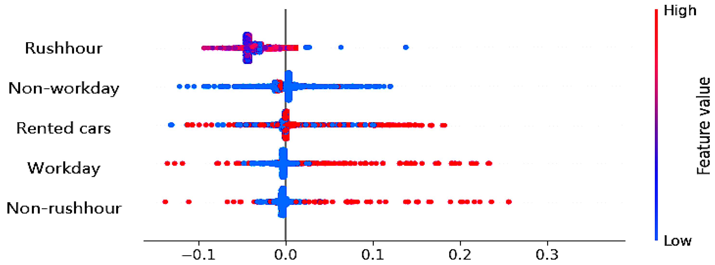
3.4.4. Shapley Additive Explanation Analysis and Model Training

For interpretability, we leverage SHAP due to its model-agnostic framework that provides consistent and interpretable explanations across various model types within the system [55]. SHAP guarantees consistency when comparing feature contributions, making it much easier to look at the stages of our predictive model [56]. Moreover, SHAP emerges as the most advantageous option when it comes to computational performance [57]. Each unit’s output undergoes SHAP analysis—offering clear insights into how different features influence predictions. Before these SHAP outputs from the temporal, spatial, and spatio-temporal units are integrated, they are normalized to align their scales and dimensions.

$$X_{ex}={W_{Sp}\otimes X_{sp}^{SHAP}+W}_{Mc}\otimes X_{Mc}^{SHAP}+W_{ME}\otimes X_{ME}^{SHAP}+b_{ex}$$

(31)

The model utilizes back-propagation with the Adam optimizer for the efficient training and improvement of predictive accuracy. The prediction results of car demand ${\tilde{X}}_{tk}$ are obtained by Equation (30).

$${\tilde{X}}_{tk}=W_{ex}\otimes X_{ex}+b_{tk}$$

(32)

where

• $X_{sp}^{SHAP}$: the normalized SHAP output from the temporal feature unit.
• $X_{Mc}^{SHAP}$: the normalized SHAP output from the spatial feature unit.
• $X_{ME}^{SHAP}$: the normalized SHAP output from the spatio-temporal feature unit.
• $W_{Sp}$, $W_{Mc}$, and $W_{ME}$: the weight matrices.
• $b_{ex}$: the bias.
• $W_{ex}$: the weight matrix that maps the final integrated feature representation to the predicted car demand.

4. Experimental Section

This section presents a comprehensive experimental framework designed to ensure a transparent and reproducible evaluation of the proposed eX-STIN model. Section 4.1 provides an overview of the dataset used in this study, followed by the experimental settings, including data preprocessing and training configuration, in Section 4.2. Section 4.3 introduces the baseline models used for comparison. Section 4.4 and Section 4.5 detail the model configuration and performance evaluation criteria [2], establishing the basis for a rigorous assessment of predictive accuracy and interpretability.

4.1. Data Description

The dataset utilized in this study consists of over 1 million records of car-sharing usage across 860 parking lots in Chongqing. To enrich the model’s predictive capabilities, meteorological and point-of-interest (POI) data were collected through web crawling [2], ensuring a comprehensive representation of influential factors. Given the presence of noise, outliers, missing values, and irrelevant features, a pre-processing pipeline was implemented. This included K-nearest neighbor (KNN) imputation to address missing values and min–max normalization to scale numerical features between 0 and 1, thereby enhancing data consistency and optimizing model performance [2,58].

Table 1. Influencing indicator system of the potential demand for car sharing.

First-Level Indicator	Second-Level Indicator
Usage feature	rented cars
Temporal features	workday (1 for yes and 0 for no); rush hour (1 for yes and 0 for no)
Weather conditions	temperature (°C), precipitation (1 for yes and 0 for no), and AQI (Air Quality Index)
Building land attribute	hotel, shopping, domestic services, beauty, tourist attractions, leisure and entertainment, work out, education and training, culture media, medical, car services, transportation facilities, finance, real estate, corporate, government agency, entrance and exit, natural features, administrative landmark, and door address

presents the factors that influence the future demand for car sharing.

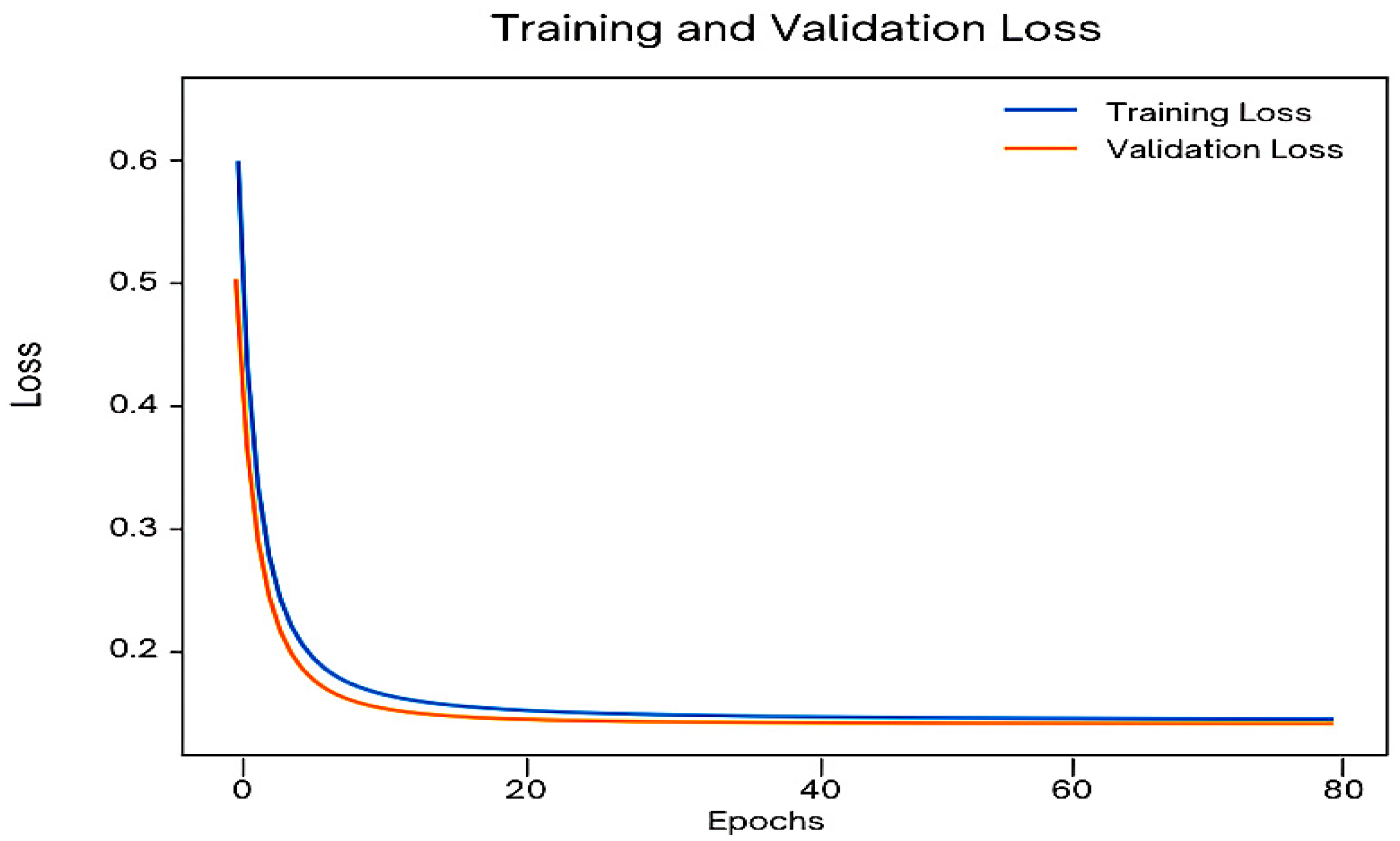
4.2. Experimental Setting

We used TensorFlow 1.14.0, Keras 2.2.4-tf, Pandas 0.23.4, Sklearn 0.21.1, Numpy 1.18.1, Matplotlib 3.1.0, and Statsmodels 0.10.1 [2].

The models were implemented using a PC with an i7 Intel (R) Core™i7-7500U CPU running at 3.00 GHz and 8 GB RAM with the Windows 10 operating system under the Python 3.7 development environment [59].

4.3. Baseline Models’ Configuration

We used a k-fold cross-validation technique with k = 5 and grid search to minimize overfitting by pinpointing the optimal hyperparameters of the baseline models.

Table 2. Baseline models’ configuration.

Model	Hyperparameters
MLP	2 fully connected layers, 20 and 15 hidden units
XGBoost	N_estimators: 25 Max_depth: 5
KNN	N_neighbours: 5 Weights: “uniform”
RF	N_estimators: 100 Max_depth: 5 Min_samples_split: 15
LSTM	Hidden layers: 2 Hidden units: 25, 15 neurons Learning rate: 0.01 Drop out: 0.5 Optimizer: Adam Epochs: 80
CNN-LSTM	CNN layers: 2 LSTM layers: 2 Filters: 64 Kernel size: 3 LSTM units: 50 Dropout: 0.3 Optimizer: Adam
Att-LSTM	Layers: 5 Units: 50 Attention type: Bahdanau Dropout: 0.4 Optimizer: Adam
ConvLSTM	Layers: 2 Filters: 64 Kernel size: 3 × 3 Dropout: 0.3 Optimizer: Adam
GATs	Number of attention heads: 4 Hidden units: 20 Learning rate: 0.01 Dropout: 0.6 Optimizer: Adam
Transformer	Heads: 4 Layers: 3 Size: 128 Feedforward size: 512 Dropout: 0.1 Optimizer: Adam
ST-GCN	Spatial graph convolutional layers: 3 Hidden units: 64 Kernel size: 5 Dropout: 0.2 Optimizer: Adam
DCN	Cross layers: 3 Deep layers: 2 Hidden units deep layer: 32 Dropout: 0.2 Optimizer: Adam

outlines the configurations for each baseline model:

4.4. Model Configuration

In our proposed eX-STIN model, we utilized k-fold cross-validation with k = 5 and grid search to fine-tune the hyperparameters, mitigate overfitting, and identify the most optimal hyperparameters [60].

Table 3. eX-STIN model configuration.

Model	Hyperparameters
TCN	Hidden layers: 3 Kernel size: 3 Dilations: [1, 2, 4, 8, 16, 32, 64] Number filters: 64 Learning rate: 0.01 Drop out: 0.2 Optimizer: Adam Epochs: 80
LSTM	Hidden layers: 2 Hidden units: 25, 15 neurons Learning rate: 0.01 Drop out: 0.3 Optimizer: Adam Epochs: 100
GCN	Hidden layers: 2 (32, 64 neurons) Hidden units: 32, 64 neurons Learning rate: 0.01 Epochs: 80

summarizes the eX-STIN model configuration:

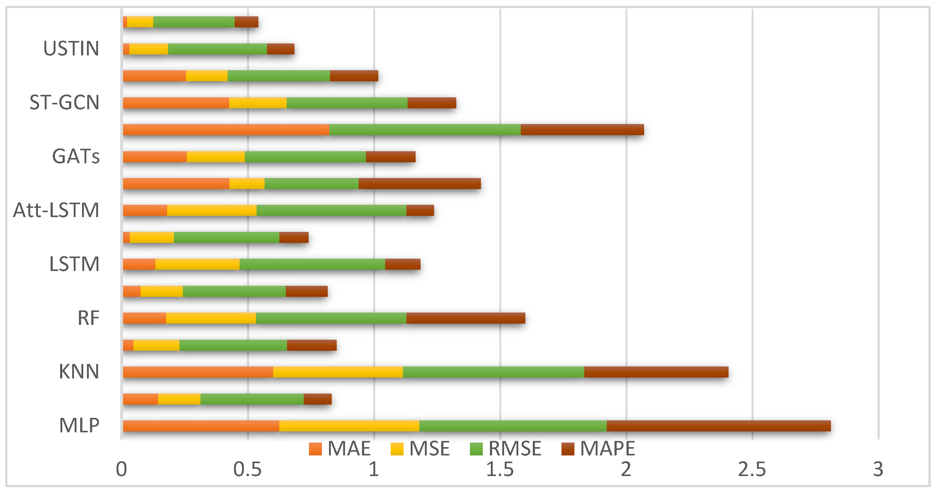
4.5. Evaluation Metrics

Evaluation metrics assess the accuracy of predictions against actual historical data, enabling comparisons across different predictive models using the same dataset [61].

4.5.1. Mean Absolute Error (MAE)

MAE represents the average of absolute prediction errors.

$$MAE=mean \left(absolute \left({expected}_{value}-{predicted}_{value}\right)\right)$$

(33)

4.5.2. Mean Square Error (MSE)

MSE measures the mean of the squared prediction errors, emphasizing larger errors.

$$MSE=mean\left({\left({expected}_{value}-{predicted}_{value}\right)}^2\right)$$

(34)

4.5.3. Root Mean Square Error (RMSE)

RMSE imposes a greater penalty on significant prediction errors compared to Mean Absolute Error (MAE).

$$RMSE=sqrt \left(MSE\right)$$

(35)

4.5.4. Mean Absolute Percentage Error (MAPE)

MAPE is a commonly utilized metric for evaluating the accuracy of forecasts. It can be defined using the following formula:

$$MAPE={\displaystyle \frac{100}{n}}\sum _{t=1}^n\left|{\displaystyle \frac{A_t-F_t}{A_t}}\right|$$

(36)

where

• $A_t$: the actual value.
• $F_t$: the forecast value.
• $n$: the number of fitted points.

5. Discussion

5.1. Evaluation of eX-STIN for Car-Sharing Demand Prediction

This study aims to develop an explainable predictive model for car demand prediction, designed to assist operators in making informed decisions that enhance the efficiency and user experience of their services. To evaluate the proposed eX-STIN model, we compared it against several baseline models using performance metrics such as MAE, MSE, RMSE, and MAPE.

Table 4. Evaluation results.

	MAE	MSE	RMSE	MAPE
MLP	0.626	0.554	0.744	0.887
TCN	0.145	0.168	0.410	0.109
KNN	0.601	0.515	0.718	0.571
GCN	0.048	0.182	0.427	0.195
RF	0.177	0.356	0.597	0.469
XGBoost	0.076	0.167	0.409	0.164
LSTM	0.135	0.333	0.577	0.139
CNN-LSTM	0.033	0.175	0.418	0.115
Att-LSTM	0.181	0.354	0.595	0.108
ConvLSTM	0.428	0.139	0.373	0.484
GATs	0.259	0.230	0.480	0.195
Transformer	0.824	0. 575	0.758	0.488
ST-GCN	0.426	0.229	0.479	0.192
DCN	0.255	0.165	0.406	0.191
USTIN	0.031	0.154	0.392	0.108
Our(eX-STIN)	0.022	0.104	0.322	0.094

presents the comparison results, with the smallest errors highlighted in bold to indicate the best-performing model for each metric.

The eX-STIN model exhibits significant advantages compared to other baseline models, indicating considerable improvements across different metrics. In comparison to the MLP model, the eX-STIN model attained reductions of 96.49% in MAE, 81.23% in MSE, 56.72% in RMSE, and 89.40% in MAPE. In comparison to the TCN model, the eX-STIN model demonstrated enhancements of 84.83% in MAE, 38.10% in MSE, 21.46% in RMSE, and 13.76% in MAPE.

Further comparisons revealed that the eX-STIN model outperformed the KNN model, with improvements of 96.34% in MAE, 79.81% in MSE, 55.15% in RMSE, and 83.54% in MAPE. When compared to the GCN model, the eX-STIN model showed improvements of 54.17% in MAE, 42.86% in MSE, 24.59% in RMSE, and 51.79% in MAPE. In comparison with the RF model, eX-STIN demonstrated enhancements of 87.57% in MAE, 70.79% in MSE, 46.06% in RMSE, and 79.96% in MAPE. Finally, a comparison with the XGBoost model revealed improvements of 71.05% in MAE, 37.72% in MSE, 21.27% in RMSE, and 42.68% in MAPE.

Additionally, in comparison to more intricate models—such as Att-LSTM, ConvLSTM, GATs, Transformer, ST-GCN, and DCN—the eX-STIN model consistently exhibited significant enhancements across all the metrics. Compared to Att-LSTM, eX-STIN showed enhancements of 87.85% in MAE, 70.62% in MSE, 45.88% in RMSE, and 13.00% in MAPE. The improvements for ConvLSTM were 94.86% in MAE, 25.18% in MSE, 13.67% in RMSE, and 80.58% in MAPE. Concerning GATs, eX-STIN showed enhancements of 91.51% in MAE, 54.78% in MSE, 32.92% in RMSE, and 51.79% in MAPE. eX-STIN significantly outperformed the transformer model, achieving improvements of 97.33% in MAE, 81.91% in MSE, 57.52% in RMSE, and 80.74% in MAPE. In comparison to ST-GCN, the improvements were 94.84% in MAE, 54.59% in MSE, 32.77% in RMSE, and 51.04% in MAPE. Finally, compared to DCN, eX-STIN demonstrated enhancements of 91.37% in MAE, 36.97% in MSE, 20.69% in RMSE, and 50.79% in MAPE. Compared to our previously proposed USTIN model, eX-STIN achieved reductions of 29.03% in MAE, 32.47% in MSE, 17.86% in RMSE, and 12.96% in MAPE.

These results clearly validate the effectiveness of the proposed model, confirming that the research objectives were successfully met. The eX-STIN model achieves superior predictive accuracy, contributing to the advancement of spatio-temporal modeling techniques for car-sharing demand prediction in urban mobility research.

Figure 3 compares prediction errors across models, showing that eX-STIN achieves the lowest evaluation metrics, outperforming both traditional and deep learning models. While CNN-LSTM, TCN, GCN, and ST-GCN demonstrate relatively strong performance, they remain less effective than eX-STIN. USTIN was selected as the principal benchmark for comparison, as it forms the architectural foundation of the proposed eX-STIN model. Unlike other models, which differ significantly in design and modeling objectives, USTIN integrates spatio-temporal inference through specialized feature units. This structural alignment makes it the most appropriate baseline for evaluating the effectiveness of the enhancements introduced in eX-STIN, including advanced feature extraction and interpretability mechanisms.

5.2. Prediction Results and Interpretability Analysis

The training and validation loss curves of the eX-STIN model, as illustrated in Figure 4, demonstrate its ability to learn effectively from the data while avoiding overfitting. Figure 5 further illustrates the model’s accuracy in predicting car-sharing demand by comparing actual and predicted values across various parking lots. The close alignment between predicted and actual values highlights the model’s precision, which is essential for supporting efficient decision-making in car-sharing operations. Compared to traditional machine learning approaches such as MLP, KNN, and RF, the eX-STIN model consistently achieves lower error rates across all evaluation metrics. In addition, it outperforms advanced deep learning architectures including CNN-LSTM, Transformer, and ST-GCN, indicating the effectiveness of its design.

The strong performance of eX-STIN results from the integration of advanced feature reduction and interpretability methods. Specifically, it employs EEMD to analyze complex temporal, spatial, and spatio-temporal dependencies in car-sharing data, effectively capturing patterns that traditional methods often fail to detect. Additionally, it utilizes mRMR to refine the feature set by selecting only the most relevant predictors, optimizing model performance while preserving predictive accuracy. Dashdorj et al. [62] emphasized that such feature reduction techniques enhance deep learning models by improving accuracy and computational efficiency, particularly in large-scale applications. Similarly, Troiano et al. [63] highlighted the benefits of compressing high-dimensional input into more informative representations, contributing to improved model outcomes. These findings support the integration of EEMD and mRMR in eX-STIN, as they contribute to a more focused and efficient learning process while reducing the risk of overfitting.

Alongside its feature reduction method, eX-STIN incorporates SHAP to enhance interpretability by measuring the contribution of each input feature to the model’s predictions. The significance of explainable artificial intelligence is well documented in the literature. Marey et al. [64] demonstrated that the integration of SHAP with deep learning models improves transparency and predictive accuracy in financial applications. Khan and Park [65] showed that combining CNNs with LIME and Grad-CAM enhances prediction accuracy and interpretability in traffic sign recognition systems. These findings underscore the importance of embedding explainability into deep learning models for urban mobility prediction.

Building upon the USTIN architecture, the eX-STIN model is structured into three units. The temporal feature unit focuses on predicting short-term car demand trends, the spatial feature unit assesses the influence of points of interest on demand to identify service hotspots, and the spatio-temporal feature unit adjusts predictions based on environmental variations that affect demand patterns. Although USTIN demonstrates strong capabilities in modeling spatio-temporal interdependencies, eX-STIN consistently surpasses it across all evaluation metrics. This improvement highlights the added value of EEMD and mRMR, which enable the model to extract relevant features while eliminating redundant inputs, thereby enhancing generalization and robustness.

However, the eX-STIN model presents certain limitations. It relies exclusively on temporal, spatial, and spatio-temporal features and does not incorporate direct user input such as customer preferences, travel intentions, or real-time behavioral feedback. This constraint may limit its ability to capture abrupt shifts in user demand driven by external factors, emerging patterns, or behavioral change, which are often critical for dynamic mobility services. Incorporating user-oriented contextual data could further improve adaptability and responsiveness in future iterations of the model.

The results of this study indicate that eX-STIN outperforms existing models while aligning with current priorities in predictive modeling research, where both accuracy and interpretability are critical objectives.

5.3. Features Impact on the Unit’s Output

5.3.1. Temporal Unit

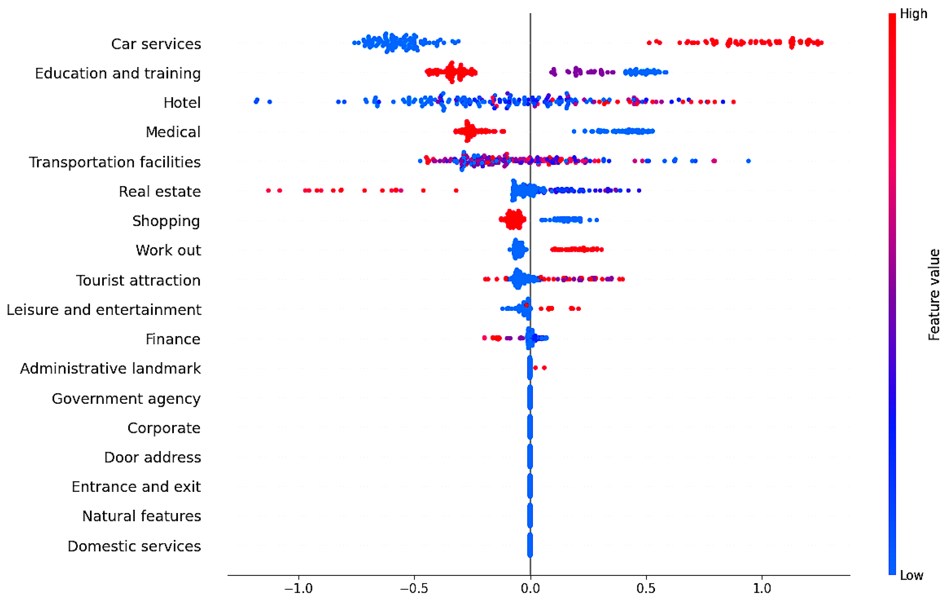
Figure 6 provides valuable insights into the impact of different temporal features on the temporal unit’s output. The findings indicate a strong negative impact of rush hour conditions, shown by red dots clustering to the left of the zero line. This suggests that high traffic congestion significantly affects car-sharing usage. Conversely, positive impacts are evident for features like rented cars, workdays, and non-rush hour periods, with red dots mostly located on the right side of the zero line. This indicates that periods of lower congestion and routine commuting times are more favorable for car sharing, likely due to predictable user behavior and faster travel times.

5.3.2. Spatial Unit

Figure 7 offers an important insight into the influence of various spatial features on the model’s output. It shows that features like car services, hotels, workout facilities, and tourist attractions are mostly located on the right side of the zero line, indicating a positive impact on the model’s predictions. These locations attract frequent and often short-term visitors who benefit from the flexibility of car sharing. Conversely, features associated with education and training, medical facilities, transportation hubs, shopping centers, and finance-related areas mostly appear with red dots on the left side of the zero line, suggesting a negative impact on car-sharing usage. This negative impact may come from high congestion levels, limited parking availability, and the presence of alternative transportation modes, which are often more accessible and cost-efficient for daily travelers. Meanwhile, administrative landmarks, government agencies, corporate addresses, entrances and exits, natural features, and domestic services show a neutral impact, with dots clustered around the center. These areas may not generate significant fluctuations in car-sharing demand, as they may not be primary destinations for car-sharing users.

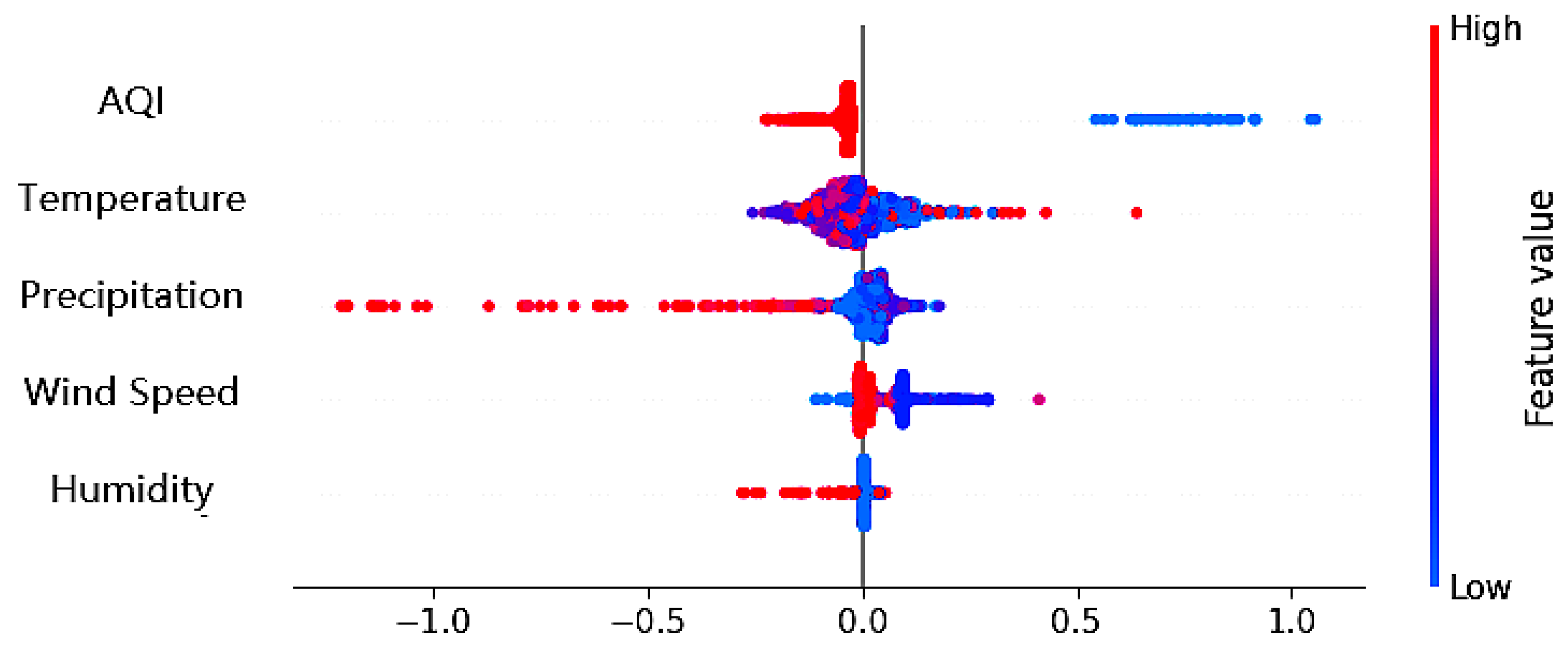
5.3.3. Spatio-Temporal Unit

Figure 8 illustrates the patterns in which meteorological variables affect the spatio-temporal unit’s output. Poor air quality, indicated by high AQI values, negatively affects car demand predictions, with red dots predominantly clustered on the left side of the zero line. Conversely, low AQI levels, signifying favorable air quality, generally exert a positive effect. Variables such as temperature, precipitation, wind speed, and humidity show varying impacts, encompassing both positive and negative effects. Higher levels of precipitation and humidity frequently result in negative impacts, whereas the implications of temperature and wind speed tend to be less predictable.

6. Conclusions

Our research introduces the Explainable Spatio-Temporal Inference Network (eX-STIN), a novel model that improves both the accuracy and interpretability of car-sharing demand predictions. Built upon the core foundation of its predecessor, the Unified Spatio-Temporal Inference Network (USTIN), eX-STIN expands the predictive framework by incorporating feature extraction, feature selection, and interpretability mechanisms. The model employs Ensemble Empirical Mode Decomposition (EEMD) for feature extraction, significantly reducing data dimensionality and improving computational performance. Following this, the Minimum Redundancy Maximum Relevance (mRMR) method is utilized for feature selection, ensuring that only pertinent and non-redundant features are retained, which decreases the probability of overfitting.

Unlike traditional deep learning models, which often operate as black-box systems, eX-STIN enhances transparency by utilizing SHAP (Shapley Additive Explanations) to explain the contribution of each feature to the model’s predictions. This interpretability mechanism provides clear insights into how specific factors influence car demand predictions, enabling data-driven decision-making that supports more strategic resource allocation and operational optimization in car-sharing services.

Furthermore, eX-STIN builds upon the predictive framework of its predecessor by incorporating specialized temporal, spatial, and spatio-temporal units. The temporal unit captures demand patterns across various time scales, the spatial unit identifies high-demand areas using points of interest, and the spatio-temporal unit models the impact of weather conditions on demand across different times and locations. By integrating these factors into interpretable modules, eX-STIN enhances its ability to deliver actionable insights for urban transportation planning, offering a deeper understanding of the key factors driving demand. These insights are essential for optimizing resource allocation, improving operational strategies, and ensuring the more efficient management of transportation systems.

Experiments on real-world datasets validate the effectiveness of the eX-STIN model, which not only outperforms state-of-the-art models and its predecessor but also provides valuable insights into the impact of various features on future car demands. Initially developed to predict car usage across various parking lots, our approach has potential applications in other fields where temporal, spatial, and spatio-temporal dynamics are critical. However, the eX-STIN model has limitations; it relies exclusively on temporal, spatial, and spatio-temporal data and does not incorporate direct user input, such as customer preferences or real-time feedback, potentially overlooking behavioral changes that influence demand. Future research will focus on integrating real-time data sources to improve adaptability and responsiveness. Enhancing the model’s ability to process diverse urban datasets and incorporating adaptive learning techniques will further optimize demand predictions for evolving transportation systems.

References

1. Qian, X.; Guo, S.; Aggarwal, V. DROP: Deep relocating option policy for optimal ride-hailing vehicle repositioning. Transp. Res. Part C Emerg. Technol. 2022, 145, 103923. [Google Scholar] [CrossRef]
2. Brahimi, N.; Zhang, H.; Dai, L.; Zhang, J.; Benito, R.M. Modelling on Car-Sharing Serial Prediction Based on Machine Learning and Deep Learning. Complexity 2022, 2022, 8843000. [Google Scholar] [CrossRef]
3. Brahimi, N.; Zhang, H.; Zaidi, S.D.A.; Dai, L. A Unified Spatio-Temporal Inference Network for Car-Sharing Serial Prediction. Sensors 2024, 24, 1266. [Google Scholar] [CrossRef] [PubMed]
4. Ke, J.; Zheng, H.; Yang, H.; Chen, X. (Michael) Short-term forecasting of passenger demand under on-demand ride services: A spatio-temporal deep learning approach. Transp. Res. Part C Emerg. Technol. 2017, 85, 591–608. [Google Scholar] [CrossRef]
5. Ströhle, P.; Flath, C.M.; Gärttner, J. Leveraging Customer Flexibility for Car-Sharing Fleet Optimization. Transp. Sci. 2018, 53, 42–61. [Google Scholar] [CrossRef]
6. Moein, E.; Awasthi, A. Carsharing customer demand forecasting using causal, time series and neural network methods: A case study. Int. J. Serv. Oper. Manag. 2020, 35, 36–57. [Google Scholar] [CrossRef]
7. Wang, H.; Yuan, Y.; Yang, X.T.; Zhao, T.; Liu, Y. Deep Q learning-based traffic signal control algorithms: Model development and evaluation with field data. J. Intell. Transp. Syst. 2023, 27, 314–334. [Google Scholar] [CrossRef]
8. Lundberg, S.M.; Allen, P.G.; Lee, S.-I. A Unified Approach to Interpreting Model Predictions. Adv. Neural Inf. Process. Syst. 2017, 30. Available online: https://github.com/slundberg/shap (accessed on 25 April 2024).
9. Ribeiro, M.T.; Singh, S.; Guestrin, C. “Why should i trust you?” Explaining the predictions of any classifier. In Proceedings of the 22nd ACM SIGKDD International Conference on Knowledge Discovery and Data Mining, San Francisco, CA, USA, 13–17 August 2016; pp. 1135–1144. [Google Scholar] [CrossRef]
10. Samek, W.; Montavon, G.; Vedaldi, A.; Hansen, L.K.; Müller, K.-R. Explainable AI: Interpreting, Explaining and Visualizing Deep Learning; Springer: Berlin, Germany, 2019; Volume 11700. [Google Scholar] [CrossRef]
11. Chandrashekar, G.; Sahin, F. A survey on feature selection methods. Comput. Electr. Eng. 2014, 40, 16–28. [Google Scholar] [CrossRef]
12. Wang, S.; Cao, J.; Yu, P.S. Deep Learning for Spatio-Temporal Data Mining: A Survey. IEEE Trans. Knowl. Data Eng. 2022, 34, 3681–3700. [Google Scholar] [CrossRef]
13. Firnkorn, J.; Müller, M. Selling Mobility instead of Cars: New Business Strategies of Automakers and the Impact on Private Vehicle Holding. Bus. Strateg. Environ. 2012, 21, 264–280. [Google Scholar] [CrossRef]
14. Becker, H.; Ciari, F.; Axhausen, K.W. Comparing car-sharing schemes in Switzerland: User groups and usage patterns. Transp. Res. Part A Policy Pract. 2017, 97, 17–29. [Google Scholar] [CrossRef]
15. Nair, R.; Miller-Hooks, E. Fleet Management for Vehicle Sharing Operations. Transp. Sci. 2010, 45, 524–540. [Google Scholar] [CrossRef]
16. Müller, J.; Homem de Almeida Correia, G.; Bogenberger, K. An explanatory model approach for the spatial distribution of free-floating carsharing bookings: A case-study of German cities. Sustainability 2017, 9, 1290. [Google Scholar] [CrossRef]
17. Cheng, Y. Optimizing Location of Car-Sharing Stations Based on Potential Travel Demand and Present Operation Characteristics: The Case of Chengdu. J. Adv. Transp. 2019, 2019, 7546303. [Google Scholar] [CrossRef]
18. Boyaci, B.; Zografos, K.G.; Geroliminis, N. An optimization framework for the development of efficient one-way car-sharing systems. Eur. J. Oper. Res. 2015, 240, 718–733. [Google Scholar] [CrossRef]
19. Hua, Y.; Zhao, D.; Wang, X.; Li, X. Joint infrastructure planning and fleet management for one-way electric car sharing under time-varying uncertain demand. Transp. Res. Part B Methodol. 2019, 128, 185–206. [Google Scholar] [CrossRef]
20. Deza, A.; Huang, K.; Metel, M.R. Charging station optimization for balanced electric car sharing. Discret. Appl. Math. 2022, 308, 187–197. [Google Scholar] [CrossRef]
21. Atter, G.B.; Leitner, M.; Ljubi, I. Location of Charging Stations in Electric Car Sharing Systems. Transp. Sci. 2020, 54, 1408–1438. [Google Scholar] [CrossRef]
22. Kuwahara, M.; Yoshioka, A.; Uno, N. Practical Searching Optimal One-Way Carsharing Stations to Be Equipped with Additional Chargers for Preventing Opportunity Loss Caused by Low SoC. Int. J. Intell. Transp. Syst. Res. 2021, 19, 12–21. [Google Scholar] [CrossRef]
23. Lu, X.; Zhang, Q.; Peng, Z.; Shao, Z.; Song, H.; Wang, W. Charging and relocating optimization for electric vehicle car-sharing: An event-based strategy improvement approach. Energy 2020, 207, 118285. [Google Scholar] [CrossRef]
24. Alencar, V.A.; Rooke, F.; Cocca, M.; Vassio, L.; Almeida, J.; Vieira, A.B. Characterizing client usage patterns and service demand for car-sharing systems. Inf. Syst. 2021, 98, 101448. [Google Scholar] [CrossRef]
25. Hu, S.; Chen, P.; Lin, H.; Xie, C.; Chen, X. Promoting carsharing attractiveness and efficiency: An exploratory analysis. Transp. Res. Part D Transp. Environ. 2018, 65, 229–243. [Google Scholar] [CrossRef]
26. Di Febbraro, A.; Sacco, N.; Saeednia, M. One-Way Car-Sharing Profit Maximization by Means of User-Based Vehicle Relocation. IEEE Trans. Intell. Transp. Syst. 2019, 20, 628–641. [Google Scholar] [CrossRef]
27. Deveci, M.; Canıtez, F.; Gökaşar, I. WASPAS and TOPSIS based interval type-2 fuzzy MCDM method for a selection of a car sharing station. Sustain. Cities Soc. 2018, 41, 777–791. [Google Scholar] [CrossRef]
28. Zhao, L.; Zhou, Y.; Lu, H.; Fujita, H. Parallel computing method of deep belief networks and its application to traffic flow prediction. Knowl.-Based Syst. 2019, 163, 972–987. [Google Scholar] [CrossRef]
29. Huang, N.E.; Wu, M.L.; Qu, W.; Long, S.R.; Shen, S.S.P. Applications of Hilbert-Huang transform to non-stationary financial time series analysis. Appl. Stoch. Model. Bus. Ind. 2003, 19, 245–268. [Google Scholar] [CrossRef]
30. Huang, N.E.; Shen, Z.; Long, S.R.; Wu, M.C.; Snin, H.H.; Zheng, Q.; Yen, N.C.; Tung, C.C.; Liu, H.H. The empirical mode decomposition and the Hubert spectrum for nonlinear and non-stationary time series analysis. Proc. R. Soc. A Math. Phys. Eng. Sci. 1998, 454, 903–995. [Google Scholar] [CrossRef]
31. Hamad, K.; Shourijeh, M.T.; Lee, E.; Faghri, A. Near-term travel speed prediction utilizing Hilbert-Huang transform. Comput.-Aided Civ. Infrastruct. Eng. 2009, 24, 551–576. [Google Scholar] [CrossRef]
32. Wei, Y.; Chen, M.C. Forecasting the short-term metro passenger flow with empirical mode decomposition and neural networks. Transp. Res. Part C Emerg. Technol. 2012, 21, 148–162. [Google Scholar] [CrossRef]
33. Sun, W.; Ren, C. Short-term prediction of carbon emissions based on the EEMD-PSOBP model. Environ. Sci. Pollut. Res. 2021, 28, 56580–56594. [Google Scholar] [CrossRef] [PubMed]
34. Sun, W.; Xu, C. Carbon price prediction based on modified wavelet least square support vector machine. Sci. Total Environ. 2021, 754, 142052. [Google Scholar] [CrossRef] [PubMed]
35. Li, J.; Deng, D.; Zhao, J.; Cai, D.; Hu, W.; Zhang, M.; Huang, Q. A Novel Hybrid Short-Term Load Forecasting Method of Smart Grid Using MLR and LSTM Neural Network. IEEE Trans. Ind. Inform. 2021, 17, 2443–2452. [Google Scholar] [CrossRef]
36. Pandey, P.; Bokde, N.D.; Dongre, S.; Gupta, R. Hybrid Models for Water Demand Forecasting. J. Water Resour. Plan. Manag. 2020, 147, 04020106. [Google Scholar] [CrossRef]
37. Gu, X.; Guo, J.; Xiao, L.; Ming, T.; Li, C. A Feature Selection Algorithm Based on Equal Interval Division and Minimal-Redundancy–Maximal-Relevance. Neural Process. Lett. 2020, 51, 1237–1263. [Google Scholar] [CrossRef]
38. Gu, X.; Guo, J.; Xiao, L.; Li, C. Conditional mutual information-based feature selection algorithm for maximal relevance minimal redundancy. Appl. Intell. 2021, 52, 1436–1447. [Google Scholar] [CrossRef]
39. Cheng, X.; Zhang, R.; Zhou, J.; Xu, W. DeepTransport: Learning Spatial-Temporal Dependency for Traffic Condition Forecasting. In Proceedings of the 2018 International Joint Conference on Neural Networks (IJCNN), Rio de Janeiro, Brazil, 1–8 July 2018. [Google Scholar] [CrossRef]
40. Yang, X.; Tang, K.; Yao, X. The minimum redundancy-maximum relevance approach to building sparse support vector machines. In Proceedings of the Intelligent Data Engineering and Automated Learning-IDEAL 2009: 10th International Conference, Burgos, Spain, 23–26 September 2009; Volume 5788 LNCS, pp. 184–190. [Google Scholar] [CrossRef]
41. Nanayakkara, S.; Fogarty, S.; Tremeer, M.; Ross, K.; Richards, B.; Bergmeir, C.; Xu, S.; Stub, D.; Smith, K.; Tacey, M.; et al. Characterising risk of in-hospital mortality following cardiac arrest using machine learning: A retrospective international registry study. PLoS Med. 2018, 15, e1002709. [Google Scholar] [CrossRef]
42. Parmar, J.; Das, P.; Dave, S.M. A machine learning approach for modelling parking duration in urban land-use. Phys. A Stat. Mech. Its Appl. 2021, 572, 125873. [Google Scholar] [CrossRef]
43. Shams Amiri, S.; Mottahedi, S.; Lee, E.R.; Hoque, S. Peeking inside the black-box: Explainable machine learning applied to household transportation energy consumption. Comput. Environ. Urban Syst. 2021, 88, 101647. [Google Scholar] [CrossRef]
44. Shapley, L. A Value for n-Person Games. In Contributions to the Theory of Games II; Kuhn, H., Tucker, A., Eds.; Princeton University Press: Princeton, NJ, USA, 1953; pp. 307–317. [Google Scholar] [CrossRef]
45. Štrumbelj, E.; Kononenko, I. Explaining prediction models and individual predictions with feature contributions. Knowl. Inf. Syst. 2014, 41, 647–665. [Google Scholar] [CrossRef]
46. Datta, A.; Sen, S.; Zick, Y. Algorithmic Transparency via Quantitative Input Influence. In Proceedings of the 2016 IEEE Symposium on Security and Privacy (SP), San Jose, CA, USA, 22–26 May 2016; pp. 598–617. [Google Scholar] [CrossRef]
47. Lipovetsky, S.; Conklin, M. Analysis of regression in game theory approach. Appl. Stoch. Models Bus. Ind. 2001, 330, 319–330. [Google Scholar] [CrossRef]
48. Max-dependency, C. Feature Selection Based on Mutual Information. IEEE Trans. Pattern Anal. Mach. Intell. 2005, 27, 1226–1238. [Google Scholar] [CrossRef]
49. Deep Learning—Ian Goodfellow, Yoshua Bengio, Aaron Courville—Google Livres. Available online: https://books.google.com/books?hl=fr&lr=&id=omivDQAAQBAJ&oi=fnd&pg=PR5&dq=Goodfellow,+I.,+Bengio,+Y.,+Courville,+A.+(2016).+%22Deep+Learning.%22&ots=MON2arpCTY&sig=_MYlqTHO7Xe9VyfN-eNh7q_b-Ns#v=onepage&q=Goodfellow%2C I.%2CBengio%2C Y.%2C Courville%2C A.(2016).%22Deep Learning.%22&f=false (accessed on 26 April 2024).
50. Mao, X.; Yang, A.C.; Peng, C.K.; Shang, P. Analysis of economic growth fluctuations based on EEMD and causal decomposition. Phys. A Stat. Mech. Its Appl. 2020, 553, 124661. [Google Scholar] [CrossRef]
51. Li, Z.; Jiang, Y.; Hu, C.; Peng, Z. Recent progress on decoupling diagnosis of hybrid failures in gear transmission systems using vibration sensor signal: A review. Meas. J. Int. Meas. Confed. 2016, 90, 4–19. [Google Scholar] [CrossRef]
52. Villaverde, A.F.; Ross, J.; Morán, F.; Banga, J.R. MIDER: Network inference with mutual information distance and entropy reduction. PLoS ONE 2014, 9, e96732. [Google Scholar] [CrossRef]
53. Zhang, Y.; Ding, C.; Li, T. Gene selection algorithm by combining reliefF and mRMR. BMC Genom. 2008, 9 (Suppl. 2), S27. [Google Scholar] [CrossRef]
54. Ardiles, L.G.; Tadano, Y.S.; Costa, S.; Urbina, V.; Capucim, M.N.; da Silva, I.; Braga, A.; Martins, J.A.; Martins, L.D. Negative Binomial regression model for analysis of the relationship between hospitalization and air pollution. Atmos. Pollut. Res. 2018, 9, 333–341. [Google Scholar] [CrossRef]
55. Zhang, K.; Zhang, Y.; Wang, M. A Unified Approach to Interpreting Model Predictions Scott. Nips 2012, 16, 426–430. [Google Scholar]
56. Ahmed, S.F.; Alam MS, B.; Hassan, M.; Rozbu, M.R.; Ishtiak, T.; Rafa, N.; Gandomi, A.H. Deep Learning Modelling Techniques: Current Progress, Applications, Advantages, and Challenges; Springer: Dordrecht, The Netherlands, 2023; Volume 56, ISBN 0123456789. [Google Scholar]
57. Guidotti, R.; Monreale, A.; Ruggieri, S.; Turini, F.; Giannotti, F.; Pedreschi, D. A survey of methods for explaining black box models. ACM Comput. Surv. 2018, 51, 1–42. [Google Scholar] [CrossRef]
58. Simp, A.X.V.I.; Remoto, S. PM2.5 Prediction Based on Random Forest, XGBoost, and Deep Learning Using Multisource Remote Sensing Data Mehdi. Atmosphere 2019, 10, 373. [Google Scholar] [CrossRef]
59. Zhang, P.; Li, X.; Chen, J. Prediction Method for Mine Earthquake in Time Sequence Based on Clustering Analysis. Appl. Sci. 2022, 12, 11101. [Google Scholar] [CrossRef]
60. Tandon, S.; Tripathi, S.; Saraswat, P.; Dabas, C. Bitcoin Price Forecasting using LSTM and 10-Fold Cross validation. In Proceedings of the 2019 International Conference on Signal Processing and Communication (ICSC), Noida, India, 7–9 March 2019; pp. 323–328. [Google Scholar] [CrossRef]
61. Chen, C.; Twycross, J.; Garibaldi, J.M. A new accuracy measure based on bounded relative error for time series forecasting. PLoS ONE 2017, 12, e0174202. [Google Scholar] [CrossRef] [PubMed]
62. Dashdorj, Z.; Jargalsaikhan, Z.; Grigorev, S.; Trufanov, A.; Kang, T.K.; Altangerel, E. Learning Medical Subject Headings in PubMed Articles to Enhance Deep Predictions. In Proceedings of the 2024 IEEE 11th International Conference on Computational Cybernetics and Cyber-Medical Systems (ICCC), Hanoi, Vietnam, 4–6 April 2024; pp. 371–374. [Google Scholar] [CrossRef]
63. Troiano, L.; Mejuto, E.; Kriplani, P. On Feature Reduction using Deep Learning for Trend Prediction in Finance. arXiv 2017, arXiv:1704.03205. [Google Scholar]
64. Marey, N.; Ganna, M. Integrating Deep Learning and Explainable Artificial Intelligence Techniques for Stock Price Predictions: An Empirical Study Based on Time Series Big Data. Int. J. Account. Manag. Sci. 2024, 3, 479–504. [Google Scholar] [CrossRef]
65. Khan, M.A.; Park, H. Exploring Explainable Artificial Intelligence Techniques for Interpretable Neural Networks in Traffic Sign Recognition Systems. Electronics 2024, 13, 306. [Google Scholar] [CrossRef]
Figure 1. Structure of Explainable Spatio-Temporal Inference Network (eX-STIN).
Ijgi 14 00163 g001
Figure 2. Structure of the Temporal Fusion Network (TFN).
Ijgi 14 00163 g002
Figure 3. Performance comparison of eX-STIN and baseline models based on evaluation metrics for number of trips prediction.
Ijgi 14 00163 g003
Figure 4. Training and validation loss of the eX-STIN model.
Ijgi 14 00163 g004
Figure 5. Comparison between the actual and predicted number of trips using the eX-STIN model.
Ijgi 14 00163 g005
Figure 6. SHAP value distribution for temporal features, illustrating their impact on the model’s output.
Ijgi 14 00163 g006
Figure 7. SHAP value distribution for spatial features, illustrating their impact on the model’s output.
Ijgi 14 00163 g007
Figure 8. SHAP value distribution for spatio-temporal features, illustrating their impact on the model’s output.
Ijgi 14 00163 g008