Abstract
The p-median problem is one of the earliest location-allocation models used in spatial analysis and GIS. It involves locating a set of central facilities (the location decision) and allocating customers to these facilities (the allocation decision) so as to minimize the total transportation cost. It is important not only because of its wide use in spatial analysis but also because of its role as a unifying location model in GIS. A classical way of solving the p-median problem (dating back to the 1970s) is to formulate it as an Integer Linear Program (ILP), and then solve it using off-the-shelf solvers. Two fundamental properties of the p-median problem (and its variants) are the integral assignment property and the closest assignment property. They are the basis for the efficient formulation of the problem, and are important for studying the p-median problems and other location-allocation models. In this paper, we demonstrate that these fundamental properties of the p-median can be proven mechanically using integer linear programming and theorem provers under the program-as-proof paradigm. While these theorems have been proven informally, mechanized proofs using computers are fail-safe and contain no ambiguity. The presented proof method based on ILP and the associated definitions of problem data are general, and we expect that they can be generalized and extended to prove the theoretical properties of other spatial-optimization models, old or new.
1. Introduction
The p-median problem [1,2] is one of the first models used for location modeling and GIS spatial analysis. It dates back to the 1960s and is considered to be one of the four classic location-allocation models from the literature [3,4]. Mathematically, the p-median problem is aimed at locating a fixed number () of facilities to minimize the total service distance from a set of customers to these facilities. The p-median problem is important in location analysis for a number of reasons. First, it captures the essence of many location problems: the location problem conceptually involves a location phase in which facility sites are selected, and an allocation phase in which customers are assigned. This structure is so common that the location models themselves are referred to as “location-allocation” models in the literature. Second, due to its generality, the p-median problem has found a wide range of applications in planning, transportation and logistics, natural resource management, and facility layouts in the public and private sectors. Facilities that have been located range from the firefighting stations and hospitals to retail stores and warehouses.
Third, the p-median problem serves as a unifying location model in GIS. It has been shown that other classic location models can be posed as special cases of the p-median problem via problem transformation. For example, the maximal covering location problem (MCLP) [5] aims to maximize the number of customers covered by a set of facilities. As shown in [6], the MCLP can be viewed as a p-median problem with a binary service distance. Similar transformations from other location problems to the p-median have been systematically studied and reported in [7]. Consequently, the p-median problem has been used as a base model in ESRI’s location modeling module in ArcGIS Network Analyst.
A classic way of studying the p-median problem is to use Integer Linear Programming (ILP). Pioneered by [8], researchers have expressed the p-median problem as an Integer Linear Program that consists of a linear objective function and a set of constraints of linear equalities and inequalities. Such mathematical programs provide a succinct specification of the meaning of the spatial optimization problem without ambiguity. Moreover, the specification is the program, which can be solved by any out-of-shelf ILP solvers such as GNU GLPK or IBM ILOG CPLEX. Additionally, the precision of the ILP expression makes it convenient to express and study the properties of the model.
In this article, we study the mechanized proof of the fundamental properties of the p-median problem. In particular, we use the ILP formulation of the p-median problem and a computerized proof language (Lean) to prove the two fundamental properties of the p-median: integral assignment and closest assignment. They exemplify common structures and the associated properties in spatial optimization models. The first property states that if optimal solutions for the p-median problem exist, then there is always an optimal solution in which each customer are assigned to one facility only (the closest facility). In this article, we use the proof language Lean to prove that such an integral solution indeed exists. The second property pertains to variants of the p-median problem in which the objective function maximizes rather than minimizes distance. For these variants, explicit constraints are necessary to enforce the assignment of each customer to its closest facility (because it is always the closest facility that serves or impacts the customer). We use the same proof language to show that the explicit closest assignment constraints (ECA) are correct. It should be noted that even though we use the ILP formulation to conduct theorem proving, the properties established in this way pertain to the location model itself. The same conditions hold for other formulations of the discrete optimization problem such as CP.
The proofs we build represent two common types of properties of spatial optimization models: one regarding the characteristics of the objective function and optimality conditions, and the other regarding the properties of the model constraints. It should be noted that these two properties have been proven informally long ago (see [8,9,10], respectively). The goal of this paper is to demonstrate that these informal proofs can be made precise using a computerized proof language. To the best of our knowledge, no such attempt has been made regarding the location-allocation models, including the p-median problem.
There are several advantages of the computerized proofs presented in this article. First, they are complete and have no ambiguity about any aspect of the proof, from the basic definition to every assumed lemma. This makes it possible for researchers to understand each other’s proofs with utmost precision. Second, the proof language (Lean) is based on the elegant notion of “program-as-proof”, or what is formally known as the Curry–Howard isomorphism. It treats every part of the proof as a set of functional programs. This includes the basic definition of numbers on the one end for logical connectives and the application of high-level theorems on the other end. Third, such mechanized proofs are guaranteed to be correct if they can be constructed. However, such mechanized proofs can be long and verbose at times, due to the need to rigorously prove every detail. Building such proofs requires a good understanding of the program-as-proof paradigm and the existing lemmas and theorems in standard libraries. For our purposes, ILP provides a mathematical language that is arguably easy to express and reason about.
In the rest of this paper, we demonstrate the feasibility of proving practical theorems about the p-median problem, and report our experience in creating such proofs. In the next section, we review the background of the p-median problem, the program-as-proof paradigm, and the computerized proof language. In Section 3, we present the data definitions, lemmas, and theorems that eventually lead to the proof of the integral assignment property. Section 4 presents a short proof of the correctness of the closest assignment constraint based on [10]. Section 5 presents a discussion of our design choices. We conclude with a summary of the findings and suggest possible future work.
2. Background
This section presents a brief review of the p-median problem, as well as the basic notion of using a computer language to prove theorems about a spatial optimization model. We adopt a modern proof language called Lean, which uses programs (or rather “terms”) to express logical conditions. Using simple examples, we show how the gap between informal proofs and computerized proofs can be bridged. These examples also serve to establish basic data and define the p-median problem.
2.1. The p-Median Problem and Its Properties
The p-median problem is aimed at locating a set of p facilities so that the total service distance from population centers to the facilities is minimized. Figure 1 presents an instance of the p-median problem using the Swain 55 node dataset [11] and an optimal solution of p = 5 facilities. The dots represent population centers (customers) and are numbered in the order of decreasing population (site 1 has the highest population). From the site numbers, we can observe a central population distribution pattern with higher population concentration in the urban center. In the Swain dataset, the population centers also serve as candidate sites for facilities. The lines represent the assignment of customers to facilities in the optimal scenario. Empirically, Figure 1 shows that in this optimal solution, each customer is assigned to one facility only, and it is the closest facility to the customer.
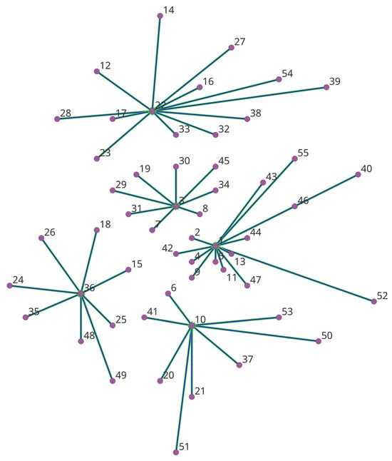
Figure 1.
The p-median problem and an optimal solution of Swain 55 node dataset using p = 5.
The p-median problem was first formulated using Integer Linear Programming by [8]. With a slight change in notation, the p-median problem can be formulated as follows:
: the sets of customer locations and candidate locations for facilities
: the population of each customer site .
: the distance from to .
The decision to make in the p-median problem is represented by two decision variables, and :
Now, the goal of the p-median problem is as follows:
Subject to:
The objective function (3) is used to minimize the service distance weighted by the amount of demand at each customer’s location. Constraints (4) are the assignment constraints stating that each customer should be assigned to one facility and one facility only. Constraint (5) maintains that exactly candidate sites should be selected as facilities. Constraints (6) maintain that a customer can only be assigned to a candidate site if there is an open facility there. Constraints (7) define the assignment variables as continuous variables between 0 and 1. Constraints (8) define the location variables as binary variables (0–1 variables).
The abovementioned definition of the p-median problem hides subtle details. The assignment variable is defined as a continuous variable that admits fractional values such as 0.2. Intuitively, however, there is no reason to make such fractional assignments because it is always the best to assign all customers at each demand location to its closest facility, since the assignment/allocation decision is made independently for each customer site. The definition of as fractional values is for computational reasons. Integer variables are costly in Integer Linear Programs. By comparison, continuous variables are much cheaper computationally. This is because efficient, polynomial time algorithms exist for Linear Programs (LPs, i.e., ILPs that do not have integer variables). By comparison, proper integer linear programs require a solution process, such as the branch and bound, that implicitly enumerates combinations of the integer variables. Additionally, there could be exponentially many combinations to enumerate, making ILPs much harder to solve than LPs.
Relaxing the integer requirement of the variables is legitimate only because of the integral assignment property [8]. In other words, there is always an integral solution at optimality. Even though one defines the assignment variable as fractional, one can always find an optimal integer solution. This relaxation reduces the number of integer variables by an order of magnitude. The informal notion of the integral assignment discussed so far is the first property that we will prove using proof language. We will show that, to fully express this property, it is necessary to rigorously define all the problem data as well as the notion of feasibility and optimality in a computer language.
2.2. Obnoxious/Adversary Facility Location and Closest Assignment Constraints
In the classic p-median problem, the objective function is distance minimizing. However, there are variants of the p-median problem in which the objective is distance maximizing. An example is the so-called interdiction models in adversary location modeling, represented by the r-interdiction median (RIM) model in [12]. From the perspective of an adversary, the RIM model aims to maximize the total service distance of the customers by removing facilities from the existing facilities. Equivalently, the goal of the RIM model can be viewed as to select facilities to keep so that the service distance is maximized. Even though the adversary’s goal is to disrupt service, each customer is still going to choose its closest facility to use. In ILP, the RIM model can be written as follows:
Subject to:
where is a set describing the order of closeness of facilities for a given customer . It is the set of facility sites that are closer to demand than facility is. The allocation variable has the same meaning as in the p-median problem. The location variable is 1 if an open facility is not interdicted by the adversary, and is 0 otherwise.
The classic p-median formulation cannot be used for RIM because the sense of the objective function is changed to maximization in (9) (or, equivalently, the p-median demand-constants become negative). To enforce the correct assignment of customers to their closest facilities, a type of explicit closest assignment constraints (ECA) [9,13] are required. In this formulation, the ECA constraint form in (12) is used [10]. Roughly speaking, it states that for a customer , when there are no closer facilities than , the assignment variable must be one.
In addition to interdiction models, there are also obnoxious facility and semi-obnoxious facility location problems, in which closest assignment constraints are required. For example, Church and Cohon [14] studied the location of nuclear power plants. They proposed that the perceived safety associated with a nuclear power plant was inversely proportional to the distance to the closest located plant. Therefore, they proposed maxian models that maximize the total distances from population centers to their closest nuclear power plant. Other examples of obnoxious and semi-obnoxious facilities include fire stations and sirens [15]. The reader is referred to [9,13] for more in-depth discussion of closest assignment constraints. In this article, we will show that the properties about constraint structures such as the ECA can also be formulated and proven in computerized proof languages. In Section 4, we will use the Lean language to prove that the ECA in (12) are correct.
2.3. Programs as Proofs
In this article, we use a proof language (Lean) based on the Curry–Howard isomorphism, in which the proof of a proposition is basically equated with a Haskell-style functional program. In principle, mathematics can be built based on functional programs. For example, natural numbers can be defined as an inductive data type in functional programming:
inductive Nat where
| zero : Nat
| succ (n : Nat) : Nat
which states that a natural number is either zero, or a successor (succ) of another natural number (n : Nat). The colon : in Lean is generally used as a typing annotation, e.g., to indicate that the type n is Nat. The vertical bar | is used to indicate alternatives in a definition. The definition Nat is recursive as some natural numbers are defined based on other natural numbers.
Mathematical operations or functions can also be defined recursively. For example, the add operation between two numbers a and b can be defined as follows:
def add : (a : Nat) → (b: Nat) → Nat
| a, Nat.zero => a
| a, Nat.succ b’ => Nat.succ (Nat.add a b’)
where the sum is just a if b is zero, and is defined recursively as the successor of a + b’ if b is the successor of some number b’. In the function add ((a : Nat) → (b: Nat) → Nat), the arrow → indicates a function type that takes some parameters (a and b of type Nat), and returns a final type (Nat). Again, the bar | indicates alternatives, and the double arrow => additionally indicates a mapping from certain input values or patterns to some return value.
In principle, one can continue to define subtraction between naturals, the integer numbers and their operations, the rationals and the reals, etc., in order to define all mathematical objects. This requires a tremendous amount of work. Fortunately, such definitions are provided in a standard Lean 4 library called mathlib, which we use extensively in this article. The reader is referred to the original Lean documentation (see, e.g., [16]) for details about the Lean language features and mathlib.
For the purpose of this article, we use the rational numbers (denoted as Rat or ℚ) to represent all numbers. This is sufficient because we deal with integer linear programs, and the rationals are closed under linear operations: addition, subtraction, multiplication and division (for non-zero divisors). We do not use real numbers for a subtle reason: operations for real numbers may be undecidable. For example, we cannot decide in finite time whether two real numbers 0.9999... and 1.000... are equal or not until we see the last digit. Therefore, we have to rely on external axioms about real numbers that the theorem prover cannot directly verify.
2.4. Dependent Types as Propositions
To prove theorems about the p-median problem, one needs to express them as propositions. Lean belongs to a class of proof languages based on dependent types and the program-as-proof paradigm (or the Curry–Howard isomorphism). In such languages, a theorem or proposition is equated to the type of data values, and each data value in that type is considered proof (or evidence) of the proposition. The type of all propositions is Prop. A theorem is false if there is no data value in its corresponding type, and is true if there exists a value (also known as evidence or proof) in its type. For example, Proposition 5 = 5 has a proof called rfl (which represents the reflexivity of values). By comparison, Proposition 5 = 5 ∧ 0 > 1 has no proof, because one cannot construct any proof of the second part of the proposition (0 > 1).
Under this paradigm, the logical implication → has a nice interpretation: given two propositions a and b, the proposition that a implies b is represented as a function f from a to b (of function type a→b). Supposing that such a function f exists, given the evidence ha of a, the result of applying f to ha (written in juxtaposition as f ha in functional languages) is precisely the evidence for b according to the typing rules for functions. Therefore, to prove the implication a → b, one just needs to construct a function of the right type (i.e., from a to b, which happens to be written as a → b in Lean). Once constructed, the function f serves as evidence of the type a → b (written as f : a → b).
As an example, to prove that a property a implies itself (i.e., a → a), we can construct a value of the corresponding type (namely, the identify function fun (x:a) => x):
def f1 (a: Prop) : a → a := fun (x:a) => x
In fact, a theorem in Lean is basically a Prop-valued definition. So, we can write the above equivalently as follows:
theorem f1 (a: Prop) : a → a := fun (x:a) => x
As another example, one can prove the conjunction 5 = 5 ∧ 1 = 1 by providing evidence for each part of the conjunction:
theorem t1 : 5 = 5 ∧ 1 = 1 := ⟨rfl, rfl⟩
2.5. Applications in Integer Linear Programming (ILP)
The program-as-proof idea is generally true in the proof language. A proposition p is true if it has a valid value hp that type-checks in the type, in which case we write hp : p. The functional program such as the identity function fun (x:a) => x and the pair ⟨rfl, rfl⟩ are often referred to as proof terms or simply proofs of the specific proposition. For the purpose of this article, we need to describe whether a variable in an ILP is valued as 0–1 to describe the integral assignment property. That is, the variable is either 0 or 1:
def binary (x : ℚ) : Prop := x = 0 ∨ x = 1
For this, we define a new type representing a property for rational number x (the type of this new type is Prop). Note that the new type x = 0 ∨ x = 1 is more complex than simple types such as int or string in conventional languages. This is because the type depends on the data value defined earlier in the context (x). So, the type can vary for different values of x. 0 = 0 ∨ 0 = 1 evaluates as true, and 2 = 0 ∨ 2 = 1 evaluates as false. This is why the type x = 0 ∨ x = 1 is called a dependent type.
Under the hood, the type a ∨ b is just a shorthand for another inductive data type Or. Just as with the Nat type, it has two ways of admitting values, one case for the left operand of ∨ and the other for the right operand:
inductive Or (a b : Prop) : Prop where
| inl (h : a) : Or a b
| inr (h : b) : Or a b
To construct evidence proof (or evidence) of a ∨ b, one just needs to construct a proof ha of a (in which case “inl ha” is a proof of a ∨ b) or, similarly, a proof hb of b. If a proof of a disjunction is already available, it can be used by case analysis, as shown in the lemma on binary values below:
theorem binary_le_one (x : ℚ) (hb: binary x) : x ≤ 1 := by
rcases hb with (h1 | h2)
. rw [h1]; norm_num
. rw [h2]
2.6. Constructing Proof Terms Using Tactics
This simple theorem (or lemma) demonstrates the general structures of many proofs. The theorem takes a rational number x and evidence hb of the fact that x is binary, and concludes that x must be less than or equal to one. Since the definition of binary x contains a disjunction (x = 0 ∨ x = 1), we can use case analysis on it. In the proof above, we first enter the “tactic” mode by using a by command. The tactics are basically program-writing programs for constructing proof terms. They serve the same role as the “macros” in many programming languages. Then, the rcases ... with ... tactic splits the disjunction goal (x = 0 ∨ x = 1) into two possibilities: one for the left branch h1 : x = 0, and one for the right branch h2 : x = 1.
In each case of the disjunction, we can use the hypotheses h1 or h2 to rewrite and simplify the goal. This is what the rw [h1] tactic does. In the first case, h1 : x = 0, the goal becomes 0 ≤ 1. Additionally, the tactic norm_num verifies such simple facts about numbers. In the second case, when h2 : x = 0, the goal becomes 1 ≤ 1, which can be verified automatically by rw itself. From the big picture, the rcases tactic decomposes the hypothesis hb into two smaller hypotheses h1 and h2.
2.7. Application of a Theorem
While one can theoretically prove the desired theorems regarding the p-median problem by applying the first principles presented so far, such proofs will be unnecessarily long. Instead of starting from scratch, we rely heavily on common theorems provided in the standard library. For example, there is a theorem regarding the transitivity of the ≤ relation:
lemma le_trans : a ≤ b → b ≤ c → a ≤ c
To apply a theorem, we just need to recall that a theorem is essentially a Prop-valued function, and we can use them as such. If we have a proof hab : 3 ≤ 4 and a proof hbc : 4 ≤ 5, to show that 3 ≤ 5, we only need to apply le_trans to them, so that le_trans hab hbc is evidence/proof of the goal (i.e., le_trans hab hbc : 3 ≤ 5).
As an alternative to writing the proof term directly, one can also use the apply tactic and write the following:
by
apply le_trans hab hbc
to build the proof term. Additionally, an input parameter can be left open using the placeholder _. The value of the placeholder will either be inferred from the context, or left as a new goal or value that remains to be constructed.
While there are many useful tactics in Lean, we primarily use four kinds of basic tactics in this article: apply, rewrite, case analysis, and by_contra. Roughly speaking, the apply tactic matches a theorem against the current goal and either closes the goal if it is a complete match or leaves unproven assumptions of the theorem as new goals. The rewrite (and rw) tactic substitutes equalities such as x = 5 into a goal or hypothesis. Case analysis allows us to split the current goal into two sub-goals depending on a condition (by_cases) or into multiple goals depending on the cases of an inductive data type (rcases). The by_contra tactic works by assuming that the current goal is False, and then identifying a contradiction in the hypotheses (such as h1 : x = 5 and h2 : x ≠ 5. On top of these, there are two types of higher-level tactics, namely simp and calc. The simp tactic (and its variants) semi-automatically rewrites and applies certain theorems to simplify the goal. The calc tactic is used for chaining the proofs of several equalities or inequalities into one (in)equality.
So far, this section has presented the properties of the p-median problem to be proven and the basic principles of theorem proving using a dependent type-language such as Lean. We have illustrated how the proof terms for a theorem can be constructed and applied in the program-as-proof paradigm. In the next section, we apply these principles to prove the fundamental properties of the classic p-median problem.
3. Proving the Integral Assignment Property
This section presents the basic definitions and formulations of the integral assignment property of p-median like problems in Lean (version 4). For exposition, we present the proofs about the main theorem and explain the required proof tactics along the way. The reader is referred to the Lean documentation [16] for additional details about the standard proof tactics and the mathlib library.
3.1. Basic Definitions
As a first step, one must choose an appropriate representation for the data of the p-median problem. In particular, one needs to define constants such as the sets , the distance matrix as well as the decision variables , , as described in the background section. There is a decision to make here. One possibility is to use the data structure in common programming languages, such as lists (or arrays), to represent these mathematical objects. In this representation, the customer sites could be each represented as a list, and the distance matrix could be represented as a list of lists, etc. However, the use of a list is problematic for several reasons. First, it is necessary to ensure that the lengths of the lists in various definitions match. For example, the sizes of the lists for the distance matrix must match the sizes of . There is no guarantee that the input data will be consistent in size. One could possibly impose the requirement of the sizes as additional propositions, but this would be cumbersome. Second, there is no guarantee that each list will be a mathematical set. Lists and arrays in regular programming languages allow duplicate values while mathematical sets do not. Third, and more importantly, one cannot make the necessary assumptions about lists (e.g., the uniqueness of elements) and one has to prove many theorems about the problem data from scratch.
For these reasons, we choose to represent the data, which are essentially mathematical arrays on index sets (one or two indices), as functions from two finite sets and to the numbers. For example, we can define the assignment variable as a function from the finite sets (called Finset in Lean) I and J to the rational numbers ℚ:
def x [LinearOrder α] (I: Finset α) (J: Finset α) : α → α → ℚ := sorry
In this prototype definition, x is the name of the array and α is the type of the indices. These could be ID numbers or names of the customer or facility sites. The only requirement for α is that it be a linear order (which allows one to compare and sort the indices). I, J are each defined as a finite set (Finset) of base type α. The two-dimensional array x is defined as a function from α and α to ℚ, with an understanding that the x i j value is non-zero only when the index i : α is in I (written as i ∈ I in Lean) and when j ∈ J. In other words, the support of the function x is I × J. sorry is a placeholder representing a missing value. We present this prototype definition only to illustrate the finite set based arrays. In the actual proof, we do not pre-define any of these arrays. Instead, we use them as input parameters to theorems and definitions, meaning that, given a mathematical array x on the index I, J, a certain property holds. For the rest of this article, we refer to such mathematical arrays simply as arrays.
With this convention, we can translate the basic definitions of the p-median problem to Lean in a notation that is almost identical to the ordinary mathematical notation in (3) through (8). For example, the definition of the assignment variable in (7) can be written as follows:
def xDef [LinearOrder α] (I: Finset α) (J: Finset α) : (∀ i ∈ I, ∀ j ∈ J, 0 ≤ x i j ∧ x i j ≤ 1) := sorry
Note that, in the example given above, the array value of x at (i, j) is written as x i j, which stands for the application of the function x to the parameter values i and j. This is the common syntax for function application in functional languages such as Haskell and Lean. One advantage of such syntax is that it makes it easy to convert multi-argument functions into unary functions in a process called currying. Roughly speaking, this means that given the binary function x, one can only partially apply it to one argument i. For each i, the result (x i) is a unary function that takes an argument j, and returns the final number. By currying, partially applied functions become meaningful objects. Here, the two-dimensional array, when partially applied to one index value, becomes a one-dimensional array. Currying is a useful feature and will be extensively used in the rest of this article. Other than currying, the language used in the definition is quite conventional. We used universal quantifiers ∀ i ∈ I, ∀ j ∈ J, ... to express that for each i in I, j in J, x i j must meet certain conditions.
The definition above is again a prototype containing a sorry value. In the real definition, we use both x and its defining property xDef as arguments for theorems. The full definition for the problem data and requirements of the p-median problem is defined in a definition called pmed_feasible as follows:
def pmed_feasible [LinearOrder α] (I: Finset α) (J: Finset α) (p : ℕ) (hp1 : 0 < p) (hp2 : p ≤ J.card)
(a: α → ℚ) (d: α→α→ ℚ)
(y : α → ℚ) (x: α→α→ ℚ)
: Prop :=
(∀ i ∈ I, ∀ j ∈ J, 0 ≤ x i j ∧ x i j ≤ 1) ∧ -- xDef
(∀ j ∈ J, binary (y j)) ∧ -- yDef
(∀ i ∈ I, (∑ j ∈ J, x i j) = 1) ∧ -- cAssignment
(∑ j ∈ J, y j = p) ∧ -- cCardinality
(∀ i ∈ I, ∀ j ∈ J, x i j ≤ y j) -- cBalinski
This is a complete description of the model constraints in (4) through (8). Note that the contents after -- are comments for the human reader and are ignored by Lean. In this definition, we define the two finite index sets I and J, the number of facilities to locate (p), the distance matrix (d), the decision variables (x and y), and the list of properties that x and y must satisfy for them to be a valid solution to the p-median problem. In addition, we also define the requirements on the problem data as Prop valued input arguments. In particular, we require that the natural number p be positive with hp1 as evidence, and that p is less than or equal to the size of the candidate set J with hp2 as evidence. The definition of pmed_feasible serves both as a goal to prove (that something is feasible) and as a contract (that if something is known to be a feasible solution, these properties are guaranteed to be true).
Note that in above, we used ordinary mathematical symbols such as “∑” for summation in, e.g., “∑ j ∈ J, y j” in the Lean definition. This is possible because of Lean 4′s macro system that allows one to expand a syntax such as “∑ x ∈ s, f x” in to a regular Lean term, which in this case is Finset.sum s f and stands for the sum of f x when x ranges over a finite set s. Likewise, other syntax/notation in ordinary mathematics such as the universal quantifier “∀”, the existential quantifier “∃”, the set notation “{x ∈ S | …}”, etc., can be encoded and translated to the core language, making it convenient to write mathematics in Lean.
The objective function (3) of the p-median problem can be defined using the following two functions:
def dot [LinearOrder α] (J: Finset α) (x_i : α → ℚ) (y_i : α→ ℚ) : ℚ :=
∑ j ∈ J, x_i j * y_i j
def obj_pmedian [LinearOrder α] (I: Finset α) (J: Finset α) (a: α → ℚ) (d: α→α→ ℚ) (x: α → α → ℚ) (y: α → ℚ) : ℚ :=
∑ i ∈ I, a i * dot J (x i) (d i)
The dot function defines the inner product between two finitely supported arrays on the same index set J. The notation used in the function body is the same as that in ordinary mathematics. We use ∑ j ∈ J, f j to express the sum (over J) of some value f j that depends on j ∈ J. To express the summation over a subset of J where certain condition p j holds, we can write as ∑ j ∈ {x ∈ J | p x}, x_i j * y_i j, where {x ∈ J | p x} represents the subset in which the condition p holds. The obj_pmedian function then defines the objective function (3) as the sum of the inner products of the i-th row of the assignment variable (as a matrix) and the i-th row of the distance matrix d. Note that we used currying to represent the i-th row of a two-dimensional array.
3.2. Formulation of the Properties
With the basic definitions in place, we can now formulate the optimality conditions and the closest assignment conditions. A solution to an optimization problem is optimal if it is feasible and its objective function value is less than or equal to the objective value of any other feasible solutions (for a minimization problem). This is characterized in logic by the following definition.
def pmed_optimal [LinearOrder α] (I: Finset α) (J: Finset α) (p : ℕ) (hp1 : 0 < p) (hp2 : p ≤ J.card)
(a: α → ℚ) (d: α→α→ ℚ)
(y : α → ℚ) (x: α→α→ ℚ)
: Prop :=
pmed_feasible I J p hp1 hp2 a d y x ∧
∀ x’ y’, pmed_feasible I J p hp1 hp2 a d y’ x’ → obj_pmedian I J a d x y ≤ obj_pmedian I J a d x’ y’
The integral assignment property states that among the optimal solutions, there always exists an integral one. Our idea of proving this is that, given any optimal solution that is possibly fractional, we can always construct a new solution that is integral. If the new solution is better than an optimal solution, then it must be optimal itself. To encode this logic, we prove an auxiliary theorem pmed_optimal_of_le_optimal as follows:
theorem pmed_optimal_of_le_optimal [LinearOrder α] (I: Finset α) (J: Finset α) (p : ℕ) (hp1 : 0 < p) (hp2 : p ≤ J.card)
(a: α → ℚ) (d: α→α→ ℚ)
(y : α → ℚ) (x: α→α→ ℚ)
(hopt : pmed_optimal I J p hp1 hp2 a d y x)
: ∀ x’ y’, pmed_feasible I J p hp1 hp2 a d y’ x’ → obj_pmedian I J a d x’ y’ ≤ obj_pmedian I J a d x y
→ pmed_optimal I J p hp1 hp2 a d y’ x’
:= by
intro x’ y’ hfeas’ h_le_opt
dsimp [pmed_optimal]
constructor
· exact hfeas’
· intro x’’ y’’ hfeas’’
calc obj_pmedian I J a d x’ y’
_ ≤ obj_pmedian I J a d x y := h_le_opt
_ ≤ obj_pmedian I J a d x’’ y’’ := hopt.2 x’’ y’’ hfeas’’
The name of the theorem (pmed_optimal_of_le_optimal) follows Lean’s convention that states the conclusion of the theorem first (pmed_optimal, that a solution is optimal), which is followed by (of) and then by the main hypotheses (le_optimal, that the solution is less than or equal to an optimal solution in terms of objective values). In this theorem, the data definitions (a, d, x, y) are given as input arguments of the theorem as usual. After that, (hopt : pmed_optimal I J p hp1 hp2 a d y x) is an assumption that an optimal solution x, y exists. Then, the goal after the top-level : states that for any feasible solution x’, y’, if its objective value is less than or equal to the optimal objective, then x’, y’ must be optimal as well.
The lines after := by are the tactics used to construct a proof. The first line intro x’ y’ hfeas’ h_le_opt introduces the variables in and hypotheses for the goal into the proof context and assigns the names x’, y’, hfeas’, h_le_opt to them, so that hfeas’ : pmed_feasible I J p hp1 hp2 a d y’ x’, etc. The second line dsimp [pmed_optimal] expands the definition of pmed_optimal into its body in the goal. By definition, pmed_optimal .. y’ x’ has two components: pmed_feasible .. y’ x’ and obj_pmedian .. y’ x’ ≤ obj_pmedian .. y’‘ x’‘ for any other feasible solution x’‘, y’‘. This can be decomposed into two sub-goals using the constructor tactic in the third line. The first sub-goal about the feasibility of x’ y’ is already in the current list of assumptions in this context (as hfeas’). So, we directly apply it with the exact hefeas’ tactic. Note that the exact tactic is just a terminal version of the apply tactic that requires its argument term to fully match the current goal.
For the second sub-goal obj_pmedian .. y’ x’ ≤ obj_pmedian .. y’’ x’’, we use a calc block, which decomposes the equality or inequality into a nice chain of intermediate proof steps, each with its own justification/evidence. Here, the first step is as follows:
obj_pmedian I J a d x’ y’
_ ≤ obj_pmedian I J a d x y := h_le_opt
which states that the given feasible solution x’, y’ is better than an optimal solution x, y. This is one of the assumptions (h_le_opt) used here directly as the evidence for this step.
The second step is as follows:
_ ≤ obj_pmedian I J a d x y := ..
_ ≤ obj_pmedian I J a d x’’ y’’ := hopt.2 x’’ y’’ hfeas’’
states that the optimal solution x, y should be better than any other feasible solution x’’, y’’. The evidence of this step is exactly the second component of optimality for x, y, which expressed in proof terms is hopt.2 x’’ y’’ hfeas’’. The calc block is readable as it explicitly shows each intermediate goal and the justification to reach it.
3.3. Constructing an Integral Optimal Solution
The remaining task for proving the integral assignment property is to construct an integral solution that is better than a given optimal solution. Informally, this can be accomplished as follows. Given an optimal solution x, y, one can keep the location decision y, and reconstruct a set of new assignment variables x’ in which all demand at i ∈ I is assigned to a single y j, namely, the closest y j to i. This new solution x’ is clearly integral. One only needs to prove that it is feasible and optimal.
In the computerized proof, we have to be complete and leave no details out or assume that they are “clearly” true. The computer does not know that. To construct the new assignment variable x’, we define a new function called one_hot to represent this one-hot encoding of assignments (i.e., among all candidate sites, only one is non-zero).
def one_hot [LinearOrder α] {J: Finset α} (j0 : α) (j0mem: j0 ∈ J): (α→ ℚ) :=
fun j => if j = j0 then 1 else 0
Given a position j0, the one_hot function simply maps its argument to one at position j0, and to zero in all other positions. We also prove two simple properties about the one-hot encoding:
First, a one-hot encoded array is binary (i.e., all its entries are binary). This is proven by a simple case analysis on whether the index j is equal to the non-zero position. In either case, the one_hot value, after proper expansion of the definitions, is 1 or 0, which is binary. Note that we use ; to sequence two tactics in one line, and use <;> to tell Lean to apply the second tactic to every possible branch/case generated by the first tactic.
theorem one_hot_binary [LinearOrder α] {J: Finset α} (j0 : α) (j0mem: j0 ∈ J): ∀ j ∈ J, binary (one_hot j0 j0mem j) := by
intro j jmem
dsimp [one_hot, binary]
by_cases h : j = j0 <;> simp [h]
Second, a one-hot encoded array adds up to one. This involves using the mathlib theorem Finset.sum_ite_eq’ (where the “ite” stands for if-then-else) to split the sum into two sums depending on whether j = j0 or not. We can do so because the one-hot encoding is essentially a conditional value. Then, after simplification, the first sum is 1 and the second is 0.
theorem one_hot_sum_one [LinearOrder α] {J: Finset α} (j0 : α) (j0mem: j0 ∈ J): ∑ j ∈ J, (one_hot j0 j0mem) j = 1 := by
dsimp [one_hot]
rw [Finset.sum_ite_eq’] ; simp
exact j0mem
The newly constructed one-hot encoding array x’ i must have non-zero entries only at the open facility positions. Elsewhere, we must have x’ i j = 0. To express this condition, we define the support of an array as follows:
def supp [LinearOrder α] (J: Finset α) (J’: Finset α) (y : α → ℚ) : Prop := ∀ j ∈ J, j ∉ J’ → y j = 0
Then, for a feasible solution x, y, we can show that the support of the newly constructed x’ i is indeed the set of open facilities {j ∈ J | y j = 1}, as stated in the following theorem (see the proof in the Appendix A):
theorem supp_x_of_pmed_feasible [LinearOrder α] (I: Finset α) (J: Finset α) (p : ℕ) (hp1 : 0 < p) (hp2 : p ≤ J.card)
(a: α → ℚ) (d: α→α→ ℚ)
: pmed_feasible I J p hp1 hp2 a d y x → ∀ i ∈ I, supp J { j ∈ J | y j = 1} (x i)
The properties of the main construction x’ is described by the following theorem:
theorem assign_closest_i [LinearOrder α] {J: Finset α} {J’: Finset α} (hJne: J’.Nonempty) (hsub: J’ ⊆ J) (d_i : α→ ℚ): ∃ x_i0, (∀ j ∈ J, binary (x_i0 j)) ∧
supp J J’ x_i0 ∧ (∑ j ∈ J’, x_i0 j = 1) ∧
∀ (x_i: α → ℚ), (∀ j ∈ J, 0 ≤ x_i j) → (∑ j ∈ J, x_i j = 1) → supp J J’ x_i →
dot J x_i0 d_i ≤ dot J x_i d_i
It states that given an assignment x_i of a fixed customer i to a nonempty subset of facilities J’ ⊆ J, there always exists a binary assignment x_i0 that is constrained to the same subset J’, and has a smaller distance sum. The theorem is not difficult to prove given the one-hot construction we described above. However, its proof is too long to present here, and we only report the main idea. Basically, for each x_i, we construct an array containing pairs of (d_i j, j), where j is an index in J and d_i j = d i j is the distance from i to j. We then define a min function on these distance–index pairs according to the lexicographic order, and then pick the smallest pair in the array. This pair has the minimum distance along with the corresponding index j0. Now, we can choose x_i0 = one_hot j0 .., and prove that its weighted total distance dot x_i’ d_i is less than or equal to the original dot x_i d_i because x_i’ has all the weights on the smallest distance index, whereas x_i may have fractional assignments distributed to other sites. Note that the conclusion of the theorem (about x_i0) is relatively long. It is because this theorem is the site where the one-hot encoded array x_i0 is constructed. This is the most convenient site to prove various properties about the construction (e.g., the one-hot encoding being binary), and we then need to export these properties to users of this theorem.
The theorem assign_closest_i describes properties of each row of the assignment matrix x’ i (representing the one-hot assignment). To describe the properties of the entire matrix x’, we have another auxiliary theorem in which we prove that the rows x’ i, when put together into a solution x’, y, constitute a feasible solution of the feasible solution. The proof is long and routine, and mainly proves that the feasibility conditions are met. For example, the cardinality constraints are met because the new solution x’,y shares the same location variable y with the existing solution. The condition in xDef holds by the nature of the one-hot encoding, etc. We again present below its statement only for brevity. The theorem states that given an optimal solution x y, there exists a new solution x’ (the one-hot encoded assignment) that is feasible and has smaller distance sums than any other feasible solutions.
theorem assign_closest_feasible [LinearOrder α] (I: Finset α) (J: Finset α)
(p : ℕ) (hp1 : 0 < p) (hp2 : p ≤ J.card) (a: α→ ℚ) (d: α → α → ℚ)
: ∀ x y, pmed_optimal I J p hp1 hp2 a d y x →
∃ x0, (pmed_feasible I J p hp1 hp2 a d y x0) ∧ (∀ i ∈ I, ∀ j ∈ J, binary (x0 i j)) ∧
∀ (x’’: α → α → ℚ), pmed_feasible I J p hp1 hp2 a d y x’’ →
∀ i ∈ I, dot J (x0 i) (d i) ≤ dot J (x’’ i) (d i)
3.4. Main Theorem for Integral Assignment
With the auxiliary theorems and constructions above, we can prove the main theorem about the integral assignment property. The statement of the theorem is the same as the informal description of the integral assignment property: that among optimal solutions, an integral one exists.
theorem integral_assignment [LinearOrder α] (I: Finset α) (J: Finset α)
(p : ℕ) (hp1 : 0 < p) (hp2 : p ≤ J.card) (a: α → ℚ) (ha : ∀ i ∈ I, 0 ≤ a i) (d: α→α→ ℚ)
: ∀ x y, pmed_optimal I J p hp1 hp2 a d y x → ∃ x’ y’, pmed_optimal I J p hp1 hp2 a d y’ x’ ∧ ∀ i ∈ I, ∀ j ∈ J, binary (x’ i j)
The overall workflow of the proof is presented in Figure 2. The proof is constructive in that given an optimal solution x, y with possibly fractional assignment variables (in the left of Figure 2), we construct an integral solution x0, y that is better than the optimal. Then, x0, y must be the desired integral optimal solution we seek (by pmed_optimal_of_le_optimal near the bottom). The construction of x0, y itself is based on reusing the set of facilities in y and reconstructing the assignment variable x0 using the one_hot function (at the top), which by nature generates integral assignments. In theorem assign_closest_i, we assign each customer i to the closest facility in y. We then prove that x0, y is feasible in assign_closest_feasible, and therefore optimal in integral_assignment. During the proof, evidence of the feasibility (of the type pmed_feasible) of the old solution and the improved solution is passed around to eventually establish the optimality of the improved solution x0, y.
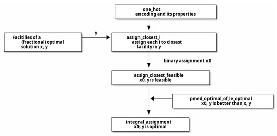
Figure 2.
The main workflow of the computerized proof of the integral assignment property for the p-median problem.
4. Proving the Closest Assignment Constraints
As mentioned in the background section, in certain applications such as obnoxious facility location and adversary location, variants of the p-median problem can have negative demand. Consequently, these models would naturally assign customers to the farthest facilities. However, each customer is still impacted or served by the closest facility. This means that explicit closest assignment (ECA) constraints such as (12) are required to force the assignment variable to be targeted towards the closest open facility.
Using the same problem definitions as in the previous section, we can also prove the correctness of the ECA constraint in (12) due to [10]. We first translate the set C in the ECA into the following definition:
def C [LinearOrder α] (I: Finset α) (J: Finset α) (d: α → α → ℚ) (i : α) (j : α) : Finset α :=
{q ∈ J | d i q < d i j}
Other than the additional definition about the finite index sets I, J, the definition of C is exactly the same as in the ILP formulation. Additionally, C I J d i j (written as C i j for short hereafter) represents the set of facilities that are closer than j for a customer i. Then, the correctness of the ECA constraint can be stated and proven as follows:
theorem ca_rr_correct [LinearOrder α] (I: Finset α) (J: Finset α)
(a: α → ℚ) (d: α→α→ ℚ)
(y : α → ℚ) (x: α→α→ ℚ)
(xDef: ∀ i j, 0 ≤ x i j ∧ x i j ≤ 1)
(yDef : ∀ j, binary (y j))
(cAssignment: ∀ i, (∑ j ∈ J, x i j) = 1)
(cBalinski: ∀ i j, x i j ≤ y j)
(cCA: ∀ i j, ∑ q ∈ C I J d i j, y q + x i j ≥ y j)
: ∀ i j, y j = 1 → (∀ k, y k = 1 → d i j ≤ d i k) → x i j = 1 -- CA condition
:= by
intro i j
intro yjIsOne
intro dijLtDik
have h0 : ∀ q ∈ C I J d i j, y q = 0 := by
intro q hq
simp [C] at hq
have h11 := not_imp_not.2 (dijLtDik q)
rw [lt_iff_not_ge] at hq
exact binary_zero_of_not_one (y q) (yDef q) (h11 hq.2)
have h1 : ∑ q ∈ C I J d i j, y q = 0 := Finset.sum_eq_zero h0
have h2 := cCA i j
rw [h1, yjIsOne] at h2
simp at h2
have ⟨_, h3⟩ := xDef i j
apply le_antisymm h3 h2
The theorem ca_rr_correct has similar data definitions a, d, x, y in the statement, as well as similar assumptions about the feasibility of the solution x y. Note that there is no assumption that demand a is positive here. A new input argument is proof (cCA) that the ECA constraint is satisfied by x, y. The conclusion is a logical expression of what would happen if the ECA constraint was correct. That is, for each open facility (for which y j = 1), if no facility is closer than j for customer i, then the assignment variable x i j should be forced to 1.
Compared with the previous section, the proof here is relatively short. After introducing the universally quantified variables and the assumptions of the goal, we prove several intermediate goals, namely h0, h1, h2, and h3. h0 states that for each candidate site q in C i j, y q must be zero. This is proven by simplifying the definition of C with the hypothesis that q ∈ C i j. This leads to the condition hq : q ∈ J ∧ d i q < d i j. The assumption dijLtDik : ∀ k, y k = 1 → d i j ≤ d i k, when applied to q (i.e., when k is replaced by q), implies that y q = 1 → d i j ≤ d q. not_imp_not is an logical equivalence ¬a → ¬b ↔ b → a. not_imp_not.2 stands for the second direction (←) of the equivalence. Therefore, not_imp_not.2 (dijLtDik q) has type: ¬d i j ≤ d i q → ¬y q = 1, where ¬ a stands for the negation of a proposition a. The rest of the proofs in h0 basically says that since d i q < d i j, we know ¬y q = 1. Then, according to the definition of y (yDef), y q is binary. From binary_zero_of_not_one, we know that q = 0.
Since every y q in C i j is zero by h0, we know that the sum of these y qs is zero, by applying a mathlib theorem Finset.sum_eq_zero on h0. Then, we can rewrite the sum to zero in the ECA constraint for the current i and j. We can also rewrite y j to 1 by the assumption that yjIsOne. The CA constraint simplifies to the following:
h2 : 1 ≤ x i j.
However, from the definition of x (xDef), we already know that 1 ≥ x i j. Then, we know that 1 = x i j, by the anti-symmetry of the ≤ relation (le_antisymm). The proof above is quite low-level in logic. One needs to be thoughtful and plan ahead as to which intermediate goals are needed to reach the main goal successfully. One may fail to reach the final goal due to errors or a wrong direction of the proof leading nowhere. However, if the goal is ever reached using a proof, one can be sure that the theorem cannot be mistaken.
5. Discussion
In this section, we discuss a few design choices we made in this article including the choice of proof languages, the model representation, as well as specific choices made in the Lean proofs.
5.1. Why ILP?
In this article, we introduced ILP as a mathematical language for theorem proving. We chose ILP as the language for a number of reasons. Firstly, the ILP model for an optimization problem is the specification and the program at the same time. It is a specification in that we use the set theoretical language in ILP to precisely describe the objects (e.g., I and J), relations (e.g., the closeness set C), the constraints, and the objective of the model, so that there is no ambiguity about the meaning of the problem. It is a program because despite the conciseness of ILP models, they are complete and executable by off-the-shelf solvers such as CPLEX. The solvers can tell in the end whether the problem has an optimal solution or is infeasible/unbounded. Secondly, the set of operations in ILP is constrained: only linear arithmetic with possible integral conditions is allowed. Consequently, one only needs to use and extend theorems about linear equalities/inequalities and integer (or 0–1 valued) numbers. Thirdly, ILP is widely used in describing spatial optimization models and can be easily understood by researchers in the field.
Conceivably one could use alternative descriptions of spatial optimization problems. One could use, e.g., set theory alone to describe the optimization problem and then try to prove its properties. However, there will be more unknowns and proof obligations, as the unconstrained set theory is much more powerful. For this description to be useful, one would need to prove that the optimal solution can be found in a finite amount of time. For example, one could use an algorithm in an imperative language to describe how the optimal solution can be found. Then, one has to prove additional properties such as the termination of the algorithm, and that the state of the program at termination is as intended, etc. Using ILP (if appropriate for the problem) makes it unnecessary to prove such properties as they come for free because of the ILP solvers (and theory).
5.2. Why Lean?
There are many proof languages, such as Coq, Isabelle, HOL4, Agda, and Idris2, among others. We actually tried some of these languages before settling on Lean 4. Our choice of Lean over the other languages is based on a number of unique features of Lean. Firstly, we targeted Lean and Idris2 because these two proof languages are relatively new and more importantly, can both be used as a proof language and as a general purpose programming language. By comparison, conventional proof languages are primarily for theorem proving. In our opinion, this fits naturally to the program-as-proof paradigm and unifies proving and programming. However, Idris2, despite its many attractive features, does not have tactics or a large library of theorems such as Lean’s mathlib.
Secondly, we chose Lean because of our preference on constructive proofs and the program-as-proof way. In our opinion, such proof languages require fewer axioms and external assumptions. Isabelle, for example, assumes that all types are nonempty, and any type is inhabited by an value called “undefined”. While Isabelle is certainly consistent, we preferred Lean 4 because it does not require such assumptions to work.
Thirdly, Lean 4 has a powerful macro system in the Lean language itself. We also made some attempts with Coq, but preferred Lean 4 because the tactical language of Lean is written in Lean itself. In Coq, this is accomplished by a separate language.
That being said, the other proof systems do have their advantages. Isabelle and Coq have powerful proof automation. Isabelle, for example, has the well-known sledgehammer command that can automatically find some intermediate proofs. The user should choose the proof system based on informed decision and the specific task at hand.
5.3. Design Choices in Lean Proofs
The first choice made in the proofs was about the data representation for arrays. We used a Finset α I to denote the support of an array, and used it in quantifiers and summations such as ∀ i ∈ I, p i and ∑ i ∈ I, y i. The property p : α → Prop or value y : α → ℚ is defined directly on the index type α. Alternatively, one could use the Finset I directly as the index type. Then, the array could be defined as y : I → ℚ (i.e., from I rather than α to ℚ). (Under the hood, what happens is that the Finset is converted to a “subtype”, which we will not discuss here). The advantage of this approach is that an array defined in this way carries its domain or support with it. One does not have to keep track of the fact that the assignment variable x : α → α → ℚ is defined on the finite sets I and J, or worry about using the wrong sets as input to x. Instead, the finite sets are directly in the type x : I → J → ℚ. This makes the proof more succinct and less error-prone. With this method, quantification and sums can be written as ∀ i : I, p i and ∑ i : I, y i (note the use if i : I instead of i ∈ I)
The reason we did not use Finset directly as the index type is rather pragmatic. We found that there are more familiar theorems about summations in the set form ∑ i ∈ I, y i than those about the type form ∑ i : I, y i (see, e.g., the theorem Finset.sum_eq_zero above). Yet another possibility is to create our own data type to represent the mathematical array. However, we would have the same problem of needing to build the system of useful theorems (i.e. an API) about the array and its operations. It boils down to the cost–benefit ratio.
We also made a choice between the implicit and explicit arguments in the definitions. Dependent-type languages such as Lean allow certain arguments to be inferred automatically (using the dependency between the arguments). For example, in the definition of pmed_feasible below, the value of p could have been inferred from the evidence hp1 of 0 < p. If we provide evidence proof of 0 < 5 as hp1, we know that p must be 5.
def pmed_feasible [LinearOrder α] (I: Finset α) (J: Finset α) (p : ℕ) (hp1 : 0 < p) (hp2 : p ≤ J.card)
(a: α → ℚ) (d: α→α→ ℚ)
(y : α → ℚ) (x: α→α→ ℚ)
Therefore, this declaration could have been defined as follows:
def pmed_feasible [LinearOrder α] (I: Finset α) (J: Finset α) {p : ℕ} (hp1 : 0 < p) (hp2 : p ≤ J.card)
(a: α → ℚ) (d: α→α→ ℚ)
(y : α → ℚ) (x: α→α→ ℚ)
where {p : ℕ} indicates that p is implicit and omitted when the definition is applied. Implicit arguments are extensively used in proofs. They make proofs more succinct by omitting the unnecessary parameter p (since its value can be inferred from hp1). We did not use implicit arguments much in this article primarily for clarity.
Another choice we made is to always have each definition carry all of its arguments. For example, pmed_feasbile above carries all the data and properties I, J, p, hp1, hp2, a, d, y, x. This is somewhat verbose. In Lean, it is possible to extract such declarations using the variable command and section. Again, we chose to let each definition carry all of its arguments primarily for clarity (so that each definition is self-contained).
6. Conclusions and Future Work
The p-median problem is a prototypical model in location analysis and GIS. It has been widely used in different disciplines ranging from transportation and logistics to facility layouts in the public and private sectors. Due to its generality, it has also been used as a unifying location model upon which other location models are based [6,7,17]. Therefore, it is important to study and understand the properties of the p-median problem and its variants. Two such important properties are integral assignment (an integral solution always exists at optimality) and closest assignment (with proper constraints, customers can be assigned to the closest facility).
Conventionally, such properties of location-allocation models have been proven informally. In this article, we present a computerized proof for each of these fundamental properties using the Lean theorem prover. A computerized proof starts with basic definitions and theorems and a proof, once constructed, is guaranteed to be correct. We have shown how the p-median problem can be characterized fully using the dependent-type system in Lean. We then show how one can prove two different types of theorems regarding the optimality conditions and the correctness of hard constraints. The computerized proofs are long compared to informal proofs. However, this article demonstrates that a structured and readable proof is at least feasible.
Potentially, the proof method presented in this paper can be used in other spatial optimization problems to improve their ILP models, by allowing the relaxation of integrality constraints or other constraints that are provably unnecessary. Theorems about model structures (such as the CA constraints) can also serve as a logical specification of a model’s intended behavior, and provide a guarantee that the specification is met by the model formulation.
There are several directions worthy of future investigation. First, the theorems in this article could be refactored into more generic ones suitable for other optimization models or Integer Linear Programming in general. We attempted to refactor a few basic lemmas regarding binary decision variables. However, more could be formulated regarding linear constraints and objective functions. Second, new representations could be defined for the mathematical array as well as its associated properties and theorems. Finally, it would be interesting to investigate other forms of representation of the p-median problem (other than ILP) and compare theorem proving in these forms with proofs in ILP. This is left for future research.
Author Contributions
Conceptualization, Ting L. Lei and Zhen Lei; Methodology, Ting L. Lei; Software, Ting L. Lei and Zhen Lei; Validation, Ting L. Lei; Formal analysis, Ting L. Lei; Investigation, Ting L. Lei and Zhen Lei; Resources, Ting L. Lei; Data curation, Ting L. Lei; Writing—original draft, Ting L. Lei and Zhen Lei; Writing—review & editing, Ting L. Lei and Zhen Lei; Visualization, Ting L. Lei and Zhen Lei; Supervision, Ting L. Lei; Project administration, Ting L. Lei and Zhen Lei; Funding acquisition, Zhen Lei. All authors have read and agreed to the published version of the manuscript.
Funding
This research was partly supported by Natural Science Foundation, Grant number BCS-2215155 and National Natural Science Foundation of China (NSFC), Grant number 41971334.
Data Availability Statement
The data that support the findings of this study are available upon reasonable request.
Conflicts of Interest
The authors declare no conflict of interest.
Appendix A
In this appendix, we list the proofs of some of the theorems in Section 3.
Appendix A.1. The Theorem Supp_x_of_Pmed_Feasible
theorem supp_x_of_pmed_feasible [LinearOrder α] (I: Finset α) (J: Finset α) (p : ℕ) (hp1 : 0 < p) (hp2 : p ≤ J.card)
(a: α→ ℚ) (d: α → α → ℚ)
: pmed_feasible I J p hp1 hp2 a d y x → ∀ i ∈ I, supp J { j ∈ J | y j = 1} (x i)
:= by
intro ⟨xDef, yDef, cAssign, cCard, cBalinski⟩
intro i imem -- ∀ i ∈ I
dsimp [supp]
intro j jmem jnmem -- ∀ j ∈ J, j ∉ J’
by_contra! contra
have h1 := calc 0
_ < x i j := lt_of_le_of_ne (xDef i imem j jmem).1 (ne_comm.1 contra)
_ ≤ y j := cBalinski i imem j jmem
have h2 : y j = 1 := binary_one_of_not_zero (y j) (yDef j jmem) (ne_of_gt h1)
have h3: j ∈ {j ∈ J | y j = 1} := Finset.mem_filter.2 ⟨jmem, h2⟩
contradiction
In the proof, we first introduce the pmed_feasible assumption, and immediately decompose it into the constraints of the p-median ⟨xDef, yDef, cAssign, cCard, cBalinski⟩. We then introduce the argument ∀ i ∈ I, which is really a shorthand for ∀ i : α, i ∈ I. So, we use two names i and imem to represent the value of i and the assumption imem that it is a member of I. We then expand the definition of support supp, and similarly introduces j and its membership and non-membership assumptions ∀ j ∈ J, j ∉ J’. At this point, the goal to prove is x i j = 0 (since j is supposed to be outside the support). We then prove the goal by contradiction and assuming the goal is not true x i j ≠ 0 (as a new assumption named contra). In the next three steps, we first prove in h1 that y j > 0 using the definition of x (0 ≤ x i j), the assumption x i j ≠ 0, and then the Balinski constraint (cBalinski). Since y j is non-zero and binary, we know that it is one by binary_one_of_not_zero. Then, we know that j ∈ J’, where J’ = {j ∈ J | y j = 1}. This is a contradiction with the assumption jnmem: j ∉ J’. So, we must have x i j = 0. The auxiliary theorems lt_of_le_of_ne, ne_comm, ne_of_gt and Finset.mem_filter are from the standard Lean library and state simple facts about inequalities and Finsets. We do not discuss them here for space reasons.
Appendix A.2. The Main Theorem
Below is the proof of the main theorem integral_assignment. The main idea is to apply the theorem assign_closest_feasible to obtain the one-hot encoded assignment variable x’, as well as the properties it has been proven to have so far. The result is an existentially quantified statement that ∃ x0, (pmed_feasible I J p hp1 hp2 a d y x0) ∧ ... We use Classical.choose and Classical.choose_spec to obtain the value and the properties of the new assignment variable x’, including its feasibility (hfeas’) and integral property (hbin_x’). We prove the optimality of x’, y by showing with a calc block that its objective function value is better than the known optimal solution x, y, assuming the demand is positive (ha). Then, by the theorem pmed_optimal_of_le_optimal, we conclude that the new solution is indeed optimal and integral.
theorem integral_assignment [LinearOrder α] (I: Finset α) (J: Finset α)
(p : ℕ) (hp1 : 0 < p) (hp2 : p ≤ J.card) (a: α→ ℚ) (ha : ∀ i ∈ I, 0 ≤ a i) (d: α → α → ℚ)
: ∀ x y, pmed_optimal I J p hp1 hp2 a d y x → ∃ x’ y’, pmed_optimal I J p hp1 hp2 a d y’ x’ ∧ ∀ i ∈ I, ∀ j ∈ J, binary (x’ i j) := by
--1. construct a new, better solution x’ y, by assigning to the closest facilities in J’
intro x y hopt
have ⟨hfeas, _⟩ := hopt
let c := assign_closest_feasible I J p hp1 hp2 a d x y hopt
--2. prove that x’ is a better solution on J
let x’ := Classical.choose c
let px’ := Classical.choose_spec c
have ⟨hfeas’, hbin_x’, hbetter_x’⟩ := px’
have hbetter : obj_pmedian I J a d x’ y ≤ obj_pmedian I J a d x y := by
dsimp [obj_pmedian]
calc ∑ i ∈ I, a i * dot J (x’ i) (d i)
_ ≤∑ i ∈ I, a i * dot J (x i) (d i) := by
apply Finset.sum_le_sum
intro i imem
apply mul_le_mul_of_nonneg_left ((hbetter_x’ x) hfeas i imem) (ha i imem)
--3. show that x’ y is optimal
have hopt’ := pmed_optimal_of_le_optimal I J p hp1 hp2 a d y x hopt x’ y hfeas’ hbetter
exact ⟨x’, y, hopt’, hbin_x’⟩
References
- Hakimi, S.L. Optimum locations of switching centers and the absolute centers and medians of a graph. Oper. Res. 1964, 12, 450–459. [Google Scholar] [CrossRef]
- Hakimi, S.L. Optimum distribution of switching centers in a communication network and some related graph theoretic problems. Oper. Res. 1965, 13, 462–475. [Google Scholar] [CrossRef]
- Owen, S.H.; Daskin, M.S. Strategic facility location: A review. Eur. J. Oper. Res. 1998, 111, 423–447. [Google Scholar] [CrossRef]
- ReVelle, C.S.; Eiselt, H.A. Location analysis: A synthesis and survey. Eur. J. Oper. Res. 2005, 165, 1–19. [Google Scholar] [CrossRef]
- Church, R.L.; ReVelle, C. The maximal covering location problem. Pap. Reg. Sci. Assoc. 1974, 32, 101–118. [Google Scholar] [CrossRef]
- Church, R.L.; ReVelle, C.S. Theoretical and computational links between the p-median, location set-covering, and the maximal covering location problem. Geogr. Anal. 1976, 8, 407–415. [Google Scholar] [CrossRef]
- Hillsman, E.L. The p-median structure as a unified linear model for location-allocation analysis. Environ. Plan. A 1984, 16, 305–318. [Google Scholar] [CrossRef]
- ReVelle, C.S.; Swain, R.W. Central facilities location. Geogr. Anal. 1970, 2, 30–42. [Google Scholar] [CrossRef]
- Gerrard, R.A.; Church, R.L. Closest assignment constraints and location models: Properties and structure. Locat. Sci. 1996, 4, 251–270. [Google Scholar] [CrossRef]
- Rojeski, P.; ReVelle, C. Central facilities location under an investment constraint. Geogr. Anal. 1970, 2, 343–360. [Google Scholar] [CrossRef]
- Swain, R.W. A Decomposition Algorithm for a Class of Facility Location Problems. Ph.D. Thesis, Cornell University, Ithaca, NY, USA, 1971. [Google Scholar]
- Church, R.L.; Scaparra, M.P.; Middleton, R.S. Identifying critical infrastructure: The median and covering facility interdiction problems. Ann. Assoc. Am. Geogr. 2004, 94, 491–502. [Google Scholar] [CrossRef]
- Lei, T.L.; Church, R.L. Constructs for multilevel closest assignment in location modeling. Int. Reg. Sci. Rev. 2011, 34, 339–367. [Google Scholar] [CrossRef]
- Church, R.L.; Cohon, J.L. Multiobjective Location Analysis of Regional Energy Facility Siting Problems; BNL Report 50567; Brookhaven National Laboratory: Upton, NY, USA, 1976. [Google Scholar]
- Church, R.L.; Roberts, K.L. Generalized coverage models and public facility location. Pap. Reg. Sci. 1983, 53, 117–135. [Google Scholar] [CrossRef]
- de Moura, L.; Ullrich, S. The lean 4 theorem prover and programming language. In Proceedings of the Automated Deduction–CADE 28: 28th International Conference on Automated Deduction, Virtual Event, 12–15 July 2021; Proceedings 28. pp. 625–635. [Google Scholar]
- Lei, T.L.; Church, R.L.; Lei, Z. A unified approach for location-allocation analysis: Integrating GIS, distributed computing and spatial optimization. Int. J. Geogr. Inf. Sci. 2016, 30, 515–534. [Google Scholar] [CrossRef]
Disclaimer/Publisher’s Note: The statements, opinions and data contained in all publications are solely those of the individual author(s) and contributor(s) and not of MDPI and/or the editor(s). MDPI and/or the editor(s) disclaim responsibility for any injury to people or property resulting from any ideas, methods, instructions or products referred to in the content. |
© 2025 by the authors. Published by MDPI on behalf of the International Society for Photogrammetry and Remote Sensing. Licensee MDPI, Basel, Switzerland. This article is an open access article distributed under the terms and conditions of the Creative Commons Attribution (CC BY) license (https://creativecommons.org/licenses/by/4.0/).