Central Locations across Spatial Scales: A Quantitative Evaluation for Italy Using Census Enumeration District Indicators

Abstract

‘Marginal’ urban settlements can be assumed as specific locations within a metropolitan area that are unable to attract (incoming) commuter flows. The official statistical system of Italy (headed by the National Statistical Institute, Istat) introduced a summary index of ‘urban marginality’ following the original definition proposed by a national, ad hoc Parliamentary Committee and assessing together social vulnerability and material deprivation at a sufficiently detailed spatial scale. More specifically, the index—intended as a composite indicator of territorial marginality with a normative meaning—was calculated as a specific elaboration of the commuting matrix derived from decadal population censuses considering a municipal-level resolution. In this perspective, the ability of a given municipality to attract bigger (or smaller) inflows than outflows, indicates a specific demand for services allowing the identification of (respectively) central places and peripheral locations. Starting from the index described above, our study generalizes this approach to a wider background context, investigating the roles of spatial scale and geographical coverage. By providing a novel (functional) approach to centrality and periphery, we analyzed commuting patterns at a submunicipal level, indirectly focusing on patterns and processes of local development. A spatial clustering of a standardized polarization index quantifying home-to-work daily travels delineated submunicipal (homogeneous) areas taken as sinks (centers) or sources (peripheries) of commuter flows. The empirical results also demonstrate that spatial neighborhoods (i.e., contiguity order) did not affect the functional classification of a given territory as derived from spatial clustering. Our approach provides a dynamic and innovative interpretation of metropolitan hierarchy using simplified data derived from population censuses.

1. Introduction

An extensive debate on the physical delimitation of cities from both positive and normative perspectives has arisen in recent decades [1,2,3], and the operational identification of city boundaries and the intrinsic relation with neighboring territories—both towns and villages—have become challenging tasks in official statistics [4,5,6]. Consensus exists on the fact that, while cities exist independently of their administrative boundaries [7] an accurate assessment of the functional organization of urban agglomerations is intrinsically influenced by the operational definition of its physical borders [8]. Classical studies in urban economics indicate the spatial concentration of population and activities as a distinctive feature of a given metropolis [9].

Focusing on the spatial organization of urban centers, Christaller’s central location theory and its generalization at local/urban scales investigated the peripheral dynamics only partially [10]—sometimes neglecting latent socioeconomic processes at the suburban scale [11]. Assuming cities as a central location implies a thorough definition and delimitation of peripheral locations [12]. For instance, if core cities result in economic agglomeration and a concentration of production activities [13], peripheral locations may reflect the spatial concentration of users and consumers [14]. At the same time, peripheral districts identified with the physical distance from downtown were sometimes recognized as economically marginal areas [15]. However, economic marginality is a different concept from the notion of ‘urban periphery’ [16], because economic backwardness and geographically remoteness from a fixed center coincide only in some cases [17].

Marginality becomes a statistical issue when choosing relevant indicators and a geographical issue when identifying the appropriate survey scale [18]. Moving from global to local scales, increasingly diversified concepts of ‘centers‘ and ‘periphery’ were proposed in operational exercises delineating the boundaries of individual cities and neighboring districts [19,20,21]. This can be theoretically difficult when studying the metropolitan dynamics in Europe, a continent of ‘sticky urban boundaries’—following the seminal definition of Cheshire and Magrini [22]. With this perspective in mind, complex socioeconomic processes, such as residential neighborhoods typical of settlement sprawl, just to mention one example, should be conceptually separated from the latent dynamics of urban marginalization because of a structural lack in attractiveness, e.g., infrastructural shortages [23,24,25].

The definition of a threshold level allowing an objective (and, possibly, automatic) determination of the physical boundaries between central and peripheral locations is a critical example to this way of reasoning [26]. Some scholars [27] have circumvented the problem, adopting a spatial analysis, e.g., using an empirical framework based on Local Indicators of Spatial Association (LISA) to identify meaningful clusters that reflect central settlements [28] In this analysis, LISA was applied to different urban functions resulting in high-density and low-density clusters [29]. The empirical results of these works suggest that LISA is an appropriate tool assuming the size of urban centers and their distance as the result of the intrinsic spatial organization of metropolitan regions—intended as a multivariate dimension of urban complexity depending on (and resulting in) specific spatial patterns of commuting [30]. With this perspective in mind, the investigation of peculiar patterns of population distribution over regions reduces to an empirical analysis of commuter flows, basically home-to-work movements [31].

In the broader perspective of a commuting analysis, the issue of urban marginality and suburban development was debated in recent times from a purely normative (policy and planning) perspective [32,33]. In Italy, the establishment of a Parliamentary Commission, whose work supported legislative decisions on spatial planning, was established by a resolution of the Italian Chamber of Deputies in July 2016, with the main task of formulating objective methodologies assessing socioeconomic marginality in central cities and suburbs [34]. The commission evaluated a number of factors including: (i) urban structure and the social composition of the suburbs; (ii) productive contexts and the related indicators, such as employment rates, unemployment rates (and especially female and youth rates), and undeclared and precarious jobs; (iii) poverty, marginality, and social exclusion; (iv) education and training supply; (v) distribution of infrastructural resources and mobility; (vi) distribution of collective services (schools, training, health, religious, and cultural and sport facilities); and (vii) migrant density and the presence of specialized organizations aimed at cultural mediation and social inclusion [35].

Notions of ‘centrality’ and ‘peripherality’ were operationalized considering a ratio obtained as the division of the total amount of commuting inflows (number of persons) by the total amount of commuting outflows from/to a given (administrative or physical) spatial unit over a given time interval [36]. These definitions were presented in an official report to the Italian parliament dated December 2017 and adopted formally in policy exercises regarding urban planning. Peripheral locations were assumed as ‘economically marginal’ areas considering the documented inability of a given place to attract flows of people and services from neighboring locations [37]. Suburbs were identified as areas with little commuting demand [38].

Assuming city marginality as a persistent inability to attract incoming commuter flows (in line with the original definition of the Italian Parliamentary Committee, see above), the official statistical system of Italy (headed by the National Statistical Institute, Istat) introduced a summary index assessing social vulnerability and material deprivation [39]. This index was calculated as a specific elaboration of the commuting matrix considering a municipal-level resolution (Lamonica et al. [40]). In this perspective, a city’s ability to attract greater inflows than outflows was assumed to indicate a demand for services typical of a central place [41]. Starting from the experience described above—the activity of the Parliamentary Committee and the related activity of official statistics bringing to the construction of a composite index of territorial marginality with a purely normative meaning—our study introduces the approach underlying the construction of the index to a broader readership and generalizes it to wider background contexts, investigating the roles of spatial scale and geographical coverage [42]. A thorough discussion of the implications stemming from this methodology was based on an extensive literature review (Chelleri et al. [43]) and may provide a dynamic and novel interpretation of metropolitan hierarchy.

Because our approach stems from an official statistics perspective, we adopted the census section (i.e., enumeration district) level as the working scale for any operational definition and data elaboration proposed in this study; countries were considered the appropriate investigation coverage [18]. The use of the enumeration districts—a homogeneous spatial aggregate for both population and activities—allows overcoming the intrinsic (operational) constraints limiting data availability at more aggregate spatial units, e.g., administrative boundaries, such as municipalities, whose heterogeneous geography may negatively impact the estimation of several indicators as they were (and still are) formulated and routinely calculated in official statistics [44]. The present work is organized in sequential chapters. Section 2 provides an extensive review of the theoretical and empirical approaches defining ‘centrality’, as opposed to the (basically under investigated) concept of ‘peripherality’. Section 3 provides an introductory description of the marginality index delineated by the official statistics and expands this framework to an exercise specifically referring to Italy. Section 4 illustrates the main results of this generalized approach. Section 5 discusses the relevance and novelty of the empirical results and outlines the main implications for regional policy and urban planning. Section 6 concludes the work indicating future research targets.

2. Literature Review

Among the logical frameworks proposed so far to interpret urban growth and metropolitan hierarchy, Von Thunen’s isolated city model is one of the most simple approaches, implicitly leaving the relation with other cities in the foreground [45]. 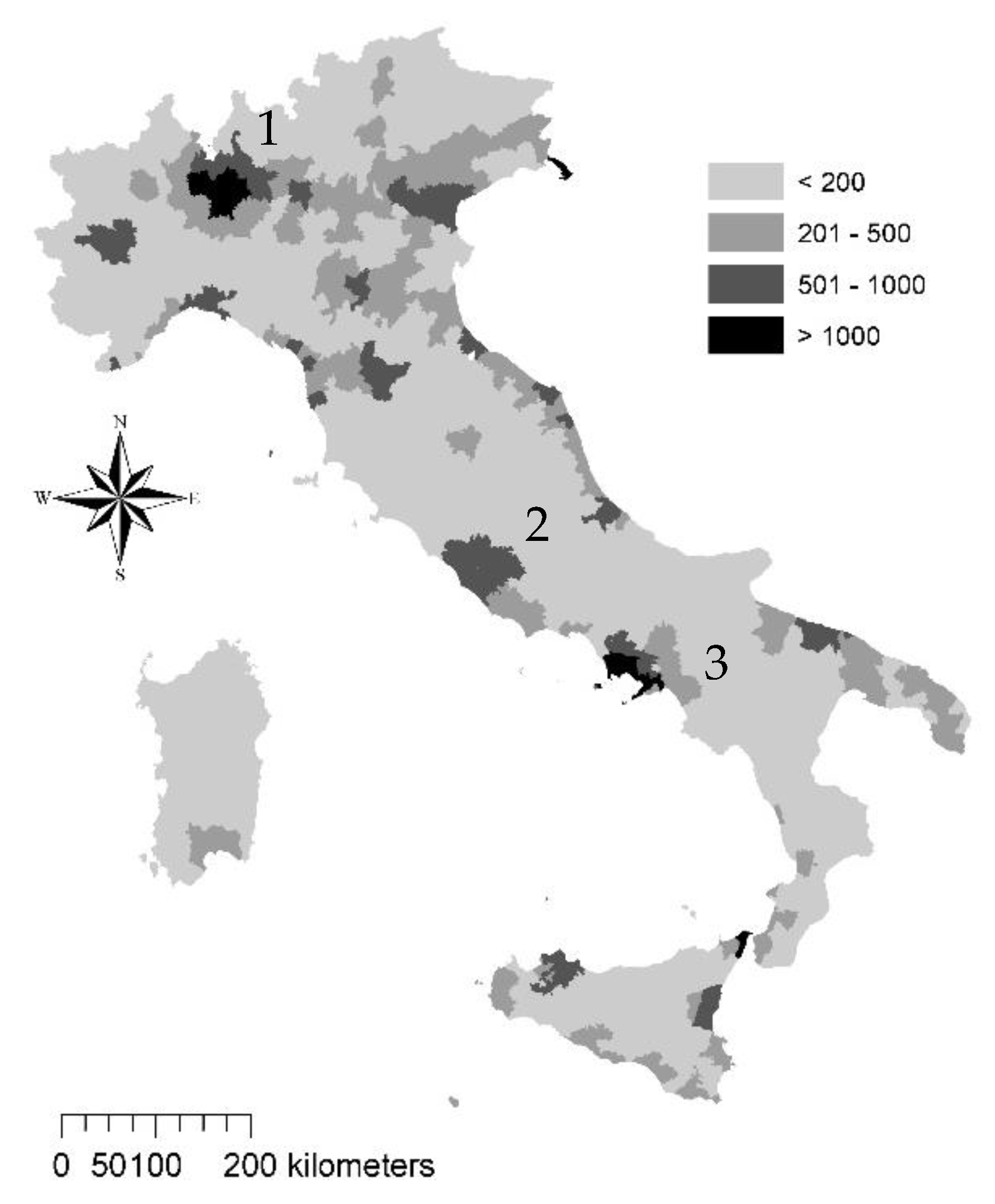This model allows the identification of urban functions related with the local market and contrasts well-organized centers with the surrounding periphery mainly devoted to the production of primary commodities, including crops and wood [46]. For instance, following the assumptions of Von Thunen’s model, the United States Bureau of Census introduced the notion of ‘Standard Metropolitan Statistical Areas’ (SMSAs), defined as urban agglomerations with a minimum population size of 200,000 inhabitants and attracting commuters from neighboring territories. In this perspective, Fujita [1] questioned the spatial organization of urban aggregates as opposed to a dispersed pattern of metropolitan growth.

Assuming cities as externality poles, they were identified as reflecting the decline in transport costs because of the proximity of markets and buyers [23]. In other words, if the market becomes more concentrated, new places devoted to the production of goods may arise in the city [2,47,48]. The functional specialization of cities implies the progressive development of economic networks and, thus, an increasing pressure on economic agent movements, modifying the spatial pattern of commuting within and between cities [31,49,50]. Considering the physical distance from central cities, [51] provided a basic theory of metropolitan growth reconnecting economic geography and urban networks, operationally focusing on the number of phones per city compared with the national average of the same variable as a proxy of urban concentration. Additional criteria were identified, for instance, in the number of economic activities or in the synergic presence of scarce services [36].

Generalizing central location theories to vastly differentiated contexts revealed to be a difficult task because commodity location factors determine (hardly predictable) conditions more (or less) favorable to industrial concentration, under the assumption that industrial location determines a concentration of labor demand [30]. At the same time, urbanization results in peripheral (settlement) growth and the abandonment of central districts, determining sequential waves of urban expansion and shrinkage [39]. Especially with rising prices of real estate, the population can be forced to move to suburban locations (e.g., [52]). In this vein, the Alonso (1968) [46] model envisages a geographical gradient in property prices extending from urban to rural locations that may be seen as an implicit indicator of centrality (e.g., [53]).

Marshall (2009) [54] identified the comparative advantage of central locations in the ability to exploit scale economies. The advantages in proximity locations intended as agglomeration economies concentrated in the Central Business Districts [55]. At the same time, urban size and centrality strictly depend on historical factors and geomorphological aspects, being in turn a function of both area and population [56]. To this end, urban centrality was investigated as a result of morphology (e.g., settlement compactness), using refined assessment techniques that assume compact settlements as central settlements as opposed to dispersed settlements typical of the periphery [35,42,57]. Assuming local economic systems as an outcome of the locational choice of businesses [37], Weber’s model of the optimal location of enterprises provided an additional framework to investigate centrality, because—as it is evident throughout historyresidential centers develop where raw materials are concentrated [13,58,59]. Zipf’s rank-size theory inspired alternative approaches based on a spatially explicit analysis of the potential imbalance between resident population and employees [60,61,62].

While explaining—often in a simplified way—the notion of centrality, urban studies and regional science considered commuting patterns and travel choices as ancillary indicator characteristics of central (or peripheral) locations [26]. Assuming the complementarity of places, Ullman (1941) [63] proposed a theory of displacement based on spatial economic differences, considering ‘territorial imbalances’ (identified as the lack of a specific function, such as population or economic activities) as an indicator of centrality (or peripherality). Implying Ullman’s place complementarity [36], the spatial gap between housing market prices and income levels was therefore seen at the base of intensified commuting patterns between the suburbs and central cities [26]. In other words, Ullman (1980) [64] envisages a block city with specialized functions and, consequently, an evident spatial segregation of different urban [17]. The presence of some services in certain locations of the city implies consumer mobility, e.g., to central locations [28]).

As a result, the radial consolidation of a network between economic centers of different importance stimulates the formation of ‘edge cities’ [65]. Interpreting cities as a part of a more complex socioeconomic system implies different (geographical and functional) levels of analysis [66]. Within this theoretical frame, it is difficult to develop a unique indicator of centrality explaining spatial differences at a very local scale [10]. For instance, population density, one of the most diffused indicators of urban centrality, failed in the joint description of residential concentration and commuting hotspots [67], confirming accessibility as a centrality factor, as in the seminal view of Ullman (1941). To this end, commuting represents the demand for cities in the sense understood by Ullman, as the need to reach a place to fulfil a given demand for work or study [46].

3. Methodology

3.1. Study Area

Covering nearly 301,330 km² of mainland, Italy is partitioned into three geographical regions (North, Center, and South) and 20 administrative regions [56] reflecting significant disparities as far as socioeconomic development is concerned [68]. Southern Italy was regarded as an economically disadvantaged district with an increasing decline after decades of continuous population growth because of the positive natural balance (number of births systematically higher than the number of deaths). Northern Italy, considered one of the wealthiest regions in continental Europe, attracted people from both Southern Italy and abroad [35]. These features make Italy a paradigmatic example of advanced economies with important within-country disparities [69]. As in other Mediterranean countries [70], the urban–rural divide in Italy was particularly accentuated [71], delineating different socioeconomic contexts from large metropolitan areas (Rome, Milan, and Naples) to hyper-rural areas (Figure 1) along the Apennine mountain chain in Central–Southern Italy [72].

A marked heterogeneity was observed in the settlement morphology and urban structures [39]. Large cities reflect both strictly monocentric and mixed settlement models; for instance, the Milan region is included in a broader polycentric network of urban centers, despite downtown Milan still acting as a monocentric model at the local scale because of the inherent density of economic activities [34]. The Naples region is basically mixed, having a particularly compact and dense central pole surrounded by satellite cities with intermediate densities [73]. Depending on the observation spatial scale, Rome was both envisaged as a polycentric city at the local scale, having more physical centers within the same municipality—the largest in Europe as far as total surface area is concerned [39]—and as a monocentric city at the regional scale, reflecting the inherent attractiveness of the Italian capital city on the surrounding districts [28]. The Alps and Apennines extend through the largest part of the Italian region, leaving few spaces to flat (or gently steep) land [69]. Apart from some port facilities, structural lacks in a modern system of railways and highways and a spatially fragmented network of airports, limited the accessibility to Southern Italy and the major islands [74]. Conversely, thanks to a flat land structure constituting a large part of Northern Italy, this region developed continuously over the last century [75], concentrating high-value activities and competitive businesses [44].

3.2. A Global Classification of Human Settlements in Italy According to the Centrality Degree

Istat has preliminary classified the Italian territory based on three levels of centrality (distinguishing ‘attractive’ and ‘intermediate’ from ‘peripheral’ locations), considering service availability/concentration and comparing the results at different spatial scales using geographical aggregates, such as local labor systems, municipalities, and submunicipal districts in major agglomerations [18]. According to this classification, the percent share of the population living in central areas at the last population census (2011) resulted to be rather low, because 84.5% of the Italian population resided in a census section classified as ‘peripheral’. However, commuting to central areas revealed to be a widespread phenomenon in Italy, and the centrality index reflects the in–out commuting ratio, calculated dividing the total flow of the population entering a given place by the flow of the population leaving the place for work or study [39]. The share of people in peripheral areas, i.e., residing in locations with a centrality index < 1, was calculated on the base of the criteria elaborated by the Parliamentary Commission. Official statistics were released at the administrative regional level, as reported in

Table 1. Spatial distribution of resident population in Italy by region and centrality level based on the original ISTAT index of centrality (Section 3.2).

Region	Total Population (Inhabitants)				Share of Resident Population (%)
	Attractive	Intermediate	Peripheral	Total	Attractive	Intermediate	Peripheral
Piedmont	410,564	294,274	3,659,078	4,363,916	9.41	6.74	83.85
Aosta Valley	10,705	6300	109,801	126,806	8.44	4.97	86.59
Lombardy	870,149	617,286	8,216,716	9,704,151	8.97	6.36	84.67
Trentino Alto Adige	104,886	62,742	861,847	1,029,475	10.19	6.09	83.72
Veneto	499,629	329,853	4,027,728	4,857,210	10.29	6.79	82.92
Friuli Venezia Giulia	128,922	74,857	1,015,206	1,218,985	10.58	6.14	83.28
Liguria	161,888	106,779	1,302,027	1,570,694	10.31	6.8	82.9
Emilia Romagna	443,848	248,224	3,650,063	4,342,135	10.22	5.72	84.06
Tuscany	323,578	226,413	3,122,211	3,672,202	8.81	6.17	85.02
Umbria	90,655	52,123	741,490	884,268	10.25	5.89	83.85
Marche	145,671	98,270	1,297,378	1,541,319	9.45	6.38	84.17
Latium	525,450	303,875	4,673,561	5,502,886	9.55	5.52	84.93
Abruzzo	128,580	85,320	1,093,409	1,307,309	9.84	6.53	83.64
Molise	29,892	24,492	259,276	313,660	9.53	7.81	82.66
Campania	541,932	340,356	4,884,522	5,766,810	9.4	5.9	84.7
Apulia	375,897	232,586	3,444,083	4,052,566	9.28	5.74	84.99
Basilicata	51,971	37,501	488,564	578,036	8.99	6.49	84.52
Calabria	149,610	96,961	712,479	1,959,050	7.64	4.95	87.41
Sicily	464,517	299,273	4,239,114	5,002,904	9.28	5.98	84.73
Sardinia	123,113	100,576	1,415,673	1,639,362	7.51	6.14	86.36
Italy	5,581,457	3,638,061	50,214,226	59,433,744	9.39	6.12	84.49

.

3.3. A Local Classification of Human Settlements in Italy Based on Commuting

The settlement classification proposed in Section 3.2 and routinely applied in official statistics at the national level, resulted in a centrality index related closely to the population distribution over space and varying with the geographical resolution of the input data [26]. Following the procedure developed by Istat (Section 3.2), the index was originally calculated at the municipal scale with relevant values—taken as official statistics—released by Istat at a lower spatial resolution, e.g., local labor systems [44]. In this way, the index delineates metropolitan regions as invariably formed by a central node surrounded by several satellite towns (Figure 2), likely demising any type of spatial heterogeneity and possibly biasing the identification of central locations and the operational delimitation of central districts at a refined spatial resolution [76]. With this perspective in mind, moving from municipalities to more detailed and disaggregated spatial units (such as the enumeration districts in use for population censuses) was demonstrated to assure a better definition of the phenomenon under consideration—making the assessment of centrality and peripherality a truly spatially explicit issue [16,21,43].

While maintaining the national coverage, the present works generalized the approach described in Section 3.2 at the enumeration district level (more than 400,000 units for Italy) with the aim of emphasizing the local dimension of urban centrality, highlighting changes in the spatial distribution of the population as far as residence and job place are jointly concerned [10]. When working with enumeration district data, however, values of centrality and peripherality cannot have the same meaning in the different socioeconomic context characteristics of countries with an intimately complex geography, as illustrated above in Section 3.1 for Italy. For instance, in a region with prevalently rural conditions, a central location can be associated with an index score slightly above 1, a value that corresponds with a noncentral location in an intermediate territory with high accessibility and specialization, e.g., in agricultural production and manufacturing [44]. Additionally, based on the spatial scale adopted in the present exercise, it is hard to say that an individual enumeration district can represent a central location tout court, because this spatial domain basically corresponds to a small part of a city (e.g., urban neighborhoods).

Based on these premises, our methodology was devoted to automatize the identification of central and peripheral districts giving an explicit value to the spatial structure of commuting patterns [26,37,42]. A spatially explicit analysis of commuting flows based on Local Indicators of Spatial Association (LISA) techniques was adopted to partition the studied territory into homogeneous clusters with specific characteristics, e.g., index values systematically high or low [77]. The application of this methodology made it possible to evaluate the intrinsic polarization of a sufficiently large spatial coverage (e.g., a continent, a country, or a broad regional entity) based on commuting patterns, i.e., investigating the spatial balance—or imbalance—of inflows and outflows [2]. A polarized area means a series of locations with systematically positive and negative values of the index, acting respectively as a sink and a source of commuting flows [34].

Unpolarized areas (basically a balanced territory as far as commuting patterns are concerned) cannot be considered as central or peripheral and thus can be defined as ‘intermediate’ [31]. Distortions could arise from the fact that enumeration districts are usually unequal in size and population density. For instance, downtown census sections resulted to be very small while those located in rural areas can reach sizes of several square kilometers. These issues could affect the outcome of spatial clustering [78] leading to issues, such as the Modifiable Area Unit Problem (MAUP). However, the local Moran approach produces a classification of areas based on the mean value of the target distribution, distinguishing different types of clusters [79]. In combination with the use of economically homogeneous areas, such as the enumeration districts [80], LISA may contain the impact of MAUP on statistical outcomes [81]. With this perspective in mind, the use of LISA based on, e.g., local Moran’s spatial autocorrelation indexes, delineated an appropriate clustering of similar (contiguous) enumeration districts [82]. The use of local Moran’s indexes assures the identification of spatial clusters calibrated finely and tuned with the intrinsic characteristics of the local context [28] and not directly associated with a predetermined threshold value of the index [39], i.e., a priori selected and valid for the whole country area [26].

Calculating a Polarization Index at the Enumeration District Level

Starting from the original formulation of the Istat centrality index (Section 3.2), a polarization index was calculated here as follows:

$$Pol\left(i,t\right)=\log \left(\frac{enter\left(i,t\right)}{s\left(i\right)}\right)-\log \left(\frac{exit\left(i,t\right)}{s\left(i\right)}\right)$$

(1)

where Pol(i,t) is the value of the polarization index at a given i-th spatial unit and time, enter(i,t) and exit(i,t) are the total inflows and outflows at the given i-th spatial unit and time, and s(i) is a specific (standardization) attribute of each spatial unit. In the specific case, the attribute coincided with the total population at the given i-th spatial unit and time. However, differential attributes could be used for standardization purposes, e.g., the surface area of the given i-th spatial unit. Logarithmic transformation was implemented here to better manage casual heterogeneity in variation ranges. Given the broad heterogeneity of the enumeration districts, few cases arose of districts where people only work (i.e., pure business districts with no residences). Zero residents mean that a net population inflow was recorded in such units [18]. While this issue never arose at the municipal level (i.e., the spatial unit of the original Istat procedure), in the present study, we applied a scale transformation adding 1 to both inflows (enter) and outflows (exit) to avoid a null argument.

An additional issue stems from the fact that Pol(i,t) index values are not necessarily in line with a priori benchmarks (based, e.g., on economic, demographic, statistical, or planning rules). For instance, the grand average of the statistical distribution of Pol(i,t) can be different from 0, which is the target value indicating a balanced spatial structure with an equal amount of inflows and outflows. This suggests a generalization of the procedure distinguishing central areas (where the commuting ratio is positive) from peripheral areas (where the ratio is negative) by using the Pol(i,t) grand mean as the reference value. To address such aspects, we translated the polarization index using a linear transformation, as follows:

$$Pol\left(i,t\right) *=Pol\left(i,t\right)-\mathrm{E}\left[Pol\left(i,t\right)\right]$$

(2)

where E[Pol(i,t)] is the grand average of all values of the polarization index measured all over the country. Following Equation (2) applied to the 2011 population census data, Pol(i,t) * assumed for Italy an average value of 0.207 with a standard deviation amounting to 1.478 (n = 402,677 enumeration districts), showing in turn a non-significant spatial structure at the global level, with a Moran I spatial autocorrelation coefficient equal to 0.14 (p > 0.01).

3.4. The Spatial Outcome of a Polarization Index Based on LISA Clustering

Taken as the base of a spatially explicit evaluation of central (i.e., attractive) and peripheral (i.e., repulsive) clusters, the evaluation of spatial autocorrelation regimes in the Pol(I,t) * index described above was carried out using Moran’s coefficients, which calculate spatial autocorrelation based on feature positions and values at the same time [78]. Moran’s global and local indexes of spatial autocorrelation were calculated to estimate spatial dependency based on scatterplots [26]. The global Moran index was run adopting a sufficiently small distance range (10 km) compatible with the geometry of the enumeration districts, producing z-scores with statistically significant levels for spatial autocorrelation at p < 0.05 [28]). Global Moran’s autocorrelation indexes allow evaluating the degree of association between the observed values and the spatially weighted averages of neighboring values [83,84,85], using a contiguity spatial matrix assumed as the most relevant representation of the spatial relationship for commuting inflows and outflows.

The local Moran’s indexes were finally run with the aim of assessing spatial dependence in any subarea of the country. This approach identifies spatial clustering of similar (or different) values [78]. A positive value of the local Moran’s index describes spatial clustering of similar (high or low) values between a given district and its neighbors. A negative value in turn indicates spatial clustering of dissimilar values [39]. Local Moran’s homogeneous clusters of Pol(i,t) * positive values were intended as central locations. Clusters were associated with a probability level indicating the statistical significance of a territorial partition. This probability level allowed partitioning enumeration districts into five classes (HH: clusters with systematically high (i.e., statistically significant) index values, namely ‘central’ places; HL: clusters with index values under spatial transition from high values to low values, namely ‘central– intermediate’ places; LH: low–high clusters, with index values under spatial transition from low values to high values, namely ‘intermediate–peripheral’ places; LL: clusters with systematically low index values, namely ‘peripheral’ places; and, finally, unclustered areas with indistinct and unpolarized patterns from the ‘in–out commuting flow’ perspective.

Considering their specific characteristics, HH and LL clusters were respectively associated with central and peripheral locations, reflecting the intrinsic polarization in source and sink territories typical (but not exclusive) of metropolitan agglomerations and more dynamic rural (accessible) areas [75]. HL and LH were regarded as transitional areas with more balanced commuting patterns, assumed to be located, e.g., at the fringe of central locations [35]. Insignificant clusters of enumeration districts finally indicate the balanced and unpolarized territory typical of intermediate rural areas with medium–low population density mostly organized in small villages and isolated settlement nuclei [14].

An indirect analysis of the result stability was finally carried out comparing the outcomes of the procedure under five iterative solutions, i.e., based on a Queen spatial matrix with varying contiguity orders from 1 to 5 [80]. This exercise allows exploring different spatial settings and relationships, moving from a strictly local scale (contiguity order 1)—particularly appropriate to investigate centrality in urban areas under very small spatial units—to a broader scale (contiguity order 5) appropriate to identify peripherality in rural areas with supposedly bigger enumeration districts [39]. In this way, we intrinsically controlled for the size of the enumeration [18], in turn providing an indirect validation of the final outcomes of the methodology [78]. The stability of the outcomes with increasing contiguity order was taken as evidence of the overall reliability and internal coherence of the settlement classification [28]). The stability of the outcomes was checked calculating the average value of Pol(i,t) * by local Moran’s clustering classification (HH, HL, LH, and LL) and contiguity orders from 1 to 5 [26].

3.5. Testing the Spatial Stability of the Index with Geographically Weighted Regression (GWR)

As stated above, working with heterogeneous spatial domains, such as the enumeration districts, implies the existence of the Modifiable Area Unit Problem (MAUP). This issue regards the possible impact of the individual spatial unit size on the final estimation of the target variable, namely the polarization index. In an effort to verify the internal coherence and spatial stability of this index [37], we addressed the MAUP with an empirical approach verifying the intrinsic relationship between the polarization index value at the enumeration district scale and the total size (ha) of the elementary analysis of the spatial units. The empirical test of this correlation is a particularly important issue not only for the MAUP, but also for the internal verification of the Pol(i,t) * stability in urban and rural contexts [17]. As a matter of fact, enumeration districts are, for construction, smaller in urban areas and larger in rural areas, and this is particularly evident in the Italian geography.

In this context, we assumed local regressions as documenting significant (or nonsignificant) relationships between local index values and the size (i.e., surface area) of each district. A nonsignificant relationship between the local Pol(i,t) * and the surface area of enumeration districts suggest that (i) MAUP is an irrelevant problem in the data sample analyzed here at the specified spatial scale and (ii) the spatial distribution of the local polarization index is comparable in urban and rural areas (i.e., between larger and smaller districts). When testing the abovementioned relationship, a local regression approach was considered more effective than a global regression model because it takes account of the spatial structure of the variables at stake (both the dependent variable and the predictor), in turn providing a local estimate of the adjusted R² and regression coefficients [28]).

This approach was operationalized by adopting a Geographically Weighted Regression (GWR) strategy [86]. Keeping the spatial structure explicit, this approach evaluated the impact of a predictor (surface area of each enumeration district) on the polarization index at the same spatial scale [87]. The model’s goodness of fit was assessed using (global and local) the R² coefficients and t-statistics testing for significant regression coefficients at p < 0.01. The impact of the predictor on the dependent variable was estimated using a linear model run on standardized data [26]). By adopting a kernel function to calculate the weights for the estimation of the local models, GWRs identify local-scale variability in population dynamics [88]. The methodological framework characteristic of a GWR is similar to that of local regression models; contrary to a spatially implicit ordinary least square regression (i.e., with location invariant regression coefficients), a GWR runs an econometric specification for each location s = 1, …, n, as follows:

Y(s) = X(s)B(s) + e(s)

(3)

where Y(s) is the dependent variable at location s (i.e., polarization index value), X(s) includes the selected predictor (i.e., surface area of each enumeration district) at location s, B(s) includes the regression coefficients, and e(s) is the random error, all being calculated at location s. As a result, the GWR gave rise to a distribution of local estimated parameters, namely local slope coefficients and local intercepts [28]. A bi-square nearest neighbor kernel function [76] was the weighting scheme adopted in this study. Based on these premises, we tested for (i) non-significant (p > 0.01) locally adjusted R² and (ii) non-significant local slope coefficients. These outcomes reflected spatial stability and internal coherence of the polarization index following the experimental assumptions presented above. On the contrary, we expected local intercepts equal to or different from zero, because they capture the local heterogeneity of the dependent variable (polarization index) irrespective of the impact of the predictor (size of enumeration districts).

4. Results

Table 2. Average value of the polarization index at the enumeration district scale by spatial clustering classification (HH: high–high, LL: low–low; LH: low–high; and HL: high–low).

Contiguity Order	HH	HL	Insignificant	LH	LL
1	4.76	1.28	0.65	0.26	0.16
2	3.65	1.51	0.64	0.26	0.18
3	3.22	1.58	0.65	0.25	0.19
4	2.99	1.62	0.66	0.25	0.20
5	2.82	1.63	0.67	0.25	0.20

illustrates the spatial drift of the mean value of the polarization index by enumeration district as the contiguity order increases, assuming Queen matrices of spatial contiguity (from the first to the fifth orders) as representative of the spatial structure of the enumeration districts. The empirical data show how, as the order of contiguity varies, the mean values of the polarization index associated with the HH and HL clusters change as a linear function of the contiguity order. In particular, the average values associated with the central clusters HH decrease linearly with the increase in the contiguity order, while the average values associated with the transitional clusters HL follow the reverse pattern, rising weakly with the increase in the order of contiguity and reaching a plateau with the orders 4 and 5. However, considering the HH and HL clusters together, i.e., assuming a classification of centrality extended to transitional territories, the mean polarization index tends to stabilize around values of 2.5 as the contiguity order increases, with modest differences among contiguity orders. All the other territorial partitions deriving from the classification of the enumeration districts showed particularly stable mean values of the polarization index as the contiguity order varies.

4.1. Spatial Clustering

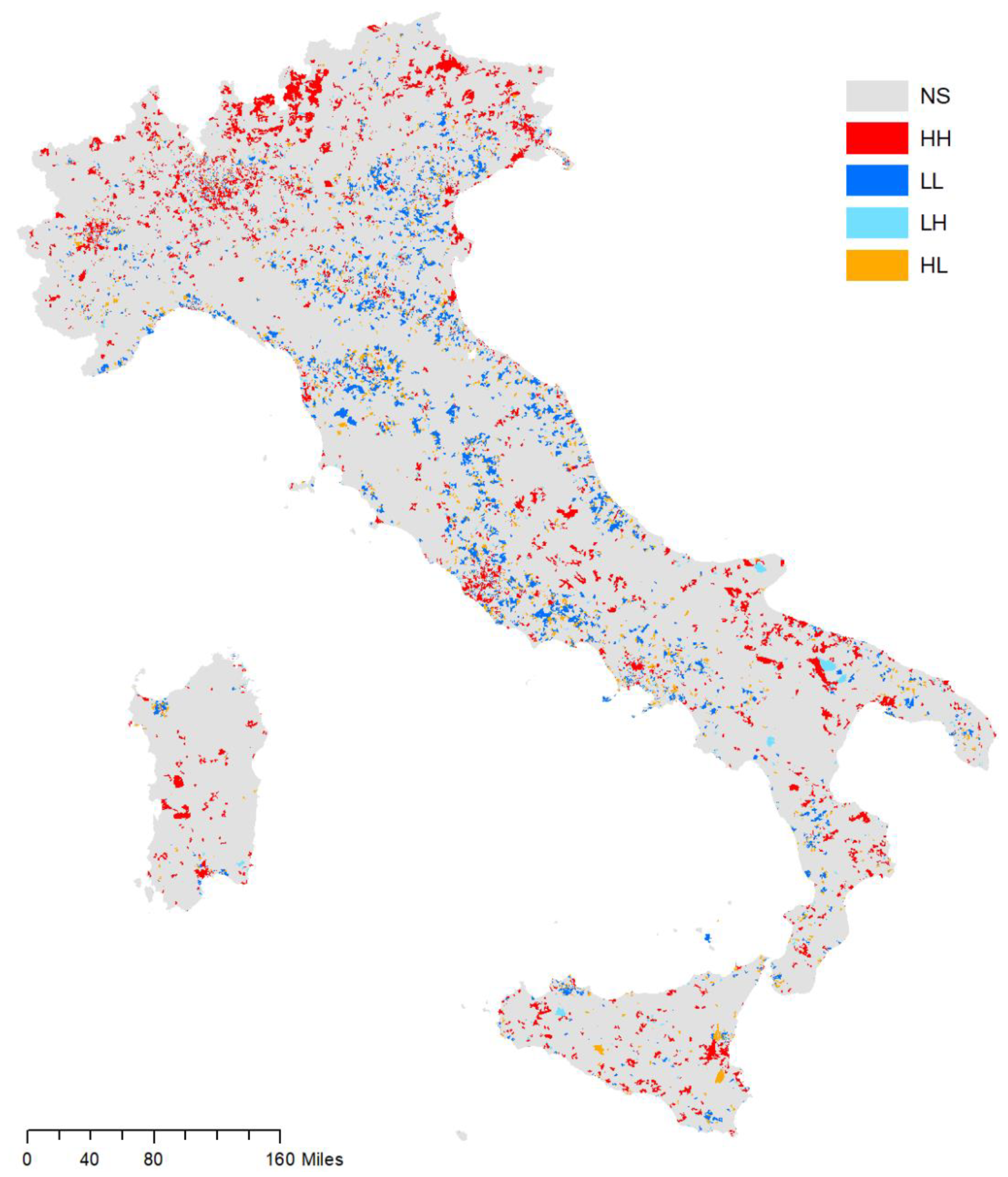
The enumeration districts classified with an insignificant spatial structure (i.e., unpolarized from the point of view of commuting patterns) have values of the polarization index systematically lower than unity (0.64–0.67), thus indicating a weak drift toward economic marginality (about 65 incoming workers out of 100 outcoming workers, on average). These values resulted to be stable as a function of the contiguity order, indicating that the definition of polarized space deriving from LISA was not influenced by the spatial neighborhood. The enumeration districts classified as ‘peripheral’ (LL clusters) had an average polarization index close to 0.2. This means that, in such locations, the inflow of commuters was systematically lower than the outflow (on average 20 workers entered for 100 workers who left the place), thus reflecting the ‘economic repulsion’ of such territories regardless of the structure of the spatial environment; in other words, the average polarization index remained completely stable as the contiguity order varied. Finally, the transitional enumeration districts classified as ‘intermediate-peripheral’ (LH clusters) showed equally stable mean values of the polarization index that ranged between 0.25 and 0.26, evidencing economically marginal territories where, on average, 25 workers entered out of 100 who left.

Figure 3 illustrates an example of the classification of the Italian territory based on LISA clustering of the polarization index, considering an order of spatial contiguity of the Queen matrix equal to 1. Most of the Italian territory was classified as nonpolarized, in line with the underlying assumptions of the index. These territories coincide with an intermediate economic space, both in mountainous areas and in the most accessible places. On the contrary, the greatest level of polarization was observed in coastal areas and in flat inland areas with greater infrastructural development. Central clusters concentrated in metropolitan areas and basically revealed their fine-scale geography using enumeration districts. Peripheral clusters were more scattered throughout the Italian territory being close to metropolitan areas and functionally linked to central areas. A small number of peripheral clusters, however, were geographically more remote, i.e., belonging to more marginal districts from an economic point of view. This spatial pattern reflects the geographical outcomes deriving from short-range and medium-range mobility patterns.

4.2. Descriptive Statistics of the Polarization Index

The statistical distribution of the enumeration districts (frequency, total population, and land size) is illustrated in

Table 3. The number of enumeration districts, total population, and surface area therein, by spatial clustering and contiguity order.

Contiguity Order	Insignificant	Absolute Number				Insignificant	Index Number (Cont.Order 1 = 100)
		HH	LL	LH	HL		HH	LL	LH	HL
Enumeration district (number)
1	322,032	33,199	25,910	7995	13,276	100.0	100.0	100.0	100.0	100.0
2	272,794	49,100	39,520	16,115	24,883	84.7	147.9	152.5	201.6	187.4
3	228,474	64,002	49,280	24,274	36,382	70.9	192.8	190.2	303.6	274.0
4	195,686	73,232	56,707	30,925	45,862	60.8	220.6	218.9	386.8	345.4
5	172,524	78,642	61,922	35,773	53,551	53.6	236.9	239.0	447.4	403.4
Total population (1000 inhabitants)
1	47,259	2327	6387	1899	1562	100.0	100.0	100.0	100.0	100.0
2	40,074	3513	9050	4032	2764	84.8	150.9	141.7	212.4	177.0
3	34,241	4243	11,343	5842	3765	72.5	182.3	177.6	307.7	241.1
4	29,559	4722	13,290	7184	4679	62.5	202.9	208.1	378.4	299.6
5	25,901	5051	14,805	8201	5476	54.8	217.0	231.8	432.0	350.6
Surface area (km2)
1	26.573	1.717	1.116	247	550	100.0	100.0	100.0	100.0	100.0
2	22.565	4.069	1.924	522	1.123	84.9	237.0	172.5	211.2	204.2
3	18.409	6.562	2.521	830	1.880	69.3	382.2	226.0	336.2	341.8
4	15.915	7.660	2.996	1.071	2.560	59.9	446.1	268.6	433.7	465.5
5	14.184	8.242	3.368	1.260	3.149	53.4	480.0	301.9	510.2	572.5

. The results of the descriptive analysis indicate, as expected, that the number of central areas corresponding with the HH clusters of the neighboring districts (i.e., characterized by systematically high values of the polarization index) was relatively low (33 thousands), more than doubling when moving from the first order to the fifth order Queen contiguity spatial matrix. This pattern was in line with the reduction in the average polarization index shown in Table 2.

The increase in the polarization index characteristic of the HH clusters was associated with a progressive decrease in the number of enumeration districts classified as HH clusters. Based on these results, it seems not appropriate to select an a priori level of centrality, assuming it as a function of the contiguity order. In the exploratory context characteristic of our approach, a specific level of centrality finely tuned with the geography of the polarization index can be selected or, alternatively, a linear function that links the level of centrality with the contiguity order can be defined, e.g., by comparing different spatial configurations of LISA at varying contiguity orders.

4.3. Geographically Weighted Regression

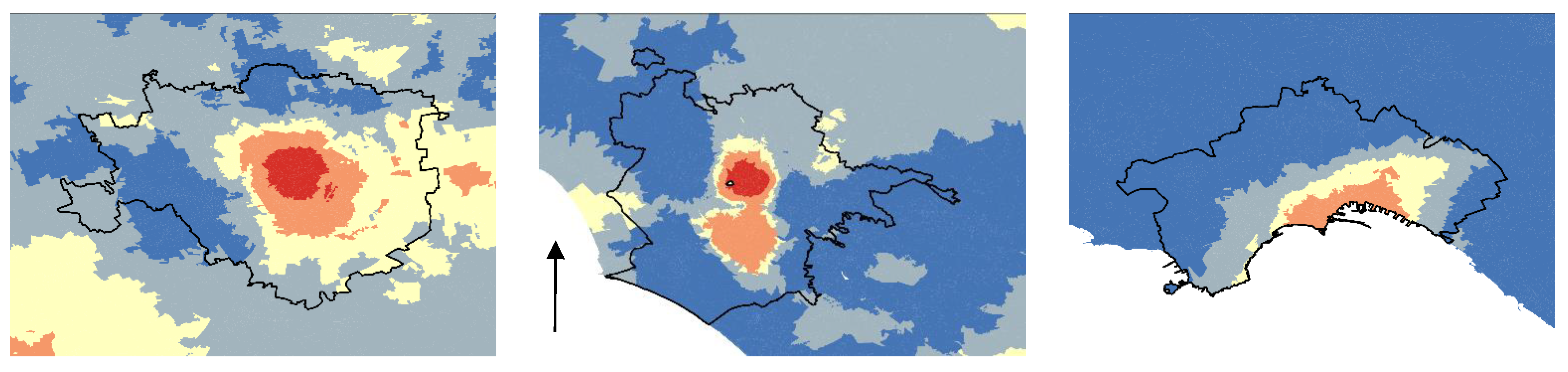
The results of the GWR indicate a negligible effect of the enumeration district size as a predictor of the polarization index (global adjusted R² = 0.05), with the local R² and local slope coefficients close to zero (p > 0.05). These findings suggest the validity of the working hypothesis (i.e., the null impact of the predictor on the dependent variable) and confirm (i) the inexistence (or the nonrelevance) of the MAUP effects at the investigated spatial scale and (ii) the substantial stability of the polarization index across the different typologies of the enumeration districts (e.g., rural vs. urban). An indirect confirmation of this assumption came from the spatial distribution of the standardized local intercepts, indicating spatial heterogeneity irrespective of the predictor’s impact. The spatial distribution of the standardized local intercepts in the three exemplificative landscape scenes (i.e., the metropolitan regions of Milan, Rome, and Naples—the three largest cities in Italy) are illustrated in Figure 4. These maps delineate positive and significant values of the local intercept in correspondence with the three cities (Milan, Rome, and Naples), indirectly delineating central locations irrespective of the size of the enumeration districts and confirming the spatial stability and internal coherence of the polarization index.

5. Discussion

In recent times, the notion of central locations was broadly debated under different disciplinary perspectives—from urban geography and spatial planning to regional economics and rural sociology—often becoming a cross-cutting issue in between research and policy [36]. The consensus is still limited on the operational delimitation of cities and metropolitan regions [30]. More importantly, there is a different definition of the administrative boundaries of a city and its effective integration into a broader area. Intensively urbanized areas may transcend the administrative boundaries and should be considered as individual cities despite their administrative/governance settings [39]. The operational delimitation of centers and suburbs that takes part in (more or less) articulated city networks at different spatial scales was regarded as another complex task [42].

Intended as central locations, places that are most successful in attracting people require transportation infrastructure and services to meet the expanding demand of the resident population [46]. Following this rationale, the locations from which people leave daily moving to work are assumed as urban centralities [13]. There are several strands of literature dealing with urban centrality, the first focusing on the physical definition and delimitation of central locations and the second addressing the phenomenology and manifestation of negative and positive (economic) externalities [32]. In this regard, the main issues examined in the recent literature concern transport efficiency [89], pollution [90], and energy efficiency [91].

Different methodologies delineating the central and peripheral areas are the result of vastly different analysis solutions investigating the presence of services and the extent of market areas, basically referring to the Christaller and Losch theories of the spatial localization of industries [41]. A generalization of these approaches allows a refined analysis of the complex system of relationships among urban centers, giving room to an operational discrimination of monocentric or polycentric models reflecting regional settlement structures or the characteristics of specific local development paths [18]. Accordingly, the position (or status) of a central location in a given urban network is a function of the physical distance or, more generally, depends on the spatial structure of the neighbors [26].The identification of different settlement types thus implies the estimation of a metric discriminating central from peripheral locations (and, possibly, the intermediate space in between) as a function of physical distance or the intrinsic spatial structure [92].

In this line of thinking, the present work investigated commuting patterns at a submunicipal level (enumeration district) providing a novel (functional) approach to centrality and periphery [37], being inspired by an official statistics experience (held by the Italian National Statistical Institute, Istat) that responded to a normative design and pressing demand for territorial indicators. Considering commuting patterns, this analysis indirectly focuses on patterns and processes of local development [21]. To address such issues, our approach runs a spatial clustering of a polarization index quantifying home-to-work daily travels [92]. The procedure delineates submunicipal (homogeneous) areas (bigger than enumeration districts) that are considered sinks (centers) or sources (peripheries) of commuter flows [31].

Taken together, these results demonstrate how the choice of the spatial neighborhood (contiguity order) did not affect the functional classification of a given territory deriving from the analysis of LISA spatial clusters. This is always true in our data with the sole exception of central locations (corresponding with HH clusters) and, in part, of ‘transitional’ central–intermediate locations (HL clusters). The identification of these specific territorial aggregations (HH and HL clusters) depends on the contiguity order chosen within the spatial matrix adopted for computation [52]). Higher contiguity orders include districts with a low average level of centrality and, conversely, delineate extended central areas. The approach proposed in this work, therefore, highlights how the definition of peripheral, peripheral in transition, and nonpolarized territories is not influenced by the spatial neighborhood and therefore does not depend on the function associated with the geographical matrix used in the LISA analysis [80].

These findings indirectly document the internal stability of the territorial partition and the reliability of the polarization index, confirming the goodness of representation and the internal coherence of the chosen observation scale [93]. On the contrary, the level of centrality seems to depend on the structure of the spatial environment, reflecting a greater polarization associated with territorial [26]. Therefore, the identification of central areas needs to fix a priori an average level of centrality or, alternatively, to study the variability of this measure as a function of different spatial structures [23], as proposed in this work. These results suggest the importance of modeling complex indicators of centrality as a function of both their dependence on the global spatial scale and on the local structure of the spatial neighborhood [29].

The appropriateness of using commuter flows as a basic indicator of spatial polarization that reflects both central and peripheral locations is finally documented in a vast number of earlier studies in the field of official statistics—only partly referring to the central location theory [94]. Commuting was widely investigated to identify socioeconomic processes oriented along (and influenced by) the center–periphery gradient [95]. In an attempt to delineate Functional Urban Areas (FUAs) taken as a relevant spatial domain, peripheral districts of high-density clusters were identified on the basis of the percent share of workers commuting into this district of the total commuters [96,97,98]. Core districts were identified as a cluster of neighbor spatial partitions with population densities above 1500 inhabitants [99,100,101]. The definitions of Inland Areas operationally adopted in official statistics (and variably developed by European governments as a tool for defining central and marginal areas as a function of accessibility) follow the same rationale [12,102,103].

For instance, the operational definition of travel to work areas, or local labor systems—an important spatial aggregate in official statistics—also derived from these assumptions and practical issues [44]. One of the first empirical applications to identify local labor systems in Italy dated back to the 1980s when, likely for the first time in continental Europe—apart from the exception of the United Kingdom—they were derived from a commuting matrix using microdata from population censuses [96,104,105]. This exercise also identified core cities together with the related urban hierarchy at a broader spatial scale [35]. Core cities were assumed as the center of human activities, a development node distinctive from the surrounding periphery [16]. Taken as a dominant factor in economic development [41], accessibility and, consequently, commuting patterns thus became a key to operationally define functional areas [38].

6. Conclusions

The purpose of our analysis was to show that the centrality index proposed by the Italian Parliamentary Commission may have some operational pitfalls at small spatial scales (i.e., with high-resolution data). In fact, the municipal figures of this index represent an ‘average’ socioeconomic context deriving from heterogeneous socioeconomic outcomes at the local scale. The use of more detailed observation scales (e.g., enumeration districts) imposes a modification of the index, moving to a spatially explicit approach to economic polarization. However, if the practical use of such indexes at the municipal (or coarser) scales is difficult because of the spatial variability, an extensive use at smaller scales is also problematic because of the intrinsic fragmentation of the economic space. The LISA approach represents an interesting compromise allowing the definition of spatial clusters with homogeneous values of the polarization index derived from a process of spatial addition of neighboring districts. Looking at the LISA clusters (basically the HH and LL clusters) provides a dynamic view of local (i.e., municipal and submunicipal) centralities and peripheries. By defining the true geography of the central and peripheral locations at the local scale and a more coherent spatial pattern at the national scale, this approach provides a comprehensive framework for the analysis of population, settlement, and mobility demand. See Appendix A.

References

1. Fujita, M. Spatial patterns of urban growth: Optimum and market. J. Urban Econ. 1976, 3, 209–241. [Google Scholar] [CrossRef]
2. Egan, D.J.; Nield, K. Towards a Theory of Intraurban Hotel Location. Urban Stud. 2000, 37, 611–621. [Google Scholar] [CrossRef]
3. Castells, M. Livable Cities? Urban Struggles for Livelihood and Sustainability; University of California Press: San Francisco, CA, USA, 2002. [Google Scholar]
4. Skog, K.L.; Steinnes, M. How do centrality, population growth and urban sprawl impact farmland conversion in Norway? Land Use Policy 2016, 59, 185–196. [Google Scholar] [CrossRef]
5. Siewwuttanagul, S.; Inohae, T.; Mishima, N. An Investigation of Urban Gravity to Develop a Better Understanding of the Urbanization Phenomenon Using Centrality Analysis on GIS Platform. Procedia Environ. Sci. 2016, 36, 191–198. [Google Scholar] [CrossRef]
6. Clark, J.; Harrison, J.; Miguelez, E. Connecting cities, revitalizing regions: The centrality of cities to regional development. Reg. Stud. 2018, 52, 1025–1028. [Google Scholar] [CrossRef]
7. Khatam, A.; Haas, O. Interrupting planetary urbanization: A view from Middle Eastern cities. Environ. Plan. D Soc. Space 2018, 36, 439–455. [Google Scholar] [CrossRef]
8. Golubchikov, O. The urbanization of transition: Ideology and the urban experience. Eurasian Geogr. Econ. 2016, 57, 607–623. [Google Scholar] [CrossRef]
9. Gomez, J.E.A., Jr. The size of cities: A synthesis of multi-disciplinary perspectives on the global megalopolis. Prog. Plan. 2017, 116, 1–29. [Google Scholar] [CrossRef]
10. Zambon, I.; Benedetti, A.; Ferrara, C.; Salvati, L. Soil Matters? A Multivariate Analysis of Socioeconomic Constraints to Urban Expansion in Mediterranean Europe. Ecol. Econ. 2018, 146, 173–183. [Google Scholar] [CrossRef]
11. Brenner, N. New urban spaces: Urban theory and the scale question. Oxford University Press: Oxford, UK, 2019. [Google Scholar]
12. Perrin, C.; Nougarèdes, B.; Sini, L.; Branduini, P.; Salvati, L. Governance changes in peri-urban farmland protection following decentralisation: A comparison between Montpellier (France) and Rome (Italy). Land Use Policy 2018, 70, 535–546. [Google Scholar] [CrossRef] [Green Version]
13. Berry, B.J.L.; Simmons, J.W.; Tennant, R.J. Urban Population Densities: Structure and Change. Geogr. Rev. 1963, 53, 389. [Google Scholar] [CrossRef]
14. Cecchini, M.; Zambon, I.; Pontrandolfi, A.; Turco, R.; Colantoni, A.; Mavrakis, A.; Salvati, L. Urban sprawl and the ‘olive’ landscape: Sustainable land management for ‘crisis’ cities. GeoJournal 2019, 84, 237–255. [Google Scholar] [CrossRef]
15. Governa, F.; Saccomani, S. From urban renewal to local development. New conceptions and governance practices in the Italian peripheries. Plan. Theory Pract. 2004, 5, 327–348. [Google Scholar] [CrossRef]
16. Duvernoy, I.; Zambon, I.; Sateriano, A.; Salvati, L. Pictures from the other side of the fringe: Urban growth and peri-urban agriculture in a post-industrial city (Toulouse, France). J. Rural. Stud. 2018, 57, 25–35. [Google Scholar] [CrossRef]
17. Di Feliciantonio, C.; Salvati, L.; Sarantakou, E.; Rontos, K. Class diversification, economic growth and urban sprawl: Evidences from a pre-crisis European city. Qual. Quant. 2018, 52, 1501–1522. [Google Scholar] [CrossRef]
18. Salvati, L.; Carlucci, M. Patterns of Sprawl: The Socioeconomic and Territorial Profile of Dispersed Urban Areas in Italy. Reg. Stud. 2016, 50, 1346–1359. [Google Scholar] [CrossRef]
19. Dow, K. Social dimensions of gradients in urban ecosystems. Urban Ecosyst. 2000, 4, 255–275. [Google Scholar] [CrossRef]
20. Fowler, C.S. Segregation as a multiscalar phenomenon and its implications for neighborhood-scale research: The case of South Seattle 1990–2010. Urban Geogr. 2015, 37, 1–25. [Google Scholar] [CrossRef] [PubMed]
21. Bayona-I-Carrasco, J.; Gil-Alonso, F.; Rubiales-Pérez, M.; Pujadas-Rúbies, I. New Spatial Mobility Patterns in Large Spanish Cities: From the Economic Boom to the Great Recession. Appl. Spat. Anal. Policy 2017, 11, 287–312. [Google Scholar] [CrossRef]
22. Cheshire, P.; Magrini, S. Endogenous Processes in European Regional Growth: Convergence and Policy. Growth Chang. 2000, 31, 455–479. [Google Scholar] [CrossRef]
23. Kombe, W.J. Land use dynamics in peri-urban areas and their implications on the urban growth and form: The case of Dar es Salaam, Tanzania. Habitat Int. 2005, 29, 113–135. [Google Scholar] [CrossRef]
24. Cheshire, P.; Magrini, S. Urban growth drivers in a Europe of sticky people and implicit boundaries. J. Econ. Geogr. 2008, 9, 85–115. [Google Scholar] [CrossRef]
25. Egidi, G.; Cividino, S.; Vinci, S.; Sateriano, A.; Salvia, R. Towards Local Forms of Sprawl: A Brief Reflection on Mediterranean Urbanization. Sustainability 2020, 12, 582. [Google Scholar] [CrossRef]
26. Ciommi, M.; Chelli, F.M.; Salvati, L. Integrating parametric and non-parametric multivariate analysis of urban growth and commuting patterns in a European metropolitan area. Qual. Quant. 2019, 53, 957–979. [Google Scholar] [CrossRef]
27. McMillen, D.P.; William Lester, T. Evolving subcenters: Employment and population densities in Chicago, 1970–2020. J. Hous. Econ. 2003, 12.1, 60–81. [Google Scholar] [CrossRef]
28. Baumont, C.; Ertur, C.; Le Gallo, J. Spatial analysis of employment and population density: The case of the agglomeration of Dijon 1999. Geogr. Anal. 2004, 36, 146–176. [Google Scholar] [CrossRef]
29. Salvati, L.; Zitti, M.; Sateriano, A. Changes in city vertical profile as an indicator of sprawl: Evidence from a Mediterranean urban region. Habitat Int. 2013, 38, 119–125. [Google Scholar] [CrossRef]
30. Capello, R.; Camagni, R. Beyond Optimal City Size: An Evaluation of Alternative Urban Growth Patterns. Urban Stud. 2000, 37, 1479–1496. [Google Scholar] [CrossRef]
31. Dietzel, C.; Herold, M.; Hemphill, J.J.; Clarke, K.C. Spatio-temporal dynamics in California’s Central Valley: Empirical links to urban theory. Int. J. Geogr. Inf. Sci. 2005, 19, 175–195. [Google Scholar] [CrossRef]
32. Cheshire, P.; Carbonaro, G. Urban Economic Growth in Europe: Testing Theory and Policy Prescriptions. Urban Stud. 1996, 33, 1111–1128. [Google Scholar] [CrossRef]
33. Jonas, A.E.; McCann, E.; Thomas, M. Urban Geography: A Critical Introduction. Wiley: London, United Kingdom, 2015. [Google Scholar]
34. Carlucci, M.; Chelli, F.M.; Salvati, L. Toward a New Cycle: Short-Term Population Dynamics, Gentrification, and Re-Urbanization of Milan (Italy). Sustainability 2018, 10, 3014. [Google Scholar] [CrossRef]
35. Ciommi, M.; Chelli, F.M.; Carlucci, M.; Salvati, L. Urban Growth and Demographic Dynamics in Southern Europe: Toward a New Statistical Approach to Regional Science. Sustainability 2018, 10, 2765. [Google Scholar] [CrossRef]
36. Capello, R. Recent Theoretical Paradigms in Urban Growth. Eur. Plan. Stud. 2013, 21, 316–333. [Google Scholar] [CrossRef]
37. Andersson, C.; Frenken, K.; Hellervik, A. A Complex Network Approach to Urban Growth. Environ. Plan. A Econ. Space 2006, 38, 1941–1964. [Google Scholar] [CrossRef]
38. Vickerman, R.; Spiekermann, K.; Wegener, M. Accessibility and Economic Development in Europe. Reg. Stud. 1999, 33, 1–15. [Google Scholar] [CrossRef]
39. Salvati, L.; Carlucci, M. A composite index of sustainable development at the local scale: Italy as a case study. Ecol. Indic. 2014, 43, 162–171. [Google Scholar] [CrossRef]
40. LaMonica, G.R.; Recchioni, M.C.; Chelli, F.M.; Salvati, L. The efficiency of the cross-entropy method when estimating the technical coefficients of input–output tables. Spat. Econ. Anal. 2020, 15, 62–91. [Google Scholar] [CrossRef]
41. Alonso, W. The Historic and the Structural Theories of Urban Form: Their Implications for Urban Renewal. Land Econ. 1964, 40, 227. [Google Scholar] [CrossRef]
42. Delloye, J.; Lemoy, R.; Caruso, G. Alonso and the Scaling of Urban Profiles. Geogr. Anal. 2019, 52, 127–154. [Google Scholar] [CrossRef]
43. Chelleri, L.; Schuetze, T.; Salvati, L. Integrating resilience with urban sustainability in neglected neighborhoods: Challenges and opportunities of transitioning to decentralized water management in Mexico City. Habitat Int. 2015, 48, 122–130. [Google Scholar] [CrossRef]
44. Recanatesi, F.; Clemente, M.; Grigoriadis, E.; Ranalli, F.; Zitti, M.; Salvati, L. A Fifty-Year Sustainability Assessment of Italian Agro-Forest Districts. Sustainability 2016, 8, 32. [Google Scholar] [CrossRef]
45. Portugali, J. Self-Organization and The City. Springer: Berlin, Germany, 1999. [Google Scholar]
46. Alonso, W. Urban and Regional Imbalances in Economic Development. Econ. Dev. Cult. Chang. 1968, 17, 1–14. [Google Scholar] [CrossRef]
47. Krugman, P. The Role of Geography in Development. Int. Reg. Sci. Rev. 1999, 22, 142–161. [Google Scholar] [CrossRef]
48. Jarosz, L. The city in the country: Growing alternative food networks in Metropolitan areas. J. Rural. Stud. 2008, 24, 231–244. [Google Scholar] [CrossRef]
49. Blanquart, C.; Koning, M. The local economic impacts of high-speed railways: Theories and facts. Eur. Transp. Res. Rev. 2017, 9, 12. [Google Scholar] [CrossRef]
50. Buck, N.; Gordon, I.R.; Harding, A. Changing Cities: Rethinking Urban Competitiveness, Cohesion and Governance; Bloomsbury: London, UK, 2017. [Google Scholar]
51. Berry, B.J.I.; Baskin, C.W.; Christaller, W. Central Places in Southern Germany. Econ. Geogr. 1967, 43, 275. [Google Scholar] [CrossRef]
52. Salvati, L.; Carlucci, M. Shaping Dimensions of Urban Complexity: The Role of Economic Structure and Socio-Demographic Local Contexts. Soc. Indic. Res. 2019, 147, 263–285. [Google Scholar] [CrossRef]
53. Clark, C. Urban population densities. J. R. Stat. Society. Ser. A 1951, 114, 490–496. [Google Scholar] [CrossRef]
54. Marshall, A. Principles of Economics: Unabridged Eighth Edition; Cosimo: New York, NY, USA, 2009. [Google Scholar]
55. Adrian, C.R. Metropology: Folklore and field research. JSTOR 1961, 21, 148–157. [Google Scholar] [CrossRef]
56. Bajocco, S.; Ceccarelli, T.; Smiraglia, D.; Salvati, L.; Ricotta, C. Modeling the ecological niche of long-term land use changes: The role of biophysical factors. Ecol. Indic. 2016, 60, 231–236. [Google Scholar] [CrossRef]
57. Sharifi, A. Urban form resilience: A meso-scale analysis. Cities 2019, 93, 238–252. [Google Scholar] [CrossRef]
58. Dicken, P.; Thrift, N. The Organization of Production and the Production of Organization: Why Business Enterprises Matter in the Study of Geographical Industrialization. Trans. Inst. Br. Geogr. 1992, 17, 279. [Google Scholar] [CrossRef]
59. Weber, J.; Kwan, M.-P. Evaluating the Effects of Geographic Contexts on Individual Accessibility: A Multilevel Approach1. Urban Geogr. 2003, 24, 647–671. [Google Scholar] [CrossRef]
60. Giuliano, G.; Small, K.A. Subcenters in the Los Angeles region. Reg. Sci. Urban Econ. 1991, 21, 163–182. [Google Scholar] [CrossRef]
61. Giesen, K.; Südekum, J. Zipf’s law for cities in the regions and the country. J. Econ. Geogr. 2010, 11, 667–686. [Google Scholar] [CrossRef]
62. Salvati, L.; Ciommi, M.T.; Serra, P.; Chelli, F.M. Exploring the spatial structure of housing prices under economic expansion and stagnation: The role of socio-demographic factors in metropolitan Rome, Italy. Land Use Policy 2018, 81, 143–152. [Google Scholar] [CrossRef]
63. Ullman, E. A Theory of Location for Cities. Am. J. Sociol. 1941, 46, 853–864. [Google Scholar] [CrossRef]
64. Ullman, E. Geography as Spatial Interaction; University of Washington Press: Washington, DC, USA, 1980. [Google Scholar]
65. Garreau, J. Edge City: Life on the New Frontier; Anchor: New York, NY, USA, 2011. [Google Scholar]
66. Hess, M. ‘Spatial’ relationships? Towards a reconceptualization of embedded ness. Prog. Hum. Geogr. 2004, 28, 165–186. [Google Scholar] [CrossRef]
67. Anas, A.; Arnott, R.; Small, K.A. Urban spatial structure. J. Econ. Lit. 1998, 36, 1426–1464. [Google Scholar]
68. De Marco, A.; Proietti, C.; Anav, A.; Ciancarella, L.; D’Elia, I.; Fares, S.; Fornasier, M.F.; Fusaro, L.; Gualtieri, M.; Manes, F.; et al. Impacts of air pollution on human and ecosystem health, and implications for the National Emission Ceilings Directive: Insights from Italy. Environ. Int. 2019, 125, 320–333. [Google Scholar] [CrossRef]
69. Ferrara, C.; Carlucci, M.; Grigoriadis, E.; Corona, P.; Salvati, L. A comprehensive insight into the geography of forest cover in Italy: Exploring the importance of socioeconomic local contexts. For. Policy Econ. 2017, 75, 12–22. [Google Scholar] [CrossRef] [Green Version]
70. Carlucci, M.; Grigoriadis, E.; Rontos, K.; Salvati, L. Revisiting a Hegemonic Concept: Long-term ‘Mediterranean Urbanization’ in Between City Re-polarization and Metropolitan Decline. Appl. Spat. Anal. Policy 2017, 10, 347–362. [Google Scholar] [CrossRef]
71. Salvati, L.; Petitta, M.; Ceccarelli, T.; Perini, L.; Di Battista, F.; Scarascia, M.E.V. Italy’s renewable water resources as estimated on the basis of the monthly water balance. Irrig. Drain. J. Int. Comm. Irrig. Drain. 2008, 57, 507–515. [Google Scholar] [CrossRef]
72. Zambon, I.; Serra, P.; Sauri, D.; Carlucci, M.; Salvati, L. Beyond the ‘Mediterranean city’: Socioeconomic disparities and urban sprawl in three Southern European cities. Geogr. Ann. Ser. B Hum. Geogr. 2017, 99, 319–337. [Google Scholar] [CrossRef]
73. De Rosa, S.; Salvati, L. Beyond a ‘side street story’? Naples from spontaneous centrality to entropic polycentricism, towards a ‘crisis city’. Cities 2016, 51, 74–83. [Google Scholar] [CrossRef]
74. Strozza, S.; Benassi, F.; Ferrara, R.; Gallo, G. Recent Demographic Trends in the Major Italian Urban Agglomerations: The Role of Foreigners. Spat. Demogr. 2015, 4, 39–70. [Google Scholar] [CrossRef]
75. Delfanti, L.; Colantoni, A.; Recanatesi, F.; Bencardino, M.; Sateriano, A.; Zambon, I.; Salvati, L. Solar plants, environmental degradation and local socioeconomic contexts: A case study in a Mediterranean country. Environ. Impact Assess. Rev. 2016, 61, 88–93. [Google Scholar] [CrossRef]
76. Lu, B.; Charlton, M.; Harris, P.; Fotheringham, A.S. Geographically weighted regression with a non-Euclidean distance metric: A case study using hedonic house price data. Int. J. Geogr. Inf. Sci. 2013, 28, 660–681. [Google Scholar] [CrossRef]
77. Caruso, G.; Hilal, M.; Thomas, I. Measuring urban forms from inter-building distances: Combining MST graphs with a Local Index of Spatial Association. Landsc. Urban Plan. 2017, 163, 80–89. [Google Scholar] [CrossRef]
78. Luc, A.; Serge, R. Tests for Spatial Dependence. Geogr. Anal. 1991, 23, 112–131. [Google Scholar]
79. Yao, J.; Wong, D.W.; Bailey, N.; Minton, J. Spatial Segregation Measures: A Methodological Review. Tijdschr. Voor Econ. Soc. Geogr. 2018, 110, 235–250. [Google Scholar] [CrossRef]
80. Anselin, L. The Local Indicators of Spatial Association—LISA. Geogr. Anal. 1995, 27, 93–115. [Google Scholar] [CrossRef]
81. Serra, M.; Psarra, S.; O’Brien, J. Social and physical characterization of urban contexts: Techniques and methods for quantification, classification and purposive sampling. Urban Plan. 2018, 3, 58–74. [Google Scholar] [CrossRef]
82. Luc, A. An Introduction to Spatial Autocorrelation Analysis with GeoDa; Spatial Analysis Laboratory, University of Illinois, Champagne-Urbana: Champaign, IL, USA, 2003. [Google Scholar]
83. Guillain, R.; Le Gallo, J.; Boiteux-Orain, C. Changes in Spatial and Sectoral Patterns of Employment in Ile-de-France, 1978–1997. Urban Stud. 2006, 43, 2075–2098. [Google Scholar] [CrossRef]
84. Riguelle, F.; Thomas, I.; Verhetsel, A. Measuring urban polycentrism: A European case study and its implications. J. Econ. Geogr. 2007, 7, 193–215. [Google Scholar] [CrossRef]
85. Di Addario, S.; Patacchini, E. Wages and the city. Evidence from Italy. Labour Econ. 2008, 15, 1040–1061. [Google Scholar] [CrossRef]
86. Páez, A.; Uchida, T.; Miyamoto, K. A general framework for estimation and inference of geographically weighted regression models: 1. Location-specific kernel bandwidths and a test for locational heterogeneity. Environ. Plan. A 2002, 34, 733–754. [Google Scholar] [CrossRef]
87. Koh, E.-H.; Lee, E.; Lee, K.-K. Application of geographically weighted regression models to predict spatial characteristics of nitrate contamination: Implications for an effective groundwater management strategy. J. Environ. Manag. 2020, 268, 110646. [Google Scholar] [CrossRef]
88. Fotheringham, A.S.; Brunsdon, C.; Charlton, M. Geographically Weighted Regression: The Analysis of Spatially Varying Relationships; Wiley: London, UK, 2003. [Google Scholar]
89. Giuliano, G.; Narayan, D. Another look at travel patterns and urban form: The US and Great Britain. Urban Stud. 2003, 40, 2295–2312. [Google Scholar] [CrossRef]
90. Schwanen, T.; Dieleman, F.M.; Dijst, M. The Impact of Metropolitan Structure on Commute Behavior in the Netherlands: A Multilevel Approach. Growth Chang. 2004, 35, 304–333. [Google Scholar] [CrossRef]
91. Shim, G.-E.; Rhee, S.-M.; Ahn, K.-H.; Chung, S.-B. The relationship between the characteristics of transportation energy consumption and urban form. Ann. Reg. Sci. 2006, 40, 351–367. [Google Scholar] [CrossRef]
92. Griffith, D.A.; Wong, D.W. Modeling population density across major US cities: A polycentric spatial regression approach. J. Geogr. Syst. 2006, 9, 53–75. [Google Scholar] [CrossRef]
93. Corona, P. Global change and silvicultural research. Ann. Silvic. Res. 2019, 43, 1–3. [Google Scholar] [CrossRef]
94. Malý, J. Impact of Polycentric Urban Systems on Intra-regional Disparities: A Micro-regional Approach. Eur. Plan. Stud. 2015, 24, 116–138. [Google Scholar] [CrossRef]
95. Wolday, F.; Næss, P.; Tønnesen, A. Workplace location, polycentricism, and car commuting. J. Transp. Land Use 2019, 12, 785–810. [Google Scholar] [CrossRef]
96. Lanfredi, M.; Egidi, G.; Bianchini, L.; Salvati, L. One size does not fit all: A tale of polycentric development and land degradation in Italy. Ecol. Econ. 2021, 192, 107256. [Google Scholar] [CrossRef]
97. Pamela, B. Perverse Cities: Hidden Subsidies, Wonky Policy, and Urban Sprawl; UBC Press: New York, NY, USA, 2011. [Google Scholar]
98. Colin, C. Urban population density. J. R. Stat. Soc. Ser. A 1951, 114, 490–496. [Google Scholar]
99. Cliff, A.D.; Ord, J.K. Spatial Processes: Models & Applications; Taylor & Francis: London, UK, 1981. [Google Scholar]
100. Dokmeci, V.; Berköz, L. Transformation of Istanbul from a monocentric to a polycentric city. Eur. Plan. Stud. 1994, 2, 193–205. [Google Scholar] [CrossRef]
101. Ferrara, A.; Biró, M.; Malatesta, L.; Molnár, Z.; Mugnoz, S.; Tardella, F.M.; Catorci, A. Land-use modifications and ecological implications over the past 160 years in the central Apennine mountains. Landsc. Res. 2021, 46, 932–944. [Google Scholar] [CrossRef]
102. Hansent, N.M. An Evaluation of Growth-Center Theory and Practice. Environ. Plan. A Econ. Space 1975, 7, 821–832. [Google Scholar] [CrossRef]
103. Rontos, K.; Salvati, L. Space Matters? Exploring Gender Differentials in the Age at Marriage, Greece (1980–2017). Soc. Sci. 2020, 9, 59. [Google Scholar] [CrossRef]
104. Salvati, L. Towards a Polycentric Region? The Socio-economic Trajectory of Rome, an ‘Eternally Mediterranean’ City. Tijdschr. Voor Econ. Soc. Geogr. 2013, 105, 268–284. [Google Scholar] [CrossRef]
105. Salvati, L.; Zambon, I.; Chelli, F.M.; Serra, P. Do spatial patterns of urbanization and land consumption reflect different socioeconomic contexts in Europe? Sci. Total Environ. 2018, 625, 722–730. [Google Scholar] [CrossRef] [PubMed]
Figure 1. Population density (inhabitants/km2) in Italy at 2011 census (the specific locations of Milan: 1; Rome: 2, and Naples: 3, are shown).
Ijgi 12 00051 g001
Figure 2. Centrality index (left) and percent share of population living in peripheral settings (Section 3.2) in total population, calculated following Istat framework (Milan: upper panel; Rome: intermediate panel; and Naples: lower panel); arrow indicates the North; stars indicate the municipalities of Milan, Rome, and Naples.
Ijgi 12 00051 g002
Figure 3. Results of LISA clustering of the polarization index (Equation (2)) in Italy (based on a Queen spatial matrix with contiguity order equal to 1); arrow indicates the North.
Ijgi 12 00051 g003
Figure 4. Three examples of the spatial distribution of local intercepts of a Geographically Weighted Regression with the polarization index as the dependent variable and the enumeration district area as the predictor (left: Milan; middle: Rome; and right: Naples). Blue values indicate a zero local intercept. Red values indicate a local intercept higher than 1. The highest intercept values (red) correspond with downtown settlements in all examples (arrow indicates the North).
Ijgi 12 00051 g004