Abstract
Recently, open-domain question-answering systems have achieved tremendous progress because of developments in large language models (LLMs), and have successfully been applied to question-answering (QA) systems, or Chatbots. However, there has been little progress in open-domain question answering in the geographic domain. Existing open-domain question-answering research in the geographic domain relies heavily on rule-based semantic parsing approaches using few data. To develop intelligent GeoQA agents, it is crucial to build QA systems upon datasets that reflect the real users’ needs regarding the geographic domain. Existing studies have analyzed geographic questions using the geographic question corpora Microsoft MAchine Reading Comprehension (MS MARCO), comprising real-world user queries from Bing in terms of structural similarity, which does not discover the users’ interests. Therefore, we aimed to analyze location-related questions in MS MARCO based on semantic similarity, group similar questions into a cluster, and utilize the results to discover the users’ interests in the geographic domain. Using a sentence-embedding-based topic modeling approach to cluster semantically similar questions, we successfully obtained topic models that could gather semantically similar documents into a single cluster. Furthermore, we successfully discovered latent topics within a large collection of questions to guide practical GeoQA systems on relevant questions.
1. Introduction
In today’s information era, more users have access to the Internet every day. The increased pursuit of knowledge by humans requires machines to act intelligently [1]. Many researchers have studied open-domain question-answering (QA) for building computer systems that automatically answer questions in natural language. These open-domain QA systems, which address questions about nearly anything, relying on general ontologies and world knowledge, are widely used on a daily basis. For example, many commercial language understanding or voice control systems, such as Apple’s Siri, Google’s Assistant, and Xiaomi’s Xiaoai, have been widely adopted by the general public [2].
Depending on the source of information, open-domain QA can be segmented into open-domain question answering from text (TextQA), knowledge-base question answering (KBQA), and question answering from tables. Substantial progress has been made in TextQA because of recent developments in machine reading comprehension and text retrieval. Furthermore, recent advances in pre-trained language models have led to substantial improvements in KBQA models. In short, recent progress in natural language processing (NLP) has considerably advanced open-domain QA. Figure 1a,b show examples of open-domain QA systems answering specific questions. Figure 1a shows the example of TextQA, and Figure 1b shows the example of KBQA.
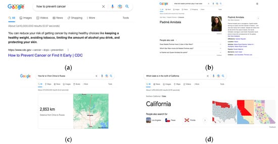
Figure 1.
Open-domain QA examples. The questions in (a,b) are about general knowledge, and (c,d) are about geographic domains. (a) Example of TextQA regarding general knowledge; (b) example of KBQA regarding general knowledge. (c,d) Simple questions that Google QA fails regarding geographic domains: (c) distance between adjacent countries (answer should be 0 or adjacent); (d) question about cardinal direction. This case study demonstrates that even Google QA fails at simple geographic questions that require simple geographic domain knowledge.
Although recent progress in NLP has significantly improved the performance of open-domain QA systems, there has been little research on open-domain QA systems specific to geographic questions. Even commercial QA products such as Google QA systems struggle to answer many simple geographic questions. Figure 1c,d show failure cases of Google QA systems adopted from [2]. Although these questions are easily answered by simple path traversals in geo-knowledge graphs (Geo-KG) if appropriate information exists, Google QA systems fail to answer these questions.
Researchers have studied the field of Geographic QA (GeoQA) to mitigate these problems. GeoQA can be segmented into Factoid GeoQA [2] and Geo-analytic QA [3,4], depending on the type of question. Factoid GeoQA answers questions based on geographic facts, whereas Geo-analytic QA focuses on questions with complex spatial analytical intents. In [5,6,7], the researchers focused on building rule-based GeoQA pipelines to solve questions in GeoQuestions201 [5], whereas geo-analytical questions using GeoAnQu were analyzed in [3,8].
Some research has been conducted on building the GeoQA dataset. In [5], a benchmark set of 201 geospatial questions were created from natural language questions and corresponding SPARQL/GeoSPARQL queries. However, these questions were developed by third-year undergraduate students without proper standards. The GeoAnQu dataset in [4] was generated from 100 scientific articles collected in the context of a master’s thesis at Utrecht University and textbooks on GIScience and GIS. GeoAnQu comprises 429 geo-analytic questions in the natural language without corresponding SPARQL/GeoSPARQL queries. The MS MARCO dataset [9] is a large-scale machine reading comprehension dataset. The dataset comprising diverse questions was generated from Bing’s search log sampling queries. Among the 1,010,916 questions, approximately 62,400 were location-relevant questions. Thus, [4,5] are small-scale datasets generated without proper standards, and [9] is a large-scale dataset generated from real-world queries.
However, there has been little research on the nature of questions in the geographic domain needed to build intelligent QA agents. Thus, the datasets in [4,5] contribute to building QA agents that fail to consider user interests and requirements.
Some studies have analyzed place-related questions that people ask and clustered similar questions on the basis of their own standard. A semantic encoding-based approach was proposed in [10] to investigate the structural patterns of real-world place-related questions on MS MARCO [9], which gathered data from real-world queries on search engines. In [4], a semantic encoding-based approach as in [10] was proposed to analyze the patterns in GeoQuestions201, GeoAnQu, and MS MARCO. Although [10] analyzed a large-scale GeoQA dataset that could represent real users’ interests and clustered similar questions, their methods were based on semantic encodings, which have limitations in representing similarities to those questions and therefore not commonly used techniques in topic modeling or Natural Language Processing (NLP). Furthermore, they did not present the latent topics of the clusters. Table 1 demonstrates the semantic encoding schema from [4], and Table 2 illustrates the results of applying semantic encoding schema to some questions in MS MARCO from [4]. As can be seen from Table 2, semantic encodings are not able to capture the words that are not detected as a predefined semantic encoding (e.g., the verb “located” is missing in the semantic encoding “1o”). Furthermore, it could not capture the semantics of the sentence because any arbitrary words that are classified using the same code (e.g., not only could “ores” be represented as “o”, but every word that is classified as an object will also be encoded as “o”) will be represented using the same code. That is, the semantic encoding-based approach could not fully capture the structure or semantic in a sentence, and could only roughly capture the structure of a sentence. Therefore, it could only roughly estimate the similarity of syntactic structure, and it could not assess the degree of semantic similarity. These problems will be addressed by adopting the embedding-based topic modeling approach.

Table 1.
Semantic representation encoding from [4]. Examples of each encoding are as follows: (1) place names (e.g., MIT); (2) place types (e.g., university); (3) activities (e.g., to study); (4) situations (e.g., to live); (5) qualitative spatial relationships (e.g., near); and (6) qualities (e.g., beautiful).
Table 2.
Examples of encoding patterns adopted from [4]. Natural language can be translated into semantic encodings. For example, “Where are ores located” could be translated into “1o” (where: 1; ores: o). This semantic encoding does not capture the verb “located”. This illustrates that the semantic encoding-based approach is not able to capture the structure of the whole sentence. Furthermore, the pattern “1o” will not be changed if “ores” are changed into any other arbitrary words. That is, it could not capture the semantics of the sentence. These problems will be addressed by adopting the embedding-based topic modeling approach.
Topic modeling is frequently used to discover latent semantic structures, referred to as topics, in a large collection of documents by clustering similar documents into a group. Latent Dirichlet allocation (LDA) and probabilistic latent semantic analysis are widely used topic-modeling techniques. Because these methods rely on the bag-of-words (BoW) representation of documents, which ignores the ordering and semantics of words, distributed representations of words and documents have recently gained popularity in topic modeling [11,12,13,14]. In particular, [11,12] proved that sentence embeddings in topic modeling produce more meaningful and coherent topics than topic models based on BoW or distributed word representations.
Therefore, we aim to group semantically similar questions into a cluster that has similar latent topics using an embedding-based topic modeling approach and utilize the topic modeling results to determine the users’ interest in the geographic domain. To the best of our knowledge, this is the first study to analyze geographic questions based on semantic similarity and determine the latent topics inside numerous geographic questions. The contributions of this study are as follows:
- We analyzed place-related questions based on semantic similarity. To the best of our knowledge, unlike existing works that have clustered structurally similar questions, this is the first study analyzing geographic questions based on semantic similarity.
- Because of the power of semantic similarity, we separated the geographic questions by clustering semantically similar questions.
- We demonstrated latent topics within an extensive collection of geographic questions. These results propose the direction of questions that GeoQA systems should handle to satisfy user needs.
Our paper is organized as follows. Section 2 describes previous works related to the GeoQA dataset and topic modeling. Then, in Section 3, we demonstrate the pipeline of topic modeling and provide a detailed description for each stage of topic modeling. In Section 4, we provide a description of the dataset to be analyzed, the setup of topic modeling, and how to evaluate the results of topic modeling. Section 5 provides the results in terms of a quantitative and qualitative evaluation. Section 6 presents a discussion of some of the results regarding model choices and their impact. Finally, in Section 7, we demonstrate the findings of our work, how these results could be utilized, the limitations of our study, and possible directions of future research.
2. Related Works
In this section, we discuss related work, starting with a brief overview of GeoQA (Section 2.1), the GeoQA dataset (Section 2.2), the analysis of GeoQA dataset (Section 2.3), and topic modeling (Section 2.4). Specifically, Section 2.1 and Section 2.2 provide an introduction to GeoQA and the GeoQA dataset. Section 2.3 demonstrates related research and our research in terms of analyzing geographic questions and finding latent topics inside them. Section 2.4 describes related studies with respect to topic modeling, which we used to analyze geographic questions and find latent topics within them.
Note that our research is primarily focused on analyzing the GeoQA dataset. Existing studies on analyzing the GeoQA dataset have utilized semantic encoding, which is not commonly used in the NLP field. The reason for this is that semantic encoding treats all words within a specific code as the same. That is, it may not distinguish different words with different meanings.
In order to represent documents, BoW representations have traditionally been used, and more recently, contextualized representations have been used. Both models are able to distinguish different words as different representations. However, BoW representations are not able to deliver contextual information, while contextualized representations are. Therefore, in terms of document representations, the semantic encoding-based approach has a severe limitation and thus is not widely used in NLP.
Therefore, it should be noted that although the contribution of our research is primarily in the area of GeoQA, the algorithms we used to improve upon existing GeoQA research came from the field of NLP. In other words, we used recently proposed algorithms in NLP to contribute to the field of GeoQA. Table 3 demonstrates the overview of related works.
Table 3.
Overview of related works. Our study contributes to the area of GeoQA, particularly in analyzing the GeoQA dataset by utilizing topic modeling methods with contextualized document embeddings recently proposed in the area of NLP.
2.1. Brief Overview of GeoQA
GeoQA is a sub-domain of QA that aims to answer geographic or place-related questions. GeoQA research can be divided into two categories: Factoid GeoQA and Geo-analytic QA.
Factoid GeoQA answers questions based on geographic facts. In [5], the authors implemented the first QA engine that could answer questions with a geospatial dimension. They proposed a template-based query translator that could translate a natural language following predefined templates into SPARQL/GeoSPARQL queries. Deep neural networks were used to improve the methods in [6,7] for named entity recognition, dependency parsing, constituency parsing, and BERT representations for contextualized word representations. Thus, they improved the accuracy of query generation results. However, that research also relied on a rule-based approach for translating natural language into SPARQL/GeoSPARQL queries. All these studies were conducted using GeoQuestions201, as discussed later.
Geo-analytic QA refers to answering geographic questions that require complicated geoprocessing workflows. Although some works [3,8] have studied Geo-analytic QA, no work has fully implemented the entire QA pipeline for Geo-analytic QA. In [3], the authors focused on why core concepts are essential for handling Geo-analytic QA, while in [8], language questions were translated into concept transformations. However, they failed to convert concept transformations into query languages such as SPARQL/GeoSPARQL. Although they translated natural language into intermediate structures, these can only be regarded as a partial implementation of Geo-analytic QA.
2.2. GeoQA Dataset
There are several datasets available for geographic questions. Nguyen et al. [9] introduced a large-scale machine-reading comprehension dataset named MS MARCO. The dataset comprises 1,010,916 anonymized questions sampled from Bing’s search query logs, each with a human-generated answer and 182,669 completely human-rewritten-generated answers. These datasets contained 6.17% location-related queries, i.e., approximately 62,000 queries. Although MS MARCO was originally introduced for real-world machine reading comprehension, to the best of our knowledge, it is the first and only large-scale geographic question corpus that has been studied.
GeoQuestions201 [5] comprises data sources, ontologies, natural language questions, and SPARQL/GeoSPARQL queries. These questions were answered by third-year students of the 2017–2018 Artificial Intelligence course in the authors’ departments. The students were asked to target three data sources (DBpedia, OpenStreetMap, and General Administrative Divisions dataset) by imagining scenarios in which geospatial information would be required and could provide intelligent assistance and propose questions with a geospatial dimension that they considered “simple”.
GeoAnQu [4] contains 429 geo-analytic questions compiled from scientific articles collected in the context of a master’s thesis at Utrecht University using Scopus and textbooks on GIScience and GIS. For scientific articles, the articles explicitly stated the questions in some cases, but in most cases, the authors manually formulated the question based on reading the article. For textbooks, they reformulated questions when they were not yet explicit.
GeoQuestions201 and GeoAnQu are small dataset made up of subjective, uncommon questions among public users, respectively. Therefore, there is no guarantee that the questions in [4,5] could represent a “natural” distribution of the information needs that users may want to satisfy using an intelligent assistant. As QA’s fundamental role is to answer users’ queries, a practical QA engine must be improved to satisfy the user’s request. In conclusion, the MS MARCO dataset would be a good fit for GeoQA tasks, as it comprises questions that were sourced from a real-world question-answering engine.
2.3. Analyzing the GeoQA Dataset
Several studies have analyzed GeoQA datasets. Hamzei et al. [10] analyzed MS MARCO in terms of its syntactic structure. Words or spans were encoded as semantic encodings such as place names, place types, activities, situations, qualitative spatial relationships, WH words, and other generic objects. They calculated the Jaro similarity [19] and applied the k-means clustering algorithm [20] to the encoded sentences. They also analyzed frequent patterns. However, because semantic encoding-based methods are based on syntactic structure, there is no guarantee of finding semantically similar clusters. Furthermore, they did not provide any latent topics of clusters.
In [4], MS MARCO, GeoQuestions201, and GeoAnQu were compared by adopting similar pipelines based on semantic encoding. They compared each dataset in terms of encoded patterns, such as n-gram patterns, encoded as predefined semantic encodings. They also analyzed and compared each dataset based on the frequency of specific words such as how, what, and when. However, because these works are based on word frequency or Jaro similarity in encoded patterns, there is no guarantee that these clusters share semantically similar topics. Furthermore, this work did not present any latent topic of the cluster.
2.4. Topic Modeling
The ability to organize, search, and summarize a large volume of text is a ubiquitous problem in NLP. Topic modeling is often used when a large collection of texts cannot be reasonably read and sorted by a person. Given a corpus comprising many texts, referred to as documents, a topic model will uncover latent semantic structures or topics in the documents. Topics can then be used to find high-level summaries of a large collection of documents, search for documents of interest, and group similar documents [13].
Conventional models, such as LDA [18] and non-negative matrix factorization (NMF) [21], describe a document as a bag of words, and model each document as a mixture of latent topics [11]. However, because BoW representations disregard the syntactic and semantic relationships among the words in a document, there are two main linguistic avenues to coherent text [12].
Recently, pre-trained language models have successfully been used to tackle a broad set of NLP tasks such as natural language inference, QA, and sentiment classification. Bianchi et al. [12] demonstrated that combining these contextualized representations, that is, BERT, with topic models produced more meaningful and coherent topics than traditional BoW topic models. Grootendorst [11] introduced BERTopic, which also uses pre-trained language models. It extends the clustering embedding approach described in [13,14] by incorporating a class-based variant of TF-IDF to create topic representations.
3. Topic Modeling Based on BERTopic
BERTopic generates topic representations in three steps: First, each document is converted into its embedding representation using a pre-trained language model. Then, the dimensionality of the resulting embeddings is reduced to optimize the clustering process and group similar embeddings into a cluster. Finally, topic representations are extracted from the document clusters using a custom class-based variation of TF-IDF [11].
We followed the BERTopic pipeline. However, BERTopic was applied on news articles, which are far different from questions in MS MARCO. Therefore, for each step, we included additional algorithms and a hyperparameter search to find appropriate settings for analyzing place-related questions in MS MARCO. Figure 2 shows the workflow of our approach and presents the difference between BERTopic and our approach.
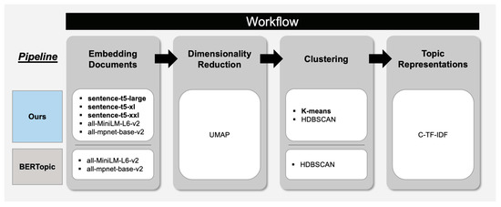
Figure 2.
Workflow of our approach. Our approach shares the same pipeline with BERTopic. However, our approach has more options for choosing the models.
Note that the word “document” refers to the question in MS MARCO. We will interchangeably use the word “document” and “question”, depending on the context. However, “document” and “question” are the same in our experiments.
3.1. Sentence Embeddings
In BERTopic, the authors assumed that documents containing the same topic were semantically similar. BERTopic used the Sentence-BERT (SBERT) [16] framework to perform the embedding step. As a baseline model [11], all-MiniLM-L6-v2 (MiniLM) and all-mpnet-base-v2 (MP-NET) SBERT models were used.
As mentioned in [11], any other embedding can be used if the language model is fine-tuned for semantic similarity; thus, the quality of clustering in BERTopic is enhanced as new and improved language models are developed. We explored better sentence embedding models when applying BERTopic to place-related questions.
Sentence-T5 (ST5) [17] first explored sentence embeddings from text-to-text transformers (T5) [22] and demonstrated that with proper fine-tuning strategies, ST5 outperformed SBERT/SRoBERTa and SimCSE [23] in SentEval and SentGLUE transfer tasks, including semantic textual similarity.
Therefore, in addition to all-MiniLM-L6-v2 (MiniLM) and all-mpnet-base-v2 (MP-NET) SBERT models, which are baselines for BERTopic, we further utilized the sentence-t5-large, sentence-t5-xl, and sentence-t5-xxl ST5 models. In addition to sentence-t5-large, we used the sentence embeddings of ST5 Enc 3B and 11B because [17] demonstrated that scaling up the model size greatly improves sentence embedding quality. In conclusion, we used sentence-t5-large, sentence-t5-xl, and sentence-t5-xxl in addition to BERTopic’s baseline MiniLM, MP-NET.
3.2. Clustering
In BERTopic, before clustering similar documents based on sentence embeddings, the dimension of embeddings is reduced. To reduce the dimensionality of document embeddings, instead of traditional PCA [24] or t-SNE [25], they used UMAP [26], which has been shown to preserve more local and global features of high-dimensional data in lower projected dimensions [26].
To cluster the reduced embeddings, they used HDBSCAN [27] models, which uses a soft-clustering approach, allowing noise to be modeled as outliers. This prevents unrelated documents from being assigned to any cluster and is expected to improve the topic representation. Moreover, [28] demonstrated that reducing high-dimensional embeddings with UMAP can improve the performance of well-known clustering algorithms, such as k-means and HDBSCAN, in terms of clustering accuracy and time.
Note that our purpose is to identify the users’ interest in the geographic domain; it could be problematic if too many documents are classified as outliers, since outliers could be regarded as a single cluster. To prevent the generation of outliers, in addition to the baseline of BERTopic (HDBSCAN), we include k-means as the clustering method, which is popular among hard-clustering approaches.
3.3. Topic Representation
For topic representation, we followed the method used in [11]. After clustering, we represent each topic using class-based TF-IDFs, which are variants of the classical TF-IDF proposed in [11]. The classic TF-IDF represents the importance of a word in a document as follows:
where is the weight of term t in document d, is the number of documents in the collection, is the frequency of term t in document d, and is the frequency of term t in the collection. Under certain assumptions, summing up TF-IDF for all possible words and documents could be interpreted as mutual information between the probability distribution over documents and probability distribution over terms [29].
To generalize TF-IDF from a document to a cluster of documents, [11] treats all documents in a cluster as a single document by concatenating the documents. Subsequently, TF-IDF is adjusted to account for this representation by translating documents into clusters [11]. These could generate representations of topics that we call class-based TF-IDF, in short, c-TF-IDF. To reduce the number of topics into specified values, [11] merged each cluster by iteratively merging the c-TF-IDF representations of the least common topic with its most similar one. The equations for the c-TF-IDF are as follows:
where is a collection of documents concatenated into a single document for each cluster, refers to the term frequency of term t in class c, A is the average number of words per class, and is the frequency of term t across all classes. To output only positive values, 1 is added to the division within the logarithm [11].
4. Experimental Setup
4.1. Dataset
MS MARCO was introduced in [9] to handle the problems of the existing dataset. Existing datasets are not sufficiently large to train deep neural networks, or even if there are large-scale machine-reading comprehension datasets, they are often synthetic. Furthermore, a common characteristic shared by many of these datasets is that the questions are generally generated by crowd workers based on the provided text spans or documents. In contrast, in MS MARCO, the questions correspond to actual search queries that users have submitted to Bing, and therefore may be more representative of a “natural” distribution of the information needs that users may want to satisfy using, say, an intelligent assistant [9]. For this reason, we selected MS MARCO as our geographic question dataset.
Table 4 shows the distribution of questions based on an answer-type question classifier and the proportion of questions that explicitly contain words like “what” and “where”, adopted from [10]. Nearly 6.17% of the questions were related to location. For our experiments, we only used location-type questions in the training set. We retrieved 50,893 questions from the training set and performed exploratory data analysis.
Table 4.
Distribution of questions based on the answer-type question classifier and the proportion of the questions that exactly contain the specific word in MS MARCO. This table is adopted from [9].
We analyzed the same question containments as in [9]. In Table 5, 55.63% of our questions contain “where”, and 34.35% of our questions contain “what”. In Table 4, although only 3.46% of the original MS MARCO contains the “where” segment, 55.63% of location-related questions contain the “where” segment.
Table 5.
The proportion of the questions that exactly contain the specific word in location-related questions in MS MARCO.
We also analyzed the length of the questions. Figure 3 shows a histogram of question length, and Table 6 shows the statistics of question length. Most of the length lies between 4 and 8 words, and the average question length is 6.08 words. We retained questions shorter than 20 words, resulting in 50,859 questions.
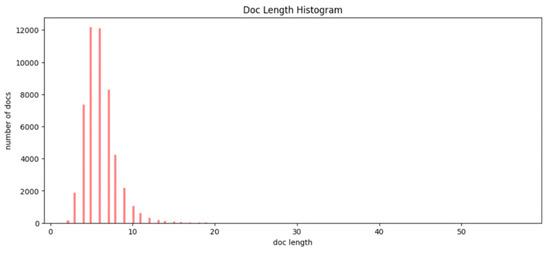
Figure 3.
Histogram of document lengths. The X-axis represents the question (document) length, which is the number of words in each question. The Y-axis represents the number of questions with the specific value of question length. Most of the questions have a length between 4 and 8 words.
Table 6.
Statistics of question length. The question length refers to the number of words in each question. The maximum question length is 57 words, and the minimum question length is 2 words. The average length of questions is 6.08 words.
4.2. Models
We adopted the same pipeline as BERTopic to analyze the questions. Because most of our questions contain less than 10 words, the default hyperparameters used by BERTopic [11] could be inappropriate. Therefore, we conducted experiments to tune hyperparameters for BERTopic before analyzing the questions. Specifically, we tested variations in sentence embedding models, target dimensions for UMAP dimensionality reduction, and clustering methods. The experimental setup is presented in Table 7.
Table 7.
Experimental setup for BERTopic.
For sentence embeddings, we used the base model, all-MiniLM-L6-v2, and all-mpnet-base-v2, as in [11]. Because these models are tuned for all-round models for many use-cases, we additionally tested models that had been specifically fine-tuned for sentence-similarity tasks, sentence-t5-xxl, sentence-t5-xl, and sentence-t5-large, depending on their model sizes. A detailed description of the embedding models is provided in Table 8.
Table 8.
Detailed description of the sentence embedding models.
For the clustering method, we used HDBSCAN, which is the base model in [11]. Because HDBSCAN is a soft-clustering algorithm that can produce outliers, we also added k-means, which is a widely used hard-clustering algorithm. If there were too many outliers, analyzing the results of the topic model would be difficult. Because HDBSCAN is robust to parameter selection [24], we did not tune any of the parameters in HDBSCAN.
4.3. Evaluation
We evaluated the topic model quantitatively and qualitatively. In terms of quantitative measures, we adopted a widely used metric for assessing the quality of topic model, topic coherence [11,12,13,14], and for qualitative measures, we manually inspected the randomly sampled questions inside each cluster.
In terms of quantitative evaluation, for each topic, we evaluated topic coherence using normalized pointwise mutual information [30]. This coherence measure has been shown to emulate human judgment with reasonable performance [31]. The topic coherence ranges from (−1, 1), where 1 indicates a perfect association. The idea behind topic coherence is that a coherent topic will display words that tend to occur in the same documents. In other words, the most likely words in a coherent topic should have high mutual information. Document models with higher topic coherence are more interpretable topic models [32]. The equation for the normalized pointwise mutual information is as follows:
where w is the list of top-N words for a topic. For a model generating K topics, the overall NPMI score is an average across all topics. We set as NPMI and N as 20.
In terms of qualitative evaluation, we evaluated the quality of results in two regards: topic representativeness and geographic relatedness. In order to assess both aspects, we randomly sampled 10 questions in each topic and manually labeled whether the question satisfied the criteria (we only sampled 10 questions to ease the burden of manual annotation, and they were labeled by two of the authors). Specifically, we investigated whether the top 10 words in terms of c-TF-IDF value well represented the question inside each cluster (i.e., we labeled c-TF-IDF words if the words could be considered a latent topic for specific documents). Furthermore, for each cluster, we evaluated the percentage of geographic questions (i.e., we labeled the question as a geographic question; if it is either a factoid geographic question or a geo-analytic question in [2]). To analyze geographic questions and identify the users’ interest lying within the questions, we assumed that geographic questions should be separated first from non-geographic ones. Furthermore, because topics can be used to find high-level summaries of a large collection of documents, search for documents of interest, and group similar documents, it would be crucial to obtain topics that are relevant to the documents in each cluster.
In conclusion, it would be useful if topic models could (1) classify semantically similar questions into a single cluster (topic coherence), (2) output topic representations that give high-level summaries inside each cluster (topic representativeness), and (3) well separate the geographic questions from non-geographic ones (geographic relatedness).
5. Results
5.1. Model Selection for BERTopic
We conducted experiments to systematically determine the hyperparameters for the BERTopic pipelines. As shown in Table 7, we conducted various experiments on variants of embedding models, different target embedding dimensions by UMAP, and clustering methods. All experimental results are presented in Table A1. We evaluated the performance of topic models using topic coherence, topic representativeness, and geographic relatedness.
5.1.1. Sentence Embedding Model Selection
First, we demonstrate our results using sentence-embedding models. Table 9 summarizes the results. Ranging from 5 to 15, UMAP dimensions in steps of 5 (three runs for UMAP configurations) and two clustering methods (two runs for cluster configurations) results in six configurations. All results were averaged across three runs for each configuration. Therefore, each case in Table 9 was an average of topic coherence score for 18 separate runs (3 types of UMAP dimension configuration × 2 clustering methods × 3 runs for each step). We bolded the top nine (30%) scores for the 30 cases (ranging from topic size 50 to 200 with step size 30. For each number of topics, there are five sentence embedding models. Thus, 5 sentence embedding models × 6 configurations of number of topics = 30 cases). Sentence-t5-xxl has three cases left over. Furthermore, sentence-t5-xxl has the top performance among the 30 cases. We can think of this as a bigger model that is able to model sentence similarity better than smaller models. Therefore, we selected sentence-t5-xxl as our embedding model and the number of topics as 50, as these conditions showed the best performance among the 30 cases.
Table 9.
Experimental results on sentence embeddings. Ranging from topic size 50 to 200 with step size 30. For each number of topics, we have 5 sentence embedding models. Thus, 5 sentence embedding models × 6 configurations of number of topics results in 30 cases. For each case (entry in the table), we averaged the score of 18 separate runs (3 types of run for the UMAP dimension, 2 types of clustering method, and 3 runs for each configuration). Therefore, each entry represents the topic coherence value averaged on 18 runs. Sentence-t5-xxl with number of topics 50 shows the best topic coherence.
5.1.2. Clustering Model Selection
Table 10 presents the detailed results for sentence-t5-xxl with 50 topics. In all cases, k-means clustering showed better performance than HDBSCAN. Furthermore, over 50% of the documents were classified as outliers when applying HDBSCAN. We selected the final model that showed the highest coherence score. That is, we chose the UMAP target dimension as 15 and clustering methods as k-means.
Table 10.
Experimental results of clustering model selection. All the results were obtained with sentence-t5-xxl as the sentence embedding model and 50 as the number of topics.
In conclusion, our final model uses sentence-t5-xxl as an embedding model, 50 for the number of topics, 15 for the UMAP dimension, and k-means for clustering methods.
5.1.3. Results of Clustering Sentence Embeddings
In this section, we present the results of topic modeling. Topic modeling groups semantically similar documents into clusters. Figure 4a shows the results of topic modeling. We segmented 50,859 documents into 50 topics and labeled them in descending order of the number of documents. Figure 4b shows a histogram of the number of documents per topic. The number of documents per topic was distributed in a bell-shaped manner. Because the distribution is not skewed, our documents are not assigned to a few topics, but rather to diverse topics.
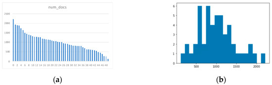
Figure 4.
Results of topic modeling: (a) distribution over number of documents per topic; (b) histogram of number of documents per topic. As can be seen from (a), we named each topic in descending order of number of documents. That is, topic 0 has the highest number of documents. Detailed description of each topic is provided in Table A2.
5.2. Analyzing Location-Relevant Questions in MS MARCO
In Section 5.1, we evaluated the quality of topic models in terms of topic coherence. This section analyzes the representativeness of topic representation, geographic relatedness of questions in MS MARCO, and users’ interest implicit in the large collection of questions.
5.2.1. Analyzing High-Level Summaries in a Large Collection of Questions
Topic modeling can provide high-level summaries in a large collection of documents using topic representation. Therefore, we examined whether our topic representations provided high-level summaries for each topic following the methods mentioned in Section 4.3.
Table 11 shows the top 10 words in terms of c-TF-IDF scores, and examples labeled with the top 10 words for topic 4. Topic 4 could be represented as the top 10 words with the highest c-TF-IDF values. For example, the most representative word in topic 4 is “ca” (which stands for California). Next, we can see “California” as the top 2 representative words. Other words, such as “county” and “san” follow. For the 0th document (the index will start from 0, not 1), “what county is the city of la Puente, ca”, we labeled it as 0, 1, because the terms “ca” and “california” well represent the underlying topic. Following the mentioned labeling criteria, we manually labeled 10 questions per topic, the results of which are shown in Figure 5.
Table 11.
Manual annotation example for topic 4 regarding c-TF-IDF representativeness. We labeled each document (column Documents) with the index of relevant c-TF-IDF words (column c-TF-IDF index). Column c-TF-IDF info does not have any relation with documents column. For simplicity, we only put them together with the documents. That is, the 0th element in c-TF-IDF info is independent from the 0th element in Documents.
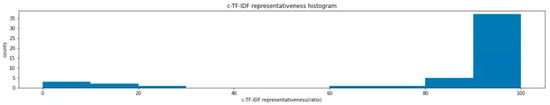
Figure 5.
Histogram of c-TF-IDF representativeness ratio. The X-axis represents the c-TF-IDF representativeness as a ratio, and the y-axis represents how many topics have specific values of c-TF-IDF representativeness. For example, if c-TF-IDF representativeness is 90%, it means that approximately 90% of questions in a cluster could be explained by words with top 10 c-TF-IDF value.
It should be noted that the word “california” and “ca” are in the topic representations for same topic. We could see the other region name and its abbreviation grouped into a single cluster in Table A2 as well. We did not do any processing for the word “ca” or “california.” However, contextualized embeddings have the ability to identify semantic information (i.e., words with similar meaning will occur in similar context). Therefore, a sentence with words “ca” and “california” are grouped into a single cluster.
Figure 5 shows the results of the manual annotation represented by the histogram. Most of the questions in each topic can be represented by c-TF-IDF. If we count the number of topics that exceeds 80% in the c-TF-IDF representativeness ratio, we obtain 42 out of 50 topics. Therefore, we could obtain high-level summaries in a large collection of questions using topic representations and c-TF-IDF scores. Because eight topics have less than 80% in the c-TF-IDF representativeness ratio, and most of them are in the range of 0–30%, there is room for improvement in terms of the representativeness of c-TF-IDF topic representation.
Table 12 shows the documents in the examples of topics and the corresponding sampled documents with 100% representativeness. In topic 2, “where” well represents the high-level summaries of the document collection. In topic 3, “body” demonstrates the high-level summaries of those clusters. That is, high-level summaries are obtained from the topic representations. Furthermore, by interpreting topic representations, we doubt whether topic 3 is really related to geographic topics. These findings guide us to the next section, which analyzes the geographic relatedness of topics.
Table 12.
Manual annotation example for topics 2, 3 regarding c-TF-IDF representativeness. All the documents in topic 2 could be well represented by the 0th topic word “where”, and all the documents in topic 3 could be well represented by the word “body.” For example, the 1st and 2nd documents in topic 2, “where is salalah” and “where is balkin”, could be explained by the word “where”. For topic 3, “where are the vocal cords in the body” and “where is testosterone produced in males” could be well represented by the word “body”. By inspecting the topic words in topic 2 (e.g., where located, location, india, province) and topic 3 (body, located, blood, pain, brain), we can speculate that topic 2 is related to geographic location and topic 3 is related to location with respect to our body.
5.2.2. Analyzing Geographic Relatedness of the Questions
Although we only used location-relevant questions in MS MARCO, there could have been questions that were not related to location. The reason for this is that the classification in Table 4 was performed automatically by a machine learning-based classifier, resulting in some prediction error. Furthermore, some questions could be relevant to locations, but not geographically.
Therefore, we investigated whether these questions were related to the geographic domain. We labeled the geographic relatedness of the sampled documents in Section 5.2.1. Table 13 shows examples of manual labeling. For example, the question “where is paloma” is a geographic question, but “where are the vocal cords in the body” is not.
Table 13.
Manual annotation examples for topic 2 regarding geographic relatedness. For each document, we manually annotated that the documents are related to the geographic domain or not. For example, “where is the karate seika tandem located” is a geographic question, because it is a factoid geographic question in [2] that asks the location of a geographic entity. However, “where is the paper behind the bar” could be considered to be visual question answering. The 9th document, “where is harvey weinstein in january”, asks a specific person’s location at a specific moment. We labeled it as a non-geographic question because it is neither a factoid geographic question nor a geo-analytic question as defined in [2].
Figure 6 shows the results of the manual annotations and shows the ratio of geographic questions per topic. A total of 36 out of 50 clusters exceeded 80% in the ratio of geographic questions. However, for 8 out of 50 clusters, less than 20% were geographic questions. Most of the topics were distributed near either 100% or 0%. In other words, our topic model separated the topics with geographic questions from those with nongeographic questions.
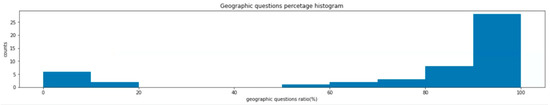
Figure 6.
Histogram of geographic question ratio. The X-axis represents the geographic questions ratio ranging from 0% to 100% (by step size of 10%). The Y-axis represents the number of topics (counts) with specific geographic questions ratio. Over 25 topics possess 100% geographic relatedness.
Table 14 presents examples of geographic and non-geographic topics. Topic 3 contains questions about location, but not geographic location, because there are topic words like “body”, “blood”, and “pain”. In topic 4, most of the questions were relevant to geographic locations in California. Furthermore, topic 4 may be a geographic topic, because it contains words like “CA”, “California”, and “county”. Therefore, using topic representations, we could filter out geographic topics from non-geographic ones.
Table 14.
Manual annotation example for topics 3, 4 regarding c-TF-IDF representativeness and geographic relatedness.
5.2.3. Analyzing Geographic Questions
This section analyzes geographic questions based on the results in Section 5.2.1 and Section 5.2.2. Table 15 summarizes the results in Section 5.2.1 and Section 5.2.2. The top 10 words for each topic are all in Table A2. Geographic topics refer to a topic in which more than 80% of questions are related to the geographic domain (as in Section 5.2.2), and representative topics refer to topics in which more than 80% of questions could be represented by topic words (as in Section 5.2.1). We found that 36 out of 50 were topics that were geographic and representative. These clusters were further analyzed.
Table 15.
Topic segmentation based on results in Section 5.2.1 and Section 5.2.2.
Figure 7 visualizes a hierarchical structure of topics using Ward’s linkage function to perform the hierarchical clustering based on the cosine distance matrix between topic embeddings. This clustering is for visualization purposes; therefore, topics that are not related could be clustered. The clusters with topics 46, 48, 47, 42, 49 show that people are curious about zip or area codes (46) and time zones (42). The clusters with topics 13, 27 are inquiries about where to find something or where some creature lives (13). In addition, we were able to figure out locations where something is made or can be bought (27). The cluster with topics 1, 21 is related to locations where a movie is filmed (21) and where someone was born or buried. In addition, people are curious about the county information regarding specific regions such as California and Michigan. We found a pattern whereby people frequently use the abbreviation of the state’s name, such as “CA” for “California” and “MI” for “Michigan”. As noted earlier, because of the power of contextualized document embeddings, we were able to successfully group sentences with region name and its abbreviation (“California” and “CA”, “Michigan” and “MI”, and so on).
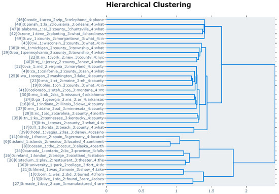
Figure 7.
Latent topics of geographic questions in MS MARCO. Hierarchical clustering in this figure is only for visualization purposes. We discovered the users’ interest regarding geographic domains by investigating the latent topics. For example, people are interested in time zones (topic 42), zip or area codes (topic 47), and where something is made or can be bought (topic 27).
Thus, we successfully identified latent topics by inspecting geographic topics with representative topic representations. That is, we were able to determine the users’ interests and requirements regarding GeoQA. These would be important findings as they could guide the current GeoQA systems in aspects requiring improvement.
6. Discussion
In this section, we provide a discussion regarding our choice of models and their impact on our results. Specifically, we discuss sentence embedding, clustering, and c-TF-IDF representations.
Our results show that Sentence T5 consistently outperformed SBERT in terms of topic coherence. The reason for this is the quality of sentence embedding, as it was previously shown in [17] that Sentence T5 consistently outperformed SBERT in various downstream tasks. Furthermore, the best performing model was the biggest model (i.e., sentence-t5-xxl). This result is also coherent with existing studies reporting that models with larger size with appropriate fine-tuning consistently outperform smaller ones (sentence-t5-large vs. sentence-t5-xl).
For clustering algorithms, k-means clustering consistently outperformed HDBSCAN. This was coherent with existing studies [28] reporting that for a dataset with more than 2k samples, k-means clustering consistently outperforms HDBSCAN. Before applying clustering algorithms, we adopted dimensionality reduction, UMAP. As clustering algorithms tend to suffer from the curse of dimensionality [28] (i.e., high-dimensional data (in our case 384 for all-MiniLM-L6-v2 and 768 for other models) often require an exponentially growing number of observed samples to obtain a reliable result), this is essential to improve the clustering accuracy and time. As can be seen from Table A2, the choice of UMAP embedding dimension (among 5, 10, 15) has little impact on the performance.
Our results demonstrate that c-TF-IDF representations well represent the topics. However, we did not remove the stop words while building the topic representations. With proper postprocessing, such as stop word removal, we could enhance the quality of topic representations. Furthermore, we did not study the relationships between each topic. That is, if we had investigated the topic representations in terms of topic similarity with pairs of clusters, we could have obtained more comprehensive high-level summaries in a large collection of geographic questions. We leave this to future work.
7. Conclusions
This study analyzed geographic questions based on their semantic similarity and identified the geographic topics of interest. Existing studies have analyzed geographic questions in terms of syntactic structures, which have limitations in terms of representing semantic information and do not identify latent topics. To the best of our knowledge, this is the first study to analyze geographic questions in terms of semantic similarity and demonstrate the corresponding latent topics.
The BERTopic pipeline was adopted to cluster similar questions and discover latent topics. Following the BERTopic pipeline, we performed various experiments with different hyperparameters to select the appropriate models. Thus, we successfully selected topic models with high topic coherence to find the semantic structure of numerous documents.
A manual inspection showed the effectiveness of the embedding-based topic modeling approach and discovered the latent geographic topics that are of interest. First, we determined that topic representations generated by embedding-based topic modeling offer high-level summaries of numerous documents. Second, because of the coherent collection of documents inside each cluster and high-level summaries provided by topic representation, we effectively separated geographic and non-geographic clusters. Third, by inspecting geographic questions with higher topic representativeness, we demonstrated latent topics within several geographic questions. These findings show geographic topics that people of interest therefore propose regarding the direction of questions that GeoQA systems should handle to satisfy user needs.
Although this research proposes a direction that GeoQA systems would follow, there is a limitation in that we analyzed the MS MARCO dataset. Although MS MARCO gathered questions from real users’ queries, this dataset was generated a few years ago and is outdated. Furthermore, all queries from MS MARCO were collected from Bing and could be biased in terms of user distribution, such as nationality. Therefore, future studies should analyze recent questions asked by users of a representative search engine.
Author Contributions
Conceptualization, Jonghyeon Yang and Hanme Jang; methodology, Jonghyeon Yang and Hanme Jang; software, Jonghyeon Yang; validation, Jonghyeon Yang; formal analysis, Jonghyeon Yang and Hanme Jang; investigation, Jonghyeon Yang and Hanme Jang; resources, Kiyun Yu; data curation, Jonghyeon Yang; writing—original draft preparation, Jonghyeon Yang; writing—review and editing, Jonghyeon Yang and Hanme Jang; visualization, Jonghyeon Yang and Hanme Jang; supervision, Kiyun Yu; project administration, Kiyun Yu; funding acquisition, Kiyun Yu. All authors have read and agreed to the published version of the manuscript.
Funding
This work was supported by the Korea Agency for Infrastructure Technology Advancement (KAIA) grant funded by the Ministry of Land, Infrastructure and Transport (Grant RS-2022-00143336).
Data Availability Statement
Not applicable.
Conflicts of Interest
The authors declare no conflict of interest.
Appendix A
Table A1.
Experimental results.
Table A1.
Experimental results.
| Number of Topics | UMAP Target Dimension | Clustering Method | Sentence-t5-Large | Sentence-t5-xl | Sentence-t5-xxl | All-MiniLM-L6-v2 | All-Mpnet-Base-v2 |
|---|---|---|---|---|---|---|---|
| 200 | 5 | k-means | −0.1330056 | −0.1345761 | −0.1277029 | −0.1848673 | −0.141093 |
| HDBSCAN | −0.1433254 | −0.1457019 | −0.1346459 | −0.1899744 | −0.1390007 | ||
| 10 | k-means | −0.1328044 | −0.1358003 | −0.1305998 | −0.1800947 | −0.1396308 | |
| HDBSCAN | −0.149201 | −0.148722 | −0.1338223 | −0.1908829 | −0.1452692 | ||
| 15 | k-means | −0.1283197 | −0.1351717 | −0.1301532 | −0.1792993 | −0.1375294 | |
| HDBSCAN | −0.1518844 | −0.1475704 | −0.1325517 | −0.1931541 | −0.1445527 | ||
| 170 | 5 | k-means | −0.1221535 | −0.1264646 | −0.1216601 | −0.1841559 | −0.1344245 |
| HDBSCAN | −0.1390226 | −0.1412985 | −0.132338 | −0.1895984 | −0.1388525 | ||
| 10 | k-means | −0.1217009 | −0.1269646 | −0.124053 | −0.1792774 | −0.1361282 | |
| HDBSCAN | −0.1481609 | −0.1462774 | −0.1295757 | −0.1936876 | −0.1430434 | ||
| 15 | k-means | −0.1207681 | −0.1281991 | −0.1241469 | −0.1777497 | −0.1319709 | |
| HDBSCAN | −0.1520077 | −0.1453113 | −0.1272713 | −0.1942368 | −0.1453793 | ||
| 140 | 5 | k-means | −0.1111789 | −0.12412 | −0.105158 | −0.1754365 | −0.1221885 |
| HDBSCAN | −0.1317304 | −0.1395091 | −0.1243175 | −0.1905828 | −0.136829 | ||
| 10 | k-means | −0.104936 | −0.1124119 | −0.1093309 | −0.1714171 | −0.1231637 | |
| HDBSCAN | −0.142058 | −0.1415791 | −0.1254096 | −0.1956751 | −0.1415105 | ||
| 15 | k-means | −0.1061068 | −0.1156702 | −0.1107736 | −0.1715579 | −0.1247703 | |
| HDBSCAN | −0.1435889 | −0.1441576 | −0.1283509 | −0.1974347 | −0.1421 | ||
| 110 | 5 | k-means | −0.0800038 | −0.1030744 | −0.0867998 | −0.1577837 | −0.1051492 |
| HDBSCAN | −0.1210283 | −0.1262859 | −0.1139022 | −0.1823657 | −0.1216611 | ||
| 10 | k-means | −0.0843599 | −0.0969733 | −0.0892971 | −0.1597336 | −0.1040341 | |
| HDBSCAN | −0.1327209 | −0.1293402 | −0.1138686 | −0.1905848 | −0.1320657 | ||
| 15 | k-means | −0.0808714 | −0.0945484 | −0.0900181 | −0.158812 | −0.1012225 | |
| HDBSCAN | −0.1331814 | −0.1317335 | −0.1166595 | −0.1947135 | −0.1333675 | ||
| 80 | 5 | k-means | −0.0504757 | −0.069031 | −0.0505063 | −0.1174056 | −0.0673501 |
| HDBSCAN | −0.0838284 | −0.1015199 | −0.0846814 | −0.1693818 | −0.1017107 | ||
| 10 | k-means | −0.0524889 | −0.0695422 | −0.0538084 | −0.1131622 | −0.0668695 | |
| HDBSCAN | −0.1008166 | −0.1001257 | −0.0837272 | −0.1868712 | −0.120024 | ||
| 15 | k-means | −0.0513399 | −0.0606748 | −0.047895 | −0.1148984 | −0.0653315 | |
| HDBSCAN | −0.113378 | −0.1067271 | −0.0866257 | −0.1893554 | −0.112851 | ||
| 50 | 5 | k-means | −0.0192551 | −0.0414722 | −0.0185964 | −0.0460959 | −0.0261569 |
| HDBSCAN | −0.0494421 | −0.0649573 | −0.0444795 | −0.130683 | −0.0750043 | ||
| 10 | k-means | −0.0173773 | −0.0305339 | −0.0186774 | −0.0456125 | −0.0312847 | |
| HDBSCAN | −0.0657178 | −0.0594805 | −0.0424092 | −0.1537143 | −0.0828262 | ||
| 15 | k-means | −0.0196226 | −0.0298843 | −0.0182411 | −0.0434182 | −0.0251376 | |
| HDBSCAN | −0.0636553 | −0.0641457 | −0.0439653 | −0.1626524 | −0.0823663 |
Table A2.
Topic information. Each row represents the top 10 words in each topic.
Table A2.
Topic information. Each row represents the top 10 words in each topic.
| 0 | 1 | 2 | 3 | 4 | 5 | 6 | 7 | 8 | 9 | |
|---|---|---|---|---|---|---|---|---|---|---|
| 0 | (‘island’, 0.0561) | (‘islands’, 0.0393) | (‘mexico’, 0.0348) | (‘located’, 0.0262) | (‘continent’, 0.0242) | (‘of’, 0.023) | (‘hawaii’, 0.023) | (‘the’, 0.0219) | (‘is’, 0.0211) | (‘china’, 0.0203) |
| 1 | (‘born’, 0.1375) | (‘was’, 0.0964) | (‘did’, 0.05) | (‘buried’, 0.0475) | (‘from’, 0.0468) | (‘live’, 0.0378) | (‘where’, 0.0305) | (‘up’, 0.0277) | (‘die’, 0.0242) | (‘grow’, 0.022) |
| 2 | (‘where’, 0.0385) | (‘is’, 0.0321) | (‘located’, 0.0215) | (‘location’, 0.015) | (‘now’, 0.0149) | (‘india’, 0.0139) | (‘the’, 0.013) | (‘province’, 0.0113) | (‘of’, 0.0089) | (‘at’, 0.0086) |
| 3 | (‘your’, 0.0526) | (‘body’, 0.0432) | (‘the’, 0.0394) | (‘located’, 0.0379) | (‘are’, 0.0325) | (‘does’, 0.0285) | (‘where’, 0.0268) | (‘blood’, 0.026) | (‘pain’, 0.0237) | (‘brain’, 0.0211) |
| 4 | (‘ca’, 0.1687) | (‘california’, 0.0905) | (‘county’, 0.0397) | (‘san’, 0.0347) | (‘what’, 0.0289) | (‘is’, 0.0265) | (‘in’, 0.024) | (‘beach’, 0.0223) | (‘valley’, 0.0193) | (‘santa’, 0.0182) |
| 5 | (‘did’, 0.0384) | (‘of’, 0.0335) | (‘the’, 0.0313) | (‘was’, 0.027) | (‘war’, 0.0248) | (‘battle’, 0.023) | (‘continent’, 0.0228) | (‘greece’, 0.0209) | (‘were’, 0.0198) | (‘located’, 0.0194) |
| 6 | (‘most’, 0.0931) | (‘largest’, 0.0861) | (‘world’, 0.0701) | (‘biggest’, 0.0547) | (‘cities’, 0.0487) | (‘highest’, 0.0435) | (‘us’, 0.0408) | (‘places’, 0.0379) | (‘the’, 0.0364) | (‘longest’, 0.0353) |
| 7 | (‘headquarters’, 0.0913) | (‘address’, 0.0858) | (‘hospital’, 0.0575) | (‘located’, 0.034) | (‘mailing’, 0.0331) | (‘bank’, 0.0269) | (‘where’, 0.0236) | (‘based’, 0.0208) | (‘center’, 0.0184) | (‘store’, 0.018) |
| 8 | (‘ocean’, 0.0415) | (‘the’, 0.0376) | (‘occur’, 0.0304) | (‘alaska’, 0.0298) | (‘earth’, 0.0289) | (‘are’, 0.0267) | (‘river’, 0.0262) | (‘desert’, 0.0245) | (‘of’, 0.02) | (‘most’, 0.0195) |
| 9 | (‘tx’, 0.1802) | (‘texas’, 0.1748) | (‘county’, 0.0446) | (‘what’, 0.0314) | (‘is’, 0.0272) | (‘in’, 0.0256) | (‘dallas’, 0.0217) | (‘houston’, 0.0173) | (‘located’, 0.0157) | (‘san’, 0.0152) |
| 10 | (‘from’, 0.1179) | (‘come’, 0.1163) | (‘name’, 0.1068) | (‘originate’, 0.0907) | (‘did’, 0.0901) | (‘does’, 0.0682) | (‘word’, 0.0421) | (‘the’, 0.0402) | (‘term’, 0.0385) | (‘last’, 0.0377) |
| 11 | (‘from’, 0.0725) | (‘come’, 0.0705) | (‘grow’, 0.0659) | (‘originate’, 0.0533) | (‘does’, 0.0522) | (‘did’, 0.0393) | (‘grown’, 0.039) | (‘do’, 0.0342) | (‘where’, 0.0306) | (‘trees’, 0.03) |
| 12 | (‘airport’, 0.2397) | (‘closest’, 0.0734) | (‘to’, 0.061) | (‘terminal’, 0.0467) | (‘fly’, 0.0426) | (‘airlines’, 0.0314) | (‘international’, 0.0301) | (‘airports’, 0.028) | (‘near’, 0.0257) | (‘what’, 0.0253) |
| 13 | (‘live’, 0.1405) | (‘do’, 0.1038) | (‘found’, 0.0493) | (‘are’, 0.0406) | (‘does’, 0.0332) | (‘where’, 0.031) | (‘from’, 0.0242) | (‘habitat’, 0.0216) | (‘come’, 0.0195) | (‘wild’, 0.0182) |
| 14 | (‘italy’, 0.0628) | (‘france’, 0.0473) | (‘spain’, 0.044) | (‘germany’, 0.0421) | (‘located’, 0.0253) | (‘where’, 0.0242) | (‘is’, 0.0242) | (‘of’, 0.0216) | (‘the’, 0.0207) | (‘region’, 0.018) |
| 15 | (‘states’, 0.1261) | (‘state’, 0.0741) | (‘which’, 0.0534) | (‘has’, 0.0414) | (‘have’, 0.0406) | (‘marijuana’, 0.0313) | (‘most’, 0.0307) | (‘prison’, 0.0284) | (‘the’, 0.0282) | (‘us’, 0.0271) |
| 16 | (‘il’, 0.1694) | (‘indiana’, 0.1108) | (‘illinois’, 0.087) | (‘iowa’, 0.0869) | (‘county’, 0.0526) | (‘ia’, 0.039) | (‘what’, 0.0374) | (‘in’, 0.0327) | (‘is’, 0.0278) | (‘township’, 0.0151) |
| 17 | (‘fl’, 0.1793) | (‘florida’, 0.1564) | (‘beach’, 0.0466) | (‘county’, 0.0398) | (‘what’, 0.0291) | (‘is’, 0.0259) | (‘in’, 0.023) | (‘miami’, 0.0226) | (‘palm’, 0.0195) | (‘jacksonville’, 0.0191) |
| 18 | (‘on’, 0.0629) | (‘my’, 0.0459) | (‘find’, 0.0395) | (‘number’, 0.0358) | (‘stored’, 0.0314) | (‘windows’, 0.0301) | (‘do’, 0.0298) | (‘to’, 0.0288) | (‘you’, 0.0263) | (‘files’, 0.0262) |
| 19 | (‘ohio’, 0.1933) | (‘oh’, 0.0943) | (‘county’, 0.0567) | (‘what’, 0.0392) | (‘in’, 0.034) | (‘is’, 0.0272) | (‘ne’, 0.0263) | (‘nebraska’, 0.017) | (‘cleveland’, 0.0157) | (‘heights’, 0.0148) |
| 20 | (‘stadium’, 0.0431) | (‘play’, 0.0424) | (‘restaurant’, 0.0344) | (‘theater’, 0.0319) | (‘the’, 0.0307) | (‘golf’, 0.0304) | (‘museum’, 0.0303) | (‘chicago’, 0.0284) | (‘festival’, 0.027) | (‘held’, 0.0267) |
| 21 | (‘filmed’, 0.2104) | (‘was’, 0.0951) | (‘movie’, 0.0567) | (‘show’, 0.0411) | (‘take’, 0.0351) | (‘place’, 0.0306) | (‘the’, 0.03) | (‘film’, 0.0272) | (‘where’, 0.0242) | (‘house’, 0.0219) |
| 22 | (‘ny’, 0.2254) | (‘york’, 0.0759) | (‘new’, 0.0611) | (‘county’, 0.0375) | (‘nyc’, 0.0318) | (‘what’, 0.0289) | (‘in’, 0.0255) | (‘is’, 0.0248) | (‘long’, 0.0168) | (‘brooklyn’, 0.0163) |
| 23 | (‘ma’, 0.1098) | (‘ct’, 0.0735) | (‘maine’, 0.0698) | (‘nh’, 0.0573) | (‘county’, 0.0378) | (‘mass’, 0.0359) | (‘boston’, 0.0354) | (‘vt’, 0.033) | (‘what’, 0.0298) | (‘in’, 0.0284) |
| 24 | (‘ga’, 0.1602) | (‘georgia’, 0.0905) | (‘ms’, 0.0829) | (‘ar’, 0.0696) | (‘arkansas’, 0.0551) | (‘county’, 0.0472) | (‘what’, 0.0333) | (‘in’, 0.0283) | (‘is’, 0.0273) | (‘mississippi’, 0.0246) |
| 25 | (‘wa’, 0.124) | (‘oregon’, 0.0988) | (‘washington’, 0.0878) | (‘lake’, 0.0467) | (‘county’, 0.0344) | (‘is’, 0.0267) | (‘what’, 0.0265) | (‘in’, 0.0231) | (‘or’, 0.0215) | (‘seattle’, 0.0209) |
| 26 | (‘ireland’, 0.0512) | (‘london’, 0.0489) | (‘bridge’, 0.0366) | (‘scotland’, 0.035) | (‘station’, 0.0328) | (‘where’, 0.0319) | (‘england’, 0.0319) | (‘castle’, 0.0303) | (‘is’, 0.0296) | (‘uk’, 0.0286) |
| 27 | (‘made’, 0.1387) | (‘buy’, 0.1136) | (‘can’, 0.0847) | (‘manufactured’, 0.0715) | (‘are’, 0.0531) | (‘to’, 0.0336) | (‘where’, 0.031) | (‘sell’, 0.0228) | (‘built’, 0.0228) | (‘find’, 0.0218) |
| 28 | (‘nc’, 0.2234) | (‘sc’, 0.1303) | (‘carolina’, 0.0787) | (‘county’, 0.0451) | (‘north’, 0.0385) | (‘what’, 0.0313) | (‘is’, 0.0273) | (‘in’, 0.0249) | (‘south’, 0.0243) | (‘charlotte’, 0.015) |
| 29 | (‘pa’, 0.2874) | (‘pennsylvania’, 0.0474) | (‘county’, 0.0423) | (‘township’, 0.0415) | (‘what’, 0.0333) | (‘in’, 0.0288) | (‘is’, 0.0277) | (‘pittsburgh’, 0.0195) | (‘lancaster’, 0.0156) | (‘de’, 0.0153) |
| 30 | (‘mo’, 0.1255) | (‘ok’, 0.0958) | (‘ks’, 0.0928) | (‘missouri’, 0.0825) | (‘oklahoma’, 0.0768) | (‘kansas’, 0.0722) | (‘abbreviation’, 0.0563) | (‘county’, 0.0462) | (‘what’, 0.0339) | (‘is’, 0.0265) |
| 31 | (‘found’, 0.0731) | (‘cell’, 0.0614) | (‘does’, 0.0527) | (‘dna’, 0.0493) | (‘occur’, 0.0431) | (‘cells’, 0.0287) | (‘come’, 0.0283) | (‘where’, 0.028) | (‘are’, 0.0261) | (‘from’, 0.0252) |
| 32 | (‘va’, 0.1782) | (‘md’, 0.1221) | (‘virginia’, 0.0701) | (‘maryland’, 0.0698) | (‘county’, 0.0402) | (‘congressional’, 0.0321) | (‘district’, 0.0314) | (‘what’, 0.031) | (‘is’, 0.0256) | (‘in’, 0.0255) |
| 33 | (‘found’, 0.081) | (‘come’, 0.0362) | (‘oil’, 0.0328) | (‘from’, 0.0326) | (‘carbon’, 0.0323) | (‘be’, 0.0311) | (‘does’, 0.0309) | (‘can’, 0.0287) | (‘eclipse’, 0.0265) | (‘where’, 0.0251) |
| 34 | (‘canada’, 0.0654) | (‘ontario’, 0.0474) | (‘bc’, 0.0386) | (‘province’, 0.0368) | (‘falls’, 0.0303) | (‘yellowstone’, 0.0265) | (‘is’, 0.0243) | (‘where’, 0.023) | (‘vancouver’, 0.0229) | (‘park’, 0.0221) |
| 35 | (‘tn’, 0.196) | (‘ky’, 0.14) | (‘tennessee’, 0.079) | (‘kentucky’, 0.077) | (‘county’, 0.0459) | (‘what’, 0.0312) | (‘nashville’, 0.0283) | (‘is’, 0.0269) | (‘in’, 0.0268) | (‘memphis’, 0.0195) |
| 36 | (‘university’, 0.0845) | (‘park’, 0.0595) | (‘college’, 0.0476) | (‘fort’, 0.0395) | (‘dc’, 0.0377) | (‘afb’, 0.0365) | (‘school’, 0.0353) | (‘air’, 0.0341) | (‘force’, 0.0333) | (‘base’, 0.0299) |
| 37 | (‘mn’, 0.228) | (‘idaho’, 0.0776) | (‘sd’, 0.0671) | (‘minnesota’, 0.06) | (‘county’, 0.0531) | (‘lake’, 0.0411) | (‘nd’, 0.0385) | (‘what’, 0.0368) | (‘in’, 0.033) | (‘id’, 0.0329) |
| 38 | (‘mi’, 0.2514) | (‘michigan’, 0.1989) | (‘county’, 0.0429) | (‘township’, 0.0338) | (‘what’, 0.0308) | (‘lake’, 0.0285) | (‘in’, 0.0276) | (‘is’, 0.027) | (‘detroit’, 0.0213) | (‘grand’, 0.0171) |
| 39 | (‘hotel’, 0.0956) | (‘vegas’, 0.0785) | (‘las’, 0.0592) | (‘disney’, 0.05) | (‘casino’, 0.0483) | (‘cruise’, 0.0409) | (‘resort’, 0.0369) | (‘hotels’, 0.0361) | (‘dock’, 0.0284) | (‘in’, 0.0229) |
| 40 | (‘nj’, 0.3414) | (‘jersey’, 0.0886) | (‘county’, 0.0506) | (‘new’, 0.0417) | (‘what’, 0.0369) | (‘is’, 0.0274) | (‘in’, 0.0256) | (‘township’, 0.0237) | (‘brunswick’, 0.0219) | (‘newark’, 0.0212) |
| 41 | (‘colorado’, 0.1458) | (‘utah’, 0.1028) | (‘co’, 0.0802) | (‘montana’, 0.0627) | (‘mt’, 0.0588) | (‘ut’, 0.0451) | (‘wy’, 0.0422) | (‘county’, 0.0381) | (‘wyoming’, 0.0366) | (‘denver’, 0.0336) |
| 42 | (‘zone’, 0.3681) | (‘time’, 0.3125) | (‘planting’, 0.0548) | (‘what’, 0.0411) | (‘hardiness’, 0.0279) | (‘is’, 0.0226) | (‘growing’, 0.0224) | (‘for’, 0.0217) | (‘in’, 0.0211) | (‘gardening’, 0.0139) |
| 43 | (‘wi’, 0.3246) | (‘wisconsin’, 0.1564) | (‘county’, 0.0484) | (‘what’, 0.0334) | (‘in’, 0.0306) | (‘is’, 0.0278) | (‘milwaukee’, 0.0274) | (‘lake’, 0.0233) | (‘green’, 0.0172) | (‘wausau’, 0.0154) |
| 44 | (‘skyrim’, 0.0881) | (‘find’, 0.0783) | (‘pokemon’, 0.0782) | (‘wow’, 0.0744) | (‘to’, 0.0352) | (‘minecraft’, 0.0298) | (‘do’, 0.0295) | (‘you’, 0.0293) | (‘spawn’, 0.0286) | (‘where’, 0.0272) |
| 45 | (‘az’, 0.1791) | (‘arizona’, 0.1221) | (‘nm’, 0.0971) | (‘nevada’, 0.0659) | (‘canyon’, 0.0565) | (‘nv’, 0.0484) | (‘county’, 0.0343) | (‘mexico’, 0.0342) | (‘grand’, 0.0333) | (‘what’, 0.0262) |
| 46 | (‘code’, 0.3705) | (‘area’, 0.2851) | (‘zip’, 0.0945) | (‘telephone’, 0.0508) | (‘phone’, 0.0362) | (‘location’, 0.032) | (‘is’, 0.0268) | (‘what’, 0.0261) | (‘866’, 0.0256) | (‘postcode’, 0.0217) |
| 47 | (‘alabama’, 0.2995) | (‘al’, 0.2983) | (‘county’, 0.0489) | (‘huntsville’, 0.0356) | (‘what’, 0.0344) | (‘in’, 0.0323) | (‘is’, 0.0276) | (‘tuscaloosa’, 0.0261) | (‘birmingham’, 0.0203) | (‘guntersville’, 0.0147) |
| 48 | (‘parish’, 0.3637) | (‘la’, 0.2947) | (‘louisiana’, 0.1573) | (‘orleans’, 0.0446) | (‘what’, 0.0358) | (‘bayou’, 0.0321) | (‘in’, 0.0298) | (‘is’, 0.0273) | (‘rouge’, 0.0244) | (‘baton’, 0.0244) |
| 49 | (‘wv’, 0.6555) | (‘county’, 0.0558) | (‘morgantown’, 0.0423) | (‘what’, 0.0371) | (‘in’, 0.0346) | (‘summersville’, 0.0327) | (‘harrisville’, 0.0296) | (‘is’, 0.0273) | (‘beckley’, 0.0239) | (‘blacksville’, 0.0239) |
References
- Wudaru, V.; Koditala, N.; Reddy, A.; Mamidi, R. QA on structured data using NLIDB approach. In Proceedings of the 5th International Conference on Advanced Computing & Communication Systems (ICACCS), Coimbatore, India, 15–16 March 2019; IEEE Publications: Piscataway, NJ, USA, 2019; Volume 2019, pp. 1–4. [Google Scholar]
- Mai, G.; Janowicz, K.; Zhu, R.; Cai, L.; Lao, N. Geographic question answering: Challenges, uniqueness, classification, and future directions. AGILE GIScience Ser. 2021, 2, 1–21. [Google Scholar] [CrossRef]
- Scheider, S.; Nyamsuren, E.; Kruiger, H.; Xu, H. Geo-analytical question-answering with GIS. Int. J. Digit. Earth 2021, 14, 1–14. [Google Scholar] [CrossRef]
- Xu, H.; Hamzei, E.; Nyamsuren, E.; Kruiger, H.; Winter, S.; Tomko, M.; Scheider, S. Extracting interrogative intents and concepts from geo-analytic questions. AGILE GIScience Ser. 2020, 1, 1–21. [Google Scholar] [CrossRef]
- Punjani, D.; Singh, K.; Both, A.; Koubarakis, M.; Angelidis, I.; Bereta, K.; Bilidas, D.; Ioannidis, T.; Karalis, N.; Lange, C. Template-based question answering over linked geospatial data. In Proceedings of the 12th Workshop on Geographic Information Retrieval, Seattle, WA, USA, 6 November 2018; pp. 1–10. [Google Scholar]
- Li, H.; Hamzei, E.; Majic, I.; Hua, H.; Renz, J.; Tomko, M.; Vasardani, M.; Winter, S.; Baldwin, T.; Winter, S.; et al. Neural factoid geospatial question answering. J. Spat. Inf. Sci. 2021, 23, 65–90. [Google Scholar] [CrossRef]
- Hamzei, E.; Tomko, M.; Winter, S. Translating place-related questions to GeoSPARQL queries. In Proceedings of the ACM Web Conference, Lyon, France, 25–29 April 2022; Volume 2022, pp. 902–911. [Google Scholar]
- Xu, H.; Nyamsuren, E.; Scheider, S.; Top, E. A grammar for interpreting geo-analytical questions as concept transformations. Int. J. Geogr. Inf. Sci. 2022, 37, 276–306. [Google Scholar] [CrossRef] [PubMed]
- Nguyen, T.; Rosenberg, M.; Song, X.; Gao, J.; Tiwary, S.; Majumder, R.; Deng, L. MS MARCO: A human generated machine reading comprehension dataset. Coco@ NIPs 2016, 2640, 660. [Google Scholar]
- Hamzei, E.; Li, H.; Vasardani, M.; Baldwin, T.; Winter, S.; Tomko, M. Place questions and human-generated answers: A data analysis approach. In Lecture Notes in Geoinformation and Cartography International Conference on Geographic Information Science; Springer: Cham, Switzerland, 2020; pp. 3–19. [Google Scholar] [CrossRef]
- Grootendorst, M. BERTopic: Neural topic modeling with a class-based TF-IDF procedure. arXiv 2022, arXiv:2203.05794. [Google Scholar]
- Bianchi, F.; Terragni, S.; Hovy, D. Pretraining is a hot topic: Contextualized document embeddings improve topic coherence. arXiv 2020, arXiv:2004.03974. [Google Scholar]
- Angelov, D. Top2vec: Distributed representations of topics. arXiv 2020, arXiv:2008.09470. [Google Scholar]
- Sia, S.; Dalmia, A.; Mielke, S.J. Tired of topic models? clusters of pretrained word embeddings make for fast and good topics too! arXiv 2020, arXiv:2004.14914. [Google Scholar]
- Salton, G.; Buckley, C. Term-weighting approaches in automatic text retrieval. Inf. Process. Manag. 1988, 24, 513–523. [Google Scholar] [CrossRef]
- Reimers, N.; Gurevych, I. Sentence-bert: Sentence embeddings using Siamese bert-networks. arXiv 2019, arXiv:1908.10084. [Google Scholar]
- Ni, J.; Ábrego, G.H.; Constant, N.; Ma, J.; Hall, K.B.; Cer, D.; Yang, Y. Sentence-t5: Scalable sentence encoders from pretrained text-to-text models. arXiv 2021, arXiv:2108.08877. [Google Scholar]
- Blei, D.M.; Ng, A.Y.; Jordan, M.I. Latent dirichlet allocation. J. Mach. Learn. Res. 2003, 3, 993–1022. [Google Scholar]
- Jaro, M.A. Advances in record-linkage methodology as applied to matching the 1985 census of Tampa, Florida. J. Am. Stat. Assoc. 1989, 84, 414–420. [Google Scholar] [CrossRef]
- MacQueen, J. Classification and analysis of multivariate observations. In Proceedings of the Fifth Berkeley Symposium on Mathematical Statistics and Probability, Los Angeles, LA, USA, 21 June–18 July 1965; University of California: Los Angeles, LA, USA, 1967; pp. 281–297. [Google Scholar]
- Févotte, C.; Idier, J. Algorithms for nonnegative matrix factorization with the β-divergence. Neural Comput. 2011, 23, 2421–2456. [Google Scholar] [CrossRef]
- Raffel, C.; Shazeer, N.; Roberts, A.; Lee, K.; Narang, S.; Matena, M.; Zhou, Y.; Li, W.; Liu, P.J. Exploring the limits of transfer learning with a unified text-to-text transformer. J. Mach. Learn. Res. 2020, 21, 1–67. [Google Scholar]
- Gao, T.; Yao, X.; Chen, D. Simcse: Simple contrastive learning of sentence embeddings. arXiv 2021, arXiv:2104.08821. [Google Scholar]
- Pearson, K. On lines and planes of closest fit to systems of points in space. Lond. Edinb. Dublin Philos. Mag. J. Sci. 1901, 2, 559–572. [Google Scholar] [CrossRef]
- Van der Maaten, L.; Hinton, G. Visualizing data using t-SNE. J. Mach. Learn. Res. 2008, 9. Available online: https://www.jmlr.org/papers/volume9/vandermaaten08a/vandermaaten08a.pdf?fbcl (accessed on 20 January 2023).
- McInnes, L.; Healy, J.; Melville, J. Umap: Uniform manifold approximation and projection for dimension reduction. arXiv 2018, arXiv:1802.03426. [Google Scholar]
- McInnes, L.; Healy, J.; Astels, S. hdbscan: Hierarchical density based clustering. J. Open Source Softw. 2017, 2, 205. [Google Scholar] [CrossRef]
- Allaoui, M.; Kherfi, M.L.; Cheriet, A. Considerably improving clustering algorithms using UMAP dimensionality reduction technique: A comparative study. In Lecture Notes in Computer Science International Conference on Image and Signal Processing; Springer: Cham, Switzerland, 2020; pp. 317–325. [Google Scholar] [CrossRef]
- Aizawa, A. An information-theoretic perspective of tf–idf measures. Inf. Process. Manag. 2003, 39, 45–65. [Google Scholar] [CrossRef]
- Bouma, G. Normalized (pointwise) mutual information in collocation extraction. Proc. GSCL 2009, 30, 31–40. [Google Scholar]
- Lau, J.H.; Newman, D.; Baldwin, T. Machine reading tea leaves: Automatically evaluating topic coherence and topic model quality. In Proceedings of the 14th Conference of the European Chapter of the Association for Computational Linguistics, Gothenburg, Sweden, 26–30 April 2014; pp. 530–539. [Google Scholar]
- Dieng, A.B.; Ruiz, F.J.R.; Blei, D.M. Topic modeling in embedding spaces. Trans. Assoc. Comp. Linguist. 2020, 8, 439–453. [Google Scholar] [CrossRef]


Disclaimer/Publisher’s Note: The statements, opinions and data contained in all publications are solely those of the individual author(s) and contributor(s) and not of MDPI and/or the editor(s). MDPI and/or the editor(s) disclaim responsibility for any injury to people or property resulting from any ideas, methods, instructions or products referred to in the content. |
© 2023 by the authors. Licensee MDPI, Basel, Switzerland. This article is an open access article distributed under the terms and conditions of the Creative Commons Attribution (CC BY) license (https://creativecommons.org/licenses/by/4.0/).