Article

A Spatial and Temporal Evaluation of Broad-Scale Yield Predictions Created from Yield Mapping Technology and Landsat Satellite Imagery in the Australian Mediterranean Dryland Cropping Region

1
School of Population Health, Curtin University, Bentley, Perth 6102, Australia
2
School of Agriculture, Food and Wine, The University of Adelaide, Adelaide 5005, Australia
3
School of Biological Sciences, The University of Adelaide, Adelaide 5005, Australia
4
UniSA Business, The University of South Australia, Adelaide 5001, Australia
*
Author to whom correspondence should be addressed.
ISPRS Int. J. Geo-Inf. 2023, 12(2), 50; https://doi.org/10.3390/ijgi12020050
Submission received: 30 October 2022 / Revised: 27 January 2023 / Accepted: 30 January 2023 / Published: 3 February 2023
(This article belongs to the Special Issue Geomatics in Forestry and Agriculture: New Advances and Perspectives)

Abstract

:
Contemplation of potential strategies to adapt to a changing and variable climate in agricultural cropping areas depends on the availability of geo-information that is at a sufficient resolution, scale and temporal length to inform these decisions. We evaluated the efficacy of creating high-resolution, broad-scale indicators of yield from simple models that combine yield mapping data, a precision agriculture tool, with the normalised difference vegetation index (NDVI) from Landsat 5 and 7 ETM+ imagery. These models were then generalised to test its potential operationalisation across a large agricultural region (>1/2 million hectares) and the state of South Australia (>8 million hectares). Annual models were the best predictors of yield across both areas. Moderate discrimination accuracy in the regional analysis meant that models could be extrapolated with reasonable spatial precision, whereas the accuracy across the state-wide analysis was poor. Generalisation of these models to further operationalise the methodology by removing the need for crop type discrimination and the continual access to annual yield data showed some benefit. The application of this approach with past and contemporary datasets can create a long-term archive that fills an information void, providing a powerful evidence base to inform current management decisions and future on-farm land use in cropping regions elsewhere.

1. Introduction

Key challenges to global agricultural production and food security include a changing and variable climate and the adoption of climate change mitigation strategies and land use options [1,2,3]. Geo-information provides a geographical dimension to research that explores these issues, highlighting that “place” matters. Within this research, the derivation of a measure of agricultural productivity for a place is sacrosanct to the decision-making process. However, the concept of place differs between studies and is determined by the extent of the study region and the amount of variability in the observed phenomena. At the global scale, the resolution of the geo-information used to drive productivity models is often spatially aggregated and of low resolution, derived by averaging and sampling by area majority [4]. The identification of place can be contextualised as a continent or country-based region investigated to determine where land uses based on future climatic and socio-economic conditions are potentially applicable [5,6,7,8,9]. Studies analysing geo-information at the continental scale, such as those undertaken in Europe [10,11], Australia [12,13] or South Asia [14], use moderate-resolution geo-information to identify place as large regions within a continent that can maintain competing land use types under a range of future scenarios. Analysis conducted at the regional scale contextualises place as small, targeted areas integrating finer-resolution geo-information that represents more localised factors influencing the economics of land use change [15,16,17,18,19]. Further, regional analyses help to understand potential changes in individual farms or fields [20,21,22]. This includes the impact of climate change and adaptation strategies on regional agricultural productivity.
Several continental and regional agricultural productivity modelling studies have endeavoured to quantify whether data resolution affects the accuracy of their yield predictions. Low-resolution geo-information can be adequate for yield prediction in regions with less constrained climatic environments or on agricultural soils with greater water-holding capacity [4,23,24]. The effects of data resolution have been shown to be larger for soil geo-information, especially in regions with a range of spatially dispersed key functional soil types [25,26]. Comparison between regions of contrasting climates revealed larger aggregation effects in a Mediterranean climate compared to a temperate climate [27]. Several studies have revealed “hot spot” areas with high positive and negative yield differences due to input data aggregation [27,28,29]. In particular, using coarser-scale resolution soil data was found to significantly bias estimates of the availability and location of low-yielding marginal lands, leading to an unrealistic assessment of their capacity [29].
Mapping agricultural productivity at broad regional extents with low resolution data can show the general trend in productivity and provide a general indication of potential for land use change. However, the highlighted areas comprise of groups of whole fields, neglecting the inherent spatial variation in productivity that occurs within these fields because of the low resolution of the data used. In order to provide greater spatial precision, studies have utilised satellite imagery to include remotely sensed surrogates for plant biomass as input into crop models. In these studies, place is represented as the pixel resolution of the imagery. For example, place is represented by the 25–30 m resolution using Landsat imagery [30] or by the 250 m resolution using MODIS imagery [31]. Several studies have focussed on using a combination of geo-information, incorporating climate, the high spatial and temporal resolution of biomass surrogates from satellite imagery and machine learning to predict high-resolution crop yield over a range of growing seasons [32,33,34]. However, potential biases are apparent in the empirical relationships simulated by such crop models, which may not mimic the growing season in relation to climate, soil and management interactions, especially at finer scales [35].
The existence of geographic variation in crop yield is well known to growers and land managers, and its management through variation in inputs has been well recognised in the agricultural world through the concept of precision agriculture [36,37]. Yield mapping of fields at a high spatial resolution has become an integral component of precision agriculture [38] and modern farm management. It represents an important source of geo-information on the spatial and temporal variation in crop yield in order to delineate management zones [39,40]. Yield mapping of information over time can highlight areas of low productivity where different land uses may be undertaken and, perhaps more importantly, highlight where not to change land use in areas where yield and financial returns are consistently high over time [41]. These land use strategies can maximise productivity at the field scale and profitability at the farm scale. Although yield mapping has been steadily adopted over time [42], a time lag does exist to make informed decisions on crop management, as it may take numerous years of data collection to produce a reliable evidence base. Additionally, there are cases in which growers do not adopt yield mapping at all but wish to understand their farm’s spatial and temporal variation in crop yield. To circumvent these issues, researchers have attempted to create high-resolution estimates of wheat yield across a region over time, retrospectively incorporating the high-resolution benefit of yield mapping and the broad extent of satellite imagery to go beyond the farm boundary [43,44]. More recently, with the advent of access to free high-resolution imagery and a growing archive of yield-mapped fields across time and locations, there has been a further recognition of the benefit of using such geo-information to create high-resolution estimates of yield across regions [45,46]. Yield mapping data has been included in training and validation processes to compare different modelling approaches and develop an improved understanding of the use of remote sensing imagery in regional yield estimation [47,48,49]. A criticism of these studies is that the created empirical models are based on the calibration and validation of data specific to an area that represents localised growing conditions and thus cannot easily be extended to other larger areas [49]. Furthermore, while the number of field years analysed has grown, within the literature there are still limitations to the number of years investigated [47] and to the spatial relevance of the developed relationships to other areas due to the reliance of yield mapping from a small number of farms [46]. To make these strategic management and longer-term land use decisions, land holders need information of high spatial precision across large extents so that they can consider changes in current management practices and land use based upon past, current and future productivity. Whereas current patterns of yield are more readily available through newer imagery and yield mapping datasets, a comprehensive archive of information is rare but critically important. Such an archive forms a foundation for longer-term analysis of spatial and temporal differences in seasonal yield. Using data from 1999, which is thought to be near the start of yield mapping in the region under study, this research contributes to the long-term archive of agricultural data, which is increasingly important for contemporary on-farm and future land use decision making. Given the potential of the creation of yield predictions from yield mapping and satellite imagery in the Australian Mediterranean cropping area [43,44], we explored the ability of approaches to move beyond the farm boundary utilising yield mapping data from multiple farms and imagery taken over time, as well as in multiple regions. Therefore, the aim of this paper is to address the operationalisation issues of creating high-resolution yield estimates across the South Australian dryland cereal cropping region. This operationalisation requires evaluation of the ability to create robust models that predict yield based on the relationship between yield measured by yield mapping technology and biomass values estimated from Landsat satellite imagery. Once these models are created, we must be able to extrapolate them accurately by discriminating crop types at the field level using Landsat sensors. Thus, the objective of this study is to evaluate the sensitivity of yield prediction and crop discrimination accuracy over an eight-year time series in a large agricultural area on the Yorke Peninsula. We then expand the extent of the analysis to investigate the appropriateness of this methodology across all dryland cereal cropping regions in South Australia for three years of analysis. Given that operationalisation issues are expected to be encountered in extending the methodology elsewhere, we test whether crop discrimination and the regular annual collection of yield data are necessary by evaluating the accuracy of more generalised yield prediction models.

2. Materials and Methods

2.1. Study Area

Two study areas were selected within the state of South Australia. The first area is a 528,000 hectare cropping area in the Yorke Peninsula (referred to herein as the YPA) containing growers who were early adopters and consistent users of precision agriculture technology. The second study area comprises the majority of dryland cropping areas within South Australia, covering an area of around 40,000 km2 or 4 million hectares [50]. The climate in both regions is Mediterranean, with hot, dry summers from December to February and cool, wet winters from July to August. Rain falls predominantly in winter and spring and ranges from 250 mm per annum in the north to 600 mm in the south [51]. Crop rotations are dominated by cereals crops (wheat and barley) with break crops of legumes and canola [50]. Annual cereal crop phenology in the study area is typical of that for a southern hemisphere Mediterranean climate. In an average year, rainfalls lead to a seasonal break in late April or early May at which point seeding is undertaken. Crops germinate, and growth peaks in late August to late September. Crops ripen, senesce and are harvested in November or December, depending on the location, rainfall and temperature.

2.2. Selection of Imagery and Creation of Image Products

We downloaded Landsat 5 and Landsat 7 ETM+ sensor imagery from the free online USGS Landsat archive at level 1T correction [52]. Both sensors have resolutions of 30 m, scene extents of 185 × 185 km and a revisit frequency of 16 days. Images with either no or minimal cloud cover were selected. Under circumstances in which images with cloud cover had to be chosen, we removed the cloud-affected areas, which included an additional 90 m buffer around these areas. Images collected for the Landsat 7 ETM+ sensor after July 2003 had a fault in the scan line corrector that compensated for the forward motion of the satellite. Although these images are still radiometrically sound, the fault results in bands of ‘no data’ at the edges of the scenes. The selected images were corrected to top-of-atmosphere reflectance using defined methods and adjustment variables [53].

Selection of Years of Analysis

Years of analysis were selected based on the availability of cloud-free images and yield mapping datasets. Crop histories and yield mapping datasets were made available by growers from the Society of Precision Agriculture Australia (SPAA). SPAA is an association of growers dedicated to increasing the adoption and utilisation of precision agriculture technology [54].
For two years in the YPA (2000 and 2002), extensive cloud cover meant that no images were available for analysis. Eight images (Landsat locational attributes: path 98, row 83) were selected representing the years 1999 and 2001, as well as the years between 2003 and 2008.
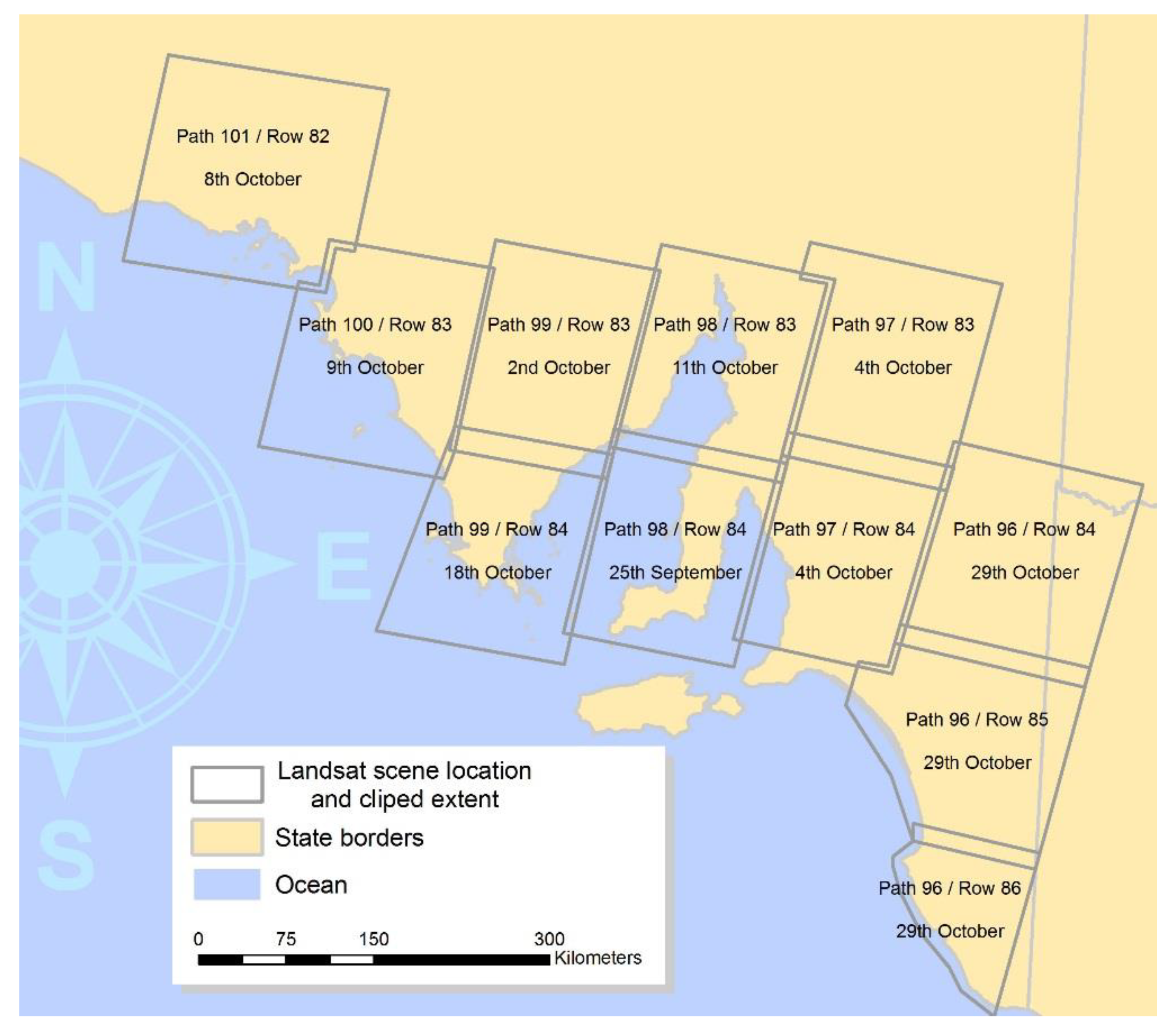
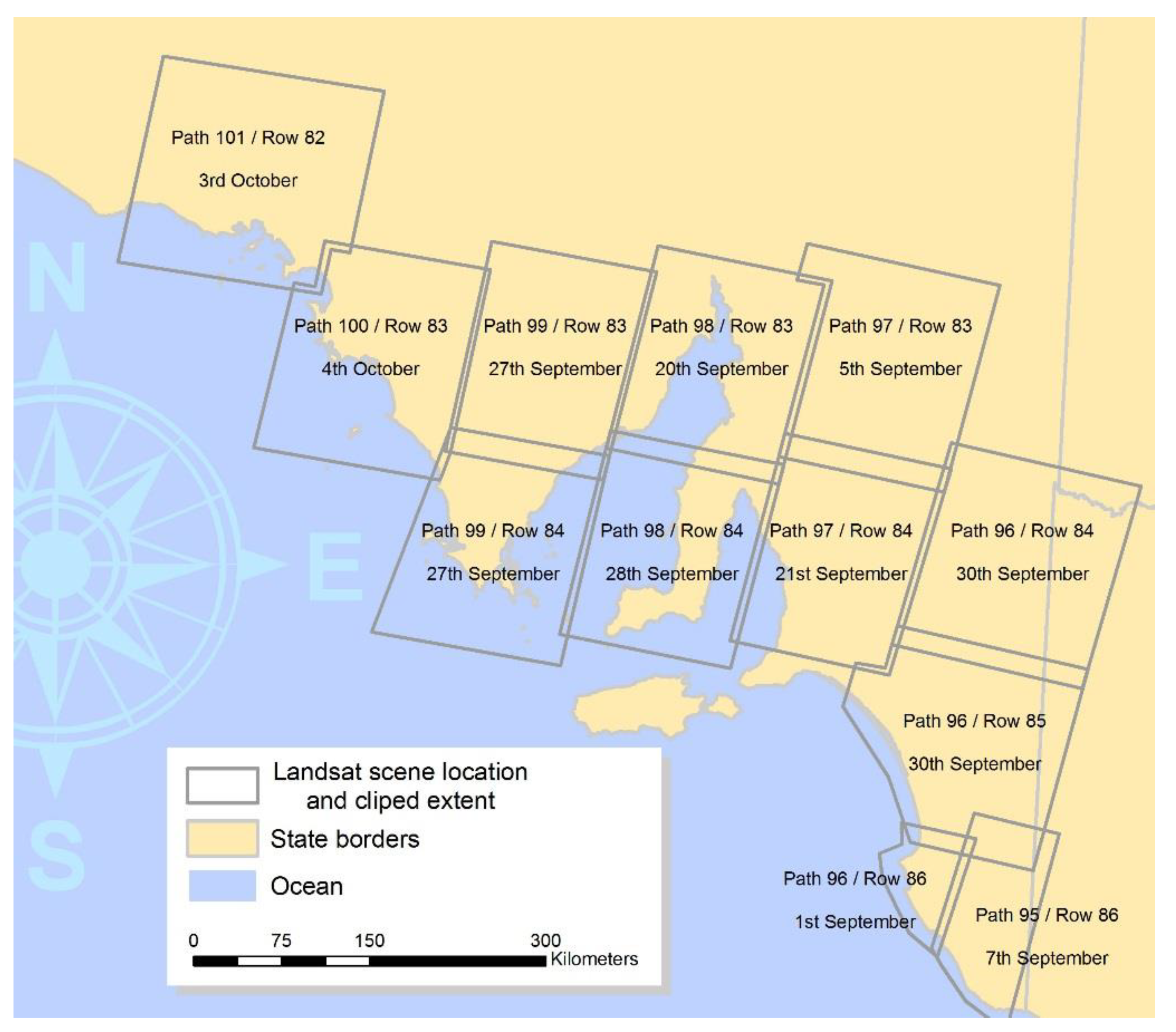
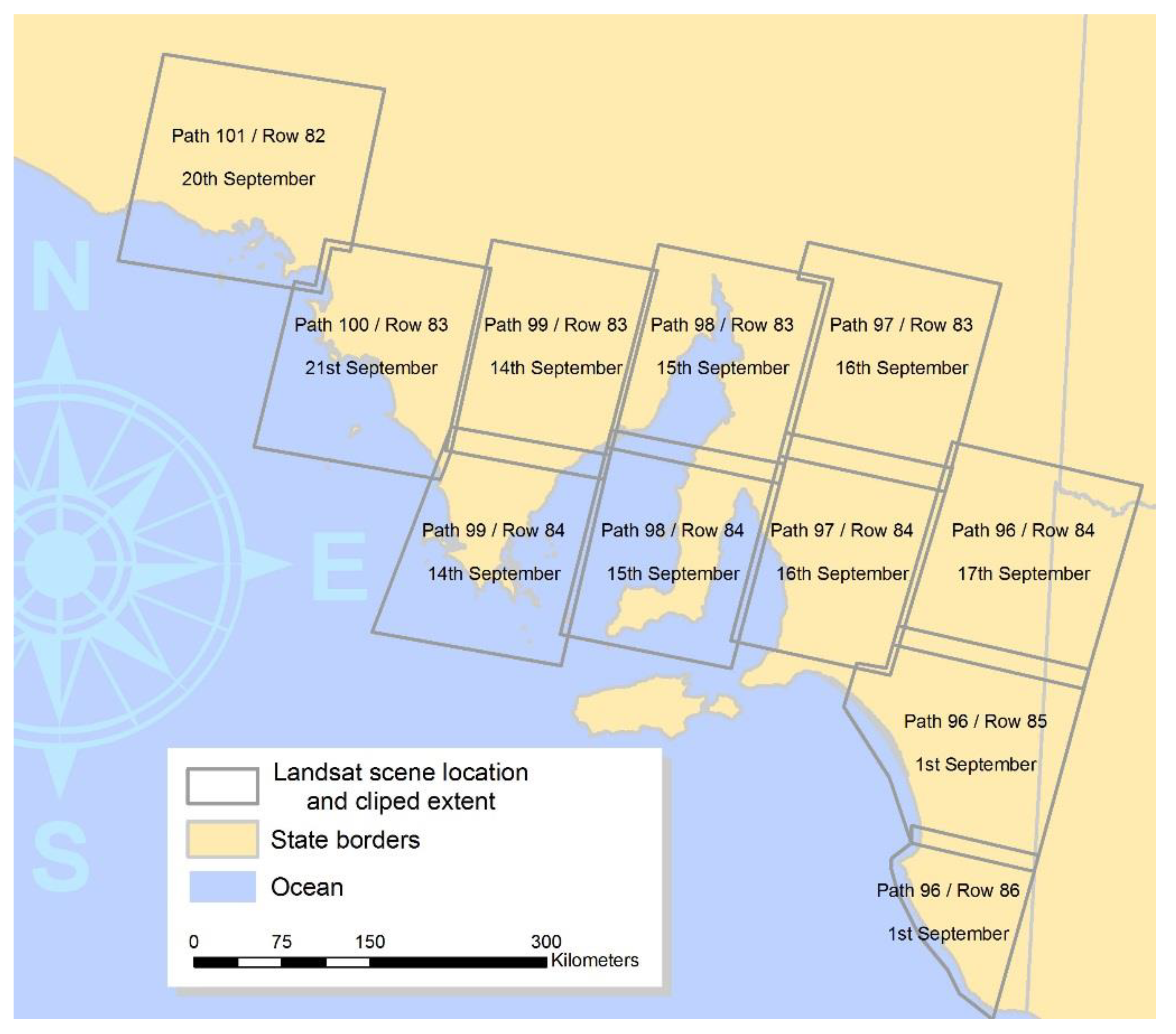
For the state-wide analysis, years under analysis were selected based on the availability of cloud-free images and the large spatial distribution of yield mapping files. A set of ten images from neighbouring satellite paths and rows were mosaiced together to form one image (Appendix A Figure A1, Figure A2 and Figure A3). This mosaic was created for each of the three years: 2004, 2005 and 2006. Choices of image dates within these ten images were as close to the month of September as possible but varied by path and row across the state.

2.3. Creation of the Broad-Scale, High-Resolution Yield Estimates

A four-step process was used to create the high-resolution geo-information that represented yield at a broad scale.

2.3.1. Step 1: Creating the Geographic Representation of Dryland Agricultural Fields across the YPA and the State-Wide Region

We created a spatial representation of dryland agricultural fields across the study areas using three polygonal and one rasterised dataset created by South Australian and Australian government authorities. We first overlaid two polygonal national [55] and state [56] land use datasets to geographically define the dryland cropping land use of South Australia. Native vegetation, which contaminates the spectral signatures of dryland cropping pixels, was removed from the representation by spatially extracting vegetation elements from the Australian National Vegetation Information System dataset rasterised to a 100 m resolution [57]. Finally, the South Australian cadastral database [58] was spatially overlayed onto the native-vegetation-free dryland cropping region representation to provide a basis to delineate individual field boundaries across the study areas. Using aerial photography, we further delineated field boundaries manually.

2.3.2. Step 2: Imagery

Step 2a: Crop Type Classification

To identify the annual spatial distribution of crop types defined as wheat, barley or other break crop types, we undertook a supervised classification approach using additional Landsat imagery collected between August and October. As wheat and barley are the predominate crops in the study areas, with a cropping of intensity of 51% and 26% of cropping area, respectively [50], we focussed on these crop types. A lack of detailed crop type information in 1999 and 2001 meant that the training and validation areas were only available from fields that were yield mapped. One farm within the YPA did have a long, detailed archive of data, and these data were randomly assigned to the training and validation areas based on a 50% breakup. A similar data assignment process was undertaken for later years for the YPA and the state-wide analysis, for which both crop type histories and yield mapping data were available for fields from different farms.
Within the training datasets, training signatures were extracted based on the field boundaries, minus a 30 m buffer to ensure that mixed boundary pixels were excluded. Classification was performed in ERDAS Imagine using the maximum likelihood decision rule. Post-classification likelihood thresholding was used to remove the 5% of pixels with the lowest probability of belonging to either the wheat, barley or other break crop types.

Step 2b: Aggregation of Crop Classification Results to Fields

In Australian agriculture, only one crop is predominately sown per field in one season. However, the Step 2a pixel-based method of classification created a speckled pattern of crop type classifications within specific field boundaries. We overlayed the individual field boundaries from the dryland cropping representation (Step 1) on the supervised classification to estimate the proportion of classified pixels to wheat, barley and other break crop types within each field. We then accessed agriculture statistics on the annual area planted with wheat and barley in 11 regions of South Australia to act as an inclusion or exclusion criterion [50]. Each field was then assigned to one of the 11 regions and sorted in ascending order based on the proportion of classified pixels to a crop type. Total field area was then calculated sequentially down the ranking. Cumulative annual field area totals were then matched to annual crop area statistics for each region to define the spatial distribution of crop types across the study areas.

Step 2c: Accuracy Assessment of Crop Type Discrimination

The accuracy of classification was tested against the validation datasets throughout the study areas over time (Appendix A Table A1). We calculated an overall assessment of classification accuracy measured by the sum of correctly classified fields divided by the total number of fields, as well as the yearly Kappa coefficient for both study areas. This Kappa statistic determines whether the results presented in the error tables were significantly better than a random result. Values lower than 40% indicate poor agreement, whereas values ranging from 40% to 80% represent moderate agreement.

Step 2d: Calculation of Normalised Difference Vegetation Index (NDVI)

NDVI was calculated for each study area image following the standard method, which is not detailed here. Crop-specific NDVI values were extracted from the distribution of wheat and barley fields across all years for both study areas identified in the crop type classification. This process defined the spatial distribution of NDVI values for wheat and barley crops across all years.

2.3.3. Step 3: Creation of Field Yield Maps

Step 3a: Field Yield Data Used for the YPA and State-Wide Analysis

High-resolution yield-mapped data were provided by SPAA. The volume and spatial distribution of yield data varied (Figure 1), particularly in the early years in which the adoption of yield mapping was low (Appendix A Table A1). We matched the year in which the yield-mapped data were collected to the years that corresponded to cloud-free imagery.

Step 3b: Yield Data Post Processing

Yield mapping data were run through post-processing error removal software [59]. The software removed errors associated with harvester dynamics, the collection of measurements to calculate grain yield, the global positioning system and the driving of the combine operator [60]. The implementation of such routines on these datasets produces more normally distributed yields than those observed in the raw datasets [38]. This process has been utilised in other studies in the Australian cropping environment [41,43,44].

Step 3c. Creation of Field Yield Maps

To establish yield estimates at the same spatial resolution as the Landsat imagery, all yield mapping datasets were interpolated using the Australian Centre for Precision Agriculture (ACPA) VESPER kriging software [61]. Wheat and barley grain yield surfaces were created at a grid resolution of 30 m using the ACPA yield mapping creation protocol [62]. The interpolation process produced a spatial structure for grain yield estimates across missing areas due to error removal and acted as a locational basis for spatial comparison of high-resolution yield values and satellite-based surrogate measurements for biomass.

Step 3d. Fine-Scale Yield Prediction and Validation

High-resolution yield-to-NDVI relationships were developed for wheat and barley crop types for both study areas. The 30 m pixels in the interpolated field yield maps were randomly divided into training and validation sets based on a 50:50 ratio, then matched with the corresponding NDVI values for that location. Power regression relationships were fitted to the data for both study areas. These relationships were then used to predict yields within the validation dataset based on each field’s array of NDVI values. Yield prediction accuracy was evaluated against the corresponding interpolated observed yields within the validation dataset with two efficiency criteria: the root mean square error (RMSE) and the Nash–Sutcliffe efficiency criterion (E). These efficiency criteria were chosen to provide an overall estimation of model accuracy. The RMSE value allows for the comparison of model prediction accuracy across models, as it normalises the prediction error to tonnes per hectare (t/ha) across varying yield distributions used in the validation process. The Nash–Sutcliffe efficiency criterion (E) is another well-established indicator of model prediction efficiency and is used to determine the prediction performance of the model compared to using the average yield value for prediction [63]. Values of E range from 1 (indicating a perfect model fit) to −∞, with values lower than zero indicating that the mean of the observed dataset would have been a better predictor than the model.
This process was followed to develop yield—NDVI relationships for (1) the annual crop-specific models; (2) the annual pooled crop type models which pool both the wheat and barley datasets, testing whether crop discrimination was necessary; (3) the global crop-specific models, which pool the annual yield data, testing whether accessing yield data annually was necessary and; (4) the global models, which pool both crop type and annual yield data from each year across each study region, testing whether crop discrimination and accessing yield data annually was necessary. We tested the ability of these generalised models to predict yield by comparing the magnitude of RMSE and the number of times the Nash–Sutcliffe efficiency criterion (E) value was greater than 0 when validated against the range of annual yield validation datasets.

2.3.4. Step 4: Creation of Broad-Scale, High-Resolution Geo-Information on Wheat and Barley Yield for the YPA and State-Wide Analysis

Step 4a: Extrapolation of Yields across the YPA and State-Wide Study Areas

Wheat and barley yield prediction models for each year (annual models) were applied to the corresponding crop-discriminated NDVI imagery in order to derive the spatial and temporal distributions of yields across both study areas.

Step 4b. Broad-Scale Annual Yield Prediction and Validation Using Agricultural Yield Statistics from Government Administrative Regions

The wheat and barley yields predicted across the state-wide study area were geographically separated into their corresponding government administrative regions [50]. Average wheat and barley yields were calculated for each of the 11 government administrative regions for the three years of the study. These regional yield averages were then compared to the reported annual yield statistics for each administrative region [50]. Based on this comparison, the Nash–Sutcliffe efficiency criterion (E) was calculated to determine model performance for each year. This acted as a test of the generalisability of the fine-scale yield–NDVI relationships to predict coarser-scale regional yields. This evaluation identified whether the high-resolution yield–NDVI relationships at the regional scale hold across areas where the yield mapping data for the model were not available.

Step 4c.: Coarse-Level Yield Prediction and Validation

To enable testing of the temporal generalisability of the yield–NDVI models at coarser scales, the 2005 empirical model was applied to the NDVI values for 2004 and 2006. Average regional predicted yield for each of the 11 administrative region was calculated by averaging the high-resolution yield predictions from the 2005 model within each of their corresponding regions. Average regional yield predictions were compared to the reported annual yield statistics for each administrative region [50] for 2004 to 2006. The Nash–Sutcliffe efficiency criterion (E) was calculated to determine the performance of the 2005 model to predict yield across the state over these two years.

3. Results

3.1. YPA and State-Wide Crop Type Classification Accuracy

Table 1 shows the overall crop discrimination accuracy and Kappa statistics for the YPA and state-wide analysis. For YPA, 1999, 2001 and 2007 showed good prediction accuracy with high overall accuracy and Kappa statistic values. These positive results reflect the fact that the majority of the validation data, especially for 1999 and 2001, was taken from one farm or from fields within close proximity. For the other years, the overall accuracy was moderate to poor for wheat and barley field prediction capability, with substantially lower Kappa statistics. For the state-wide analysis, the overall accuracy of the crop type classification for 2004, 2005 and 2006 was low (Table 1), with fewer than half of all wheat and barley fields mapped successfully across the South Australian dryland cropping region. These less reliable results demonstrate that the spectral signatures used in the crop type discrimination based on the choice and range of training data selected across the large study areas were not an accurate representation of the spectral signatures found in the set of validation data taken from across the large study areas. This is potentially due to the large variations in distances between field sites, which could bias the discrimination ability of the training dataset. Additionally, the large distances between validation datasets suggest that their field-level spectral signatures may also differ. These distances could be over 100 km in the YPA and potentially larger for the state-wide analysis.

3.2. Yield–NDVI Relationships and Prediction Accuracy for YPA and State-Wide Analyses

3.2.1. Evaluation of the Yield–NDVI Models for Wheat and Barley for the YPA

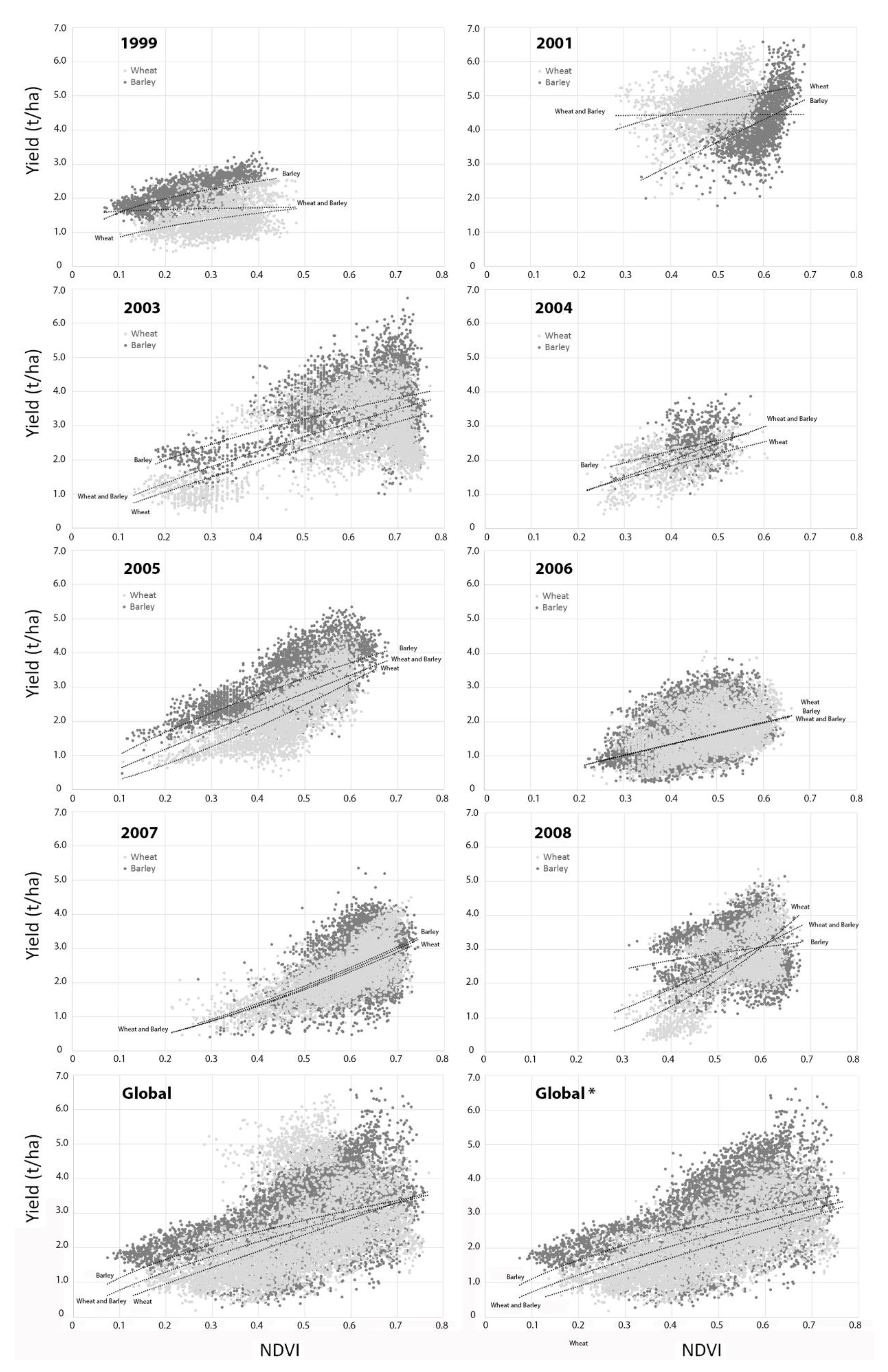
Figure 2 and Table 2 show the distribution, calibration and validation estimates for the annual and generalised empirical models investigating the relationship between yield and NDVI. Weak positive relationships were recorded for the wheat yield–NDVI associations in 1999, 2001 and 2006, with R2 values of less than 0.20. Relationships for the other four years were of moderate strength, with R2 values ranging between 0.23 and 0.56. Annual wheat models showed moderate yield prediction accuracy, with RMSE values ranging from 0.42 t/ha to 0.91 t/ha, representing 29% to 31% of average yield. All annual wheat models reported greater yield prediction capability than using the average value of the dataset (E > 0) alone, with E values ranging from 0.11 to 0.59. Barley yield–NDVI relationships also exhibited positive relationships, but R2 values were of low to moderate strength, with values ranging between 0.09 and 0.35. Annual barley models showed moderate yield prediction accuracy, with RMSE values varying from 0.3 t/ha to 0.8 t/ha. These values represented 14% to 26% of average yield for each year. All annual barley models showed greater yield prediction capability than using the average value of the dataset (E > 0) alone, with E values ranging from 0.002 to 0.47. These results suggest that the relationship between yield estimated at the end of the season via the yield mapping and NDVI, which is captured as a single image measurement mid-season, seems to hold. In these cases, low yield values are related to low NDVI values, and high yield values are related to high NDVI values. However, there were years in which yield was not related to NDVI. The years 1999 and 2001 show two contrasting trends, illustrating the limitations of the snapshot approach of the single-datapoint NDVI acquisition. In 1999, there was a narrow range of yield-mapped values related to low NDVI values (<0.4). In 2001, there was a range of high yield values between four and six t/ha related to a narrow range of NDVI values for 2001 (0.3–0.65). There may have been calibration issues with the yield mapping measurement collection in these early years of technology adoption, resulting in small ranges and high magnitudes in measured yield across the farm. Similarly, for the year 2006, when rainfall was constrained (Appendix A Table A1), we observed high NDVI values recorded in September and low yield values collected in December (Figure 2). This suggests a climate-constrained ending to the season, which impacted the final yield and therefore prediction capability.
Pooling both wheat and barley datasets (categorised as “pooled” in Table 2) for each year showed no relationships in the years 1999 and 2001, with Figure 2 demonstrating a near-linear model fit and Table 2 reporting negative E values. Better relationships were found for the six other years, with R2 values ranging between 0.16 and 0.38. The pooled annual 2004 model showed a better relationship than the single crop models for that year, driven by the relationship between barley yield and NDVI at higher values. RMSE varied between 0.51 to 0.91 t/ha, representing 24% to 38% of the average yield. The use of these models represents a small reduction in prediction accuracy compared to the annual crop type models.
Combining the annual datasets to form the “global” category in Table 2 demonstrated moderate relationships for wheat, barley, and wheat and barley (pooled) crop types for the global model. However, as we aggregated the data, the R2 values were reduced, ranging from 0.20 to 0.32, and the assessment of the prediction accuracy showed an increase in RMSE values to between 0.95 t/ha and 1.12 t/ha. These values equated to 32% to 46% of average yield, and E values still demonstrated reasonable model prediction. Given that the distribution of the wheat–NDVI relationship in 2001 substantially differed from all other distributions, we removed these estimates from the global model. This removal provided better relationships both in the wheat (with RMSE almost halved: 0.67 t/ha, representing 32% of average yield) and pooled models. Removing these data from the pooled model showed slightly better estimates of model calibration and validation when compared to the other global pooled crop type model (Table 2).

3.2.2. Evaluation of the Generalisability of the Models over Time

The predictive accuracy of each of the developed models was tested against single-year validation datasets made up of both wheat and barley yields (Appendix A Table A2). The 1999 and 2001 annual crop-specific and annual pooled crop type models provided poor generalisability, with the 1999 wheat and barley models providing accurate model predictions in only one (2006) and two years (2005 and 2008), respectively. In contrast, all other models had poor predictive accuracy when validated against the 1999 and 2001 validation datasets. Predictive accuracy for the 2003 to 2008 annual models varied, with the highest predictive accuracy for the 2004 barley model and the 2003, 2004 and 2005 annual pooled crop type models. These models demonstrated the ability to predict yield across four of the same years (2003, 2004, 2005 and 2008) with similar prediction accuracy and RMSE values. RMSE was above 0.8 t/ha for all validation years except for 2004 (<0.6 t/ha). The 2007 annual pooled crop type model was a reasonable predictor of yield for 2006, but the same model did not predict yield well for 2007. These results suggest that these models could only predict yield in the years in which the ranges of yield-to-NDVI relationships were similar, i.e., four out of the eight years.
The model performance of the global models in predicting yield over the eight years also varied. All models performed poorly in predicting yield for 1999 and 2001, with negative E values demonstrating that the average yield would be a better predictor than the developed models. The global wheat crop type and global pooled crop models provided moderate prediction accuracy for four out of the eight seasons, with the global pooled crop type model reporting slightly better results. Removal of the wheat yield for 2001 in the global wheat model resulted in a marked decline in accuracy and generalisability. Its exclusion in the global pooled crop type model provided a similar generalisability result; however, the prediction accuracy for 2007 became better than using the average (E = 0.12), but accuracy decreased for the year 2003 to no better than using the average yield value.

3.2.3. Evaluation of the State-Wide Yield–NDVI Models for Wheat and Barley

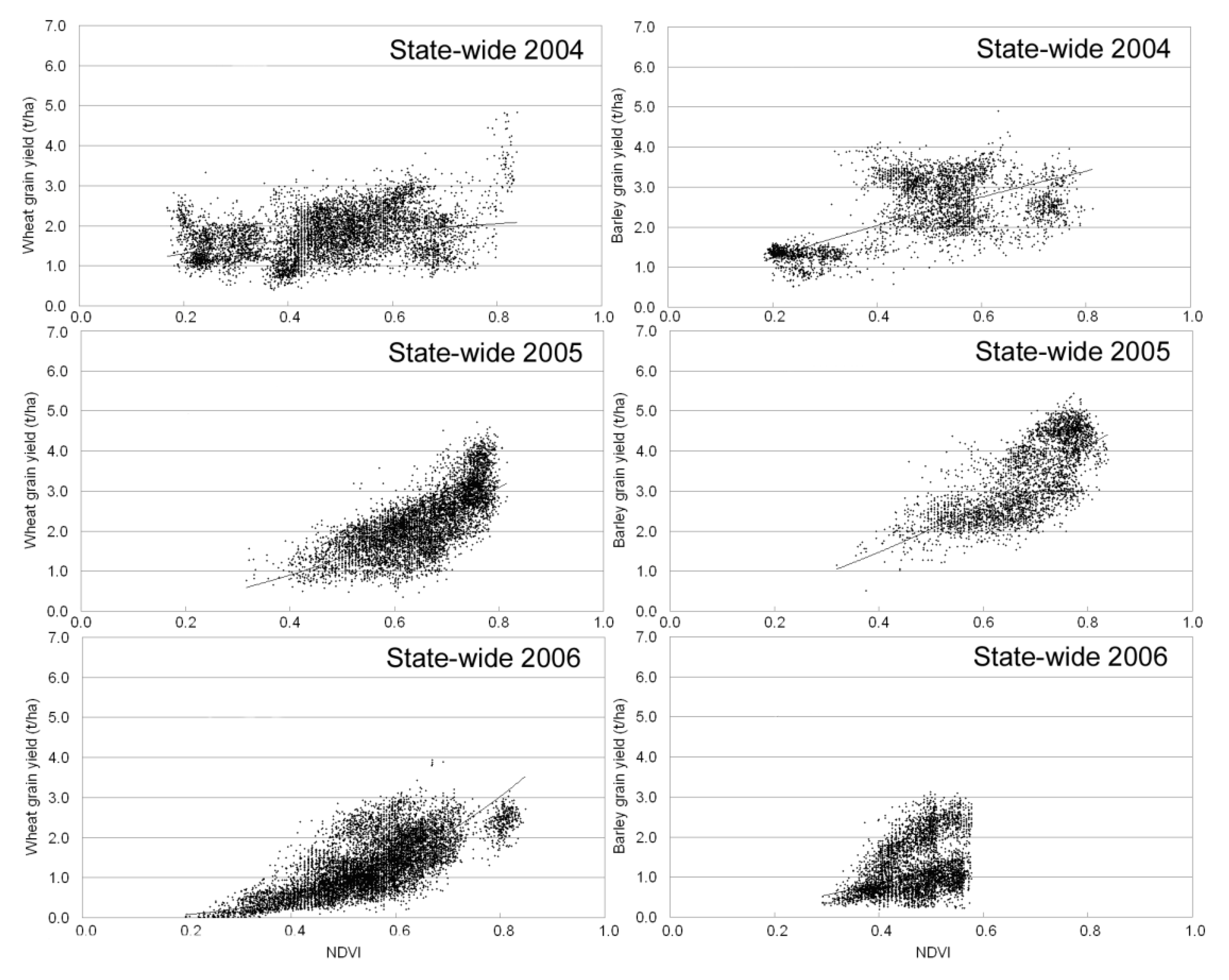
Figure 3 and Table 3 show a range of power relationships for wheat and barley yield values and NDVI for the state-wide analysis in 2004, 2005 and 2006. Weak relationships were recorded for wheat in 2004 and barley in 2006. Stronger relationships were recorded for wheat and barley in the other years, with R2 values ranging between 0.49 and 0.60. It is noteworthy to report that there are no NDVI values for barley greater than 0.6 in 2006 for the mosaicked imagery. The distributions of yield–NDVI values for the range of imagery selected for the 2004 state-wide analysis proposes a model with a near-linear relationship (Figure 3). This relationship substantially differs from the other years in the state-wide analysis and the YPA models. Extrapolation of the accuracy of the power models against their validation datasets showed that predictive power was moderate, especially for barley in 2004, wheat and barley in 2005 and wheat in 2006. However, as with the yield–NDVI relationship strength, predictive power was low for wheat in 2004 and barley in 2006. RMSE values ranged from 0.52 t/ha for wheat in 2004 to 0.78 t/ha RMSE for barley in 2005, representing 26% to 50% of average yield. The high relative prediction error (50%) in 2006 was caused by the existence of low yield and low NDVI values in that year.
Pooling the annual crop type data showed moderate yield–NDVI relationships, with R2 values ranging between 0.25 and 0.45. Validation of the models highlighted that RMSE was between 0.69 t/ha and 0.85 t/ha, representing 26% to 66% of average yield. This error was higher than that reported for the crop-specific models.

3.2.4. Evaluation of the Generalisability of the State-Wide Yield–NDVI Models

The yield models for 2005 provided the best annual predictor of yields. We chose the models for this year to undertake interannual comparisons using the 2004 and 2006 state-wide validation datasets (Table 3). These models showed the poor predictive capability and therefore the poor generalisability of the 2005 model. Here, average yield was a better predictor of yield in all cases, except for wheat in 2006, for which the reported E value was 0.26. Pooling the crop types together for the 2005 model showed no significant gain in accuracy, with negative E and high RMSE values.

3.3. The Creation of Geo-Information Representing Broad-Scale, High-Resolution Yield Estimates for the State-Wide Study Area

3.3.1. The Annual Spatial Representations of Wheat and Barley Yields across the State-Wide Study Area

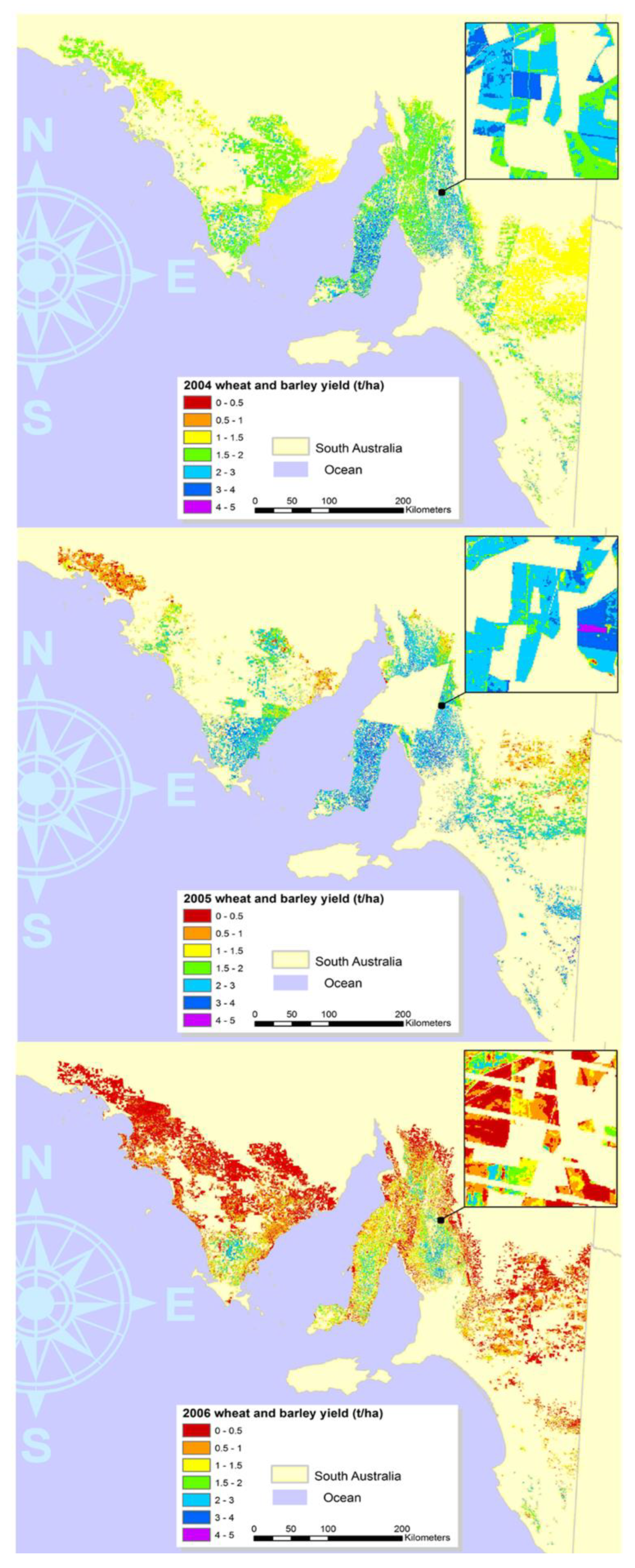
Figure 4 shows an example of the predicted yield from the extrapolated empirical models for the state-wide analysis for 2004 to 2006. Broad trends in yield variation can be seen across the state; the insets within the maps show the spatial pattern of yield within and across fields due to the high resolution of the data used. For 2004, yield varied from 1.0–4.0 t/ha, with higher yield estimates clustered in the YPA study region. A defined line through the eastern side of the image shows yield differences caused by the mosaicking of different image dates, which were 25 days apart due to cloud cover. Yield estimates for 2005 showed greater yield variation, with values ranging between 0.5 and 5.0 t/ha. A major proportion of the middle of the 2005 state-wide image was removed due to extensive cloud cover. The inset shows the high degree of spatial variation of yield, with some fields with yields varying from 1.5 to 4.0 t/ha within their boundaries. Finally, yield estimates for 2006 showed that a significant part of the state had predicted yields of less than 1.0 t/ha. Yield did vary with this season, with some fields within the inset having predictions of between 0.5 and 3.0 t/ha within their boundaries. Also apparent in this inset is the interleaving of missing values caused by the scan line problem associated with the Landsat ETM+ sensor after July 2003.

3.3.2. Evaluation of the Broad-Scale Annual Yield Predictions

The scaled-up annual wheat and barley fine-resolution yield predictions compared favourably with the reported agricultural statistics at the administrative region level (Figure 5A). Annual yields are observed near the one-to-one line for predicted versus reported yields. Yields for 2004 and 2006 had the greatest dispersion around the one-to-one line. Higher yields were predicted for 2005, whereas lower yields were predicted for 2006. The Nash–Sutcliffe efficiency criterion (E) values for 2004 and 2006 were moderate, at around 0.35, whereas for 2005, E was around 0.65 (Figure 5C).
We used the 2005 model to test the generalisability of the model to predict yield estimates for the other two years. Yield predictions based on the 2005 model at the administrative region level for 2004 and 2006 all fall close to the one-to-one line for predicted versus reported yields (Figure 5B). This indicates little bias at this regional scale. This point cloud is also very similar to the distributions derived using the annually derived yield–NDVI relationships (Figure 5A). Interestingly, E shows a better fit when yields for these years are predicted from 2005 crop type models compared to those predicted by the annual models (Figure 5C): E for 2004 is now above 0.4, and for 2006, E is above 0.5. This is due to the wider distribution of NDVI and yield values in 2005 compared to a smaller range of values for 2004 and 2006. In addition, model efficiency was further increased when predicted and observed data pairs from “all years” were aggregated together, providing a greater range of values (Figure 5C).

4. Discussion

In this paper, we described the development and extrapolation of simple models at a resolution we considered appropriate (in this case, 30 m pixels) to support agricultural decisions of landholders and their potential spatial allocation on farm. This information must be able to demarcate marginal land where land use change can occur from those areas that produce higher yields where land use change should be reconsidered. Trust in the information that underlies these decisions is also critically important. Landholders’ trust is likely to be higher in geo-information data sources that they are familiar with using, such as yield mapping and satellite imagery to inform land management decisions [42]. Given that some trust has already been established, the usefulness of our approach is determined by the calibration and validation results of the selected models. We investigated a number of strategies to determine which models could be operationalised, as well as the accuracy that is inherent in these approaches. The annual crop-specific models provided the most reasonable calibration (R2 ranged from 0.003 to 0.56), and their validation results demonstrated superior prediction of yield compared to using average annual yield alone for yield prediction (E > 0) in the majority of cases. The average RMSE of the annual crop-specific models was 0.61 t/ha, with a statistical range of between 0.3 and 0.91 t/ha. These results are comparable to those of studies undertaken in north eastern Australia [45] and Western Australia [44]. However, the RMSE was higher than that reported in another study [46]—a median RMSE of 0.31 t/ha and standard deviation of 0.15 t/ha. This difference may be explained by a lack of statistical range in their data, as yearly observed yield was reported as three tonnes per hectare in only five of the 17 years reporting pixel-based yields. It is difficult to determine whether the created geo-information is justifiable for its use in the decision-making process based on RMSE. Some insight into its applicability was suggested by Kamir et al. (2020) [34], who proposed that their resulting RMSE (0.55 t/ha at the (250 m) pixel level) had a level of accuracy that was fit for the purpose because it was less than the size of the yield gap in their study region. They cited one study [64], in which the estimated yield gap over the whole Wimmera region of Victoria varied annually from 0.63 to 4.12 t/ha, with an average of 2.00 t/ha. Using this evaluation metric suggests that the bulk of our annual crop type models are also fit for purpose.
In order to operationalise these annual crop type models to predict crop yields across the YPA, we undertook crop type discrimination to identify which fields grew wheat and barley crops—the most dominate crop types in the region. We found that apart from 1999 and 2001, which used data from one farm, the overall crop discrimination accuracy for these two crops was generally above 50%. However, the Kappa coefficient showed moderate agreement in only half of the years under investigation. This means that we can only identify differences in crop types at the field level in specific years. This fluctuation in yearly discrimination results highlights the limitation of using spectral information from one yearly image taken in the August to September time period. Differentiation between crops is a challenge, especially in study areas that are more heterogeneous than ours. Methods that utilise the spatial and temporal differences in crop phenology [65,66] may be a first step to improve discrimination accuracy. In future analysis of larger regions, the use of machine learning algorithms to map specific crop types by dividing large regions into smaller regions to reduce the inherent intra-class variability of crop type discrimination [67,68] may prove a more effective crop discrimination technique.
Given the yearly variation in crop discrimination accuracy, we investigated whether we needed to spatially discriminate between wheat and barley crops by evaluating the benefit of aggregating the annual crop-specific models into annual pooled crop type models. With the exception 1999 and 2001, the models performed slightly worse than the annual crop-specific models (R2 ranged from 0 to 0.39, with an average RMSE of 0.70 t/ha and a statistical range of between 0.51 and 0.91 t/ha). Thus, a small trade-off in prediction accuracy is involved when both crop types are aggregated together. However, the reported RMSE values are close to the evaluation metric highlighted above [34], suggesting that these models were also fit for purpose. This suggests that there may not be a need to discriminate between these dominate crop types at the field level. However, crop type discrimination would still need to be conducted in order to differentiate between these dominate crops and other break crop types planted in the same season. Discrimination is needed so that the annual pooled crop type models can be geographically applied across the study area.
Generalised global models were also generated to determine whether there is a need to access yield data annually and discriminate between dominate crop types. The aggregation of yield data over eight years for the crop-specific and pooled crop type models provided reasonable calibration and validation results; however, RMSE was higher than both the annual models. Interestingly, when we removed what we believed was an erroneous dataset for wheat in the year 2001, the calibration and validation results against the wheat validation dataset for the global wheat crop type model improved substantially. Importantly, this shows the influence of one year’s data on the results of the global models.
We further tested whether the annual crop-specific, pooled crop type, global crop-specific and global pooled crop type models could provide robust predictive capacity across different years. We evaluated the potential generalisability of these models by recording how many times the Nash–Sutcliffe efficiency criterion (E) was greater than 0. The Nash–Sutcliffe efficiency criterion (E) is used to determine the predictive performance of a model compared to using the average yield value for prediction [63]. Overall, these results suggest that the majority of our annual crop-specific yield models poorly predict yield when validated against the annual validation datasets in which wheat and barley yields were combined. This is not that surprising, given the different yield–NDVI relationships of these crop types over time. The annual pooled crop type models provided better prediction accuracy than the annual crop-specific models, with the 2003, 2004 and 2005 models predicting yield in 2003, 2004, 2005 and 2008 better than the average yield estimate (E > 0). Given that there were some trends in their generalisability, we developed global pooled crop type and global models incorporating all data, which removed the need for continual access to annual yield data and crop type discrimination. The global wheat crop-specific model and the global pooled crop type models predicted yields better than the average yield in 2003, 2004, 2005 and 2008. The results of validation criteria from the global models were similar to those generated from the annual crop-specific models. Overall, the annual pooled crop type and global models may provide some benefit in the operationalisation of this methodology. Their RMSE were marginally higher than the annual pooled crop type models in the four years in which they achieved better predicted performance than the average. However, there were years—in particular, 2006 and 2007—in which the yield–NDVI relationships were not maintained; as such, the annual models performed much better. It also must be noted that the higher RMSE values generated from the annual crop-specific and global models suggest that these models might not be fit for the purpose of accurately predicting yield in some years, given the RMSE evaluation metric [34]. This indicates that accurate crop discrimination might be needed for this approach to be useful.
These results show what can be achieved through the use of a minimal dataset and simple models to predict yield at a high resolution over a broad region. Both the dataset and models utilised can be extended in their complexity to possibly provide incremental increases in model accuracy and reductions in error. Recent studies have utilised the multidimensionality of remotely sensed imagery and the data fusion of different sensors [45,46,47,48]. These studies have shown an increased efficacy of models using individual spectral bands rather than vegetation indices, multiple timings of imagery that integrate changes over the whole growing season at different locations and the application of other spatial data that further account for localised conditions to better estimate yield. Several studies have shown an increase in model performance utilising more complex modelling techniques [46,47], for example, the benefits of machine learning algorithms over traditional regression models [47]. These models are less data-intensive and may be of additional benefit in regions where yield mapping data are sparse. These algorithms may perform better when incorporating environmental variables, as they can identify and unpack relationships between explanatory variables to account for confounding factors that can reduce accuracy. These proposed methods also have the ability to manage multivariate data relationships rather than the univariate relationships generated through traditional regressions. Another methodological advancement is the extension of tradition regression to linear mixed-effects models [45,46]. This approach describes the simple general model through fixed-effect coefficients similar to the traditional regression models and then incorporates spatial and temporal variations in soil conditions, farm management practices and climate through local corrections from random-effects coefficients calculated from different fields, farms and years.
Our second objective was to test the spatial generalisability of the proposed methodology to the state-wide agricultural region. We achieved reasonable results for prediction of yield across the state, with the annual crop-specific models producing the best results, whereas pooling of the crop types once again produced slightly higher RMSE results. This is encouraging, given that we utilised yield data from geographically disperse farms across the state and single satellite images across different time periods for the period of August to September. However, this snapshot approach of stitching together different imagery dates does produce application issues. For example, the distribution of the yield-to-NDVI relationship for barley (Figure 3) developed across different dates of imagery for 2004, highlighting that different relationships do exist across the state. This is caused by geographic differences in climate–soil interactions in the same growing period and year. This reinforces our previous proposal that better techniques may be available to create these state-wide estimates.
We found that, as in other studies [48,49,69] in which high-resolution estimates of crop yield were created, our models can be interpreted as robust compared to a validation set made up of agricultural yield statistics reported at the aggregated administrative region level. This demonstrates that our models predict yield relatively well in areas where we did not have access to yield data. However, these results are misleading in terms of validating the models’ accuracy. As found in regional crop modelling studies, compensating errors may occur, with higher yields offsetting lower yields at the regional administrative level, and potentially large errors may still occur at higher resolutions [25,29]. We found that this situation occurred when we evaluated the models at the more appropriate pixel-level resolution. Models became less suitable for use, with E values becoming negative for most models. This reduction in yield prediction accuracy when compared to finer-resolution validation data has also been shown by others [48,49,70]. For example, one study [48] found that validation of the model using county-scale data produced an R2 of 0.63 and an RMSE of 0.40 t/ha, whereas using a pixel-scale validation dataset resulted in an R2 of 0.27 and an RMSE of 0.96 t/ha. Therefore, if the purpose of the study is to create geo-information at a high resolution over a broad extent, then the models must be evaluated at a comparative spatial resolution—in this case, at the pixel level.
Extrapolation of models requires high-accuracy crop discrimination; however, extending the snapshot approach to crop discrimination across this region provided very poor results. Clearly, a new approach is needed if we are to identify differences in crop rotations and land uses in a region where rainfall varies from 250 mm to 600 mm causes spatial variations in climate, crop phenology and agricultural land use. In this study, we manually created the boundaries; however, newer methods using a deep learning approach provide a more automated process to identify field boundaries in larger regions [71,72,73]. The second advancement needed would be the differentiation of crop types at the field level across extremely large regions. Creating such spatial infrastructure has previously required large governmental investment, such as for the cropland data layer in the USA [74]. However, understanding the benefit of this type of spatial infrastructure to the public good means that other countries such as Australia are proposing to [75] or have already followed suit [76,77].
In this study, we combined yield mapping data and NDVI from Landsat imagery over eight years, reaffirming the potential of this methodology to create high-resolution geo-information about yield at broad, regional scales. The data used were from 1999 to 2008 but enabled us to evaluate the effect on the predictive accuracy of generalising these models, test the ability to operationalise them over large agricultural regions and generate an important historical archive of geo-information that is reliant on the early adopters of yield mapping technology. Historical trends rely on data being available before issues emerge in the future. For example, CO2 and temperature records are being increasingly referenced to quantify the extent and causes of climate change [78,79]. With the future pressures of climate change on agriculture, the potential geo-information datasets created from the application of these methods will be valuable to decision makers in the future.
One of the main criticisms of this methodology is that it requires access to a large range of in situ measurements both at the field level from yield mapping and at the regional level from the satellite sensor. This criticism is becoming less applicable in both cases as more contemporary data are being collected to create a longer-term historical archive of crop yield trends to inform decision making. Adoption of yield mapping technology has slowly increased worldwide [42]. In Australia, adoption has been increasing, with surveyed rates rising from 26% of a progressive farm group [80] to 51% of respondents in cropping industries reporting that they collected yield mapping data [81]. Yield mapping information has also become more accessible through grower, research and governmental partnerships. Large numbers of field years within farms have been used in the UK [47], in regions within and across Australia [45,46,70] and across different farms and states in the US [48,49,82]. Complementing this increase has been the mostly free access to the ever-increasing long-term archive of global Landsat observations available through the Google Earth Engine [83], the United States Geological Survey (USGS) and country-specific providers. This study demonstrates the feasibility of creating a catalogue of past yield performance from which more spatially in-depth productivity analysis can be undertaken across farms and catchments over time [41,43]. This geo-information can serve as a critical evidence base for the identification of management of areas for farm management with precision agriculture technology [82] and the allocation of land for climate change mitigation and adaptation strategies [84] at a finer resolution than currently available at the broad regional level.

5. Conclusions

Historical high-resolution geo-information on yield is needed to optimise current management practices and to prevent future financial losses caused by maladaptation to climate change. We have shown that the models calibrated annually were the best predictors of this geo-information across a large cereal cropping area but less so for the whole South Australian cropping region. However, this approach can only be useful if a more accurate method is identified to discriminate crop types across large study areas. Generalisation of these models to remove the need for crop type discrimination and the continual access to annual yield data showed some benefit in years in which the yield–NDVI relationship had similar ranges. However, this approach was associated with a decrease in prediction capacity, making these generalised models possibly not fit for the intended purpose in some years. While the accuracy of the models varied, the results reported in this paper show the potential of geo-information to fill an information void. Future advancements in crop discrimination and modelling methodology and the acquisition of more up-to-date datasets could potentially enable the proposed approach to create an even more powerful evidence base that can inform current management decisions and future on-farm land use in cropping regions worldwide.

Author Contributions

Conceptualization, Greg Lyle and Bertram Ostendorf; Formal analysis, Greg Lyle, Kenneth Clarke, Adam Kilpatrick and David McCulloch Summers; Funding acquisition, Bertram Ostendorf; Methodology, Greg Lyle, Kenneth Clarke, Adam Kilpatrick, David McCulloch Summers and Bertram Ostendorf; Writing—original draft, Greg Lyle; Writing—review and editing, Greg Lyle, Kenneth Clarke, Adam Kilpatrick, David McCulloch Summers and Bertram Ostendorf All authors have read and agreed to the published version of the manuscript.

Funding

This research was funded by the Natural Resource Management (NRM) Research Alliance.

Data Availability Statement

Not applicable.

Acknowledgments

The authors would like to acknowledge the growers within and the Society of Precision Agriculture Australia (SPAA) for access to their yield mapping datasets.

Conflicts of Interest

The authors declare no conflict of interest. The funders had no role in the design of the study; in the collection, analyses or interpretation of data; in the writing of the manuscript; or in the decision to publish the results.

Appendix A

Table A1. Number of fields by year and crop type used in the accuracy assessment of the Yorke Peninsula and State-Wide regions.
YearRainfall (March–October (mm))WheatBarleyTotal
19992745712
20013756410
2003257271239
2004240251136
2005278393069
2006165203068
2007246222042
2008252334073
State-wide 2004 331750
State-wide 2005 5546103
State-wide 2006 414384
Table A2. Generalisability of the annual crop-specific, annual pooled crop type and global yield prediction models based on root mean square error (RMSE) in t/ha and the Nash–Sutcliffe efficiency criterion (E) for each annual pooled crop type validation set.
Annual Validation Sets Incorporating Pooled Wheat and Barley Yield Datasets
1999 2001200320042005200620072008Model Generalisability (Count)
ModelTypeRMSEERMSEERMSEERMSEERMSEERMSEERMSEERMSEE
1999Wheat0.72−0.842.83−14.601.68−1.930.77−0.661.23−0.450.630.110.92−0.521.38−1.391
1999Barley0.69−0.691.90−6.060.99−0.030.67−0.240.920.191.15−1.960.78−0.090.860.082
1999Pooled0.53−0.022.86−14.951.81−2.400.73−0.481.22−0.440.670.001.03−0.911.43−1.540
2001Wheat2.25−17.040.84−0.392.00−3.192.46−15.812.31−4.153.08−20.302.68−11.892.21−4.870
2001Barley0.80−1.261.07−1.241.46−1.201.10−2.331.01−0.111.82−6.411.90−5.471.31−1.160
2001Pooled2.69−24.850.72−0.011.52−1.402.36−14.422.25−3.882.87−17.432.10−6.931.81−3.120
2003Wheat0.75−0.992.18−8.311.04−0.130.540.200.900.210.80−0.420.670.200.92−0.063
2003Barley0.81−1.341.42−2.920.910.130.93−1.400.990.061.52−4.221.21−1.620.95−0.122
2003Pooled0.65−0.501.86−5.770.910.140.550.160.820.361.04−1.440.86−0.320.830.144
2004Wheat0.75−1.002.32−9.531.15−0.370.570.100.960.110.73−0.200.640.280.99−0.243
2004Barley0.60−0.281.97−6.590.970.020.560.140.860.291.01−1.290.75−0.010.850.094
2004Pooled0.76−1.082.01−6.850.950.050.510.250.840.320.90−0.800.79−0.110.850.094
2005Wheat0.93−2.121.98−6.661.01−0.060.560.150.850.300.87−0.700.91−0.490.860.073
2005Barley0.74−0.951.33−2.481.02−0.080.90−1.260.950.141.54−4.341.38−2.421.01−0.211
2005Pooled0.70−0.751.69−4.600.940.070.580.060.790.401.14−1.941.07−1.050.850.104
2006Wheat1.03−2.802.83−14.661.55−1.510.90−1.251.29−0.610.630.110.81−0.181.37−1.341
2006Barley1.04−2.852.84−14.831.57−1.560.91−1.301.31−0.640.630.110.82−0.211.38−1.381
2006Pooled1.04−2.872.84−14.781.56−1.530.91−1.301.30−0.630.630.110.82−0.201.37−1.371
2007Wheat1.17−3.892.64−12.621.28−0.710.89−1.21.23−0.450.630.100.630.291.20−0.822
2007Barley1.13−3.542.53−11.531.20−0.510.82−0.861.16−0.290.640.090.610.331.12−0.582
2007Pooled1.16−3.842.60−12.161.25−0.610.87−1.091.20−0.390.640.100.620.311.17−0.712
2008Wheat1.29−4.902.20−8.491.26−0.650.82−0.861.07−0.090.76−0.280.99−0.770.98−0.200
2008Barley0.81−1.321.70−4.650.920.130.80−0.790.960.111.33−2.950.91−0.480.860.083
2008Pooled0.92−2.021.98−6.631.00−0.050.550.160.850.310.87−0.710.91−0.470.860.083
Global Wheat0.80−1.282.13−7.841.00−0.040.540.190.880.240.81−0.480.710.110.890.0034
Global *Wheat0.84−1.532.36−9.871.15−0.370.61−0.041.000.050.70−0.090.630.301.01−0.292
GlobalBarley0.63−0.431.78−5.170.900.160.65−0.160.860.291.18−2.100.88−0.400.830.133
GlobalPooled0.64−0.471.97−6.570.950.070.530.230.840.330.97−1.110.77−0.060.850.104
Global *Pooled 0.66−0.552.09−7.501.00−0.050.520.260.870.280.88−0.750.700.120.880.034
* Wheat yield and NDVI estimates for 2001 were excluded from the model.
Figure A1. Mosaicked Landsat scene dates for the 2004 growing season.
Ijgi 12 00050 g0a1
Figure A2. Mosaicked Landsat scene dates for the 2005 growing season.
Ijgi 12 00050 g0a2
Figure A3. Mosaicked Landsat scene dates for the 2006 growing season.
Ijgi 12 00050 g0a3

References

  1. Erb, K.H.; Haberl, H.; Plutzar, C. Dependency of global primary bioenergy crop potentials in 2050 on food systems, yields, biodiversity conservation and political stability. Energy Policy 2012, 47, 260–269. [Google Scholar] [CrossRef] [PubMed]
  2. Smith, P.; Haberl, H.; Popp, A.; Erb, K.H.; Lauk, C.; Harper, R.; Tubiello, F.N.; Pinto, A.D.; Jafari, M.; Sohi, S.; et al. How much land-based greenhouse gas mitigation can be achieved without compromising food security and environmental goals? Glob. Chang. Biol. 2013, 19, 2285–2302. [Google Scholar] [CrossRef] [PubMed]
  3. Shirsath, P.B.; Aggarwal, P.K. Trade-Offs between Agricultural Production, GHG Emissions and Income in a Changing Climate, Technology, and Food Demand Scenario. Sustainability 2021, 13, 3190. [Google Scholar] [CrossRef]
  4. Hoffmann, H.; Zhao, G.; van Bussel, L.G.J.; Enders, A.; Specka, X.; Sosa, C.; Yeluripati, J.; Tao, F.; Constantin, J.; Raynal, H.; et al. Variability of effects of spatial climate data aggregation on regional yield simulation by crop models. Clim. Res. 2015, 65, 53–69. [Google Scholar] [CrossRef]
  5. Doelman, J.C.; Stehfest, E.; Tabeau, A.; van Meijl, H.; Lassaletta, L.; Gernaat, D.; Hermans, K.; Harmsen, M.; Daioglou, V.; Biemans, H.; et al. Exploring SSP land-use dynamics using the IMAGE model: Regional and gridded scenarios of land-use change and land-based climate change mitigation. Glob. Environ. Chang. 2018, 48, 119–135. [Google Scholar] [CrossRef]
  6. Cao, M.; Zhu, Y.H.; Quan, J.L.; Zhou, S.; Lue, G.; Chen, M.; Huang, M.X. Spatial Sequential Modeling and Predication of Global Land Use and Land Cover Changes by Integrating a Global Change Assessment Model and Cellular Automata. Earths Future 2019, 7, 1102–1116. [Google Scholar] [CrossRef]
  7. Roe, S.; Streck, C.; Beach, R.; Busch, J.; Chapman, M.; Daioglou, V.; Deppermann, A.; Doelman, J.; Emmet-Booth, J.; Engelmann, J.; et al. Land-based measures to mitigate climate change: Potential and feasibility by country. Glob. Chang. Biol. 2021, 27, 6025–6058. [Google Scholar] [CrossRef]
  8. Alexander, P.; Rabin, S.; Anthoni, P.; Henry, R.; Pugh, T.A.M.; Rounsevell, M.D.A.; Arneth, A. Adaptation of global land use and management intensity to changes in climate and atmospheric carbon dioxide. Glob. Chang. Biol. 2018, 24, 2791–2809. [Google Scholar] [CrossRef]
  9. Byers, E.; Gidden, M.; Leclere, D.; Balkovic, J.; Burek, P.; Ebi, K.; Greve, P.; Grey, D.; Havlik, P.; Hillers, A.; et al. Global exposure and vulnerability to multi-sector development and climate change hotspots. Environ. Res. Lett. 2018, 13, 055012. [Google Scholar] [CrossRef]
  10. Audsley, E.; Trnka, M.; Sabate, S.; Maspons, J.; Sanchez, A.; Sandars, D.; Balek, J.; Pearn, K. Interactively modelling land profitability to estimate European agricultural and forest land use under future scenarios of climate, socio-economics and adaptation. Clim. Chang. 2015, 128, 215–227. [Google Scholar] [CrossRef] [Green Version]
  11. Holman, I.P.; Brown, C.; Janes, V.; Sandars, D. Can we be certain about future land use change in Europe? A multi-scenario, integrated-assessment analysis. Agric. Syst. 2017, 151, 126–135. [Google Scholar] [CrossRef] [PubMed]
  12. Grundy, M.J.; Bryan, B.A.; Nolan, M.; Battaglia, M.; Hatfield-Dodds, S.; Connor, J.D.; Keating, B.A. Scenarios for Australian agricultural production and land use to 2050. Agric. Syst. 2016, 142, 70–83. [Google Scholar] [CrossRef]
  13. Bryan, B.A.; Nolan, M.; McKellar, L.; Connor, J.D.; Newth, D.; Harwood, T.; King, D.; Navarro, J.; Cai, Y.; Gao, L.; et al. Land-use and sustainability under intersecting global change and domestic policy scenarios: Trajectories for Australia to 2050. Glob. Environ. Chang. 2016, 38, 130–152. [Google Scholar] [CrossRef]
  14. Ahmad, Q.; Biemans, H.; Moors, E.; Shaheen, N.; Masih, I. The Impacts of Climate Variability on Crop Yields and Irrigation Water Demand in South Asia. Water 2021, 13, 50. [Google Scholar] [CrossRef]
  15. Lungarska, A.; Chakir, R. Climate-induced Land Use Change in France: Impacts of Agricultural Adaptation and Climate Change Mitigation. Ecol. Econ. 2018, 147, 134–154. [Google Scholar] [CrossRef]
  16. Gaal, M.; Quiroga, S.; Fernandez-Haddad, Z. Potential impacts of climate change on agricultural land use suitability of the Hungarian counties. Reg. Environ. Chang. 2014, 14, 597–610. [Google Scholar] [CrossRef]
  17. Shirsath, P.B.; Aggarwal, P.K.; Thornton, P.K.; Dunnett, A. Prioritizing climate-smart agricultural land use options at a regional scale. Agric. Syst. 2017, 151, 174–183. [Google Scholar] [CrossRef]
  18. Nadeem, F.; Jacobs, B.; Cordell, D. Mapping agricultural vulnerability to impacts of climate events of Punjab, Pakistan. Reg. Environ. Chang. 2022, 22, 66. [Google Scholar] [CrossRef]
  19. Jeong, J.S. Design of spatial PGIS-MCDA-based land assessment planning for identifying sustainable land-use adaptation priorities for climate change impacts. Agric. Syst. 2018, 167, 61–71. [Google Scholar] [CrossRef]
  20. Cantelaube, P.; Jayet, P.A.; Carre, F.; Bamps, C.; Zakharov, P. Geographical downscaling of outputs provided by an economic farm model calibrated at the regional level. Land Use Policy 2012, 29, 35–44. [Google Scholar] [CrossRef] [Green Version]
  21. Reidsma, P.; Bakker, M.M.; Kanellopoulos, A.; Alam, S.J.; Paas, W.; Kros, J.; de Vries, W. Sustainable agricultural development in a rural area in the Netherlands? Assessing impacts of climate and socio-economic change at farm and landscape level. Agric. Syst. 2015, 141, 160–173. [Google Scholar] [CrossRef]
  22. Schonhart, M.; Schauppenlehner, T.; Kuttner, M.; Kirchner, M.; Schmid, E. Climate change impacts on farm production, landscape appearance, and the environment: Policy scenario results from an integrated field-farm-landscape model in Austria. Agric. Syst. 2016, 145, 39–50. [Google Scholar] [CrossRef]
  23. Angulo, C.; Roetter, R.; Trnka, M.; Pirttioja, N.; Gaiser, T.; Hlavinka, P.; Ewert, F. Characteristic ‘fingerprints’ of crop model responses data at different spatial resolutions to weather input. Eur. J. Agron. 2013, 49, 104–114. [Google Scholar] [CrossRef]
  24. Folberth, C.; Yang, H.; Wang, X.; Abbaspour, K.C. Impact of input data resolution and extent of harvested areas on crop yield estimates in large-scale agricultural modeling for maize in the USA. Ecol. Model. 2012, 235–236, 8–18. [Google Scholar] [CrossRef]
  25. Hoffmann, H.; Zhao, G.; Asseng, S.; Bindi, M.; Biernath, C.; Constantin, J.; Coucheney, E.; Dechow, R.; Doro, L.; Eckersten, H.; et al. Impact of Spatial Soil and Climate Input Data Aggregation on Regional Yield Simulations. PLoS ONE 2016, 11, e0151782. [Google Scholar] [CrossRef]
  26. Coucheney, E.; Eckersten, H.; Hoffmann, H.; Jansson, P.E.; Gaiser, T.; Ewert, F.; Lewan, E. Key functional soil types explain data aggregation effects on simulated yield, soil carbon, drainage and nitrogen leaching at a regional scale. Geoderma 2018, 318, 167–181. [Google Scholar] [CrossRef]
  27. Maharjan, G.R.; Hoffmann, H.; Webber, H.; Srivastava, A.K.; Weihermuller, L.; Villa, A.; Coucheney, E.; Lewan, E.; Trombi, G.; Moriondo, M.; et al. Effects of input data aggregation on simulated crop yields in temperate and Mediterranean climates. Eur. J. Agron. 2019, 103, 32–46. [Google Scholar] [CrossRef]
  28. Zhang, X.; Sahajpal, R.; Manowitz, D.H.; Zhao, K.; LeDuc, S.D.; Xu, M.; Xiong, W.; Zhang, A.; Izaurralde, R.C.; Thomson, A.M.; et al. Multi-scale geospatial agroecosystem modeling: A case study on the influence of soil data resolution on carbon budget estimates. Sci. Total Environ. 2014, 479–480, 138–150. [Google Scholar] [CrossRef]
  29. Zhao, G.; Hoffmann, H.; van Bussel, L.G.J.; Enders, A.; Specka, X.; Sosa, C.; Yeluripati, J.; Tao, F.L.; Constantin, J.; Raynal, H.; et al. Effect of weather data aggregation on regional crop simulation for different crops, production conditions, and response variables. Clim. Res. 2015, 65, 141–157. [Google Scholar] [CrossRef]
  30. Lobell, D.B.; Thau, D.; Seifert, C.; Engle, E.; Little, B. A scalable satellite-based crop yield mapper. Remote Sens. Environ. 2015, 164, 324–333. [Google Scholar] [CrossRef]
  31. Donohue, R.J.; Lawes, R.A.; Mata, G.; Gobbett, D.; Ouzman, J. Towards a national, remote-sensing-based model for predicting field-scale crop yield. Field Crops Res. 2018, 227, 79–90. [Google Scholar] [CrossRef]
  32. Saeed, U.; Dempewolf, J.; Becker-Reshef, I.; Khan, A.; Ahmad, A.; Wajid, S.A. Forecasting wheat yield from weather data and MODIS NDVI using Random Forests for Punjab province, Pakistan. Int. J. Remote Sens. 2017, 38, 4831–4854. [Google Scholar] [CrossRef]
  33. Cai, Y.P.; Guan, K.Y.; Lobell, D.; Potgieter, A.B.; Wang, S.W.; Peng, J.; Xu, T.F.; Asseng, S.; Zhang, Y.G.; You, L.Z.; et al. Integrating satellite and climate data to predict wheat yield in Australia using machine learning approaches. Agric. For. Meteorol. 2019, 274, 144–159. [Google Scholar] [CrossRef]
  34. Kamir, E.; Waldner, F.; Hochman, Z. Estimating wheat yields in Australia using climate records, satellite image time series and machine learning methods. ISPRS J. Photogramm. Remote Sens. 2020, 160, 124–135. [Google Scholar] [CrossRef]
  35. Jin, Z.; Azzari, G.; Lobell, D.B. Improving the accuracy of satellite-based high-resolution yield estimation: A test of multiple scalable approaches. Agric. For. Meteorol. 2017, 247, 207–220. [Google Scholar] [CrossRef]
  36. Sylvester-Bradley, R.; Lord, E.; Sparkes, D.L.; Scott, R.K.; Wiltshire, J.J.J.; Orson, J. An analysis of the potential of precision farming in Northern Europe. Soil Use Manag. 1999, 15, 1–8. [Google Scholar] [CrossRef]
  37. Diacono, M.; Rubino, P.; Montemurro, F. Precision nitrogen management of wheat. A review. Agron. Sustain. Dev. 2013, 33, 219–241. [Google Scholar] [CrossRef]
  38. Blackmore, B.S. The Role of Yield Maps in Precision Farming. Ph.D. Thesis, National Soil Resources Institute, Cranfield University, Bedford, UK, 2009. [Google Scholar]
  39. Kayad, A.; Sozzi, M.; Gatto, S.; Whelan, B.; Sartori, L.; Marinello, F. Ten years of corn yield dynamics at field scale under digital agriculture solutions: A case study from North Italy. Comput. Electron. Agric. 2021, 185, 106126. [Google Scholar] [CrossRef]
  40. Guastaferro, F.; Castrignano, A.; De Benedetto, D.; Sollitto, D.; Troccoli, A.; Cafarelli, B. A comparison of different algorithms for the delineation of management zones. Precis. Agric. 2010, 11, 600–620. [Google Scholar] [CrossRef]
  41. Lyle, G.; Bryan, B.A.; Ostendorf, B. Identifying the spatial and temporal variability of economic opportunity costs to promote the adoption of alternative land uses in grain growing agricultural areas: An Australian example. J. Environ. Manag. 2015, 155, 123–135. [Google Scholar] [CrossRef]
  42. Lowenberg-DeBoer, J.; Erickson, B. Setting the Record Straight on Precision Agriculture Adoption. Agron. J. 2019, 111, 1552–1569. [Google Scholar] [CrossRef]
  43. Lyle, G.; Ostendorf, B. A high resolution broad scale spatial indicator of grain growing profitability for natural resource planning. Ecol. Indic. 2011, 11, 209–218. [Google Scholar] [CrossRef]
  44. Lyle, G.; Lewis, M.; Ostendorf, B. Testing the Temporal Ability of Landsat Imagery and Precision Agriculture Technology to Provide High Resolution Historical Estimates of Wheat Yield at the Farm Scale. Remote Sens. 2013, 5, 1549–1567. [Google Scholar] [CrossRef]
  45. Lai, Y.R.; Pringle, M.J.; Kopittke, P.M.; Menzies, N.W.; Orton, T.G.; Dang, Y.P. An empirical model for prediction of wheat yield, using time-integrated Landsat NDVI. Int. J. Appl. Earth Obs. Geoinf. 2018, 72, 99–108. [Google Scholar] [CrossRef]
  46. Evans, F.H.; Shen, J.X. Long-Term Hindcasts of Wheat Yield in Fields Using Remotely Sensed Phenology, Climate Data and Machine Learning. Remote Sens. 2021, 13, 2435. [Google Scholar] [CrossRef]
  47. Hunt, M.L.; Blackburn, G.A.; Carrasco, L.; Redhead, J.W.; Rowland, C.S. High resolution wheat yield mapping using Sentinel-2. Remote Sens. Environ. 2019, 233, 111410. [Google Scholar] [CrossRef]
  48. Dado, W.T.; Deines, J.M.; Patel, R.; Liang, S.Z.; Lobell, D.B. High-Resolution Soybean Yield Mapping Across the US Midwest Using Subfield Harvester Data. Remote Sens. 2020, 12, 3471. [Google Scholar] [CrossRef]
  49. Deines, J.M.; Patel, R.; Liang, S.Z.; Dado, W.; Lobell, D.B. A million kernels of truth: Insights into scalable satellite maize yield mapping and yield gap analysis from an extensive ground dataset in the US Corn. Remote Sens. Environ. 2021, 253, 112174. [Google Scholar] [CrossRef]
  50. Department of Primary Industries and Regions South Australia (PIRSA). Crop and Pasture Reports. Government of South Australia. 2009. Available online: https://www.pir.sa.gov.au/primary_industry/grains/crop_and_pasture_reports (accessed on 16 December 2022).
  51. Bureau of Meteorology (BOM). Regional Weather and Climate Guides. Australian Government. 2022. Available online: http://www.bom.gov.au/climate/climate-guides/ (accessed on 16 December 2022).
  52. United Sates Geological Survey (USGS). Landsat Missions. 2022. Available online: https://www.usgs.gov/landsat-missions (accessed on 16 December 2022).
  53. Chander, G.; Markham, B.L.; Helder, D.L. Summary of current radiometric calibration coefficients for Landsat MSS, TM, ETM+, and EO-1 ALI sensors. Remote Sens. Environ. 2009, 113, 893–903. [Google Scholar] [CrossRef]
  54. Society of Precision Agriculture Australia (SPAA). 2022. Available online: https://spaa.com.au/ (accessed on 16 December 2022).
  55. Department of Agriculture Fisheries and Forestry (ABARES). National Scale Land Use Version 4. Australian Government. 2006. Available online: https://www.agriculture.gov.au/abares/aclump/land-use/data-download (accessed on 12 December 2022).
  56. Attorney-General’s Department South Australia. Land Use Generalised. Data SA South Australian Government Data Directory. Government of South Australia. 2006. Available online: https://data.sa.gov.au/data/dataset/land-use-generalised (accessed on 12 December 2022).
  57. Department of Climate Change Energy the Environment and Water (DCCEEW). National Vegetation Information System (NVIS). Australian Government. 2022. Available online: https://www.dcceew.gov.au/environment/land/native-vegetation/national-vegetation-information-system/data-products (accessed on 12 December 2022).
  58. Land Services SA. South Australian Cadastral Data. Government of South Australia. 2006. Available online: https://www.landservices.com.au/products-and-services/south-australian-cadastral-data (accessed on 12 December 2022).
  59. Lyle, G. “I Can’t Be Green If I’m in the Red”: Combining Precision Agriculture and Remote Sensing Technologies for Sub Field and Regional Decision Making. Ph.D. Thesis, School of Earth and Environmental Sciences, The University of Adelaide, Adelaide, Australia, 2010; p. 294. [Google Scholar]
  60. Lyle, G.; Bryan, B.A.; Ostendorf, B. Post-processing methods to eliminate erroneous grain yield measurements: Review and directions for future development. Precis. Agric. 2014, 15, 377–402. [Google Scholar] [CrossRef]
  61. Minasny, B.; McBratney, A.B.; Whelan, B.M. VESPER: Variogram Estimation and Spatial Prediction Plus ERror, version 1.62; Australian Centre for Precision Agriculture; The University of Sydney: Sydney, NSW, Australia, 2005.
  62. Taylor, J.A.; McBratney, A.B.; Whelan, B.M. Establishing management classes for broadacre agricultural production. Agron. J. 2007, 99, 1366–1376. [Google Scholar] [CrossRef]
  63. Nash, J.E.; Sutcliffe, J.V. River flow forecasting through conceptual models part I—A discussion of principles. J. Hydrol. 1970, 10, 282–290. [Google Scholar] [CrossRef]
  64. Hochman, Z.; Gobbett, D.; Holzworth, D.; McClelland, T.; van Rees, H.; Marinoni, O.; Garcia, J.N.; Horan, H. Quantifying yield gaps in rainfed cropping systems: A case study of wheat in Australia. Field Crops Res. 2012, 136, 85–96. [Google Scholar] [CrossRef]
  65. Heupel, K.; Spengler, D.; Itzerott, S. A Progressive Crop-Type Classification Using Multitemporal Remote Sensing Data and Phenological Information. PFG-J. Photogramm. Remote Sens. Geoinf. Sci. 2018, 86, 53–69. [Google Scholar] [CrossRef]
  66. Kyere, I.; Astor, T.; Grass, R.; Wachendorf, M. Agricultural crop discrimination in a heterogeneous low-mountain range region based on multi-temporal and multi-sensor satellite data. Comput. Electron. Agric. 2020, 179, 105864. [Google Scholar] [CrossRef]
  67. Piedelobo, L.; Hernández-López, D.; Ballesteros, R.; Chakhar, A.; Del Pozo, S.; González-Aguilera, D.; Moreno, M.A. Scalable pixel-based crop classification combining Sentinel-2 and Landsat-8 data time series: Case study of the Duero river basin. Agric. Syst. 2019, 171, 36–50. [Google Scholar] [CrossRef]
  68. Piedallu, C.; Pedersoli, E.; Chaste, E.; Morneau, F.; Seynave, I.; Claude, J. Optimal resolution of soil properties maps varies according to their geographical extent and location. Geoderma 2022, 412, 115723. [Google Scholar] [CrossRef]
  69. He, M.Z.; Kimball, J.S.; Maneta, M.P.; Maxwell, B.D.; Moreno, A.; Begueria, S.; Wu, X.C. Regional Crop Gross Primary Productivity and Yield Estimation Using Fused Landsat-MODIS Data. Remote Sens. 2018, 10, 372. [Google Scholar] [CrossRef]
  70. Chen, Y.; McVicar, T.R.; Donohue, R.J.; Garg, N.; Waldner, F.; Ota, N.; Li, L.T.; Lawes, R. To Blend or Not to Blend? A Framework for Nationwide Landsat-MODIS Data Selection for Crop Yield Prediction. Remote Sens. 2020, 12, 1653. [Google Scholar] [CrossRef]
  71. Yan, L.; Roy, D.P. Conterminous United States crop field size quantification from multi-temporal Landsat data. Remote Sens. Environ. 2016, 172, 67–86. [Google Scholar] [CrossRef] [Green Version]
  72. Waldner, F.; Diakogiannis, F.I. Deep learning on edge: Extracting field boundaries from satellite images with a convolutional neural network. Remote Sens. Environ. 2020, 245, 111741. [Google Scholar] [CrossRef]
  73. Waldner, F.; Diakogiannis, F.I.; Batchelor, K.; Ciccotosto-Camp, M.; Cooper-Williams, E.; Herrmann, C.; Mata, G.; Toovey, A. Detect, Consolidate, Delineate: Scalable Mapping of Field Boundaries Using Satellite Images. Remote Sens. 2021, 13, 2197. [Google Scholar] [CrossRef]
  74. Boryan, C.; Yang, Z.; Mueller, R.; Craig, M. Monitoring US agriculture: The US Department of Agriculture, National Agricultural Statistics Service, Cropland Data Layer Program. Geocarto Int. 2011, 26, 341–358. [Google Scholar] [CrossRef]
  75. Potgieter, A.B.; Zhao, Y.; Zarco-Tejada, P.J.; Chenu, K.; Zhang, Y.F.; Porker, K.; Biddulph, B.; Dang, Y.P.; Neale, T.; Roosta, F.; et al. Evolution and application of digital technologies to predict crop type and crop phenology in agriculture. Silico Plants 2021, 3, diab017. [Google Scholar] [CrossRef]
  76. Gumma, M.K.; Thenkabail, P.S.; Panjala, P.; Teluguntla, P.; Yamano, T.; Mohammed, I. Multiple agricultural cropland products of South Asia developed using Landsat-8 30 m and MODIS 250 m data using machine learning on the Google Earth Engine (GEE) cloud and spectral matching techniques (SMTs) in support of food and water security. Gisci. Remote Sens. 2022, 59, 1048–1077. [Google Scholar] [CrossRef]
  77. Luo, Y.C.; Zhang, Z.; Zhang, L.L.; Han, J.C.; Cao, J.; Zhang, J. Developing High-Resolution Crop Maps for Major Crops in the European Union Based on Transductive Transfer Learning and Limited Ground Data. Remote Sens. 2022, 14, 1809. [Google Scholar] [CrossRef]
  78. Hegerl, G.C.; Bronnimann, S.; Cowan, T.; Friedman, A.R.; Hawkins, E.; Iles, C.; Muller, W.; Schurer, A.; Undorf, S. Causes of climate change over the historical record. Environ. Res. Lett. 2019, 14, 123006. [Google Scholar] [CrossRef]
  79. Ekwurzel, B.; Boneham, J.; Dalton, M.W.; Heede, R.; Mera, R.J.; Allen, M.R.; Frumhoff, P.C. The rise in global atmospheric CO2, surface temperature, and sea level from emissions traced to major carbon producers. Clim. Chang. 2017, 144, 579–590. [Google Scholar] [CrossRef]
  80. Jochinke, D.C.; Noonon, B.J.; Wachsmann, N.G.; Norton, R.M. The adoption of precision agriculture in an Australian broadacre cropping system—Challenges and opportunities. Field Crops Res. 2007, 104, 68–76. [Google Scholar] [CrossRef]
  81. Zhang, A.; Baker, I.; Jakku, E.; Llewellyn, R. Accelerating Precision Agriculture to Decision Agriculture: The Needs and Drivers for the Present and Future of Digital Agriculture in Australia. A Cross-Industry Producer Survey for the Rural R&D for Profit ‘Precision to Decision’ (P2D) Project; CSIRO: Canberra, Australia, 2017. [Google Scholar]
  82. Maestrini, B.; Basso, B. Subfield crop yields and temporal stability in thousands of US Midwest fields. Precis. Agric. 2021, 22, 1749–1767. [Google Scholar] [CrossRef]
  83. Gorelick, N.; Hancher, M.; Dixon, M.; Ilyushchenko, S.; Thau, D.; Moore, R. Google Earth Engine: Planetary-scale geospatial analysis for everyone. Remote Sens. Environ. 2017, 202, 18–27. [Google Scholar] [CrossRef]
  84. Xu, Y.; Yao, L. Integrating Climate Change Adaptation and Mitigation into Land Use Optimization: A Case Study in Huailai County, China. Land 2021, 10, 1297. [Google Scholar] [CrossRef]
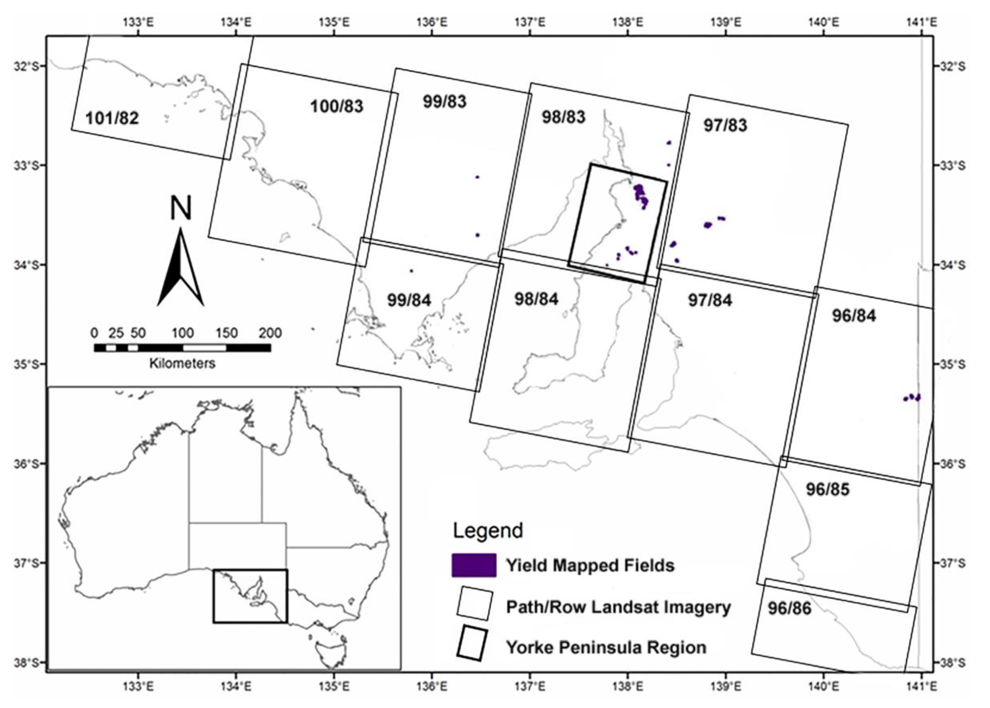
Figure 1. Location and distribution of yield-mapped fields (purple points) and the spatial distribution of Landsat images (path/row) for the Yorke Peninsula region (within Landsat image 98/83) and the state of South Australia. Inset is South Australia in relation to the Australian continent.
Ijgi 12 00050 g001
Figure 2. Wheat and barley yield vs. NDVI scatter graphs and fitted empirical power models for the eight years in the YPA and the two global models (Global* excludes the 2001 wheat yield and NDVI data).
Ijgi 12 00050 g002
Figure 3. Wheat and barley yield vs. NDVI scatter graphs and fitted empirical power models for the state-wide analysis for 2004, 2005 and 2006.
Ijgi 12 00050 g003
Figure 4. Predicted high-resolution yield estimates from yield–NDVI relationships for the state-wide analysis for 2004 and 2005 to 2006. Insets show the fine resolution at which yield is estimated, highlighting yield patterns within a field across the state-wide study area.
Ijgi 12 00050 g004
Figure 5. (A) Scatter plot of regional yields predicted from yield–NDVI models versus yields reported at the administrative region level for 2004, 2005 and 2006. (B) Scatter plot of yields predicted from Landsat NDVI images from 2004, 2005 and 2006 from the yield–NDVI relationship developed in 2005 versus reported yields at the administrative region level. Each data point represents predicted versus reported yield for one administrative region. (C) Nash–Sutcliffe efficiency criterion (E) for annual, interannual and all-years yield prediction models.
Ijgi 12 00050 g005
Table 1. Overall accuracy and Kappa statistic for the YPA and state-wide regions by year. State-wide classifications include the earliest and latest image dates for the 11 classified images.
Day/Month/YearOverall Accuracy (%)Kappa Statistic (%)
6 October 19998070
1 August 20019084
12 September 20034110
11 October 20045017
20 September 2005478
15 September 20065933
2 September 20077460
12 September 20086037
State-wide 25 September–29 October 2004384
State-wide 1 September–4 October 20054316
State-wide 1 September–21 September 2006365
Table 2. Power empirical relationships, R2 and efficiency criteria (root mean square error (RMSE), % of RMSE of average yield and the Nash–Sutcliffe Efficiency Criterion (E)) for the annual wheat and barley and global yield prediction models within the YPA.
YearCropTraining Set (n)Empirical RelationshipR2Validation Set (n)Root Mean Square Error (RMSE) (t/ha)% RMSE of Average YieldNash–Sutcliffe Efficiency Criterion (E)
1999Wheat2137y = 2.33x0.430.139160.42290.12
1999Barley2137y = 3.39x0.330.359160.30140.39
1999Pooled4274y = 1.80x0.050.00218280.5330−0.02
2001Wheat2300y = 5.97x0.310.099820.53110.11
2001Barley2300y = 6.87x0.920.229820.65150.26
2001Pooled4600y = 4.46x0.0080.0019640.7216−0.01
2003Wheat4000y = 4.25x0.870.4340000.91310.14
2003Barley4000y = 4.59x0.520.2440000.77210.18
2003Pooled8000y = 4.59x0.780.3480000.91270.14
2004Wheat800y = 3.82x0.800.238000.48260.18
2004Barley800y = 3.84x0.570.098000.48200.08
2004Pooled1600y = 4.92x0.980.2916000.51240.25
2005Wheat3900y = 6.22x1.330.5638850.55230.59
2005Barley3900y = 5.39x0.720.4938850.59190.47
2005Pooled7800y = 5.47x0.950.3877700.79320.40
2006Wheat5000y = 3.24x0.960.1950000.54320.14
2006Barley5000y = 3.21x0.960.1250000.71440.08
2006Pooled10,000y = 3.24x0.970.1610,0000.63380.11
2007Wheat5000y = 4.81x1.420.5650000.47200.49
2007Barley5000y = 5.03x1.400.2250000.73280.16
2007Pooled10,000y = 4.99x1.440.3910,0000.62250.31
2008Wheat3000y = 9.14x2.090.4530000.80300.27
2008Barley3000y = 3.66x0.330.00330000.80260.002
2008Pooled6000y = 6.11x1.300.2260000.86300.08
GlobalWheat6400y = 4.70x0.990.3264001.10460.19
GlobalBarley6400y = 4.12x0.560.2064000.95320.26
GlobalPooled12,800y = 4.28x0.740.2412,8001.12390.22
Global excluding 2001 wheatWheat5600y = 4.10x0.940.4356000.67320.41
Global excluding 2001 wheatPooled12,000y = 4.08x0.740.2812,0000.93360.29
Table 3. Power empirical relationships, R2 and efficiency criteria (root mean square error (RMSE), % of RMSE of average yield and the Nash–Sutcliffe Efficiency Criterion (E)) for the annual wheat and barley and the 2005 model for the state-wide analysis in 2004, 2005 and 2006.
YearCropEmpirical RelationshipR2Root Mean Square Error (RMSE) (t/ha)% RMSE of Average YieldNash–Sutcliffe Efficiency Criterion (E)
2004Wheaty = 2.26x0.330.110.54300.11
2004Barleyy = 4.00x0.740.480.67280.33
2005Wheaty = 4.58x1.780.490.73300.27
2005Barleyy = 5.73x1.480.530.78260.49
2006Wheaty = 5.43x2.620.600.52400.43
2006Barleyy = 3.55x1.550.150.64500.08
2004Pooledy = 3.01x0.550.250.69330.20
2005Pooledy = 5.49x1.800.450.76260.40
2006Pooledy = 4.21x1.970.360.85660.22
2005 on 2004Wheatas aboveas above0.8547−1.19
2005 on 2004 Barleyas aboveas above0.8539−0.26
2005 on 2006 Wheatas aboveas above0.60460.26
2005 on 2006 Barleyas aboveas above1.1892−2.19
2005 model on 2004 dataPooledas aboveas above1.0148−0.72
2005 model on 2006 dataPooledas aboveas above0.7256−0.15
Disclaimer/Publisher’s Note: The statements, opinions and data contained in all publications are solely those of the individual author(s) and contributor(s) and not of MDPI and/or the editor(s). MDPI and/or the editor(s) disclaim responsibility for any injury to people or property resulting from any ideas, methods, instructions or products referred to in the content.