General Data Search Algorithms for Earth Simulation Systems with Cyclic Boundaries

Abstract

Grid remapping is one of the most fundamental functions in Earth simulation systems, and is essentially a kind of data interpolation. The key to an efficient interpolation method is how to quickly find the relevant grid points required for interpolation. With the rise of unstructured grid models, the demand for general and efficient interpolation search algorithms is becoming stronger and stronger. KD (K-dimensional) tree has proven to be effective in dealing with unstructured grids. However, it is unable to tackle the cyclic boundary conditions in Earth simulation systems, which restricts the application of KD tree. Taking the nearest neighbor search as an example, this paper introduces two new KD tree-based multi-dimensional data search methods, which break through the limitations of the original method with regards to the cyclic boundary. One method is based on target points duplication, and the other method is based on source points duplication. Their time complexity and space complexity are analyzed and verified by carefully designed experiments. The results show that the method based on target points duplication generally performs better than that based on source points duplication when the data are basically evenly distributed.

1. Introduction

The Earth simulation system [1] has developed from a single model (e.g., atmospheric model, ocean model) to a coupled system (e.g., ocean–atmosphere coupled system), and is of significant importance in the prediction of climate change and early warning of natural disasters. For coupled systems, grid remapping technology is a vital bridge for data interaction between component models.

In essence, grid remapping is a kind of data interpolation. In terms of conservation, interpolation methods can be divided into conservative interpolation and non-conservative interpolation. Conservative interpolation [2] needs to consider the grid area and even the earth curvature to ensure the conservation of flux (e.g., momentum flux, heat flux), while non-conservative interpolation usually only considers the location of grid points. For non-conservative interpolation, the data value on the target grid is actually the weighted average of the data value on the source grid. For example, inverse distance weight interpolation [3] uses the reciprocal of distance from the source point to the target point as the weight of each source point. Other traditional non-conservative interpolation methods include nearest neighbor interpolation [4], bilinear interpolation [5], etc. However, no matter which interpolation method is used, the core problem is establishing the relevant source points, and whether or not the relevant points can be discovered quickly directly has a direct effect on the efficiency of interpolation.

A great number of methods have been developed for data searches in multi-dimensional space [6,7,8]. However, most of these methods cannot deal with disordered data, which means they can hardly tackle unstructured grid problems. With the rise of unstructured grid models (e.g., FVCOM), the demand for general interpolation search algorithms is becoming stronger and stronger. At present, the mainstream interpolation tools (e.g., SCRIP [9]) adopt the blocking method for data search, that is, the search space is divided into several blocks, and the target grid uses violent search in the blocks. However, the efficiency and correctness of this method largely depend on the setting of the block size and the distribution of data. If the block is too large, the violent search would take a long time, while if the block is too small, the correct point may not be found. Therefore, a more general and robust data search algorithm is required.

Implementing a general data search based on KD tree, which was firstly proposed by Bentley [10], is a potential choice. KD tree can be treated as a special binary tree. The distinction between a KD tree and an ordinary binary tree is that an ordinary binary tree always divides its data by a constant dimension, while a KD tree can be divided by any dimension in each layer according to requirements. The dimension with the largest variance or the widest dispersion is usually selected to be split, so as to divide the search space as evenly as possible. The median point is usually selected as the partition point, so as to build a balanced KD tree which would reduce the tree height and shorten the search time [11]. After the completion of KD tree construction, the whole search space is organized in the form of a binary tree according to the division order. A data search based on KD tree consists of two steps. The first step is to compare the value on the specified partition dimension with the selected partition point from the top level to the bottom level, until the leaf node is found. This means that the target point is located in the sub-space represented by the leaf node. The second step is to trace back layer by layer, and judge whether another sub-tree may have related points. Once such possibility exists, the other sub-tree would be searched immediately in the same way. Therefore, the data search based on KD tree is usually implemented by recursive algorithm.

A great deal of effort has been made to improve the efficiency of data research based on KD tree. In order to find the median point faster during the construction process, Brown [12] proposed a method based on presorted results, which solved the problem of the quick select method being subject to data arrangement. Cao et al. [13,14] further improved its efficiency by introducing additional data structures. The sampling technique could be adopted to estimate the median point [15], which makes it suitable for large-scale data sets. Besides, parallel technology is widely used in the construction and data search of KD tree [16,17,18]. From the perspective of parallel granularity, the mainstream parallel schemes can be divided into two categories. One is data level parallelism, and the other is task level parallelism. There will be data interaction between cores in data level parallelism (e.g., parallel partition point selection), while the data in each core will be relatively independent in task level parallelism (e.g., parallel sub-tree construction).

KD tree has been widely used in multi-dimensional vital data search, especially in nearest neighbor search and range search. Hou et al. [19] used KD tree to improve the efficiency of data classification, which is a vital field in data mining. Another improvement in KD tree was made by Havran et al. [20] in the field of ray tracing. Guo [21] applied KD tree in point cloud registration field. He et al. [22] proposed a new cloud data indexing method based on KD tree. In order to deal with large deformation problems in computational fluid dynamics (CFD) field, a new interpolation method for unstructured mesh based on KD tree had been implemented by Guo et al. [23]. Guo et al. [24] also developed a KD tree-based method to find the nearest distance from a flow point to the wall in CFD field. Cao et al. [25] have even tested the potential of KD tree in grid remapping in Earth simulation systems, and the results showed that it can always achieve a reasonable performance regardless of the grid type.

At present, there are few studies in the literature regarding the application of KD tree in grid remapping in Earth simulation systems. One possible reason is that the original KD tree cannot deal with the cyclic boundary. KD tree uses hyperplanes to divide the search space, and the premise of obtaining independent, unique and non-overlapping sub-spaces is that any dimension of the space is acyclic. However, many cases in coupled Earth simulation systems have to deal with grid remapping with cyclic boundaries, such as global simulation (the longitude of the global grid is cyclic) and some regional ideal experiment with cyclic boundaries. Once there are cyclic boundaries in the search space, many conclusions from the original data search process will no longer be tenable. Therefore, it is essential to develop new search algorithms to solve these problems according to the characteristics of cyclic boundaries.

Taking the nearest neighbor search as an example, according to the characteristics of cyclic boundaries, this paper proposes two new search methods capable of handling cyclic boundary problems based on KD tree, which largely expands the current application scope of KD tree. One method is based on target points duplication, and the other method is based on source points duplication. To the best of the authors’ knowledge, this is the first time that KD tree has been utilized to perform a data search in cyclic space. In addition, the time complexity and the space complexity of these two methods are analyzed, and some general suggestions are given according to their performance in the experiments.

The rest of the sections in this paper are organized as follows: detailed description and complexity analysis of these two new methods are given in Section 2, experiments analysis and verification are shown in Section 3, and the conclusion is drawn in Section 4.

2. Algorithm

2.1. Basic Idea

When considering the cyclic space, an artificial boundary is usually proposed to divide the continuous space, which is called cyclic boundary or circular boundary. In this way, two virtual finite boundaries appear in the cyclic dimension, and all the data are located in a specified loop segment. Referring to the method of setting halo points around local boundaries in order to realize the communication between adjacent points in the process of parallel computing, this paper proposes similar mirror methods to fulfill the vital data search in multi-dimensional cyclic space based on KD tree.

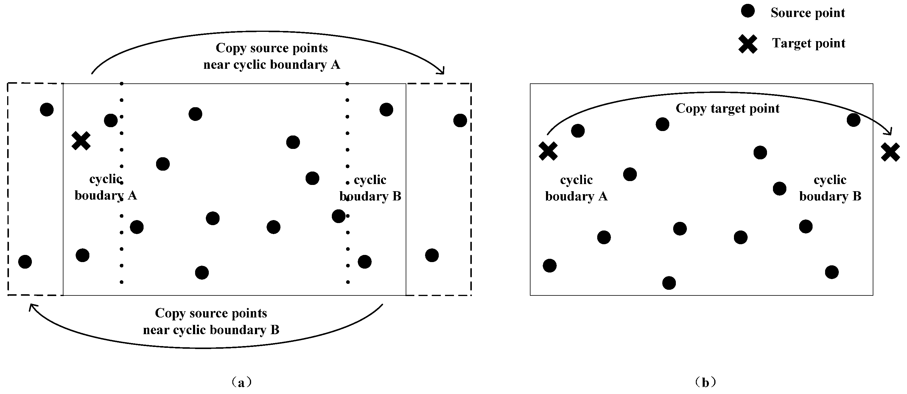
Taking the nearest neighbor search in 2D space with only one cyclic boundary along the vertical direction as an example (see Figure 1), the mirror method has two basic schemes based on the selection of replicated objects. The first scheme is to duplicate related source points as mirror points, that is, copying source points near cyclic boundary A to the right side of cyclic boundary B, and copying source points near cyclic boundary B to the left side of cyclic boundary A. The maximum area for each replication is half of the entire search space (see Figure 1a). The cost of this scheme is that more storage space is required to store those mirror points. At the same time, as the scale of source data increases, the construction time of KD tree will also increase. In addition, the search time will also increase to a certain extent due to the deepened tree. If the distribution of the source data has some characteristics that can be further used, such as the maximum distance between any position in the search space and its closest source point, the number of duplicated points can be further controlled. The second scheme is to select the target point for replication. After a complete search with the original method, the target point would be copied to the outside of the cyclic boundary which is located further from the target point (assuming it is cyclic boundary B), then a new round of similar search for the duplicated point would be carried out (see Figure 1b). The final nearest neighbor point is picked up from these two search results. Although this method only requires marginally more storage overhead, the search time is almost doubled. If further optimization of the search process is required to reduce the search time, we should introduce new mechanisms for further pruning during the search process, with the utilization of the characteristics of KD tree and the distribution characteristics of source data and target data. For example, before the replication of the target point, if the distance from the target point to its closest cyclic boundary (assuming it is cyclic boundary A) is greater than the first search result, the replication operation and the second search can be cancelled, because there would not be any closer source points near the other cyclic boundary at this time. Moreover, taking the first search result as the initial nearest distance of the second search can also avoid searching many unnecessary branches in the second search.

2.2. Detailed Description

In this section, we will describe the process of these two methods in detail. It is assumed that the search space has K dimensions with C cyclic boundaries. Without loss of generality, we set D[1] to D[c] as cyclic dimensions, where D[i] represents the i-th dimension.

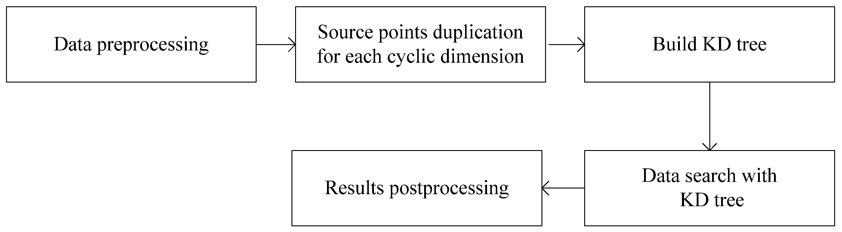
The process of the mirror method based on source points duplication is shown in Figure 2. The first step is to perform data preprocessing, that is, placing all the source points and the target points within a specified loop segment for each cyclic dimension. Subsequently, the source points near one cyclic boundary are copied to the outside of another corresponding cyclic boundary for each cyclic dimension. The scope of the duplication can be determined by the distribution characteristics of source data. For example, if the maximum distance between any position in the search space and its closest source point is L, only the source points within the range of L from the cyclic boundary need to be copied. In fact, the precondition can be further weakened. As long as the source point density near the cyclic boundary reaches such condition, the limited duplication method still works. However, if the distribution characteristics of the source data are unknown or unsure, the maximum duplication area for each cyclic boundary would be half of the original search space. It should be noted that all the duplications should be based on the original location of the source data. After copying the relevant source points for each cyclic dimension, the KD tree can be constructed and the nearest point can be found according to the classical algorithm (more details about these classical algorithms can be seen in [25]). The final step is to map the search results back to the original region or the original point number, similar to the data preprocessing.

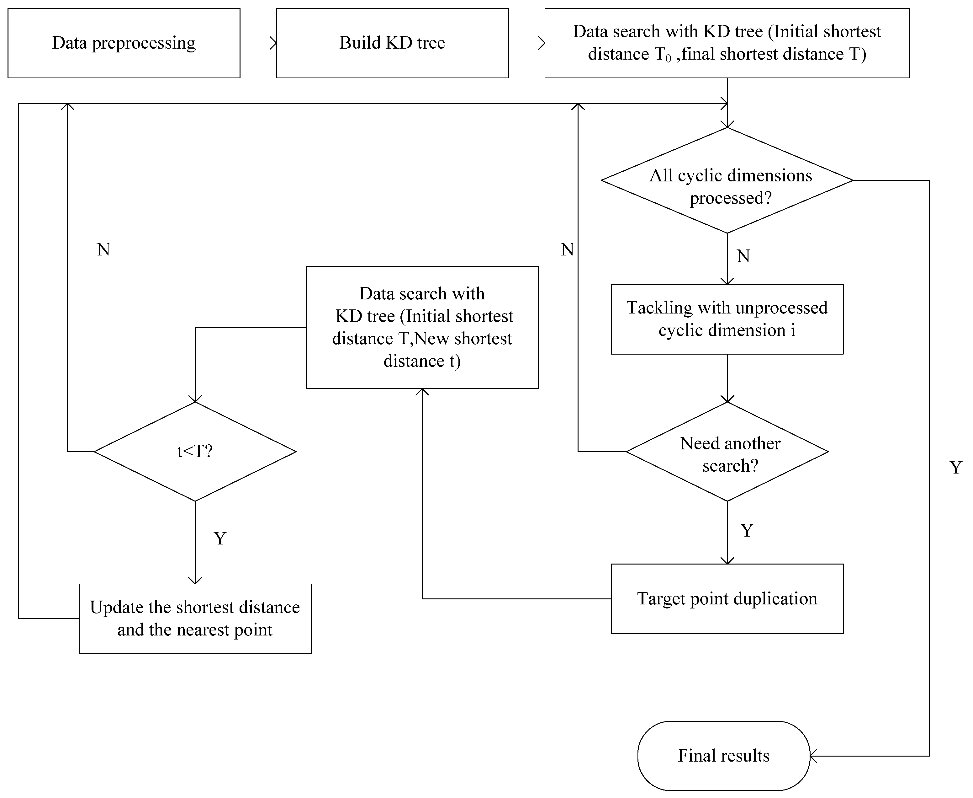
The process of the mirror method based on target points duplication is shown in Figure 3. Initial works, including data preprocessing, KD tree construction, and general nearest point search, are the same as the normal nearest neighbor search based on KD tree. The initial shortest distance T₀ is usually set to a negative number or a sufficiently large value. After the first round of data search, the final shortest distance between the target point and its closest source point is obtained as T. Subsequently, we must approach each cyclic dimension by a special method. For the sake of simplicity, these cyclic dimensions could be processed in turn. When tackling the unprocessed cyclic dimension i, a comparison between the distance from the target point to its nearest cyclic boundary in the i-th dimension S and current shortest distance T should be done at the beginning. If S is not less than T, it means that source points near another cyclic boundary in the i-th dimension cannot be closer than current point. Thus, there is no need to search again for the other cyclic boundary, and we can now start to process the next cyclic dimension. Otherwise, you would need a further search in current cyclic dimension. Before starting a new search, we need to copy the target point to the same relative position outside the corresponding cyclic boundary. The following search could adopt the current shortest distance T as the initial shortest distance value, as it may help us cut off more unnecessary branches in the new search. Assuming that the new nearest distance is t, we should make a comparison between t and T, and select the smallest result as the latest result. It is worth mentioning that if the final nearest distance and the final nearest point use the pass by address mechanism in programming, the update operation can be omitted. After all the cyclic dimensions have undergone the operations described above, the shortest distance and the corresponding source point obtained would be the final result.

2.3. Complexity Analysis

To facilitate the analysis, we assume that the number of the source points is N, and the number of the target points is M. Then, the space complexity of the original KD tree-based search method would be O (N + M), and the average time complexity of KD construction and data search of the original method is O (Nlog₂N) and O (Mlog₂N), respectively. In addition, for convenience of description in the following analysis, we use SPD and TPD to represent the source points duplication method and the target points duplication method, and use CP and SP to represent the construction process and the search process, respectively.

As for the mirror method based on source points duplication, in the worst case, all source points need to be copied for each cyclic space. Under such condition, the space complexity would be O (N + CN + M). The time consumed for KD tree construction would be:

T_SPD,CP = O ((C + 1)Nlog₂ ((C + 1)N))

(1)

The average time consumed for data search would be:

T_SPD,SP = O (Mlog₂((C + 1)N))

(2)

As for the mirror method based on target points duplication, the extra storage overhead for the replicated target point is negligible. Therefore, the space complexity could be written as O (N + M), which is the same as traditional nearest neighbor search based on KD tree. The time consumed for KD tree construction remains the same, which can be written as:

T_TPD,CP = O (Nlog₂N)

(3)

The average time complexity of the data search process has been changed, which could be written as:

T_TPD,SP = O ((βC + 1)Mlog₂N)

(4)

where β is the average replication ratio and varies between 0 and 1. In the worst case, each target point has to undergo a new search in each cyclic dimension, which means β is 1. Under such conditions, the time complexity of the data search process would be O ((CM + M) log₂N). However, in most practical problems, only a small portion of target points near the cyclic boundary need to be searched twice or multiple times (i.e., β tends to 0). Therefore, the search time consumed in practice is usually much lower than the worst estimate. It is worth mentioning that if replication judgment is not adopted, the time complexity of this method will be the worst result.

Comparing these two mirror methods, it can be found that the space complexity and the time complexity of the construction process based on target points duplication is always much better than that based on source points duplication. Considering the time complexity of the data search process, the performance of the method based on target points duplication relies heavily on the average duplication ratio. If the performance of the mirror method based on target points duplication tends to be worse than that based on source points duplication, it must at least satisfy:

T_TPD,SP-T_SPD,SP = (βC + 1)Mlog₂N-Mlog₂((C + 1)N) > 0

(5)

After simplification, it can be written as:

β > β_threshold = log₂(C + 1)/(Clog₂N), C > 0

(6)

It can be seen from Equation (6) that β_threshold decreases with the increase of N and C. In practice, the overhead of the search process for duplicated target points will be less than that of a traditional search, because the new search already has a reliable shortest distance at the beginning, which will greatly reduce the unnecessary search branches during the backtracking process. It means that, in general, only when β is much greater than the threshold value computed above, would the mirror method based on target points duplication perform worse than that based on source points duplication.

3. Experiments

These two mirror methods are implemented in C language in our experiments. The split dimension is selected in natural order, and the quick select method [26,27] is used to find the median data during the construction of KD tree. The first element is always chosen as the pivot element in our quick select method for the sake of simplicity. More details about the basic process of KD tree construction and data search based on the KD tree can be seen in [25]. Two basic data sets, with 2²⁴ randomly generated 6-dimensional real data in each, are used in the following experiments. Each element in the 6-dimensional data has a value between 0 and 100 with 6 valid decimal places. In the following experiments, random data set 1 is used as the source data and random data set 2 is used as the target data. Since the distribution characteristics of the source data are uncertain for randomly generated data, all the source points are copied for each cyclic dimension in the mirror method based on source points duplication. The correctness of these two methods is verified by cross validation using the same data, and relevant results for correctness verification are not shown in this paper.

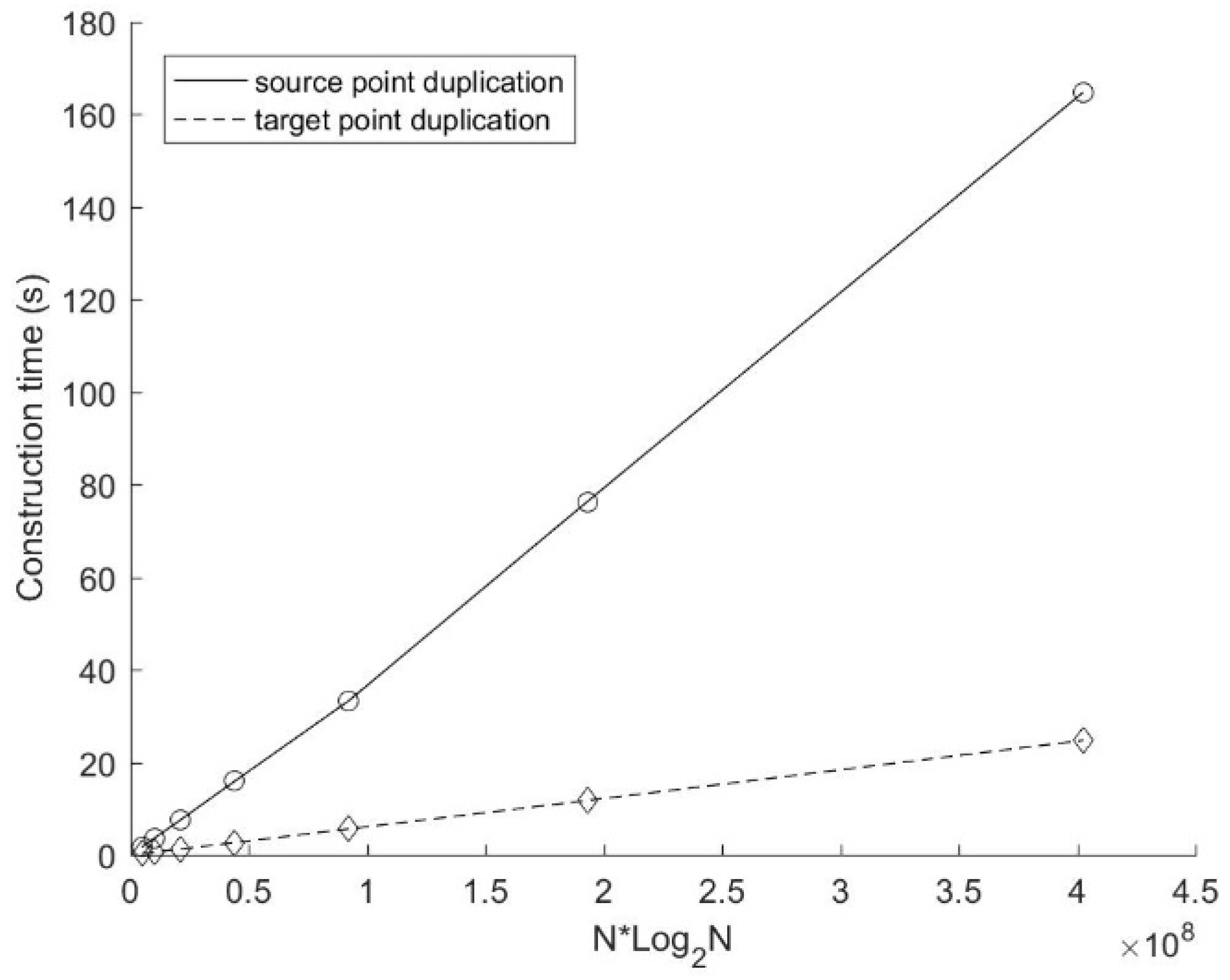
Figure 4 and Figure 5 show the construction time and the search time of these two mirror methods with different number of source points respectively. In this experiment, K = 4 (i.e., both source and target points are 4D data). The number of target points M is 2²¹ and the number of cyclic dimensions C is 4. The number of source points N varies from 2¹⁸ to 2²⁴, which is doubled each time. As can be seen from Figure 4, the construction time of the mirror method based on target points duplication is proportional to Nlog₂N, which is consistent with the time complexity we analyzed above (Equation (3)). 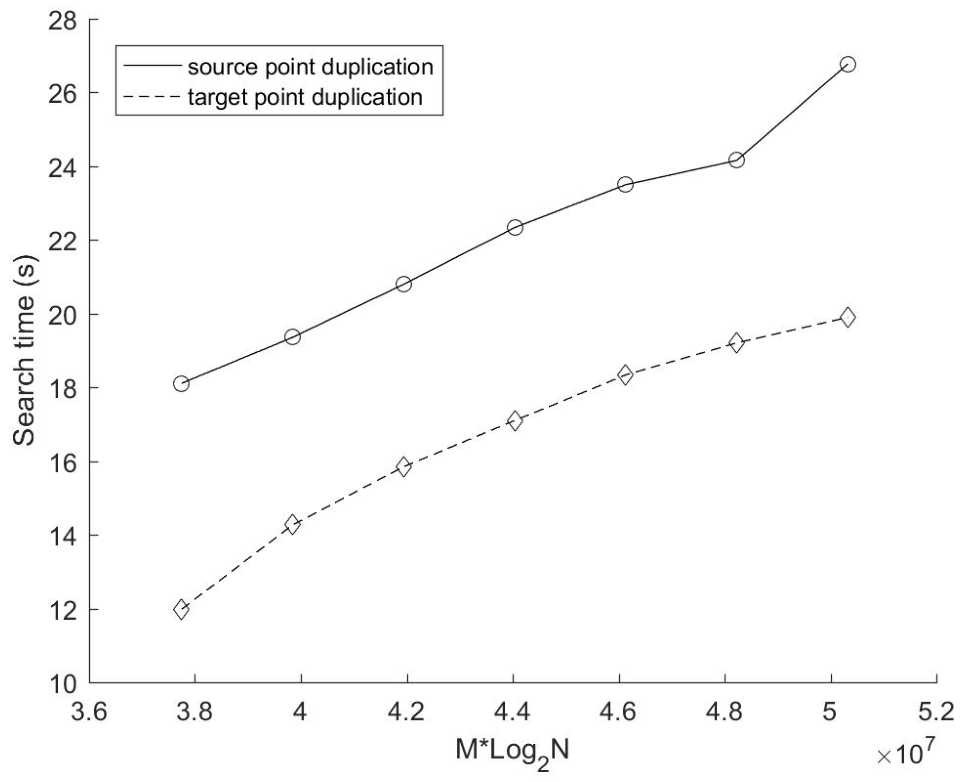While the construction time of the mirror method based on source points duplication is much higher (more than five times than that based on target points duplication), this is in line with our analysis of its time complexity (O (5Nlog₂5N) according to Equation (1)). In terms of the performance of the data search, Figure 5 shows that the mirror method based on target points duplication is still better than that based on source points duplication under the current configuration. The growth of the search time of the mirror method based on source points duplication is almost proportional to Mlog₂N. According to the search time complexity of the source points duplication method deduced above (Equation (2), its derivative to Mlog₂N satisfies:

$$\frac{\partial {\mathrm{Mlog}}_2\left(\left(\mathrm{C}+1\right)\mathrm{N}\right)}{\partial {\mathrm{Mlog}}_2\mathrm{N}}\propto \frac{\partial {\log }_2\left(\left(\mathrm{C}+1\right)\mathrm{N}\right)}{\partial \mathrm{N}}\frac{\partial \mathrm{N}}{\partial {\log }_2\mathrm{N}}\propto 1=\mathrm{constant}$$

(7)

The formula deduced above demonstrates that the growth trend of the search time of the source points duplication method depicted in Figure 5 is reasonable. In addition, it can be seen clearly that the growth rate of the search time of the target points duplication method decreases significantly with the increase of source points number. This is because the augment of source points would generally reduce the number of target points duplication.

Figure 6 further reveals the variation of the actual average replication ratio β and the threshold of average replication ratio β_threshold with different number of source points in this experiment. The solid line demonstrates that only a small portion of points (less than 6% on average for each cyclic dimension) are duplicated during the search, which shows the importance of the replication judgment strategy proposed in the target points duplication method. In terms of growth trends, it can be seen clearly from the picture that β and β_threshold are both decreasing with the augment of source points. The decline rate of the actual average replication ratio is closely related to the number and the distribution of source points and target points. In this experiment, the decline rate of β is larger than that of β_threshold. Moreover, β is greater than β_threshold when N < 2²². According to previous analysis, the search time of the method based on target points duplication may be larger than that based on source points duplication. However, this phenomenon does not occur (see Figure 5). This is because the copied target point has already owned an appropriate nearest distance before a new data search, which reduces the number of branches that need to be accessed during the backtracking process, resulting in a less time consumption for copied target points than a conventional search. In this experiment, β is only a little higher than β_threshold, and the extra overhead in theory is compensated by the excellent performance of those copied target points in practice. Therefore, there is no case that the search time of the mirror method based on target points duplication is greater than that based on source points duplication in current experiment.

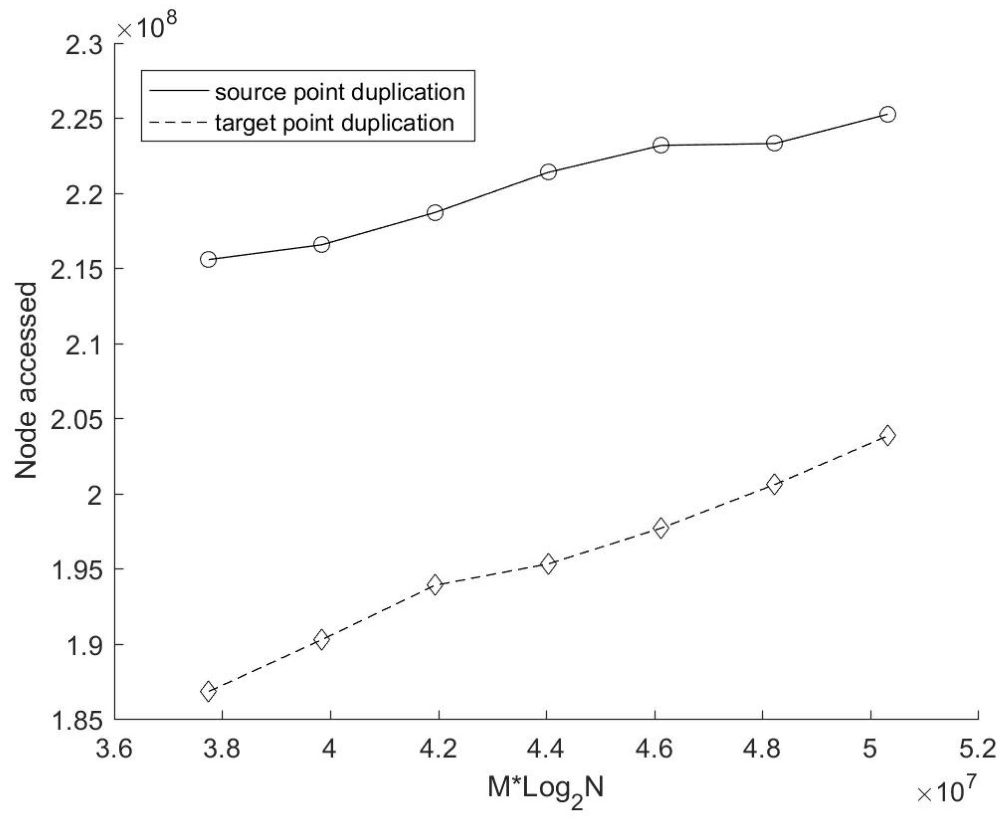
In order to further verify our inference, we counted the number of nodes accessed in the search process (i.e., the number of times to calculate the distance) of these two methods (see Figure 7), because this is the most time-consuming part of the whole search process. As can be seen from the figure, the number of nodes accessed in the source points duplication method is always higher than that in the target points duplication method, which is also the direct reason why the search time based on source points duplication is always higher than that based on target points duplication.

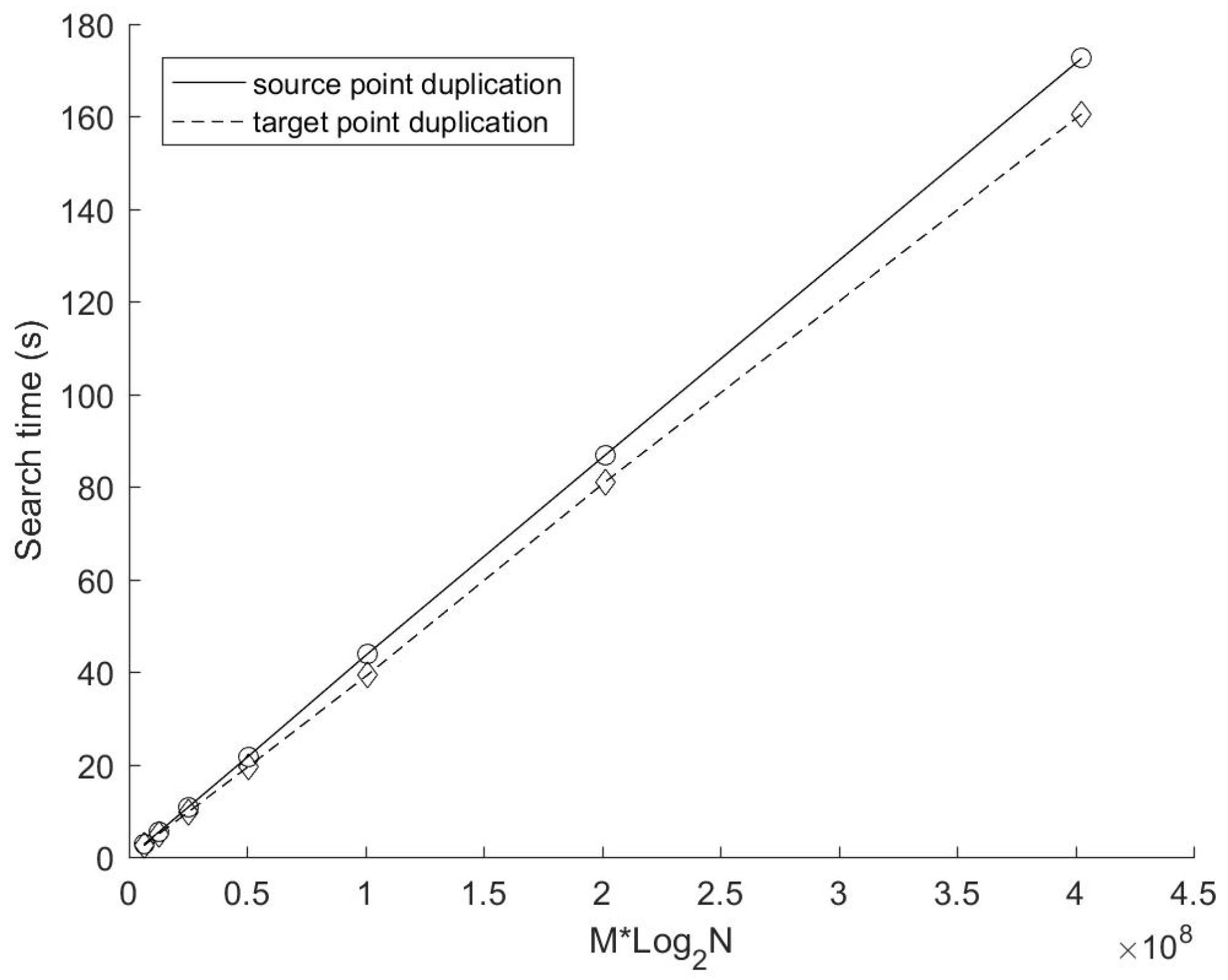
Figure 8 shows the search time of these two methods with a different number of target points. In this experiment, the number of data dimensions and the number of cyclic dimensions is the same as those in the previous experiment (i.e., K = 4, C = 4). The number of source points N is fixed at 2²⁴, while the number of target points M varies from 2¹⁸ to 2²⁴ (doubled each time). Obviously, the search time of both methods increases linearly with the number of target points. In addition, the search time of the target points duplication method still performs better than that of the source points duplication method. 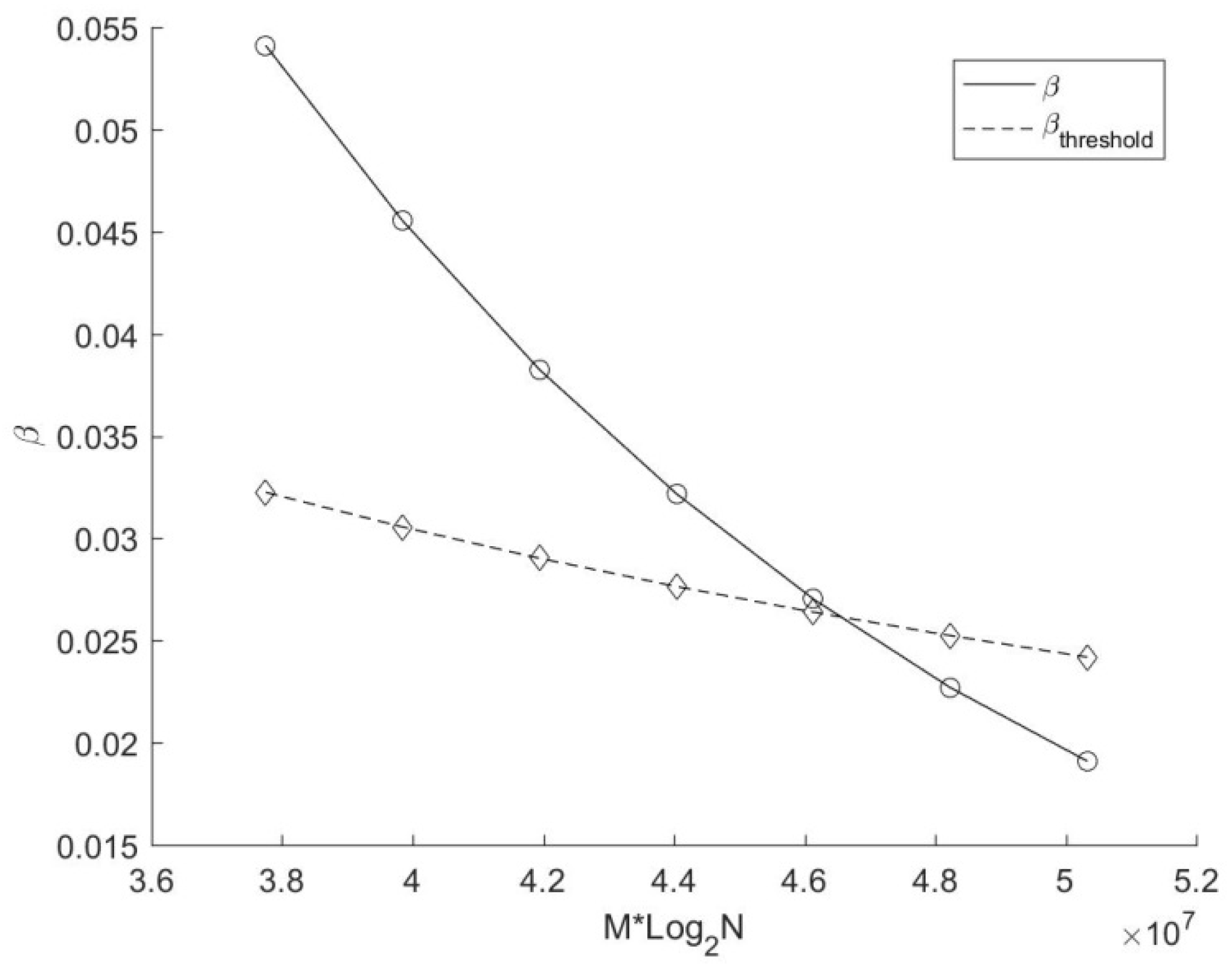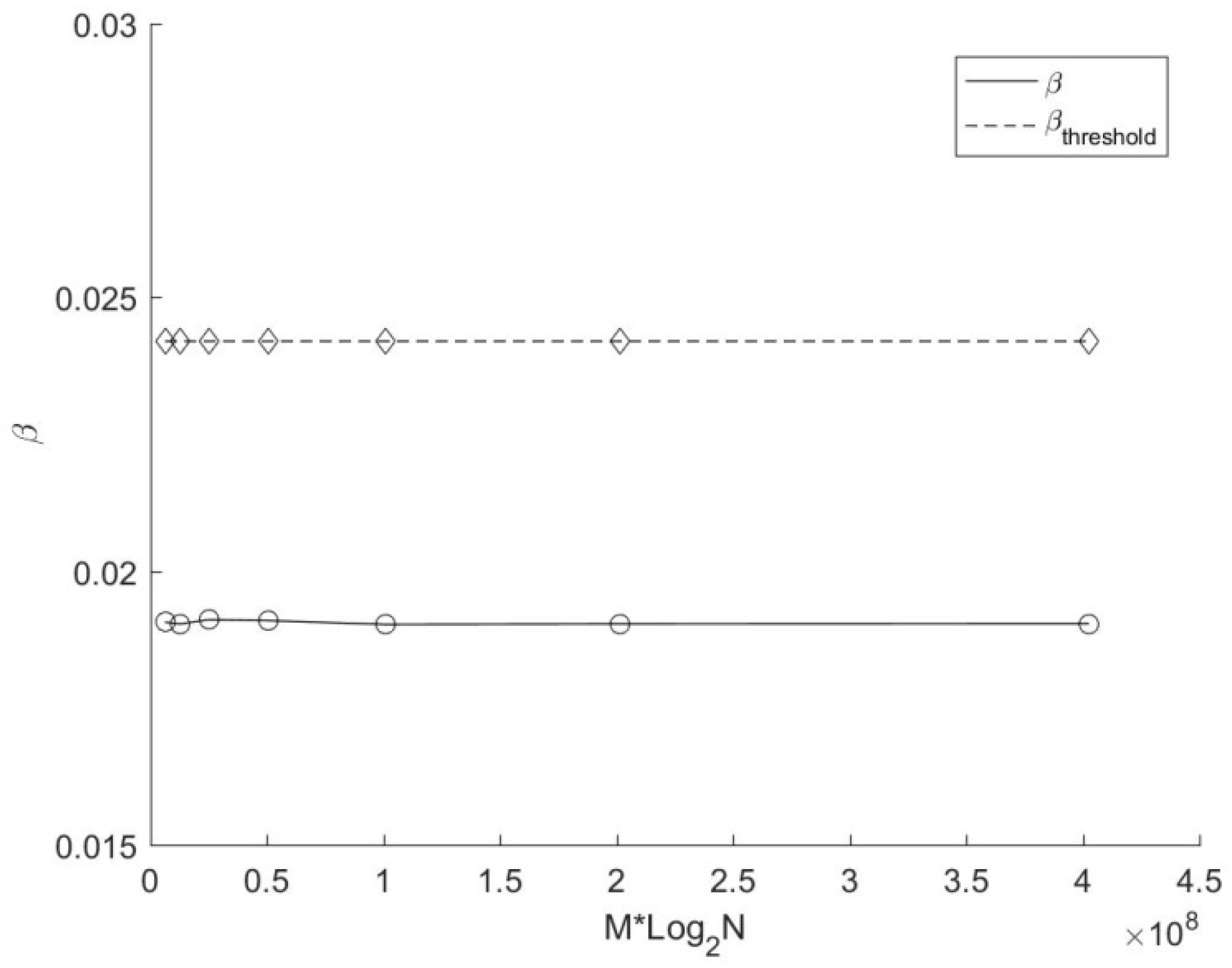Figure 9 depicts the variation of β and β_threshold with a different number of target points in this experiment. As can be seen from the picture, β_threshold is a constant, and is always greater than β. Therefore, it makes sense that the search time of the target points duplication method is less than that of the source points duplication method in this experiment. Moreover, although the actual average replication ratio β fluctuated slightly, it remained stable on the whole. In other words, for data sets with randomly generated elements, the variation of M will not lead to a significant change in β as long as M is large enough.

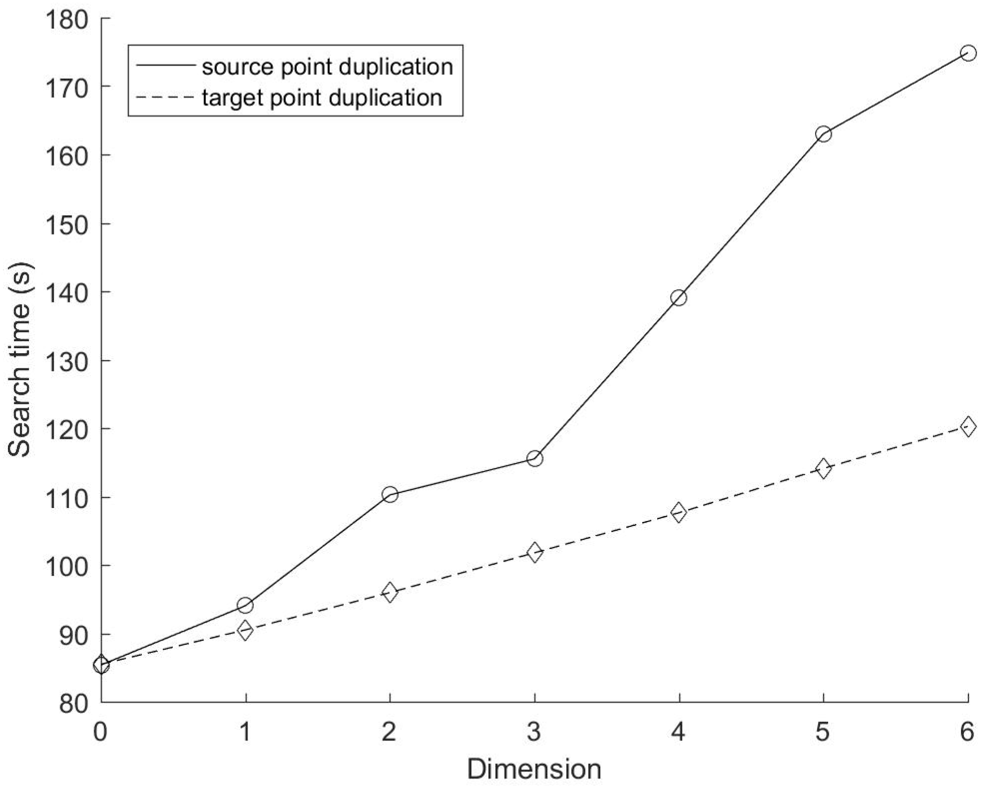
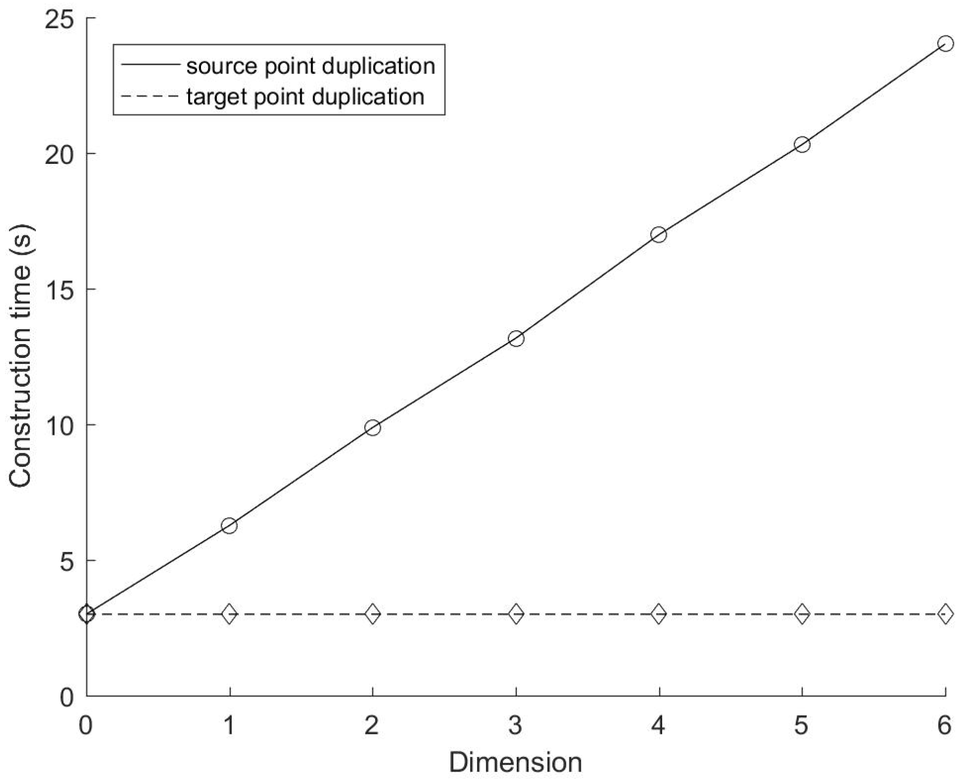
Figure 10 and Figure 11 show the time consumption of KD tree construction and data search of these two methods with different number of cyclic dimensions, respectively. In this experiment, K = 6, N = M = 2²¹, C varies from 0 to 6, increasing by 1 each time. For the mirror method based on target points duplication, the KD tree construction time does not change with the variation of the number of cyclic dimensions. However, the construction time of the mirror method based on source points duplication increases slightly higher than the linear growth rate. According to the previous analysis on the construction time complexity of the source points duplication method (Equation (1)), its derivative to the cyclic dimension is:

$$\frac{\partial \left(\mathrm{C}+1\right){\mathrm{Nlog}}_2\left(\left(\mathrm{C}+1\right)\mathrm{N}\right)}{\partial \mathrm{C}}={\mathrm{Nlog}}_2\left(\left(\mathrm{C}+1\right)\mathrm{N}\right)+\mathrm{N}/\ln 2$$

(8)

The first term on the right side of Equation (8) increases slowly with the increase of C, while the second term is a constant. Therefore, the trend of the construction time of the source points duplication method is reasonable. Figure 11 shows that the search time of the target points duplication method is basically linear with the number of cyclic dimensions. This is because the derivative of the search time of the target points duplication method (Equation (4)) to the cyclic dimension is:

$$\frac{\partial \left(\mathsf{\beta }\mathrm{C}+1\right){\mathrm{Mlog}}_2\mathrm{N}}{\partial \mathrm{C}}\propto \frac{\partial \mathsf{\beta }}{\partial \mathrm{C}}\mathrm{C}+\mathsf{\beta }$$

(9)

In this experiment, the number of source points and target points remain unchanged, and all these points are evenly distributed, and the range of each dimension is the same, so the actual target point replication ratio is almost the same for each dimension, which means β can be regarded as a constant. Therefore, it is reasonable that the search time of the target points duplication method increases linearly with the number of cyclic dimensions in this experiment. The search time of the source points duplication method changes irregularly with the cyclic dimension, and is always higher (except C = 0) than that of the target points duplication method.

4. Conclusions

This paper developed two new cyclic space data search algorithms based on KD tree, which solved the cyclic boundary problem in Earth simulation systems. Taking the nearest neighbor search as an example, this paper analyzed the spatial and temporal complexity of KD tree construction and data search of these two methods, and verified their performance through experiments. The results showed that the mirror method based on target points duplication performs much better than that based on source points duplication in terms of memory overhead and construction speed. As for the consumption of data search, the mirror method based on target points duplication usually also performed better under the condition that the source points and the target points were evenly distributed. Moreover, it should be noted that, though current methods only searched for the nearest point, they could be easily applied for K nearest points search and range search with minor modifications.

In addition, it is particularly worth reiterating that, as the proposed methods were general data search algorithms for multi-dimensional cyclic space, they could be used not only in grid remapping in Earth simulation systems, but also in other systems with cyclic space data search problems (especially for unstructured grid or disordered data), such as observation thinning in data assimilation systems and data search in geographic information systems. Future research may focus on the effective utilization of these methods in different application fields.