Adaptive Spatio-Temporal Query Strategies in Blockchain

Abstract

In various applications of blockchain, how to index spatio-temporal data more efficiently has become a subject of continuous attention. The existing spatio-temporal data query in the blockchain is realized by adding additional external storage or fixed spatio-temporal index in the block, without considering the distribution of the spatio-temporal query itself and the proof performance accompanying the query. We propose an adaptive spatio-temporal blockchain index method, called Verkle AR*-tree, which adds the verification of time and location in the blockchain without additional storage and realizes the spatio-temporal index with an encrypted signature. Verkle AR*-tree further provides an adaptive algorithm, which adjusts the tree structure according to the historical query to produce the optimized index structure. The experimental results based on the pokeman dataset show that compared with the existing static spatio-temporal index, our method can effectively increase the performance of the spatio-temporal query and the spatio-temporal commitment in the blockchain.

1. Introduction

Blockchain is a rapidly advancing distributed ledger technology [1] that has expanded from originally decentralized financial transactions to more real-world applications [2] including merchandise trade, supply chain services, resource allocation services, goods transportation, IoT, etc. These application scenarios have brought new challenges to the original blockchain technology. Blockchain needs not only to complete decentralized transaction security verification, but also effectively construct distributed data storage to achieve optimal data query performance. For example, in trade transactions the blockchain is responsible for ensuring that “the transactions of company A are true” in the decentralized environment, now it also needs to ensure that “the transactions of company A in Shanghai port on 3 January 2022 are true”, and further facilitate the retrieval of “all transactions completed by company A in Shanghai port in January”.

Many advances have been made in the research of blockchain integrated with spatio-temporal data. The sidechains [3] are provided on the blockchain dominated by bitcoin [4], in which the time information is stored in the mainchain while the spatial information is stored in the sidechain, and the mutual locking of space-time information is realized through SPV(Simplified Payment Verification Proof) two-way peg [5]. In Ethereum [6,7], the ethernet db realizes the parser from block storage to a relational database, making the traditional spatio-temporal query technology applicable to blockchain. In the blockchain based on Block-DAG (BlockChain-Direct Acyclic Graph) [8], a cryptographically signed tree [9] is introduced, in which a Merkle KD tree is implemented, and the blockchain head has a spatial index with trade information.

At present, the difficulties of spatio-temporal blockchain technology focus on increasing the performance of spatio-temporal data queries without increasing the key capabilities cost of its autonomy, audibility and immutability. Therefore, large-scale transformation of data structures or introduction of external databases in blockchain should be avoided as far as possible. In addition, the efficiency of the spatio-temporal index in the blockchain is always related to the spatial distribution of the spatio-temporal query, while the traditional spatio-temporal index is determined by the spatio-temporal data itself, ignoring the statistical distribution of spatio-temporal query, which makes the spatio-temporal index lack of adaptability. To address this situation we propose Verkle AR*-Tree, which integrates the temporal-spatial index with the blockchain Verkle tree [10], and realizes the adaptive index reconfiguration oriented to spatio-temporal query distribution. Based on Verkle AR*-Tree, we have realized the storage of three types of spatio-temporal information in the blockchain, including transactions with time and location, account information with last location and spatio-temporal trajectory of the account. We accelerate spatio-temporal region query through adaptive indexing, and improve the proof efficiency of data through vector commitment of Verkle. The experimental results show that our method can effectively embed the spatio-temporal data into the blockchain, and the query efficiency is better than the existing static spatio-temporal index blockchain.

The rest of this paper is organized as follows: the related research is summarized in Section 2 and the details about the construction of the Verkle AR*-tree are in Section 3. The evaluation is presented in Section 4. Section 5 is the discuss and Section 6 concludes this work.

2. Related Work

2.1. Spatio-Temporal Index

Spatio-temporal indexes divide a given spatio-temporal region hierarchically and place spatio-temporal objects in a divided node. According to the different ways of spatial object organization, spatial index methods are generally divided into object mapping, object bounding, clipping and multiple layers [11]. We simply divide the spatio-temporal indexes into two categories: regularization and irregularization, The former has no overlapping spatio-temporal regions of nodes in the same layer, and the partition always runs through a subregion, such as quadtree tree [12], KD tree [13] and BD tree [14], and the latter such as BSP tree[15], MLS3 [16], R tree [17,18,19]. R-tree is actually a spatio-temporal index family. As a balanced tree supporting high-dimensional spatial data, R-tree is widely used in spatio-temporal data management. R-tree is a dynamic spatio-temporal index data structure. The insertion, deletion and query of nodes can be parallel. Spatial objects are stored in leaf nodes with minimum boundary rectangles, and the spatial regions represented by each node can overlap. Too much overlap sometimes affects the performance of data query, so variants such as R+ tree[18], cell tree [20] allow an object to belong to multiple leaf nodes to avoid too much backtracking in tree nodes search. Another improvement is to optimize the utilization of node space and the balance of the R-tree. For example, Hilbert R-tree [21] uses a Hilbert fractal curve to sort k-dimensional data in one dimension. R*-Tree [19] believes that the overlap of node space areas can be improved by forcing node insertion and reducing the number of node splitting.

After 40 years of research, spatio-temporal index has developed a wealth of algorithms and data structures. As a mature field, the recent interest focuses on the application of various industries. However, almost all algorithms rely only on spatio-temporal objects rather than the distribution of queries. As shown in Figure 1, (A) is the splitting result of five two-dimensional spatial objects (a, b, c, d, e) in the R-tree algorithm, where (a, c, d) belong to the child node A, and (b, e) belong to child node B. (B) shows the splitting result of R*-tree algorithm, from which it can be seen that R*-tree has a smaller node overlap area, but smaller node overlap does not mean higher query performance. As shown in (C), for the frequently occurring query window W, both R-tree and R*-tree need to access two nodes, although only object b will become the query result. The spatio-temporal index still needs to be extended to have query adaptability.

2.2. Blockchain

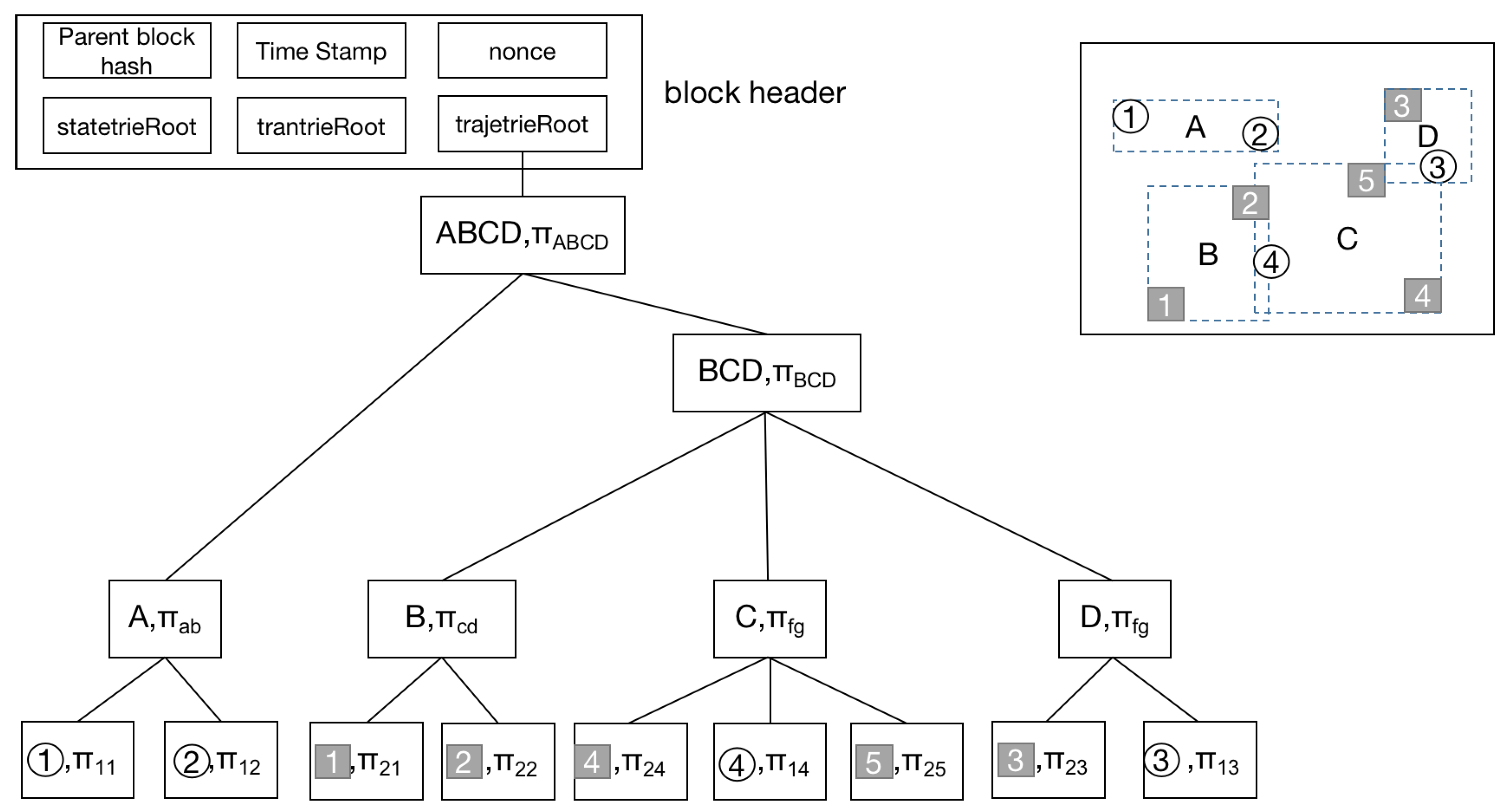
2.2.1. Architecture of Blockchain

A blockchain is a decentralized, and trustless ledger technology that provides reliable transactions. Security, decentralization and scalability cannot be combined [22]. In the balance of the three, blockchain technology has undergone three generations of evolution.

The first generation of blockchain 1.0 architecture represented by Bitcoin is a single chain composed of blocks, in which each block contains a head and a body of several transactions’ information. The key data structures in the block are shown in Figure 2. The block header contains the version information of the block, the root node of Merkle tree, the hash value and timestamp of the parent block, etc. the block body stores encrypted transaction records and the hash value of encrypted information, but does not store detailed account information. In the blockchain 2.0 architecture represented by Ethereum, Merkle Tree is improved to Merkle Patricia Tree (MPT) [23]. MPT supports both trade management and account storage. It combines the advantages of Merkle Trees and Patricia Trees, where Patricia Trees are an index for prefix trees, and can query and update faster and cost less computing resources. A scalable Block-DAG protocol named Phantom is proposed in [24], which is the main architecture of blockchain 3.0. Block-DAG can greatly improve the transaction efficiency of the blockchain, by allowing each block to have more than one parent block to support parallel processing.

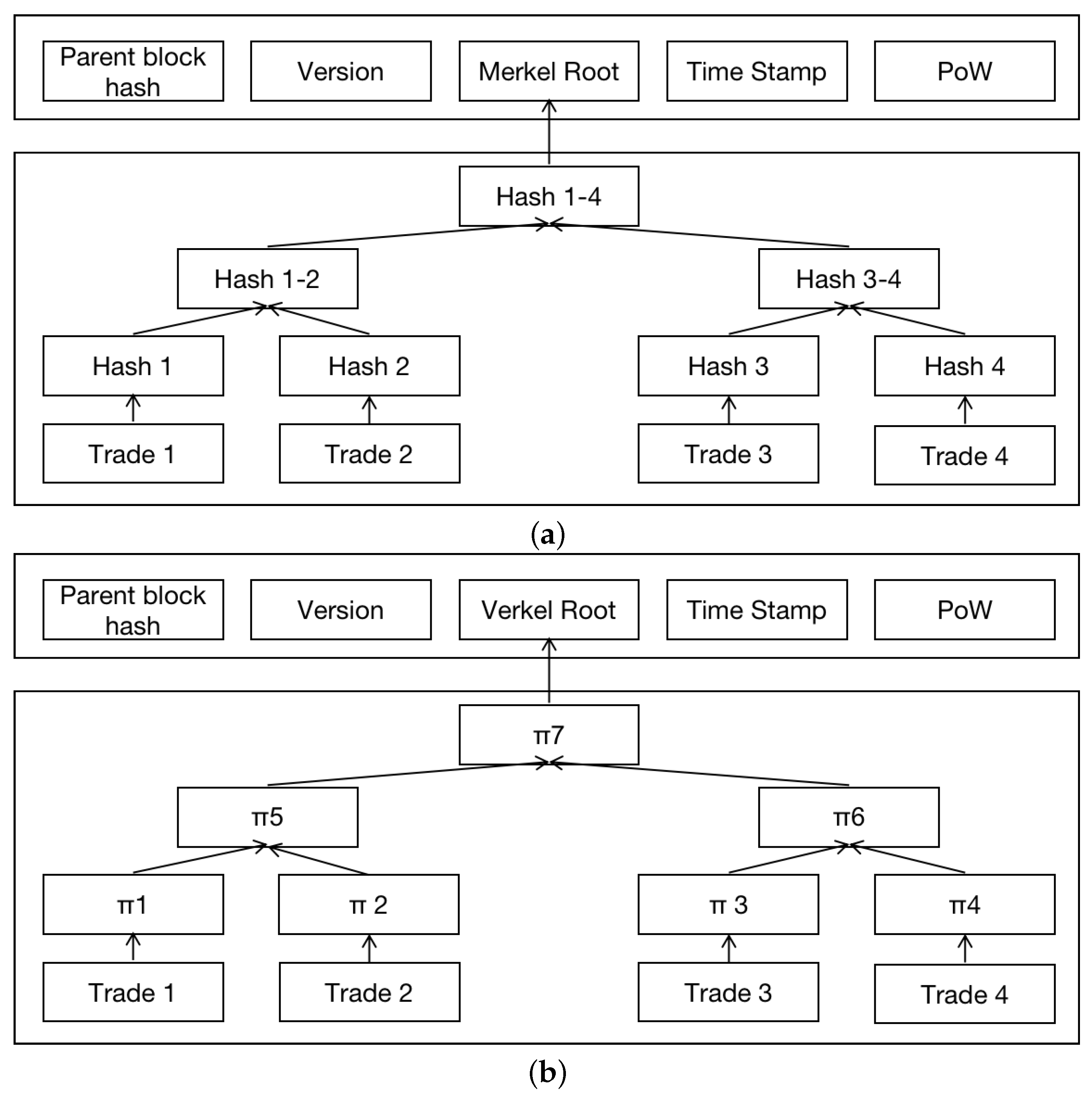
2.2.2. Merkle Trees and Verkle Trees

A Merkle Tree [25] is a binary balanced tree based on the hash value, which can be an efficient digital signature framework and ensure that data from each block is not corrupted in distributed networks. The security of a Merkle tree-based digital signature scheme only depends on the security of the hash function and does not need too many theoretical assumptions, which makes the Merkle tree-based digital signature more secure and practical. In the Merkle tree, the hash value of each transaction is stored in the leaf node. The combined hash of two adjacent leaf nodes is taken as the new hash value from bottom to top, the resulting Merkle root needs to be saved in the block header. The client can quickly verify whether the node belongs to the Merkle tree through the value of the node, the value of the Merkle root and the related path, so as to quickly verify whether a transaction is included in the block.

There has also been progressing in proving the authenticity of data in the blockchain. In [10] proposes Verkle trees, a more bandwidth-effective alternative to Merkle trees. In the latter, the parent node is the hash of its children, while in the former, the parent node is the vector commitment of its children. As shown in Figure 2, the Merkle proof for Trade 2 needs to provide the hash (hash 2, hash 1, hash 3–4) of all sibling nodes, which increases with the increase of tree depth and k-args, while the Verkle proof only needs to provide the proof on the path from leaf node to root node (${\pi }_2$, ${\pi }_5$, ${\pi }_7$).

2.2.3. Spatio-Temporal Index in Blockchain

In the continuous upgrading of blockchain architecture, many technologies that integrate spatio-temporal data in blockchain have been proposed [3,7,26,27,28,29]. In our work, we focus on spatio-temporal blockchain technology that integrates spatio-temporal data validation capabilities, which require a transaction data proof structure combined with spatio-temporal indexing. An important aspect of spatio-temporal blockchain is that of spatio-temporal data verification. The known verifiable spatio-temporal index methods include Merkle KD-Tree [9,30] and Merkle R-Tree [31], but the integration of spatial index verification and retrieval technology with adaptive query ability in the latest Verkle tree is still lacking.

Merkle KD-tree [9] have been presented in block-DAG that maintains integrity through cryptographically signed history and maintains the efficient spatio-temporal queries without additional local store. In Merkle KD-tree, a KD-tree for indexing 3D point objects is integrated into the block-DAG, Merkle proof is added to the nodes of the KD-Tree, its digest is put into the block header, and the time label of the transaction is stored independently in the block header. Experiments show that Merkle KD-Tree has better performance in various spatio-temporal queries, such as range queries, KNN queries, etc. The drawback of the Merkle KD tree is that it only applies to point objects, and the temporal information needs to be indexed separately from the spatial information.

Merkle R-Tree [31] is another technology that implements spatio-temporal indexing in the blockchain, where each internal node is associated with a Merkle digest over the MBRs and digests of its children. Its main shortcoming is that the transaction data is stored in the block, while the spatio-temporal R-tree index and Merkle proof are implemented in an outsourced database, which actually reduces the security guarantee of the blockchain.

3. Verkle AR*-Tree in Spatio-Temporal Blockchain

3.1. Preliminary

We present the definitions of related concepts in this section.

Definition 1 (MBR): the minimum bounding rectangle (MBR) of irregular two- dimensional spatial objects is tuple <left, right, top, bottom>.

Definition 2 (TMBR): minimum bounding rectangle with timestamp (TMBR) of spatio-temporal objects is tuple <left, right, top, bottom, begin, end>.

Definition 3 (TWST): transaction with spatio-temporal information (TWST) is tuple <geoId, TMBR, account, event>. A transaction is stored as cryptographically-signed stream.

Definition 4 (AWLP): Account with last position information (AWLP) is tuple <accountId, lastposition, timestamp, data> with a hash key generated by account name.

Definition 5 (Block): Block includes a block header and a block body consisting of the corresponding transaction records. The transaction records are assembled into a tree structure using a membership proofs scheme such as Merkle tree, Verkle tree, etc. In our work, we use a Verkle tree. The block header is tuple <blockID, parenthash, statetrieRoot, trantrieRoot, trajetrieRoot, TMBR, timestamp, nonce>, where parenthash is hash of parent block, statetrieRoot is a digest of account trie, trantrieRoot is a digest of transaction trie, trajectorytrieRoot is a digest of the trajectory of account in a given time frame, timestamp represents the creation time of the block, and nonce is a 64-bit hash that proves the sufficient amount of computation.

Definition 6 (Cost Model): The cost model refers to the average probability that each node will be visited when the query range is given, which is also a function of the depth of the tree and the spatial distribution of nodes at all levels.

Definition 7 (query): We consider three kinds of queries: (1) region query of transactions. Given a window TMBR, we query all transaction information intersected with spatio-temporal TMBR with its related Verkle proof. (2) last location information of account. Given the hash key of an account, find the account data and its last location information. (3) trajectories of account. Given the query window TMBR and the hash key of an account, query the trajectories of the account in the TMBR.

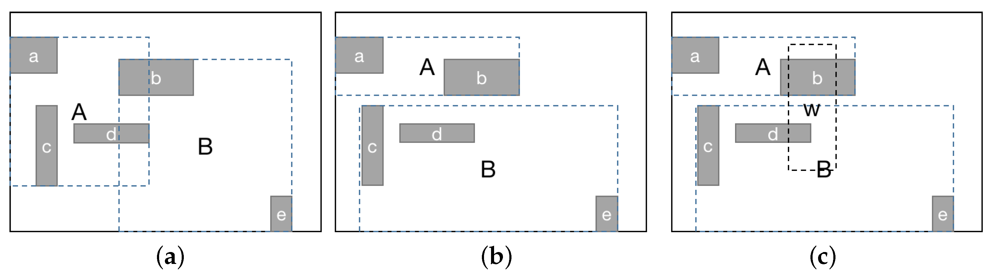
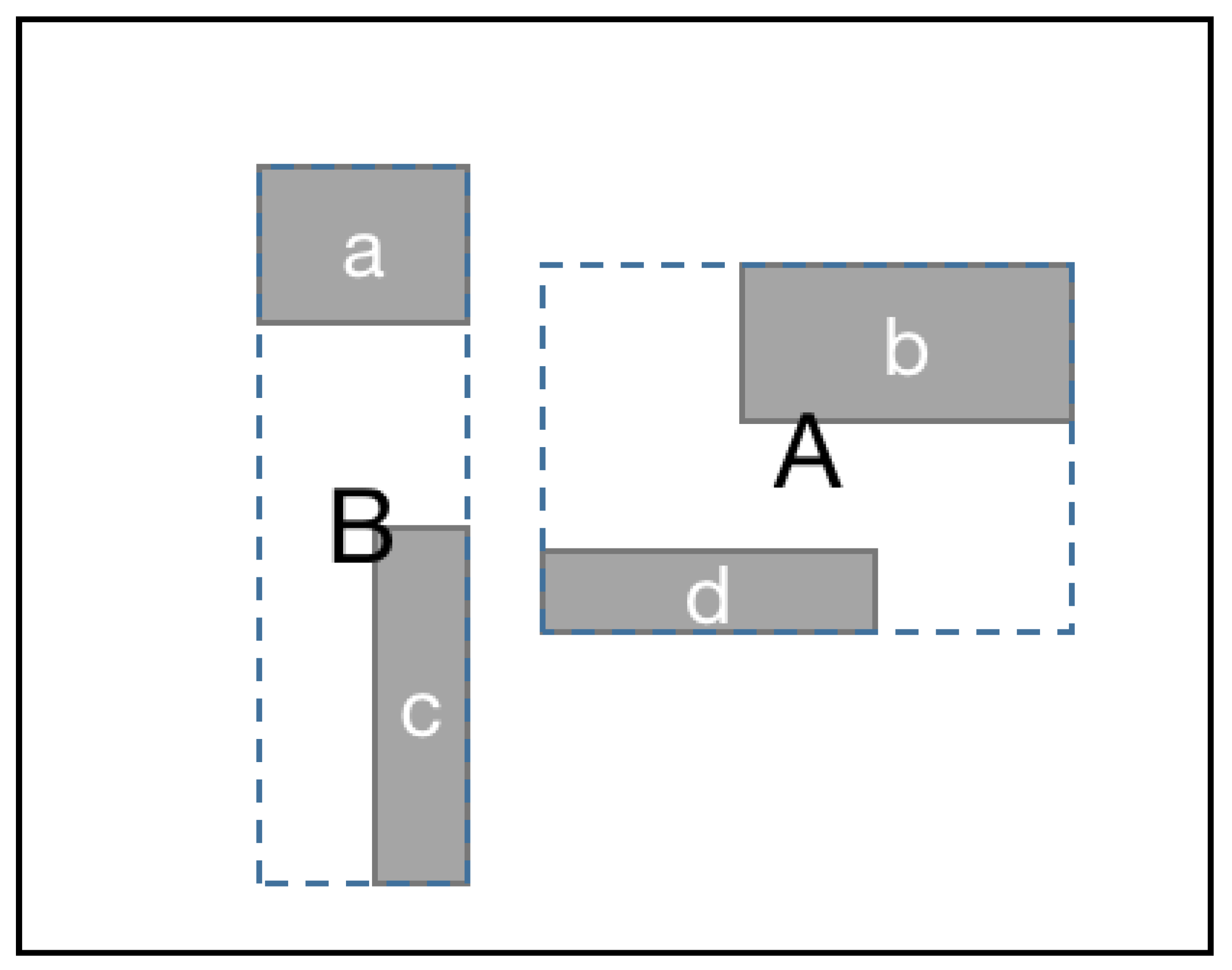
3.2. Verkle AR*-Tree

Three kinds of data are stored in the block body. The account information includes the account name with the last position of the account and relevant data which changes frequently, while the transaction does not change after the block is created. The trajectories of the account only retaining a fixed period in the block to prevent block overflow needs to be queried and deleted regularly. We use different indexing methods for these three kinds of data. For account information, we use the Verkle Patricia Trie (VPT), for the transactions and the trajectories, we use Verkle AR*-Tree.

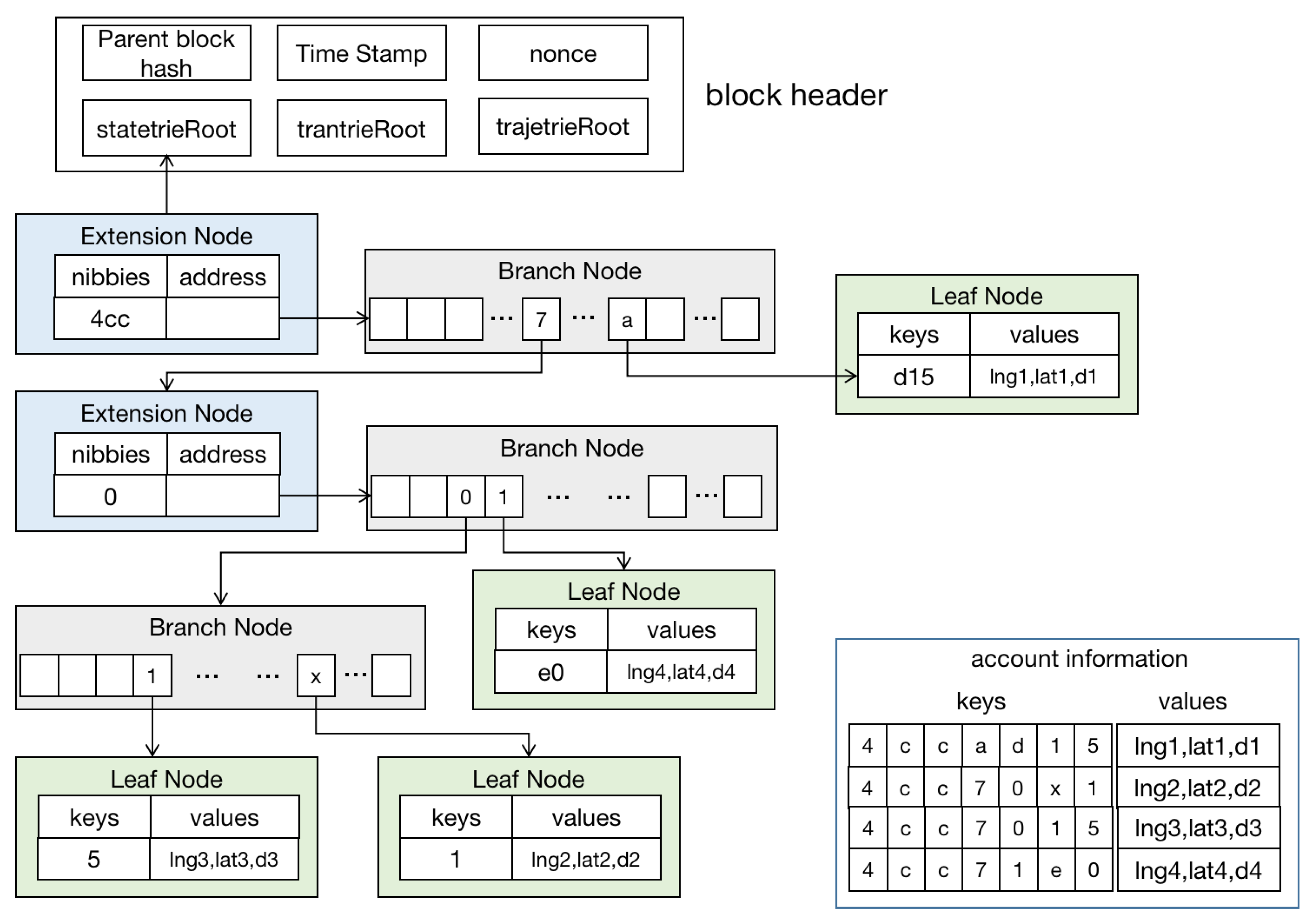
3.2.1. Index of Account with the Last location

The account information is stored in Verkle Patricia trie (VPT) with location data, and the storage structure is shown in Figure 3. Each account consists of the hashed key and value. The VPT tree has three types of nodes. The leaf node stores the account data and the Verkle commitment. The extension node consists of a key and an address pointing to the branch node. The branch node consists of up to 256 addresses and a Verkle commitment, which points to the next extension child node or leaf node, respectively.

Given the hash key of an account, such as “4ccad15”, access the extension node (4cc) from the root node, then find the 97th item (code of ‘a’) of the branch node, and finally access the leaf node (d15), get the encrypted value of the leaf node and the vector commitment values of all nodes on the path together.

Given the updated account information, the update algorithm of VPT (Algorithm 1) is as follows.

Algorithm 1 Update algorithm of VPT.

Input:

vpt: a Verkle patricia trie

node: current node in VPT

acc(keys,values): account information to be updated

Output:

vpt: updated VPT

1:  if node is nil then

2:  node ← createLeafNode(acc)

3:  vpt.root ← node

4:  else

5:  if node.type is LeftNode then

6:    p ← maxLengthPrefix(acc.keys, node.keys)

7:    newe, newb ← createExtensionNode(p), createBranchNode()

8:    newb.children[node.keys[len(p)]] ← node

9:    newb.children[acc.keys(len(p))] ← createLeftNode(acc)

10:    newb.parent, newe.parent ← newe, node.parent

11:  else if node.type is ExtensionNode then

12:    p ← maxLengthPrefix(acc.keys, node.nibbs)

13:    if p == node.nibbs then

14:      acc.keys = acc.keys[len(p):]

15:      Update(vpt,node.next,acc)

16:    else if node.nibbs.startWith(p) then

17:      newe, newb ← createExtensionNode(p), createBranchNode()

18:      newb.children[node.nibbs[len(p)]] getsnode

19:      newb.children[acc.keys(len(p))] ← createLeftNode(acc)

20:      newb.parent, newe.parent ← newe, node.parent

21:    else

22:      newb ← createBranchNode()

23:      newb.parent ← node.parent

24:      newb.children[acc.keys[0]] ← createLeftNode(acc)

25:      newb.children[node.nibbs[0]] ← node

26:      node.nibbs ← node.nibbs[1:]

27:    end if

28:  else if node.type is BranchNode then

29:    if node.children[acc.keys[0]] is nil then

30:      node.children[acc.keys[0]] ← createLeftNode(acc)

31:    else

32:      acc.keys ← acc.keys[1:]

33:      Update(vpt,node.children[acc.keys[0]],acc)

34:    end if

35:  end if

36:  end if

This algorithm inserts account information into the tree as leaf nodes. The algorithm distinguishes four cases. If the current node itself is a leaf node, a new extension node E and branch node B are created, respectively, and E is taken as the parent node of B, and the original leaf node and new leaf node are placed under B. If the current node is an extension node, get the longest public prefix p of the account key and the extension node’s nibbs. There are three possible about p: p is equal to the extension node nibbs, then the child node of the extension node is set as the current node, and the algorithm is recursively called. If p is only part of the extension node nibbs, a new extension node and branch node are created as the parent node of the original extension node. If p is null, a new branch node is created and the account information is put under the branch node. If the current node is a branch node, the algorithm determines whether the sub-item in the branch node corresponding to the account keys is empty. If so, the account information is directly put into the sub-item, otherwise, the sub-item is taken as the current node and executed recursively.

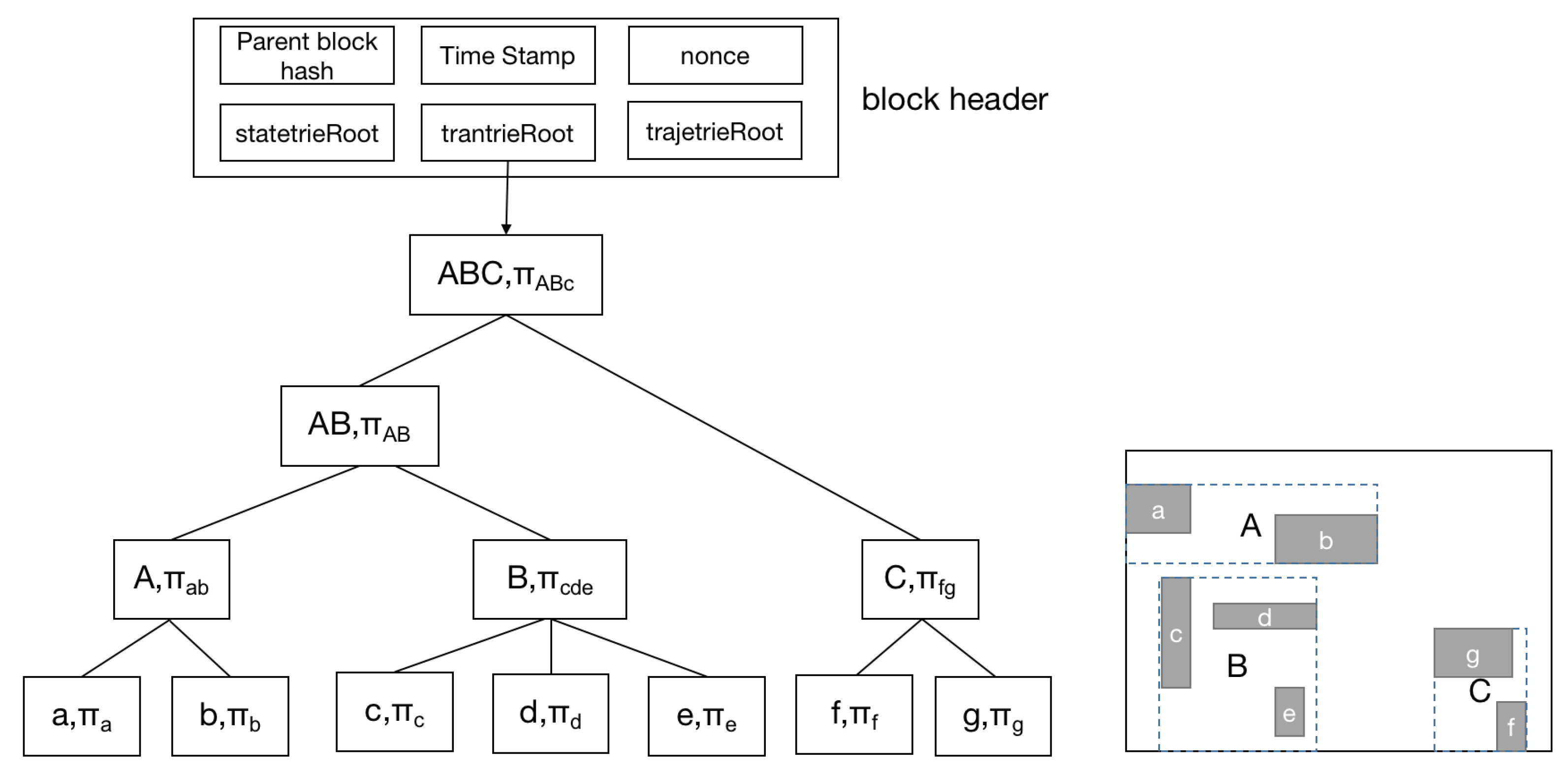
3.2.2. Index of Transaction Information

For transaction information, Verkle AR*-tree is adopted, and the storage structure is shown in Figure 4. The Verkle AR*-tree consists of leaf nodes and middle nodes. Each leaf node contains the hashed transaction information, TMBR, reference count, and vector commitment. The middle node consists of the union of TMBR, reference count, and vector commitment of all its children.

The creation of the Verkle AR*-tree is carried out when the block is created. Each transaction is inserted according to the algorithm in [32]. The only change is that each node needs to compute vector commitment.

Transaction query blockchain is very frequent, so query efficiency is critical to blockchain applications. The R*-tree does not consider the distribution of the query itself. This section further introduces Verkle AR*-tree to increase the adaptive ability. We first propose the query cost model of R*-tree, and then give the adaptive improvement based on the cost model.

Given query window W (wx,wy) and spatial object O (rx,ry), where wx,wy and rx,ry are normalized values of width and height of W and O, respectively, then the probability of the query window intersecting with the object is:

$$Pr=(rx+wx)\ast (ry+wy)/4$$

(1)

Given a full R*-tree with M nodes, if the query distribution is uniform, [33] gives the average number of nodes accessed as follows:

$$Pn=\sum _{i=1}^M(r{x}_i+wx)(r{y}_i+wy)/4$$

(2)

Equation (2) assumes that both data and query are uniform, which is inconsistent with the actual situation. In addition, a query process is carried out layer by layer along the tree nodes, so the average number of nodes visited by a given query window is not simply the sum of each node’s access probability. It is the sum of the product of the intersection probability of each node with the query window and the number of the intersection of the node’s child nodes.

Suppose there is a full R*-tree constructed by N space objects, the number of nodes at the ith layer is $m^{\left(I\right)}$, $1\le I\le H$, where H is the height of the tree and M is the maximum number of child nodes of the node. Given a query window W(wx,wy), the probability of intersection between the spatial rectangle $R_{ij}(rx,ry)$ of any R-tree node and W is denoted as $P{R}_{ij}$, i is the number of the layer, and j is the node number of layer i. Then the average node access number of layer k is:

$$n_k=\sum _{i=1}^{m^{\left(k\right)}}(P{R}_{ki}\times \sum _{j=(i-1)m+1}^{im}P{R}_{k+1,j})$$

(3)

The average number of nodes accessed in the R-tree is the sum of nodes accessed at each layer (the root node is always accessed).

$$\begin{array}{cc}\hfill P_n& =1+\sum _{k=1}^H(\sum _{i=1}^{m^{\left(k\right)}}(P{R}_{ki}\sum _{j=(i-1)M+1}^{iM}P{R}_{(k+1)j}))\hfill \\ \hfill & =1+\sum _{k=1}^H(\sum _{i=1}^{m^{\left(k\right)}}(\frac{1}{4}(r{x}_{ki}+wx)(r{y}_{ki}+wy)\sum _{j=(i-1)M+1}^{iM}(r{x}_{(k+1)j}+wx)(r{k}_{(k+1)j}+wy)/4))\hfill \end{array}$$

(4)

Equation (4) shows that the query efficiency of the R*-tree is closely related to the distribution of sub-nodes. The fewer times the query window intersects a node’s child nodes, the fewer backtrace operations are required. Therefore, the improved idea is to dynamically record the frequency of the query window and adjust the node distribution of the R*-tree according to these frequencies so that the child nodes with frequent queries are merged under the same parent node as far as possible. This can improve the query efficiency of the R*-tree.

We record the query frequency of each node and spatial object. The adaptive optimization of the Verkle AR*-tree includes two aspects: the reconstruction of the Verkle AR*-tree during block creation and the improvement of the splitting algorithm. The reconstruction algorithm (Algorithm 2) is as follows.

Algorithm 2 ReCreate.

Input:

tree: R*-tree

Output:

tree: the reconstructed R*-tree

1:  entries ← tree.allentries()

2:  nodes ← earragenodes(entries)

3:  while True do

4:  results ← rearragenodes(nodes)

5:  parent ← [createNode(children = r) forrinresults]

6:  if parent.length ≤ context.maxchildrennum then

7:    tree.root ← createNode(children = parent)

8:    return

9:  end if

10:  results, nodes ← [], parents

10:  end while

The algorithm starts from all leaf nodes and reconstructs layer by layer, that is, all nodes in each layer are grouped so that the number of nodes in each group is not greater than the threshold. At the same time, the overlapping area between groups is less than the threshold, and the inter-group variance of access frequency is the largest. The grouping algorithm of each layer is implemented as follows (Algorithm 3).

Algorithm 3 Rearragenodes.

Input:

tree: R*-tree

nodes: all nodes of a layer

Output:

groups: node groups

1:  for node ∈ nodes do

2:  for d = 0 to node.dimension do

3:    for j = 0 to 1 do

4:      g1, g2 ← split(nodes, d, node, j)

5:      plans.add(g1,g2)

6:    end for

7:  end for

8:  end for

9:  plans ← sorted(plans, ‘cov’, reversed)

10:  maxcov ← plans[0].cov

11:  plans ← plans[cov == maxcov]

12:  plans ← sorted(plan, ‘overlop’)

13:  return plans[0]

The above algorithm attempts to divide all nodes into two groups at the boundary of each dimension for each MBR. The overlapping area of such groups and the inter-group variance of access frequency are calculated, respectively. All groups shall be sorted in descending order according to the inter-group variance, and the first k (within five of the maximum inter-group variance) shall be reserved. Then, they shall be sorted according to the minimum overlapping area, and the first one shall be taken as the optimal grouping scheme. The process is repeated until the number of nodes in each group is less than the threshold. This algorithm is different from the re-insertion algorithm of R*-tree, in which we rebuild the tree from the bottom up from all the leaves.

The splitting algorithm is similar to the reconstruction algorithm above. All spatio-temporal objects are split according to the edges of all dimensions of all objects. In this way, $2\times N\times D$ splitting schemes can be obtained. N is the number of objects and D is the dimension of spatio-temporal objects. The access frequency, inter-group variance, area and overlap area of each splitting scheme are calculated, respectively. The algorithm first selects the one with a large inter-group variance of access frequency (the difference between the maximum inter-group variance is no more than 5), then selects the one with a small total area (within 20 percent of the minimum total area), and finally selects the splitting scheme with the smallest overlapping area. The improved splitting algorithm is as follows (Algorithm 4).

Algorithm 4 Split.

Input:

entries: entries to be split

Output:

nodes: the split node set

1:  for entry ∈ entries do

2:  for d = 0 to entry.dimension do

3:    for j = 0 to 1 do

4:      g1, g2 ← split(entries, d, entry, j)

5:      plans.add(g1,g2)

6:    end for

7:  end for

8:  end for

9:  plans ← sorted(plans, ‘cov’, reversed)

10:  maxcov ← plans[0].cov

11:  plans ← plans[cov == maxcov]

12:  plans ← sorted(plans, ‘minarea’)

13:  minarea ← plans[0].area

14:  plans ← plans.trim(minarea, 0.)

15:  plans ← sorted(plans, ‘overlop’)

16:  optima ← plans[0]

17:  returnoptima

An example is given to demo the algorithm. As shown in Figure 5, a node has four child nodes, and the algorithm seeks the optimal splitting of this node. Assume that the query frequency of the four sub-nodes is a = 0, b = 4, c = 1, d = 3. There are 16 possible splitting schemes in total. If according to the minimum total area or the minimum overlapping area (R*-tree), C and D should be selected as a group, while according to the access frequency, B and D should be selected as a group.

3.2.3. Index of Trajectory

The index of trajectory is used to query such as “find trajectories of all users in Shanghai port this year”. We still use the Verkle R*-tree (VR), in which the TMBR is four-dimensional and an account dimension is added to TMBR. The value of each account in this dimension is Hamming distance from the account key(16 bits) to “aa...aa”(16-bit). Figure 6 shows a simplified two-dimensional example in which the trajectories of two users are represented as circles and rectangles. The insertion algorithm is the same as algorithm 2, and the function of periodic deletion is added.

4. Experiment

4.1. Experimental Setup

In [9], a KD tree query algorithm and a scan-space algorithm in spatio-temporal blockchain are proposed. We use this algorithm for comparative experiments. We use the same pokeman data set (https://github.com/ILDAR9/spatiotemporal_blockdag, accessed on 1 July 2022), which provides 18,732 records, each of which includes longitude, latitude, time and pokeman type. The spatial data and timestamp data are normalized to (0–1). We are concerned with three properties of our algorithm:

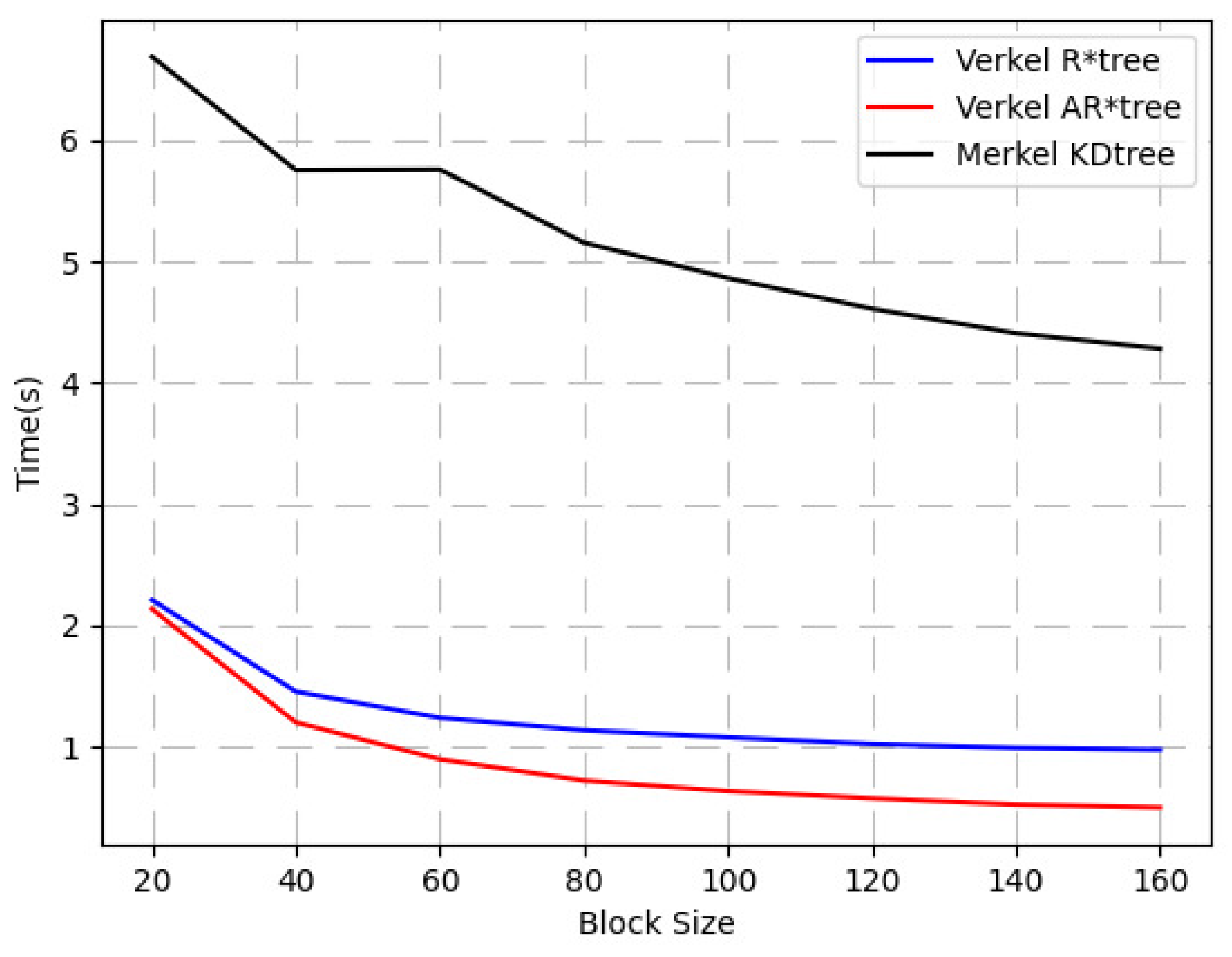
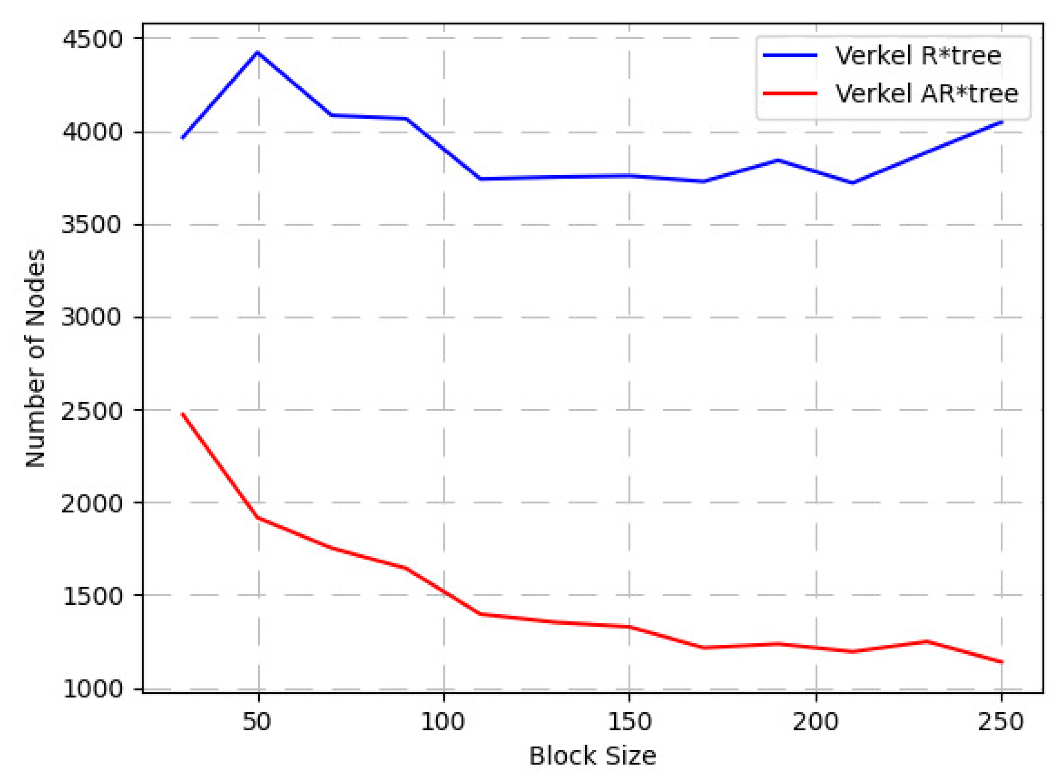
• Whether the spatio-temporal query performance of Verkle AR*-tree proposed in our work is better than the benchmark in [9] which reports that the spatio-temporal query performance is greatly affected by the block size, so we use different block sizes to compare the query performance.
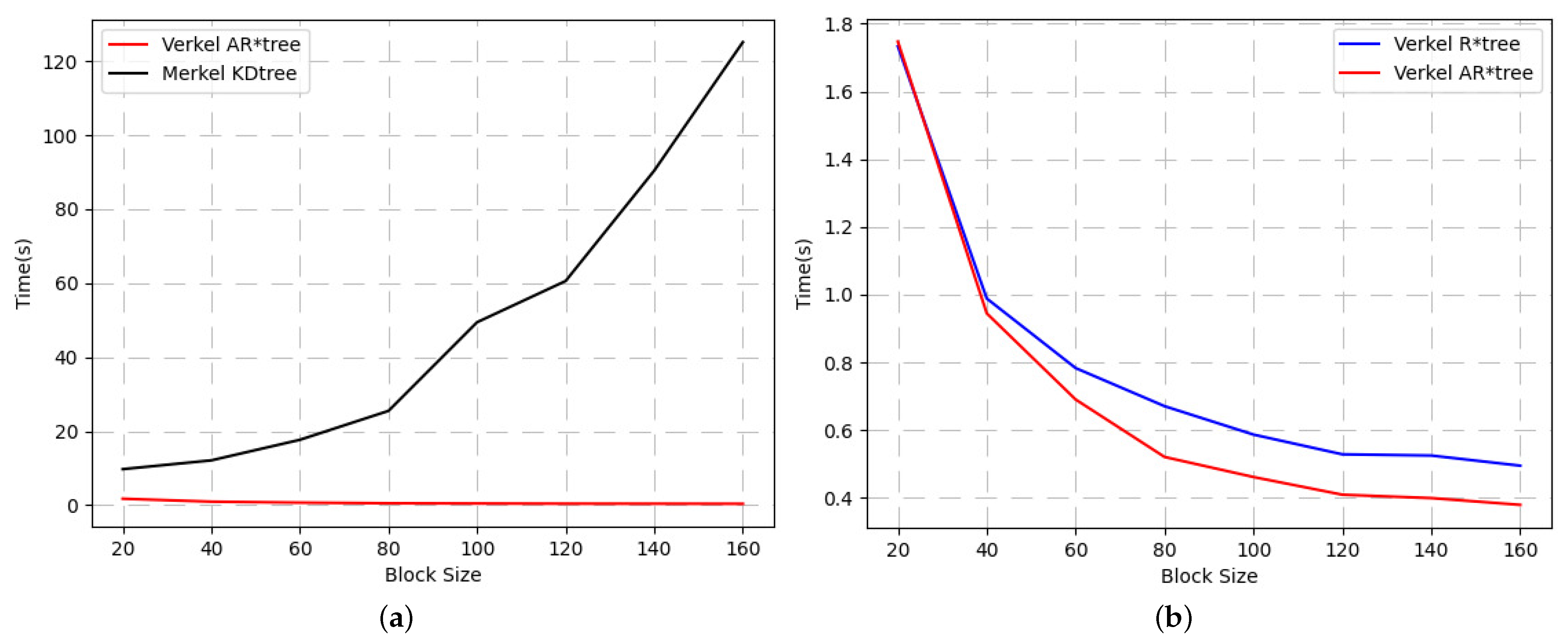
• Performance comparison between adaptive AR*-tree and R*-tree in the blockchain.
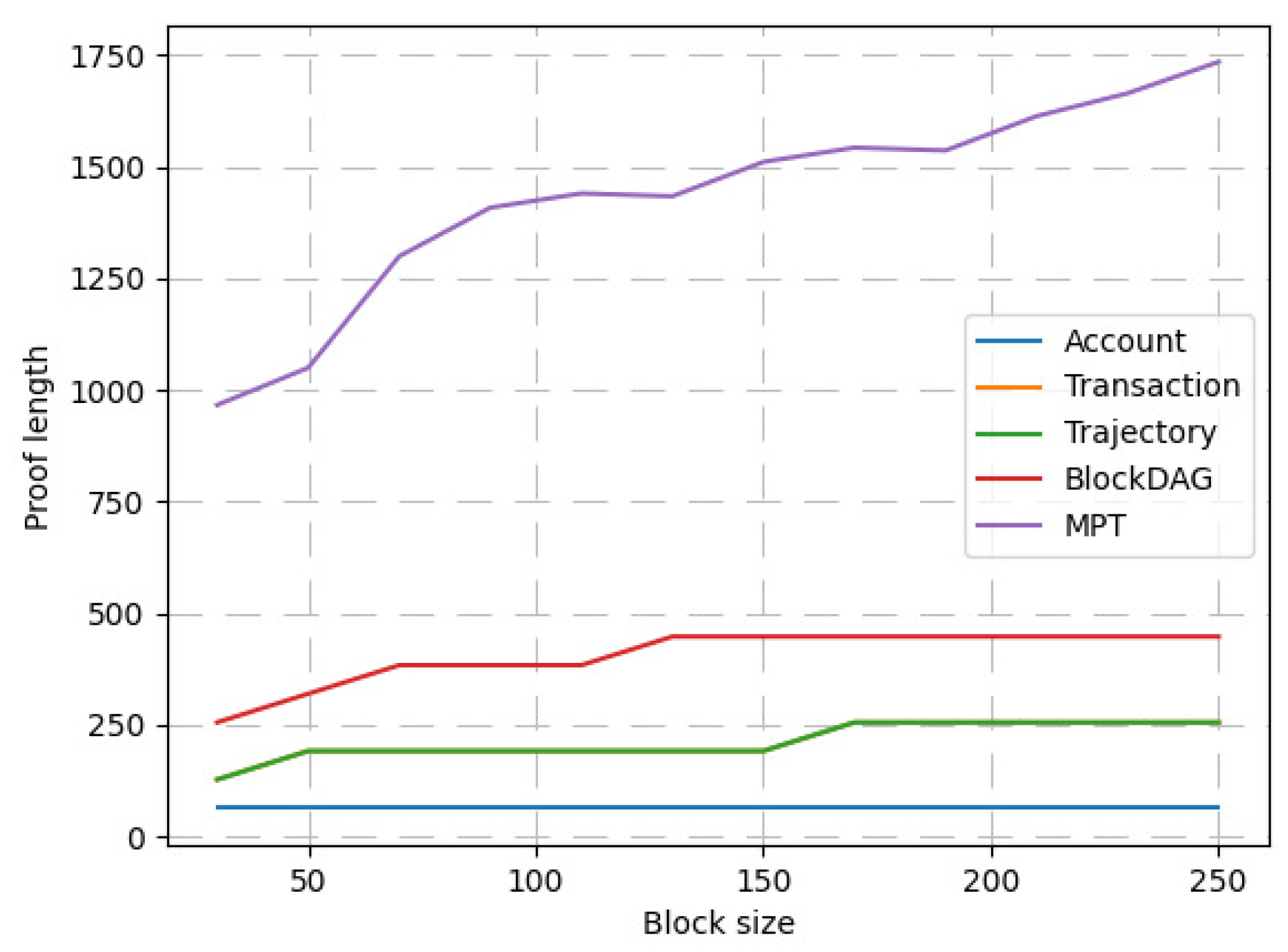
• The length of vector commitment provided by the Verkle tree is related to the depth of the tree, but independent of the width of the tree. Therefore, it should be better than the Merkle tree in performance. However, it is unclear about the difference in proving the performance of Verkle AR*-trees of various sizes, which needs to be further compared in experiments.

All experiments are coded in Python3.7 and performed on a machine with Intel(R) Xeon(R) Gold 2.6 GHz processor and 8 GB RAM. All codes and data can be downloaded from https://github.com/bio-neuroevolution/VRstarTree (accessed on 17 July 2022).

4.2. Result

4.2.1. Spatio-Temporal Query Performance of Verkle AR*-Tree

We set the maximum width of the Verkle AR*-tree to 8. We sampled query region centers from the following mixed Gaussian model in a normalized region composed of latitude, longitude and timestamp. The width of each query cube is sampled on a Gaussian distribution centered at 0.05 and variance at 0.1.

$$p\left(x\right)=\frac{1}{8}\times \sum N(u_i,I)\left(x\right)$$

(5)

where $u_i$ is the eight endpoints of the cube surrounded by <0.33,0.33,0.33> and <0.66,0.66,0.66>. We set the block size from 20 to 160 with an interval of 20. For each block size, we randomly sample 200 query cubes and execute queries on Verkle R*-tree (lack of adaptation), Verkle AR*-tree (adaptive included) and Merkle KD tree [9], respectively. The experiment was run five times, and the average of all experiments was taken as the result, as shown in Figure 7.

Both adaptive Verkle AR*-tree and Verkle R*-tree have better performance than Merkle KD-tree, which is consistent with the experimental results in [34]. Considering that KD-tree itself is only suitable for point data, while R*-tree supports point and regional data. We modify the KD-tree to support regional data: when regional data crosses the KD-tree’s splitting line, we assign the data to both the left and right subtrees. We further randomly select 20% of the pokeman data set, and modify these points into cubes by generating geometric widths through three Gaussian distribution (N (0.001,0.5), N (0.01,0.5), N (0.05,0.5)) with selection probabilities of 0.5, 0.3 and 0.2. After performing the same experiment above, the results are shown in Figure 8.

In Figure 8a, the performance of the KD tree decreases greatly with the increase of block size. For cube data, the left and right subtrees of the node of the Merkle KD-tree have a large number of the overlapping cube, resulting in a larger tree depth with the increase of data. In Figure 8b, the Verkle AR*-tree performs better than Verkle R*-tree, indicating that the Verkle AR*-tree algorithm is also applicable to cube data. In addition, the increase in block size brings more cube data, resulting in more query distribution bias, so Verkle AR*-tree can increase the performance faster than Verkle R*-tree as the block size increases, which is similar to the point query characteristics in Figure 7.

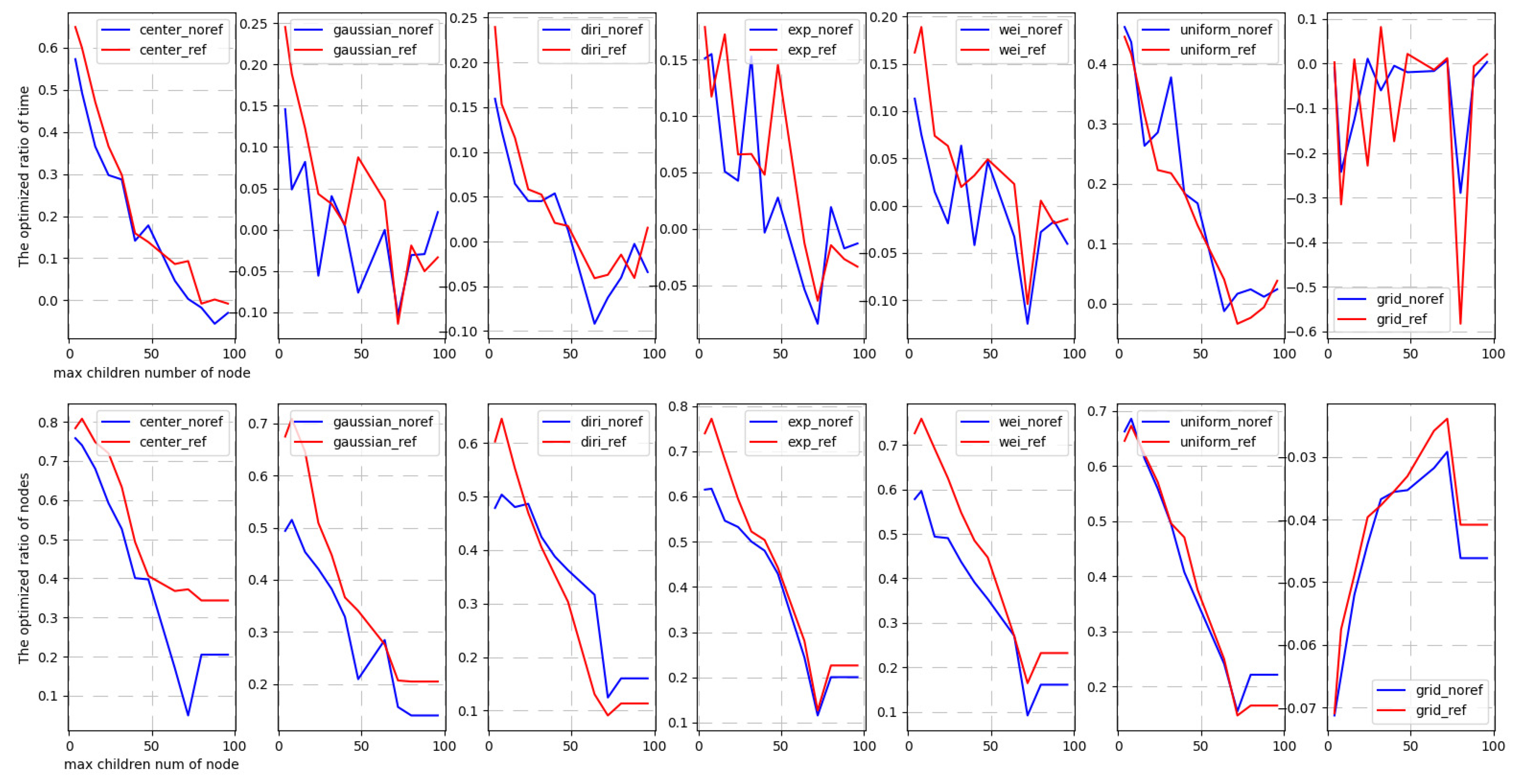
4.2.2. Adaptive Performance Analysis

A Verkle AR*-tree with adaptive ability puts the data accessed with similar frequency and spatially adjacent to the same parent node as much as possible, so as to improve the query performance by reducing the number of node backtracking. Figure 9 shows the number of node accesses of the two algorithms under different block sizes in the previous experiment. It can be seen that the improvement of the Verkle AR*-tree query performance comes from the reduction of the number of access nodes.

However, the performance of adaptive Verkle AR*-tree is greatly affected by query distribution and max children size of the node. We design seven sampling methods for the query window.

• Center sampling. The center of all query windows is fixed in the center of the whole space-time region. the width of each dimension of the query window is obtained by sampling on Gaussian distribution N(0.3,0.05). The exception is that the width of the query window’s time dimension (third dimension) is fixed at 0.5 to allow more blocks to be effectively queried.
• Gaussian sampling. the query distribution is a Gaussian function(the number of center points is 9, and the width of the query window follows the normal distribution with a center value of 0.1 and a variance of 0.05).
• Dirichlet sampling. Both the central position and width of the query window follow the Dirichlet distribution with alpha = 3 and k = 4.
• Exponential sampling: The query center point follows the multivariate exponential distribution with scale = 2, and the width of the query window follows the normal distribution with a center value of 0.1 and variance of 0.05.
• Weibull sampling: The position of the query center follows the Weibull distribution with shape = 5, and the width of the query window follows the normal distribution with a center value of 0.1 and a variance of 0.05.
• Uniform sampling. The uniform sampling generates the center of the query with uniform distribution in the whole spatio-temporal region, and the width of each dimension of the query window is 0.05.
• Grid sampling. We fix a total number of queries, and then divide the whole space into grids according to the number of queries. Each grid just corresponds to a query window. This is an absolute uniform sampling, where uniform sampling is sampling with probability distribution.

In methods 2–3, the sampling location of the previous query is independent of that of the subsequent query, whereas in methods 4–5, the previous query affects the location of the subsequent query. Method 1 can be considered a special case of Gaussian queries, while method 7 can be considered a special case of uniformly distributed queries.

For each of the above sampling methods, we execute the adaptive reconstruction algorithm twice. The first(named non-ref) does not use the historical query frequency, but the second(named ref) does. For the former, lines 10–11 in the realragenodes algorithm are not executed. For each sampling we get 6000 query windows to record the total query time and the number of nodes accessed. We calculate the optimized ratio of access time and the number of nodes accessed, respectively. The optimization ratio is defined by the following formula, where ORT is the optimized ratio of time, TBR is Query time before reconstruction, TAR is Query time after reconstruction, and ORN is the optimized ratio of nodes, NBR is the number of nodes accessed before reconstruction, NAR is the number of nodes accessed after reconstruction.

$$\begin{array}{cc}\hfill ORT& =\frac{(TBR-TAR)}{TBR}\hfill \\ \hfill ORN& =\frac{(NBR-NAR)}{NBR}\hfill \end{array}$$

(6)

The purpose of the experiment is to check the relative performance improvement of the reconstruction algorithm based on query distribution frequency. We set the architectural node number for [4,8,16,24,32,40,48,64,72,80,88,96] and carry out the above experiments. The experimental results are shown in Figure 10.

For center sampling and Gaussian sampling, the reconstruction based on history query frequency is always better than that not used. For uniform sampling and grid sampling, the results of multiple executions show that the difference between the two becomes uncertain.

For four common query distribution samples (Gaussian distribution, Dirichlet distribution, multivariate exponential distribution and Weibull distribution), adaptive algorithms contribute to the performance improvement in all of them. The degree of performance improvement of the four algorithms ($OR{T}_{ref}-OR{T}_{noref}$) is 0.041, 0.022, 0.017, and 0.039, respectively, among which the adaptive algorithm with Gaussian distribution has the best performance.

According to the above experimental results, the applicable scope of the Verkle AR*-tree’s adaptive algorithm is limited. In real applications, it is necessary to accumulate historical query records for a certain period of time, and then decide whether to apply the adaptive algorithm based on the distribution fitting results of these query records.

4.2.3. Performance Analysis of Vector Commitment

In the Merkle tree, the evidence of a value is the complete set of all sibling nodes, while in the Verkle tree, the evidence only needs to be provided along the path of the tree, which reduces the length of proof information accompanying the query. In the experiment, we randomly query 10 times and assume that the minimum proof length required for the valid data in each leaf node is 64 bytes. We compare the cost of the MPT tree and the Verkle tree, and Merkle KD-tree and Verkle AR*-tree proofs, respectively, as shown in Figure 11. Verkle structures always have lower proof overhead than Merkle structures for different tree sizes.

The account information is stored in Verkle Patricia trie (VPT) with location data, and the tree depth is only related to the key of the account, not to the location. In the experiment, the query of the account information obtained the shortest vector proof length, which has little to do with the block size. The Verkle AR*-tree index is used for both transactions and trajectories. The data volume of the two is the same and the data length of each node is uniformly set to 64 bytes, resulting in the overlap of their proof lengths under various block sizes. As the block size increases, their proof length also increases, but they are smaller than MPT and Merkle KD-tree.

5. Discussion

In the first experiment, we performed queries with no committed proof overhead. In this case, transactions are organized into R*-tree in each blockchain, and the size of the tree is constrained by the size of a block. The spatial objects stored in the blockchain are three-dimensional, longitude, latitude and time dimension, and are normalized to 0–1. We do not care about the cost of block construction, but about the performance of real-time spatio-temporal region query in the block. Although R*-tree is reported to be more suitable for indexing large-scale disk storage data, we can see that the memory R*-tree under the block capacity limit also has better performance. Whether for point objects or cube objects, the query performance is better than the existing Merkle KD tree.

In the second experiment, we compare the query performance of our proposed adaptive R*-tree and the existing R*-tree. The experimental results show that the performance improvement of the adaptive R*-tree is mainly due to the reduction of the number of visited nodes, which is affected by the historical query distribution and the maximum child node capacity of the tree, so it is not always effective. In addition, the adaptive algorithm needs to reconstruct the whole tree from bottom to top regularly. In our experiment, the overhead of block locking during reconstruction is ignored.

In the third experiment, we added vector commitment to the blockchain. The queried object and corresponding proof information are obtained in each query, which can help the client verify the authenticity of the data. The verification consists of three separate processes. The first is the generation process of Verkle vector commitment, which occurs during block creation and is generated when each spatio-temporal object is inserted; The second is to return the commitment information together with the query results; The third is the authentication process that takes place on the client. Among the three processes, the second one has the greatest impact on the performance and the length of the proof information determines the performance of the process. In Merkle proof, the proof length is related to the size of the whole tree, while in Verkle proof, the proof length is related to the depth of the tree.

We have implemented three types of data storage in the blockchain, including accounts with the last location, transaction information and trajectories of each account. The former uses a Verkle Patricia Tree and the latter two use Verkle R*-tree. We compare these three trees with the Merkle Patricia tree (MPT) and the Merkle KD tree in Block-DAG [9]. In the experiment, we do 10 random queries on each tree and calculate the proof length. The results show that the proof based on Verkle is better than Merkle’s proof in various tree structures.

6. Conclusions and Future Work

In this paper, we study the technology of storing and querying spatio-temporal data in blockchain without adding additional storage. We propose a Verkle AR*-tree, in which vector proofs of Verkle trees are integrated with the R*-tree. Compared with the existing Merkle KD-tree method, we extend the spatial index from point to the cube, and improve the performance of spatio-temporal query. We add adaptive ability based on query distribution to R*-tree, and the query performance exceeds that of the existing R*-tree even when the query distribution is not uniform. We use the vector commitment of the Verkle tree to provide proof for spatio-temporal queries and its proof efficiency is also higher than the Merkle tree. Based on the above technology, we added three spatial data indexes to the blockchain, including the last location of the account based on the VPT tree, transaction information and trajectories of the account based on the Verkle AR*-tree.

In the future, we would like to further implement the parallel version of the Verkle AR*-tree and try to apply it in applications.

References

1. Xu, M.; Chen, X.; Kou, G. A systematic review of blockchain. Financ. Innov. 2019, 5, 27. [Google Scholar] [CrossRef] [Green Version]
2. Casino, F.; Dasaklis, T.K.; Patsakis, C. A systematic literature review of blockchain-based applications: Current status, classification and open issues. Telemat. Inform. 2019, 36, 55–81. [Google Scholar] [CrossRef]
3. Worley, C.; Skjellum, A. Blockchain Tradeoffs and Challenges for Current and Emerging Applications: Generalization, Fragmentation, Sidechains, and Scalability. In Proceedings of the 2018 IEEE International Conference on Internet of Things (iThings) and IEEE Green Computing and Communications (GreenCom) and IEEE Cyber, Physical and Social Computing (CPSCom) and IEEE Smart Data (SmartData), Halifax, NS, Canada, 30 July–3 August 2018; pp. 1582–1587. [Google Scholar] [CrossRef]
4. Nakamoto, S. Bitcoin: A Peer-to-Peer Electronic Cash System. Available online: https://bitcoin.org/bitcoin.pdf (accessed on 22 May 2022).
5. Back, A.; Corallo, M.; Dashjr, L.; Friedenbach, M.; Maxwell, G.; Miller, A.; Poelstra, A.; Timón, J.; Wuille, P. Enabling Blockchain Innovations with Pegged Sidechains. Available online: https://blockstream.com/sidechains.pdf (accessed on 22 May 2022).
6. Vujičić, D.; Jagodić, D.; Ranđić, S. Blockchain technology, bitcoin, and Ethereum: A brief overview. In Proceedings of the 2018 17th International Symposium Infoteh-Jahorina (INFOTEH), East Sarajevo, Bosnia and Herzegovina, 21–23 March 2018; pp. 1–6. [Google Scholar] [CrossRef]
7. Helmer, S.; Roggia, M.; El Ioini, N.; Pahl, C. EthernityDB – Integrating Database Functionality into a Blockchain. In Proceedings of the European Conference on Advances in Databases and Information Systems, Budapest, Hungary, 2–5 September 2018; Springer: Berlin/Heidelberg, Germany, 2018; pp. 37–44. [Google Scholar] [CrossRef]
8. Sompolinsky, Y.; Wyborski, S.; Zohar, A. PHANTOM GHOSTDAG: A Scalable Generalization of Nakamoto Consensus: September 2, 2021. In Proceedings of the 3rd ACM Conference on Advances in Financial Technologies, Arlington, VA, USA, 26–28 September 2021; pp. 57–70. [Google Scholar]
9. Nurgaliev, I.; Muzammal, M.; Qu, Q. Enabling Blockchain for Efficient Spatio-Temporal Query Processing. In Proceedings of the International Conference on Web Information Systems Engineering, Melbourne, VIC, Australia, 20–24 October 2018; Springer: Berlin/Heidelberg, Germany, 2018; pp. 36–51. [Google Scholar]
10. Kuszmaul, J. Verkle trees. Available online: https://math.mit.edu/research/highschool/primes/materials/2018/Kuszmaul.pdf (accessed on 22 May 2022).
11. Ahn, H.K.; Mamoulis, N.; Wong, H. A Survey on Multidimensional Access Methods. Available online: https://dspace.library.uu.nl/bitstream/handle/1874/2491/2001-14.pdf (accessed on 22 May 2022).
12. Samet, H. The Quadtree and Related Hierarchical Data Structures. ACM Comput. Surv. 1984, 16, 187–260. [Google Scholar] [CrossRef] [Green Version]
13. Ooi, B.; Mcdonell, K.; Sacks-davis, R. Spatial kd-tree: An indexing mechanism for spatial databases. In Proceedings of the IEEE International Computer Software and Applications Conference, Tokyo, Japan, 5–6 October 1987; pp. 433–438. [Google Scholar]
14. Ohsawa, Y.; Sakauchi, M. The BD-Tree - A New N-Dimensional Data Structure with Highly Efficient Dynamic Characteristics. In Proceedings of the IFIP 9th World Computer Congress, Paris, France, 19–23 September 1983; pp. 539–544. [Google Scholar]
15. Tao, Z.; Cheng, C.; Pan, Z.; Shi, J. Generation and applications of a multi-resolution BSP tree. J. Softw. 2001, 12, 117–125. [Google Scholar]
16. Li, C.; Wu, Z.; Wu, P.; Zhao, Z. An Adaptive Construction Method of Hierarchical Spatio-Temporal Index for Vector Data under Peer-to-Peer Networks. ISPRS Int. J. Geo-Inf. 2019, 8, 512. [Google Scholar] [CrossRef] [Green Version]
17. Beckmann, N.; Kriegel, H.P.; Schneider, R.; Seeger, B. The R*-tree: An efficient and robust access method for points and rectangles. ACM SIGMOD 1990, 19, 322–331. [Google Scholar] [CrossRef]
18. Šumák, M.; Gurský, P. R++-Tree: An Efficient Spatial Access Method for Highly Redundant Point Data. In New Trends in Databases and Information Systems; Springer: Berlin/Heidelberg, Germany, 2014; pp. 37–44. [Google Scholar]
19. Shekhar, S.; Xiong, H.; Zhou, X. (Eds.) R-Tree. In Encyclopedia of GIS; Springer: Berlin/Heidelberg, Germany, 2017; p. 1805. [Google Scholar] [CrossRef]
20. Gunther, O. The design of the cell tree: An object-oriented index structure for geometric databases. In Proceedings of the Fifth International Conference on Data Engineering, Los Angeles, CA, USA, 6–10 February 1989; pp. 598–605. [Google Scholar] [CrossRef]
21. Kamel, I.; Faloutsos, C. Hilbert R-Tree: An Improved R-Tree Using Fractals. In Proceedings of the 20th International Conference on Very Large Data Bases (VLDB ’94), Santiago de Chile, Chile, 12–15 September 1994; pp. 500–509. [Google Scholar]
22. Altarawneh, A.; Herschberg, T.; Medury, S.; Kandah, F.; Skjellum, A. Buterin’s Scalability Trilemma viewed through a State-change-based Classification for Common Consensus Algorithms. In Proceedings of the 2020 10th Annual Computing and Communication Workshop and Conference (CCWC), Las Vegas, NV, USA, 6–8 January 2020; pp. 727–736. [Google Scholar] [CrossRef]
23. Wan, L. A Query Optimization Method of Blockchain Electronic Transaction Based on Group Account. In Proceedings of the International Conference on Big Data Analytics for Cyber-Physical-Systems, Shanghai, China, 28–29 December 2021; Springer: Berlin/Heidelberg, Germany, 2021; pp. 1358–1364. [Google Scholar] [CrossRef]
24. Sompolinsky, Y.; Zohar, A. PHANTOM: A Scalable BlockDAG Protocol. In Proceedings of the 3rd ACM Conference on Advances in Financial Technologies, Arlington, VA, USA, 26–28 September 2021. [Google Scholar]
25. Szydlo, M. Merkle Tree Traversal in Log Space and Time. In International Conference on the Theory and Applications of Cryptographic Techniques; Springer: Berlin/Heidelberg, Germany, 2004; pp. 541–554. [Google Scholar]
26. Kamel Boulos, M.N.; Wilson, J.T.; Clauson, K.A. Geospatial blockchain: Promises, challenges, and scenarios in health and healthcare. Int. J. Health Geogr. 2018, 17, 25. [Google Scholar]
27. Liu, H.; Tai, W.; Wang, Y.; Wang, S. A Blockchain-Based Spatial Data Trading Framework. Preprint. 2021. Available online: https://www.researchgate.net/publication/348709925_A_Blockchain-Based_Spatial_Data_Trading_Framework (accessed on 22 May 2022).
28. Sun, Y.; Zhang, L.; Feng, G.; Yang, B.; Cao, B.; Imran, M. Performance Analysis for Blockchain Driven Wireless IoT Systems Based on Tempo-Spatial Model. In Proceedings of the 2019 International Conference on Cyber-Enabled Distributed Computing and Knowledge Discovery (CyberC), Guilin, China, 17–19 October 2019; pp. 348–353. [Google Scholar] [CrossRef]
29. Demenkov, M.; Demenkova, E.; Shishmanova, S. Application of blockchain technology for storage information on spatial objects. Vestn. Astrakhan State Tech. Univ. Ser. Manag. Comput. Sci. Inform. 2019, 1, 61–72. [Google Scholar] [CrossRef]
30. Qu, Q.; Nurgaliev, I.; Muzammal, M.; Jensen, C.S.; Fan, J. On spatio-temporal blockchain query processing. Future Gener. Comput. Syst. 2019, 98, 208–218. [Google Scholar] [CrossRef]
31. Mouratidis, K.; Sacharidis, D.; Pang, H.H. Partially materialized digest scheme: An efficient verification method for outsourced databases. VLDB J. 2009, 18, 363–381. [Google Scholar] [CrossRef]
32. Kriegel, H.P.; Kunath, P.; Renz, M. R*-Tree. In Encyclopedia of GIS; Shekhar, S., Xiong, H., Eds.; Springer: Berlin/Heidelberg, Germany, 2008; pp. 987–992. [Google Scholar] [CrossRef]
33. Pagel, B.U.; Six, H.W.; Toben, H.; Widmayer, P. Towards an Analysis of Range Query Performance in Spatial Data Structures. In Proceedings of the Twelfth ACM SIGACT-SIGMOD-SIGART Symposium on Principles of Database Systems, Washington, DC, USA, 25–28 May 1993; pp. 214–221. [Google Scholar] [CrossRef]
34. Greene, D. An implementation and performance analysis of spatial data access methods. In Proceedings of the Fifth International Conference on Data Engineering, Los Angeles, CA, USA, 6–10 February 1989; pp. 606–615. [Google Scholar] [CrossRef]
Figure 1. R-tree and R*-tree. (a) R-tree. (b) R*-tree. (c) R*-tree with query window.
Ijgi 11 00409 g001
Figure 2. Merkle tree and Verkle tree. (a) Merkle tree. (b) Verkle tree.
Ijgi 11 00409 g002
Figure 3. Verkle Patricia Trie.
Ijgi 11 00409 g003
Figure 4. Transaction information stored in Verkle AR*-tree.
Ijgi 11 00409 g004
Figure 5. Schematics of split algorithm.
Ijgi 11 00409 g005
Figure 6. Trajectories stored in Verkle R*-tree.
Ijgi 11 00409 g006
Figure 7. Query performance under different block sizes for point objects.
Ijgi 11 00409 g007
Figure 8. Query performance under different block sizes for cube objects. (a) Merkle KD-tree and Verkle AR*-tree. (b) Verkle R*-tree and Verkle AR*-tree.
Ijgi 11 00409 g008
Figure 9. The number of node accesses of the two algorithms under different block sizes.
Ijgi 11 00409 g009
Figure 10. Query performance of the two algorithms under different query distribution.
Ijgi 11 00409 g010
Figure 11. Performance Analysis of Vector Commitment.
Ijgi 11 00409 g011
Publisher’s Note: MDPI stays neutral with regard to jurisdictional claims in published maps and institutional affiliations.