A Progressive Simplification Method for Buildings Based on Structural Subdivision

Abstract

Building simplification is an important research area in automatic map generalization. Up to now, many approaches have been proposed by scholars. However, in the continuous transformation of scales for buildings, keeping the main shape characteristics, area, and orthogonality of buildings are always the key and difficult points. Therefore, this paper proposes a method of progressive simplification for buildings based on structural subdivision. In this paper, iterative simplification is adopted, which transforms the problem of building simplification into the simplification of the minimum details of building outlines. Firstly, a top priority structure (TPS) is determined, which represents the smallest detail in the outline of the building. Then, according to the orthogonality and concave–convex characteristics, the TPS are classified as 62 subdivisions, which cover the local structure of the building polygon. Then, the subdivisions are divided into four simplification types. The building is simplified to eliminate the TPS continuously, retaining the right-angle characteristics and area as much as possible, until the results satisfy the constraints and rules of simplification. A topographic dataset (1:1 K) collected from Kadaster was used for our experiments. In order to evaluate the algorithm, many tests were undertaken, including tests of multi-scale simplification and simplification of typical buildings, which indicate that this method can realize multi-scale presentation of buildings. Compared with the existing simplification methods, the comparison results show that the proposed method can simplify buildings effectively, which has certain advantages in keeping shape characteristics, area, and rectangularity.

1. Introduction

Building (group) simplification is an important issue in automatic cartographic generalization of large-scale maps [1,2,3]. It aims to represent buildings more concisely depending on the map scale or theme, with requirements of legibility and a good representation of reality [4]. As the important man-made objects on the topographic maps, buildings have some unique shape characteristics that distinguish them from natural objects, such as rectangularity and orthogonality. In consequence, many simplification algorithms for buildings have been proposed in recent years for this aim. Building simplification could reduce the cognitive burden of map users on smaller scales, which help them acquire implied relationships. Moreover, the progressive simplification of buildings could provide users with a “continuous” and “stepless zoom” visual experience. In addition to its application in traditional cartography, the simplification of buildings also helps to simplify the outline of buildings extracted from high-resolution remote sensing images, making the shape of buildings more regular [5]. In the identification of urban functional areas, the shapes of buildings at different scales are the important basis for mining spatial information [6,7]. Building simplification is usually conducted on a single building, largely independent of contextual information. Additionally, it sometimes can be conducted separately in the process of building map generalization [8]. This paper just focuses on individual building simplification of outlines.

Simplification of individual buildings is the basic operation in cartographic generalization [2]. The problem of building simplification is computing a simplification of a given subdivision, subject to various constraints that affect the retention of important features and the aesthetics of the simplified buildings [9]. There are some basic requirements in building simplification. First, the simplified buildings should be legible [10]. As the scale reduces, the short edges whose length are smaller than the specified threshold are eliminated. Second, preserving or enhancing the main characteristics of a building is another important constraint, including position, size, orientation, and orthogonality. Furthermore, the typical characteristic of shape must be preserved, keeping the shape similar before and after simplification. For example, if the outline of a building looks like the letter E, the simplified building should be consistent in terms of shape characteristics. Especially, the simplified buildings are gradual in shape in continuous scale transformation of maps. Third, the simplification method can be applied to different types of buildings. For example, some methods just assume buildings with orthogonal characteristics [11,12,13]. However, in the real word, buildings not only have orthogonal characteristics, but also have non-orthogonal characteristics [14]. Several of the existing methods in this field are restricted in applicability due to rarely classifying and simplifying the structural types of buildings with full coverage.

Hence, in the continuous transformation of scales for buildings, keeping the main characteristics, area, and orthogonality of building outlines are always the key and difficult points, especially for some buildings with non-orthogonal characteristics and complicated shapes. Considering that the essence of building simplification is to delete, displace, and construct the vertices under the principle of simplification [15], building simplification is a process of deleting and integrating the minimal details constantly. We propose a progressive building simplification approach based on structural subdivision. Iterative simplification is adopted, which transforms the problem of building simplification into the simplification of the minimum details of building outlines. Firstly, a top priority structure (TPS) is determined, which represents the smallest detail in the outline of the building. Then, according to the orthogonality and concave–convex characteristics of the TPS, the simplification type is determined in four simplification types. The building is simplified to eliminate the TPS continuously, retaining the shape, orthogonality, and area as much as possible, until the building meets the simplification requirements.

2. Related Works

The simplification of buildings is a classic problem in map generalization, which is the basic element of generalization when the “raw” information is too intricate or abundant to be fully reproduced to the scale of the map as it stands. At the beginning of 1940s, Wright (1942) [16] related to the scientific reliability of maps which in a decisive way depends on generalization. According to him, simplification and amplification are the two elements of generalization. Raisz (1962) [17] broadened the views on generalization. In his opinion, there are no particular rules of generalization, which is a combination of three processed: association, omission, and simplification. Referring to Robinson et al. (1978) [18], selection and the four elements of cartographic generalization, simplification, classification, symbolization, and induction, are applied during the elaboration of maps. Ratajski (1989) [19] supported Robinson’s stance by distinguishing two types of generalization: qualitative and quantitative. McMaster and Shea (1992) [20] generated a model for digital generalization, and tried to answer three questions: why, when, and how one should be generalized.

According to Lee et al. (2005) [21] and Wang et al. (2005) [22], an effective way to simplify an individual building usually considers the following rules:

• A building must be simplified if it contains edges shorter than a specified length.
• The morphological characteristics must be as similar as possible.
• The visual center of the building remains unchanged.
• The orthogonal shape should be preserved or enhanced.
• The area of the building should be approximately the same.
• If a building has been simplified to a rectangle or quadrilateral, then it will not be simplified further.

More than that, the rules of building simplification are more enriched nowadays. Keeping the area of buildings should be determined according to the mapping purpose or specific situations. For small buildings, enlargement is a typical procedure. On the other hand, it is important to retain the area for cadastral purposes. Moreover, non-rectangular shapes and even circular shapes of buildings are common in many cities. It is necessary to improve the adaptability of simplification algorithms for various buildings.

Currently, according to the type of spatial data, two kinds of building simplification methods exist: the raster-based simplification method and vector-based simplification method. Since this paper focuses on vector-based methods, the raster-based methods will not be introduced in detail. Vector-based methods can be classified into local-structure-based, template-based, and combined-based.

In local-structure-based methods, the buildings are simplified by removing unimportant or small details. An approach is presented for the simplification of building ground plans, which is based on the techniques of half-space modeling and cell decomposition [23]. Haunert and Wolff (2008) [3] proposed a heuristic and an integer programming formulation to simplify buildings. Buchin et al. (2011) [24] introduced an operation of edge-move for polygon simplification. The least squares method is also used for building simplification [2,12,25,26]; Meijers (2016) [27] presented a conceptual simple algorithm to simplify building outlines based on offset curves obtained from the straight skeleton. However, the process of acquiring skeleton will reduce efficiency The preservation of right angles is one of the main constraints involved in the simplification of buildings [2]. A simplification method of building polygons with right-angled turns is discussed, considering the preservation of right-angled shapes and areas [11]. A multi-agent approach is applied to model cartographic objects and treatment in generalization, including the simplification of building outlines [28,29]. Self-optimizing techniques have already been studied for an agent system performing generalization [30]. Jin et al. (2020) [31] provided a constrained building boundary simplification method based on the partial total least squares, which could obtain smaller geometric displacements of buildings than the classic least-squares-based fitting method. A simplification algorithm is designed by judging edge structure features of four or five adjacent points [15,32,33], which achieves simplification of various types of buildings. Yin et al. (2020) [34] proposed a simplification method of feature edge reconstruction for building polygons with fuzzy outlines. Some types of software used for map generalization have more functionality to realize building simplification [35,36,37].

In template-based methods, the building is simplified by replacing with predefined templates, which are similar to the building with a simpler form. Rainsford and Mackaness (2002) [4] proposed a building simplification method based on shape matching, which preserves the shape characteristics and area after simplification with strong practicability [38,39,40,41]. However, due to the limitation of the template library type, it is not ideal for polygon simplification with complex structures. In combined-based methods, different algorithms are combined to achieve the building simplification task. Considering numerous algorithms to simplify buildings, Yang et al. (2021) [42] presented a hybrid approach that identifies the best simplified representation of a building among four existing algorithms to generate simplification candidates with a backpropagation neural network. Wei et al. (2021) [8] proposed a combined building simplification approach based on local structure classification. The local structures are classified and operated by considering the buildings’ orthogonal and non-orthogonal characteristics. However, the individual building simplification is the foundation of combined building simplification approaches.

Recently, superpixel and deep learning methods have been used to simplify polygons. Shen et al. (2018; 2019) [14,43] proposed a new method to simplify polygons using superpixel segmentation. Sester et al. (2018) [44] applied a deep convolution network to cartographic generalization tasks. Feng et al. (2019) [45] improved the existing deep learning network and proved the feasibility of the method. The simplification method based on machine learning is highly automated, but it is highly dependent on the quality of the sample training set.

3. Methodology

Similar to the iterative simplification method of lines proposed by Douglas and Pucker (1973) [46], the basic idea of the simplification is as follows: The building simplification is the process of reducing the small details of outlines under the constraints of the simplification. A minimum structure of outlines, which presents the minimum detail to be simplified preferentially, can be determined each time. The building is simplified by determining and simplifying the minimum structure iteratively. As Figure 1 shows, the original building in Figure 1a is simplified to Figure 1b after simplifying the minimum structure twice. The main works of our approach are determination and classification of the minimum structure. Then, the simplification algorithm of minimum structure is put forward, respectively.

Figure 1. The basic idea of the proposed method.

3.1. Basic Concepts

For better description, this paper defines the following parameters:

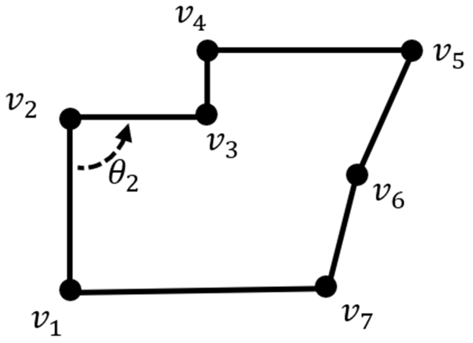
In this paper, suppose for any building polygon $B_v$, which is composed by a set of vertices $\left\{v_1,v_2,\cdots ,v_n\right\}$. The angle set of vertices is $\left\{{\theta }_1,{\theta }_2,\cdots ,{\theta }_n\right\}$. The angle at vertex $v_i$ is supposed as ${\theta }_i$, denoted as the angle of edge $v_{i-1}{v}_i$ rotates counterclockwise around vertex $v_i$ to edge $v_i{v}_{i+1}$, and ${\theta }_i\in \left[0^{°},{360}^{°}\right]$, e.g., ${\theta }_2$ is the angle of $v_2$ in Figure 2. The length of each edge of $B_v$ is $\left\{\left|v_1{v}_2\left|,\right|v_2{v}_3\left|,\cdots ,\right|v_{n-1}{v}_n\left|,\right|v_n{v}_1\right|\right\}$. The types of local structures are distinguished according to the convexity–concavity and orthogonality of vertices. Thus, flat-angled vertex, orthogonal vertex, non-orthogonal vertex, convex vertex, and concave vertex are defined as followed. $\delta$ is a tolerance range in Table 1 and $\delta ={10}^{°}$ in general.

Figure 2. The example of vertices.

Table 1. Parameter description.

Parameters	Description	Denoted
A tolerance range	A tolerance that allows approximate right-angled angle or flat angle to strict 90° or 180° [26].	$\delta$
Minimum granularity	The actual distance corresponding to the minimum length that human eyes can distinguish on the map [10,15].	$\epsilon$
The length of the shortest edge	The length of the shortest edge in the building polygon.	$MinLen$

Flat-angled vertex (FV): suppose the angle at vertex $v_i$ in $B_v$ as ${\theta }_i$, if $\left|{180}^{°}-{\theta }_i\right|<\delta$, then $v_i$ is a flat-angled vertex, e.g., vertex $v_6$ in Figure 2.

Orthogonal vertex (OV): suppose the angle at vertex $v_i$ in $B_v$ as ${\theta }_i$, if $\left|{90}^{°}-{\theta }_i\right|\le \delta$ or $\left|{270}^{°}-{\theta }_i\right|\le \delta$, then $v_i$ is an orthogonal vertex, e.g., vertex $v_1$ in Figure 2.

Non-orthogonal vertex (NV): suppose the angle at vertex $v_i$ in $B_v$ as ${\theta }_i$, if $\left|{90}^{°}-{\theta }_i\right|>\delta$ and $\left|{270}^{°}-{\theta }_i\right|>\delta$, then $v_i$ is a non-orthogonal vertex, e.g., vertex $v_5$ in Figure 2.

Therefore, define $f_{ort}\left(v_i\right)$ to describe the orthogonality of $v_i$, $v_i\in B_v$:

$$f_{ort}\left(v_i\right)=\left\{\begin{array}{c}OV,\left|{90}^{°}-{\theta }_i\right|\le \delta \cup \left|{270}^{°}-{\theta }_i\right|\le \delta \\ NV,\left|{90}^{°}-{\theta }_i\right|>\delta \cap \left|{270}^{°}-{\theta }_i\right|>\delta \end{array}\right.$$

(1)

Convex vertex (CVV): suppose the angle at vertex $v_i$ in $B_v$ as ${\theta }_i$, if ${\theta }_i<{180}^{°}$, then $v_i$ is a convex vertex, e.g., vertex $v_2$ in Figure 2.

Concave vertex (CCV): suppose the angle at vertex $v_i$ in $B_v$ as ${\theta }_i$, if ${\theta }_i>{180}^{°}$, then $v_i$ is a concave vertex, e.g., vertex $v_3$ in Figure 2.

Therefore, define $f_{con}\left(v_i\right)$ to describe the concave–convex of $v_i$, $v_i\in B_v$:

$$f_{con}\left(v_i\right)=\left\{\begin{array}{c}CVV,{\theta }_i<{180}^{°} \\ CCV,{\theta }_i>{180}^{°} \end{array}\right.$$

(2)

3.2. Definition of Top Priority Vertex and Structure

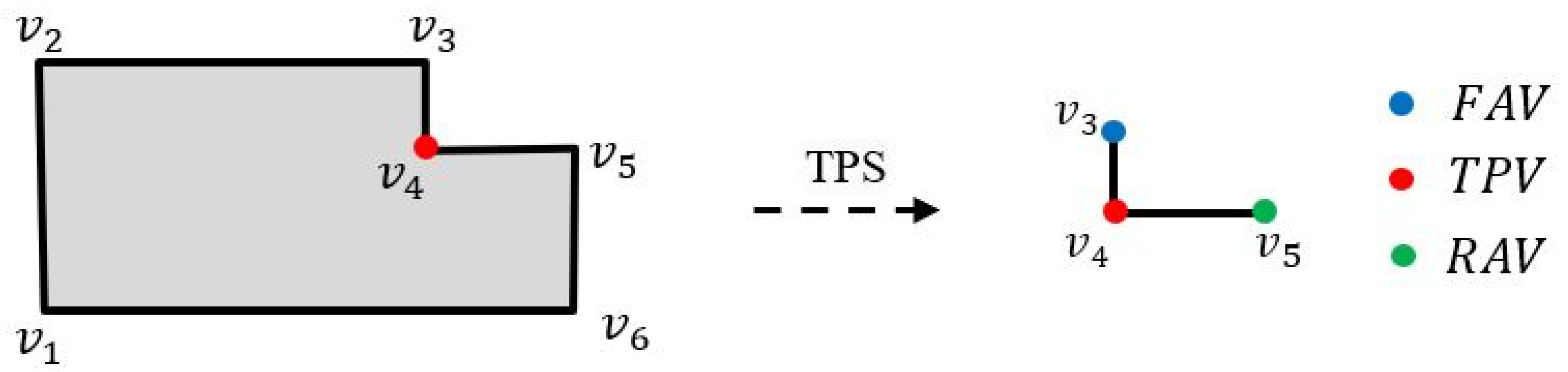
Simplification is the process of reducing the complexity of a geometric shape by eliminating detail [47]. Herein, if a building should be simplified, we define the top-priority-structure (TPS) as the minimal detail to be simplified preferentially. The TPS consists of the top-priority-vertex (TPV) and its two adjacent vertices. According to the sequence of buildings vertices, the two adjacent vertices are distinguished as Front-Adjacent-Vertex (FAV) and Rear-Adjacent-Vertex (RAV). The TPV is determined using two steps:

Step 1: Find the edge with the shortest length of building polygon, denoted as $\left|v_i{v}_j\right|$, in which $v_i$ and $v_j$ are adjacent vertices, and $i<j$.

Step 2: Compare the “structural areas” of $v_i$ and $v_j$, and select the vertex with the smaller structural area as TPV. If the “structural areas” of $v_i$ and $v_j$ are equivalent, select $v_i$ as the TPV.

Suppose the structural area of the vertex $v_i$ in $B_v$ is denoted as $Str{A}_i$, the lengths of the two adjacent edges are $\left|v_{i-1}{v}_i\right|$ and $\left|v_i{v}_{i+1}\right|$, respectively, and the angle at vertex $v_i$ is denoted as ${\theta }_i$, then the structural area of $v_i$ is

$$Str{A}_i=\left|v_{i-1}{v}_i\right|\left|v_i{v}_{i+1}\right|·\left|\sin {\theta }_i\right|$$

(3)

Take the $B_v=\left\{v_1,v_2,\cdots ,v_7\right\}$ in Figure 3, which should be simplified, as an example. Step 1, find the shortest edge $\left|v_3{v}_4\right|$ by calculating the length of polygon edges. Step 2, compare the structural area of $v_3$ and $v_4$, as Figure 3 shows.

$$Str{A}_3=\left|v_2{v}_3\right|\left|v_3{v}_4\right|·\left|\sin {\theta }_3\right|=\left|v_2{v}_3\right|\left|v_3{v}_4\right|$$

(4)

$$Str{A}_4=\left|v_3{v}_4\right|\left|v_4{v}_5\right|·\left|\sin {\theta }_4\right|=\left|v_3{v}_4\right|\left|v_4{v}_5\right|$$

(5)

Figure 3. Determination of the TPV and TPS.

Therein, ${\theta }_3$ and ${\theta }_4$ are 90°and 270°, respectively. $\left|v_2{v}_3\right|>\left|v_4{v}_5\right|$, therefore, $Str{A}_3>Str{A}_4$. The $v_4$ is determined as TPV (indicated by red point), and the local structure $\{v_3,v_4,v_5\}$ is the TPS, which presents the minimal details in the building polygon. $v_3$ is FAV (indicated by blue point) and $v_5$ is RAV (indicated by green point).

3.3. Classification of TPS

As buildings have different shapes, classifying TPS is the basis of the simplification operation. There are three vertices in the TPS, which are FAV, TPV, and RAV. We distinguish the TPS with the concave–convex and orthogonality of the three vertices, as Table 2 shows.

Table 2. Classification of TPS with concave–convex and orthogonality.

		Type 1			Type 2	Type 3		Type 4
		$\mathit{F}\mathit{A}\mathit{V}=\mathit{O}\mathit{V}$ $\mathit{T}\mathit{P}\mathit{V}=\mathit{O}\mathit{V}$ $\mathit{R}\mathit{A}\mathit{V}=\mathit{O}\mathit{V}$	$\mathit{F}\mathit{A}\mathit{V}=\mathit{O}\mathit{V}$ $\mathit{T}\mathit{P}\mathit{V}=\mathit{O}\mathit{V}$ $\mathit{R}\mathit{A}\mathit{V}=\mathit{N}\mathit{V}$	$\mathit{F}\mathit{A}\mathit{V}=\mathit{N}\mathit{V}$ $\mathit{T}\mathit{P}\mathit{V}=\mathit{O}\mathit{V}$ $\mathit{R}\mathit{A}\mathit{V}=\mathit{O}\mathit{V}$	$\mathit{F}\mathit{A}\mathit{V}=\mathit{N}\mathit{V}$ $\mathit{T}\mathit{P}\mathit{V}=\mathit{O}\mathit{V}$ $\mathit{R}\mathit{A}\mathit{V}=\mathit{N}\mathit{V}$	$\mathit{F}\mathit{A}\mathit{V}=\mathit{N}\mathit{V}$ $\mathit{T}\mathit{P}\mathit{V}=\mathit{N}\mathit{V}$ $\mathit{R}\mathit{A}\mathit{V}=\mathit{O}\mathit{V}$	$\mathit{F}\mathit{A}\mathit{V}=\mathit{O}\mathit{V}$ $\mathit{T}\mathit{P}\mathit{V}=\mathit{N}\mathit{V}$ $\mathit{R}\mathit{A}\mathit{V}=\mathit{N}\mathit{V}$	$\mathit{F}\mathit{A}\mathit{V}=\mathit{O}\mathit{V}$ $\mathit{T}\mathit{P}\mathit{V}=\mathit{N}\mathit{V}$ $\mathit{R}\mathit{A}\mathit{V}=\mathit{O}\mathit{V}$	$\mathit{F}\mathit{A}\mathit{V}=\mathit{N}\mathit{V}$ $\mathit{T}\mathit{P}\mathit{V}=\mathit{N}\mathit{V}$ $\mathit{R}\mathit{A}\mathit{V}=\mathit{N}\mathit{V}$
$FAV=\mathrm{CVV}$ $TPV=\mathrm{CVV}$ $RAV=\mathrm{CVV}$		—
$FAV=\mathrm{CVV}$ $TPV=\mathrm{CVV}$ $RAV=\mathrm{CCV}$
$FAV=\mathrm{CCV}$ $TPV=\mathrm{CVV}$ $RAV=\mathrm{CVV}$
$FAV=\mathrm{CCV}$ $TPV=\mathrm{CVV}$ $RAV=\mathrm{CCV}$
$FAV=\mathrm{CVV}$ $TPV=\mathrm{CCV}$ $RAV=\mathrm{CVV}$
$FAV=\mathrm{CCV}$ $TPV=\mathrm{CCV}$ $RAV=\mathrm{CVV}$
$FAV=\mathrm{CVV}$ $TPV=\mathrm{CCV}$ $RAV=\mathrm{CCV}$
$FAV=\mathrm{CCV}$ $TPV=\mathrm{CCV}$ $RAV=\mathrm{CCV}$		—

According to the Table 2, the TPS are classified as 62 subclasses, which cover the local structure of the building polygon. In order to keep the shape characteristics simplified, the 62 subclasses are divided into four types of simplification, which consist of 12 simplification cases. The four types of simplification are the following:

• Simplification type 1: TPV is OV, and there is OV in the adjacent two vertices:

$$TPS\in \left\{f_{ort}\left(TPV\right)=\mathrm{OV}, f_{ort}\left(FAV\right)=OV\cup f_{ort}\left(RAV\right)=OV\right\}$$

• Simplification type 2: TPV is OV, and there is no OV in the adjacent two vertices:

$$TPS\in \left\{f_{ort}\left(TPV\right)=\mathrm{OV}, f_{ort}\left(FAV\right)=NV\cap f_{ort}\left(RAV\right)=NV\right\}$$

• Simplification type 3: TPV is NV, and the orthogonality of the adjacent two vertices is different:

$$TPS\in \left\{f_{ort}\left(TPV\right)=\mathrm{NV}, f_{ort}\left(FAV\right)\ne f_{ort}\left(RAV\right)\right\}$$

• Simplification type 4: TPV is NV, and the orthogonality of the adjacent two vertices is identical:

$$TPS\in \left\{f_{ort}\left(TPV\right)=\mathrm{NV}, f_{ort}\left(FAV\right)=f_{ort}\left(RAV\right)\right\}$$

3.4. Framework

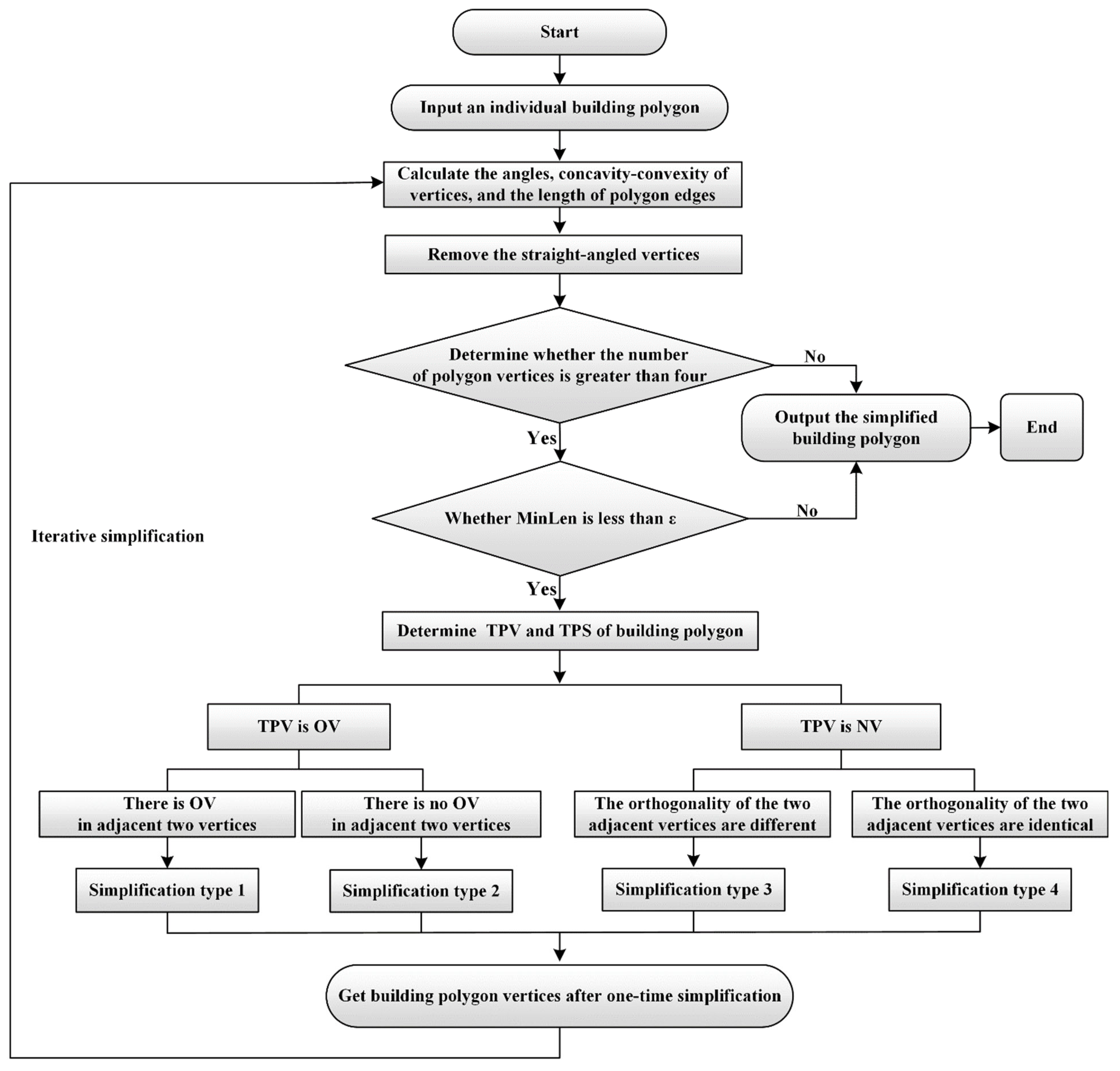
This study only discusses the simplification of the outer contour of buildings. According to the concavity–convexity and orthogonality of TPV and its two adjacent vertices, the types of simplification are classified, adopting different simplification algorithms. The minimum structure of a building polygon is simplified iteratively until it meets the requirement of simplification. The flowchart of simplification is shown in Figure 4.

Figure 4. The framework of our approach.

Step 1: Input the vertices of an individual building polygon. Calculate the angles, concavity–convexity of vertices, and the length of polygon edges.

Step 2: Remove the flat-angled vertices, that is, remove the redundant data.

Step 3: Determine whether the number of polygon vertices is greater than four. If it is more than four, go to step 4; otherwise, the polygon will not be simplified and its vertices will be output.

Step 4: Analyze whether $MinLen$ is less than $\epsilon$. If it is less than $\epsilon$, go to step 5; otherwise, the polygon will not be simplified and its vertices will be output.

Step 5: Determine the TPV and TPS of the building polygon.

Step 6: Determine the simplification type according to the orthogonality and concavity–convexity of the TPV and its adjacent two vertices. Then, perform the simplification with four simplification types: simplification types 1–4.

Step 7: Transfer the simplified building polygon to step 1 to perform iterative simplification until the building polygon meets the requirements of simplification.

3.5. Simplification Method

A building polygon can be represented by a set of vertices as $B_v=\left\{v_1,v_2,\cdots ,v_n\right\}$, and an edge set as $B_e=\left\{e\left(v_k,v_m\right)\right|v_k,v_m\in B_v\}$. Suppose $B_v$ should be simplified because the $MinLen$ is smaller than the threshold and $n>4$. The $TPV=\left\{v_i\right|v_i\in B_v\}$, $FAV=\left\{v_{i-1}\right|v_{i-1}\in B_v\}$, $RAV=\left\{v_{i+1}\right|v_{i+1}\in B_v\},$ then the TPS can be represented by $\{v_{i-1},v_i,v_{i+1}\}$. The four types of simplification method are the following:

3.5.1. Simplification Type 1: TPV Is OV, and there Is OV in Two Adjacent Vertices

This type usually belongs to regular polygons, which are common in buildings. In the simplification process, the areas of the filled parts are equal to that of the deleted parts to maintain the area of the building. Some local structure, e.g., the narrow and long concave (convex), should be exaggerated instead of deleting some details. The $StrA$ of TPV is used to determine whether to exaggerate. The threshold of the exaggerated $StrA$ of the TPV is denoted as $\gamma$. When $StrArea\ge \gamma$, the TPS will be exaggerated. According to the concavity and convexity of three vertices, there are 8 subtypes to be simplified:

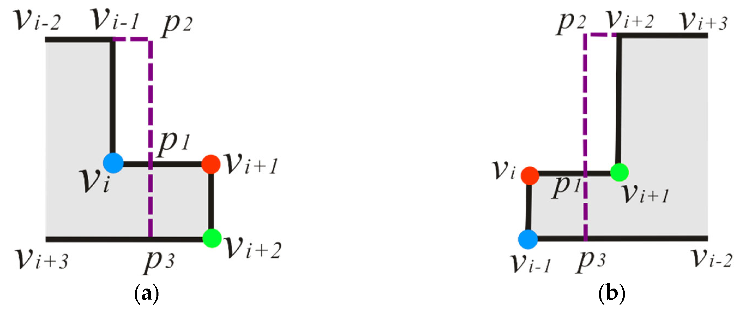
Subtype 1: $TPS\in \{FAV=CVV, TPV=CVV, RAV=CVV, StrA<\gamma \}$, as Figure 5a shows, draw a line $p_1{p}_2$ parallel to edge $e\left(v_i,v_{i+1}\right)$, in which $p_1$ is on $e\left(v_i,v_{i-1}\right)$, and $p_2$ is on $e\left(v_{i+1},v_{i+2}\right)$. Extend $p_2{p}_1$ and $v_{i-2}{v}_{i-1}$ to get an intersected point $p_3$. The area of quadrilateral $p_1{p}_2{v}_{i+1}{v}_i$ is equal to the triangle $p_1{p}_3{v}_{i-1}$. Then, the local structure $\{v_{i-2},v_{i-1},v_i,v_{i+1},v_{i+2}\}$ is simplified as $\{v_{i-2},p_3,p_2,v_{i+2}\}$.

Figure 5. The simplification subtypes 1–4 and their operations. (a) Subtype 1, (b) subtype 2, (c) subtype 3, (d) subtype 4.

Subtype 2: $TPS\in \{FAV=CCV, TPV=CCV, RAV=CCV, StrA<\gamma \}$, if $|v_i{v}_{i-1}\left|\le |v_i{v}_{i+1}\right|$, from $v_{i-1}$ draw a vertical line to edge $e\left(v_{i+1},v_{i+2}\right)$ at $p_1$. Then, the local structure $\{v_{i-2},v_{i-1},v_i,v_{i+1},v_{i+2}\}$ is simplified as $\{v_{i-2},v_{i-1},p_1,v_{i+2}\}$, as Figure 5b shows. If $\left|v_i{v}_{i-1}\right|>\left|v_i{v}_{i+1}\right|$, from $v_{i+1}$ draw a vertical line to edge $e\left(v_{i-1},v_{i-2}\right)$ at $p_1$. Then, the local structure $\{v_{i-2},v_{i-1},v_i,v_{i+1},v_{i+2}\}$ is simplified as $\{v_{i-2},p_1,v_{i+1},v_{i+2}\}$.

Subtype 3: $TPS\in \{FAV=CCV, TPV=CCV, RAV=CVV, StrA<\gamma \}$, as Figure 5c shows, draw a line $p_1{p}_3$ parallel to edge $e\left(v_{i-1},v_i\right)$, in which $p_1$ is on $e\left(v_i,v_{i+1}\right)$, and $p_3$ is on $e\left(v_{i-2},v_{i-1}\right)$. Draw a line $p_1{p}_2$ parallel to edge $e\left(v_{i+1},v_{i+2}\right)$, in which $p_2$ is on the line $v_{i+2}{v}_{i+3}$. The area of quadrilateral $p_1{p}_2{v}_{i+2}{v}_{i+1}$ is equal to the quadrilateral $p_1{p}_3{v}_{i-1}{v}_i$. Then, the local structure $\{v_{i-2},v_{i-1},v_i,v_{i+1},v_{i+2},v_{i+3}\}$ is simplified as $\{v_{i-2},p_3,p_1,p_2,v_{i+3}\}$.

Subtype 4: $TPS\in \{FAV=CVV, TPV=CCV, RAV=CCV, StrA<\gamma \}$, as Figure 5d shows, draw a line $p_1{p}_3$ parallel to edge $e\left(v_i,v_{i+1}\right)$, in which $p_1$ is on $e\left(v_i,v_{i-1}\right)$, and $p_3$ is on $e\left(v_{i+2},v_{i+1}\right)$. Draw a line $p_1{p}_2$ parallel to edge $e\left(v_{i-1},v_{i-2}\right)$, in which $p_2$ is on the line $v_{i-2}{v}_{i-3}$. The area of quadrilateral $p_1{p}_2{v}_{i-2}{v}_{i-1}$ is equal to the quadrilateral $p_1{p}_3{v}_{i+1}{v}_i$. Then, the local structure $\{v_{i-3},v_{i-2},v_{i-1},v_i,v_{i+1},v_{i+2}\}$ is simplified as $\{v_{i-3},p_2,p_1,p_3,v_{i+2}\}$. The simplification operation of subtype 3 corresponds to subtype 4 because of the difference in the concavity–convexity of FAV and RAV.

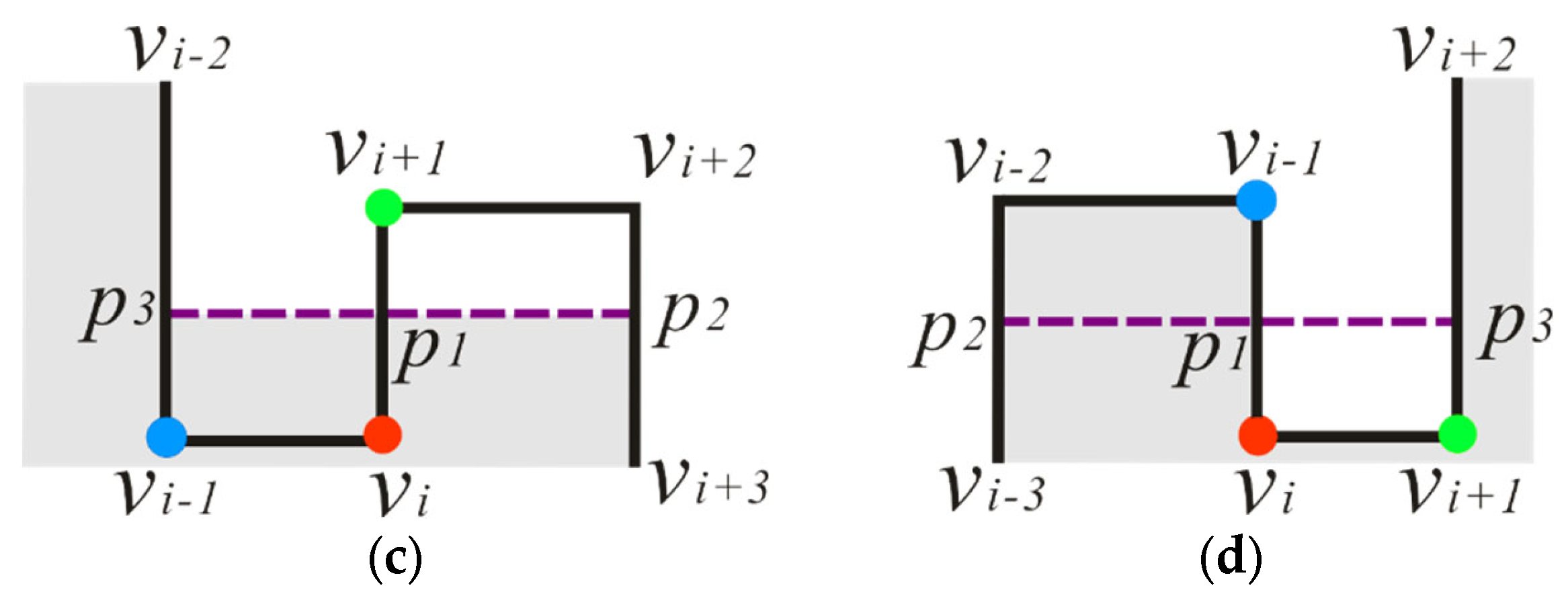
Subtype 5: $TPS\in \{FAV=CCV, TPV=CVV, RAV=CVV, StrA<\gamma \}$, as Figure 6a shows, draw a line $p_1{p}_3$ parallel to edge $e\left(v_{i+1},v_{i+2}\right)$, in which $p_1$ is on $e\left(v_i,v_{i+1}\right)$, and $p_3$ is on $e\left(v_{i+2},v_{i+3}\right)$. Draw a line $p_1{p}_2$ parallel to edge $e\left(v_i,v_{i-1}\right)$, in which $p_2$ is on the line $v_{i-2}{v}_{i-1}$. The area of quadrilateral $p_1{p}_2{v}_{i-1}{v}_i$ is equal to the quadrilateral $p_1{p}_3{v}_{i+2}{v}_{i+1}$. Then, the local structure $\left\{v_{i-2},v_{i-1},v_i,v_{i+1},v_{i+2},v_{i+3}\right\}$ is simplified as $\{v_{i-2},p_2,p_1,p_3,v_{i+3}\}$.

Figure 6. The simplification subtypes 5–8 and their operations. (a) Subtype 5, (b) subtype 6, (c) subtype 7, (d) subtype 8.

Subtype 6: $TPS\in \{FAV=CVV, TPV=CVV, RAV=CCV, StrA<\gamma \}$, as Figure 6b shows, draw a line $p_1{p}_3$ parallel to edge $e\left(v_i,v_{i-1}\right)$, in which $p_1$ is on $e\left(v_i,v_{i+1}\right)$, and $p_3$ is on $e\left(v_{i-1},v_{i-2}\right)$. Draw a line $p_1{p}_2$ parallel to edge $e\left(v_{i+1},v_{i+2}\right)$, in which $p_2$ is on the line $v_{i+3}{v}_{i+2}$. The area of quadrilateral $p_1{p}_2{v}_{i+2}{v}_{i+1}$ is equal to the quadrilateral $p_1{p}_3{v}_{i-1}{v}_i$. Then, the local structure $\left\{v_{i-2},v_{i-1},v_i,v_{i+1},v_{i+2},v_{i+3}\right\}$ is simplified as $\{v_{i-2},p_3,p_1,p_2,v_{i+3}\}$. The simplification operation of subtype 5 corresponds to subtype 6.

Subtype 7: $TPS\in \{FAV=CCV, TPV=CVV, RAV=CCV, StrA<\gamma \}$, as Figure 6c shows, draw a line $p_4{p}_5$ parallel to edge $e\left(v_{i-1},v_{i-2}\right)$, in which $p_4$ is on $e\left(v_i,v_{i-1}\right)$, and $p_5$ is on the line $v_{i-3}{v}_{i-2}$. Simultaneously, draw a line $p_2{p}_3$ parallel to edge $e\left(v_{i+1},v_{i+2}\right)$, in which $p_2$ is on $e\left(v_i,v_{i+1}\right)$, and $p_3$ is on the line $v_{i+3}{v}_{i+2}$. The line $p_4{p}_5$ intersects $p_2{p}_3$ at point $p_1$. The constraint is that the length ratio of $v_i{p}_4$ to $v_i{v}_{i-1}$ is equal to the length ratio of $v_i{p}_2$ to $v_i{v}_{i+1}$. Additionally, the area of quadrilateral $p_1{p}_2{v}_i{p}_4$ is equal to the sum of the area of quadrilaterals $p_4{p}_5{v}_{i-2}{v}_{i-1}$ and $p_2{p}_3{v}_{i+2}{v}_{i+1}$. Then, the local structure $\left\{v_{i-3},v_{i-2},v_{i-1},v_i,v_{i+1},v_{i+2},v_{i+3}\right\}$ is simplified as $\{v_{i-3},p_5,p_1,p_3,v_{i+3}\}$.

Subtype 8: $TPS\in \{FAV=CVV, TPV=CCV, RAV=CVV, StrA<\gamma \}$, as Figure 6d shows, the simplification operation of subtype 8 is the same as subtype 7, which is not repeated here.

Exaggeration types: If $TPS\in \left\{ StrA\ge \gamma \right\}$, the operation of exaggeration is performed. The length of shortest edge is extended to $\epsilon$ while preserving the area after exaggeration. According to the length of edge $e\left(v_i,v_{i-1}\right)$ and $e\left(v_i,v_{i+1}\right)$. There are two types: Exaggeration 1 and Exaggeration 2.

Exaggeration 1: If $\left|v_{i-1}{v}_i\right|<\left|v_i{v}_{i+1}\right|$, as Figure 7a shows, point $p_1$ is determined on the edge $e\left(v_i,v_{i+1}\right)$. Draw a line $p_1{p}_2$ parallel to edge $e\left(v_i,v_{i-1}\right)$, in which $p_2$ is on the line $v_{i-1}{v}_{i-2}$. Extend $p_2{p}_1$ to $p_3$ while $\left|p_2{p}_3\right|=\epsilon$. Draw a line $p_3{p}_4$ parallel to edge $e\left(v_i,v_{i+1}\right)$, in which $p_4$ is on the line $v_{i+1}{v}_{i+2}$. The area of quadrilateral $p_1{p}_2{v}_{i-1}{v}_i$ is equal to the quadrilateral $p_1{p}_3{p}_4{v}_{i+1}$. Then, the local structure $\left\{v_{i-2},v_{i-1},v_i,v_{i+1},v_{i+2}\right\}$ is simplified as $\{v_{i-2},p_2,p_3,p_4,v_{i+2}\}$.

Figure 7. The Exaggeration types and their operations: (a) Exaggeration 1, and (b) Exaggeration 2.

Exaggeration 2: If $\left|v_{i-1}{v}_i\right|>\left|v_i{v}_{i+1}\right|$, as Figure 7b shows, point $p_1$ is determined on the edge $e\left(v_i,v_{i-1}\right)$. Draw a line $p_1{p}_2$ parallel to edge $e\left(v_i,v_{i+1}\right)$, in which $p_2$ is on the line $v_{i+1}{v}_{i+2}$. Extend $p_2{p}_1$ to $p_3$ while $\left|p_2{p}_3\right|=\epsilon$. Draw a line $p_3{p}_4$ parallel to edge $e\left(v_i,v_{i-1}\right)$, in which $p_4$ is on the line $v_{i-1}{v}_{i-2}$. The area of quadrilateral $p_1{p}_2{v}_{i+1}{v}_i$ is equal to the quadrilateral $p_1{p}_3{p}_4{v}_{i-1}$. Then, the local structure $\left\{v_{i-2},v_{i-1},v_i,v_{i+1},v_{i+2}\right\}$ is simplified as $\{v_{i-2},p_4,p_3,p_2,v_{i+2}\}$.

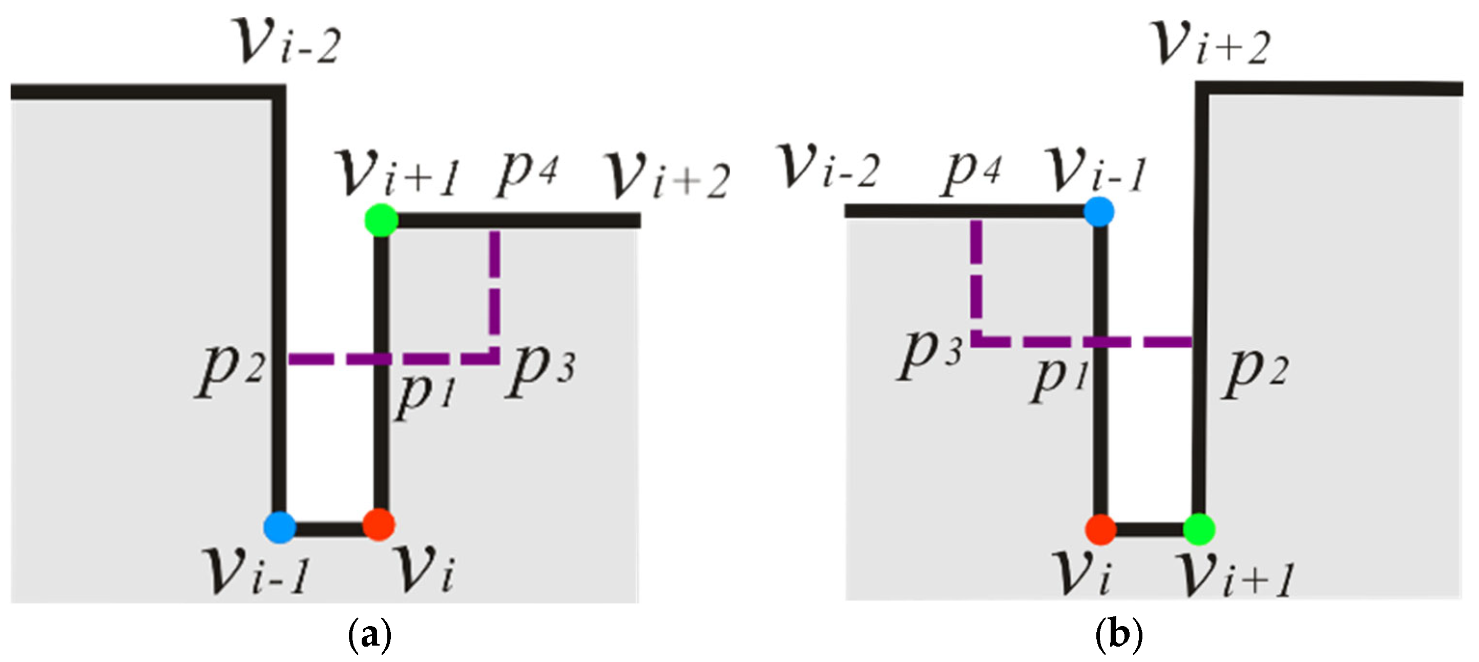
3.5.2. Simplification Type 2: TPV Is OV, and There Is No OV in Two Adjacent Vertices

Subtype 9: This simplification of the subtype is independent of convexity–concavity of TPV and its adjacent vertices. As Figure 8a shows, draw a line $p_1{p}_2$ parallel to $v_{i-1}{v}_{i+1}$, in which $p_1$ is on $e\left(v_i,v_{i+1}\right)$, and $p_2$ is on $e\left(v_{i-1},v_i\right)$. Prolong $p_1{p}_2$ and $p_2{p}_1$ to intersect $v_{i-2}{v}_{i-1}$ and $v_{i+1}{v}_{i+2}$ at $p_3$ and $p_4$, respectively. The area of the filled triangle $v_i{p}_1{p}_2$ is equal to the sum of area of the deleted triangles $v_{i-1}{p}_2{p}_3$ and $v_{i+1}{p}_1{p}_4$. Then, the local structure $\left\{v_{i-2},v_{i-1},v_i,v_{i+1},v_{i+2}\right\}$ is simplified as $\{v_{i-2},p_3,p_4,v_{i+2}\}$. In the special case that $v_{i-2}{v}_{i-1}$ and $v_{i+1}{v}_{i+2}$ are co-linear, $v_i$ is directly deleted. As Figure 8b shows, the local structure $\left\{v_{i-2},v_{i-1},v_i,v_{i+1},v_{i+2}\right\}$ is simplified as $\left\{v_{i-2},v_{i-1},v_{i+1},v_{i+2}\right\}$.

Figure 8. The simplification subtype 9 and its operations: (a) Subtype 9, and (b) is the case that $v_{i-2}{v}_{i-1}$ and $v_{i+1}{v}_{i+2}$ are co-linear.

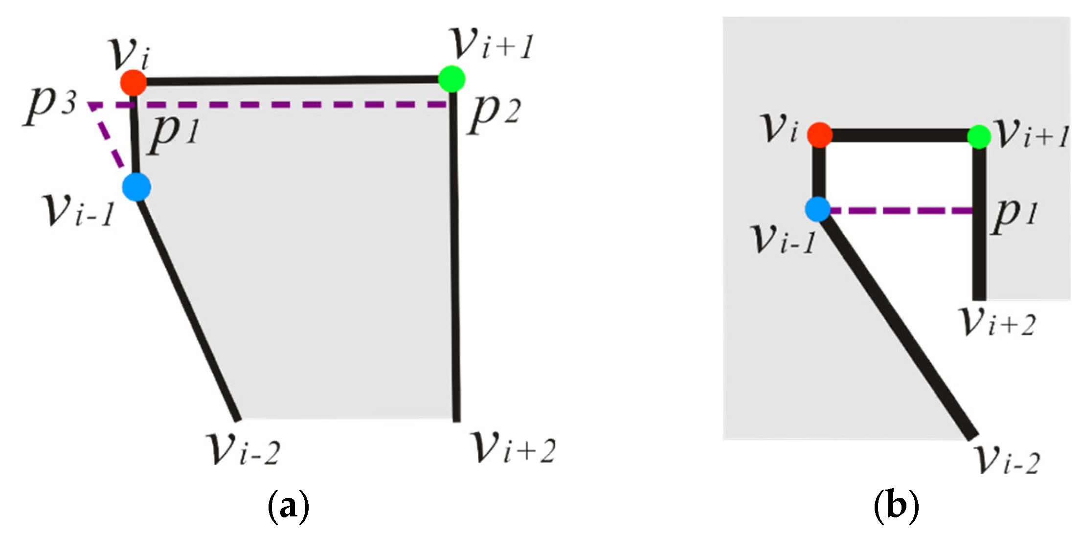
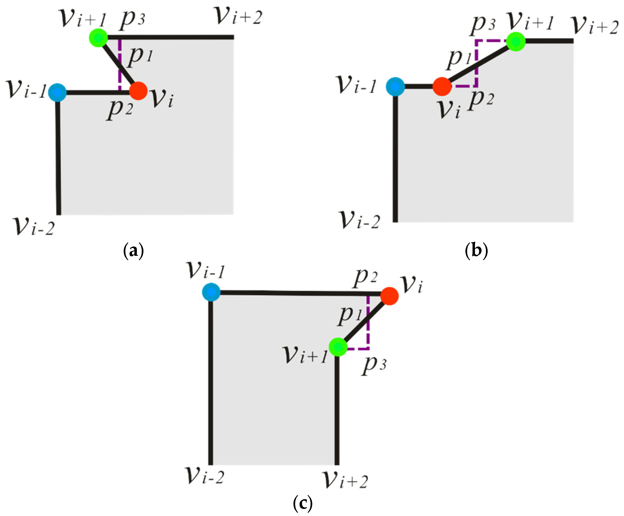
3.5.3. Simplification Type 3: TPV Is NV, and the Orthogonality of the Two Adjacent Vertices Is Different

Subtype 10: $TPS\in \left\{FAV=OV, TPV=NV, RAV=NV\right\}$. This simplification of the subtype is independent of convexity–concavity of TPV and its adjacent vertices. As Figure 9a–c shows, draw a line $p_1{p}_2$ perpendicular to $v_{i-1}{v}_i$, in which $p_1$ is on $e\left(v_i,v_{i+1}\right)$, and $p_2$ is on $e\left(v_{i-1},v_i\right)$. Denote the distance from $v_{i+1}$ to $e\left(v_{i-1},v_i\right)$ as $Dis$. Prolong $p_2{p}_1$ to $p_3$ while the length of $p_2{p}_3$ is $Dis$. The area of the triangle $v_i{p}_1{p}_2$ is equal to the triangle $v_{i+1}{p}_1{p}_3$. Then, the local structure $\left\{v_{i-2},v_{i-1},v_i,v_{i+1},v_{i+2}\right\}$ is simplified as $\{v_{i-2},v_{i-1},p_2,p_3,v_{i+1},v_{i+2}\}$. When $v_{i-1}{v}_i$ is parallel to $v_{i+1}{v}_{i+2}$, as Figure 9a,b shows, $p_3$, $v_{i+1}$, $v_{i+2}$ are collinear after simplification. $v_{i+1}$ is a flat-angled vertex, which will be deleted in the next iterative simplification process, see Section 3.4, Step 2 for details.

Figure 9. The simplification subtype 10 and its operations: (a–c) are different cases of subtype 10.

Subtype 11: $TPS\in \left\{FAV=NV, TPV=NV, RAV=OV\right\},$ the operation of simplification is similar to subtype 10, which will not be presented in detail here.

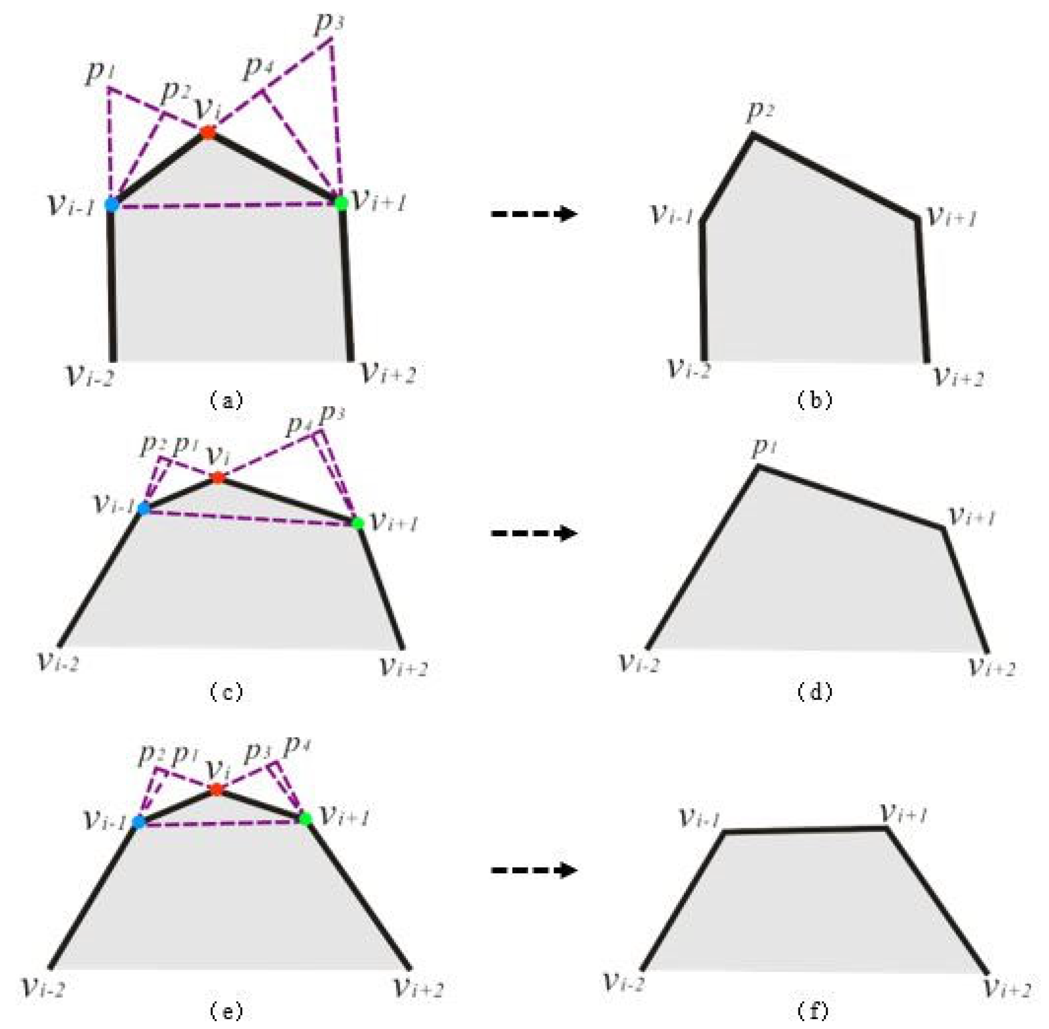
3.5.4. Simplification Type 4: TPV Is NV, and the Orthogonality of the Two Adjacent Vertices Is Identical

In this type, the shape and structure of the buildings are usually irregular. To preserve its characteristics and area as much as possible, an “Area-Comparison-Simplification-Method” is adopted herein. The idea is that the TPV is displaced to different positions, comparing the changes in area of the polygon after displacement. Then, the position with the smallest changes in the area is taken as the new position of the TPV. To preserve the shape features and right-angle of the building, the position of displacement is generally constructed by drawing perpendicular or intersectant lines.

Subtype 12: $TPS\in \left\{FAV=NV, TPV=NV, RAV=NV\right\}\cup \left\{FAV=OV, TPV=NV, RAV=OV\right\}$, as Figure 10 shows, draw $v_{i-1}{p}_2$, $v_{i+1}{p}_4$ perpendicular to $v_i{v}_{i+1}$ and $v_i{v}_{i-1}$, respectively, in which $p_2$ is on the line $v_i{v}_{i+1}$, and $p_4$ is on $v_{i-1}{v}_i$. Then, extend $v_{i-2}{v}_{i-1}$ and $v_{i+2}{v}_{i+1}$ intersect $v_{i+1}{v}_i$, $v_{i-1}{v}_i$ at $p_1$ and $p_3$, respectively. For $v_i$, which is the TPV, generally, five positions for displacement exist: $p_1$, $p_2$, $p_3$, $p_4$, and $v_{i+1}$ (that is, $v_i$ is deleted). When the constructed displacement position exists, the changing area corresponding to each displacement position is calculated. The changing area corresponding to $p_1$, which is denoted as $S_{p_{1 }}$, is the area of the triangle $v_{i-1}{v}_i{p}_1$. That is, $S_{p_1}=△v_{i-1}{v}_i{p}_1$. Similarly, the changed area corresponding to $p_2$, $p_3$, $p_4$ and $v_{i+1}$ is $S_{p_2}$, $S_{p_3}$, $S_{p_4}$, and $S_{v_{i+1}}$, respectively, where $S_{p_2}=△v_{i-1}{v}_i{p}_2$, $S_{p_3}=△v_i{v}_{i+1}{p}_3$, $S_{p_4}=△v_i{v}_{i+1}{p}_4$, and $S_{v_{i+1}}$ =$△v_{i-1}{v}_i{v}_{i+1}$.

Figure 10. The simplification subtype 12 and its operations: (a,c,e) are different local structures of subtype 12, and (b–f) are the simplified results correspondingly.

If $S_{p_2}$ is the smallest, as Figure 10a shows, $v_i$ is displaced to $p_2$. Then, the local structure $\left\{v_{i-2},v_{i-1},v_i,v_{i+1},v_{i+2}\right\}$ is simplified as $\{v_{i-2},v_{i-1},p_2,v_{i+1},v_{i+2}\}$, as shown in Figure 10b. The operation of $S_{p_4}$ is the same as $S_{p_2}$. If $S_{p_1}$ is the smallest, as Figure 10c shows, $v_i$ is displaced to $p_1$. Then, $\left\{v_{i-2},v_{i-1},v_i,v_{i+1},v_{i+2}\right\}$ is simplified as $\{v_{i-2},p_1,v_{i+1},v_{i+2}\}$, as shown in Figure 10d. The operation of $S_{p_3}$ is the same as $S_{p_1}$. If $S_{v_{i+1}}$ is the smallest, as Figure 10e shows, $v_i$ is deleted. Then, $\left\{v_{i-2},v_{i-1},v_i,v_{i+1},v_{i+2}\right\}$ is simplified as $\{v_{i-2},v_{i-1},v_{i+1},v_{i+2}\}$, shown in Figure 10f.

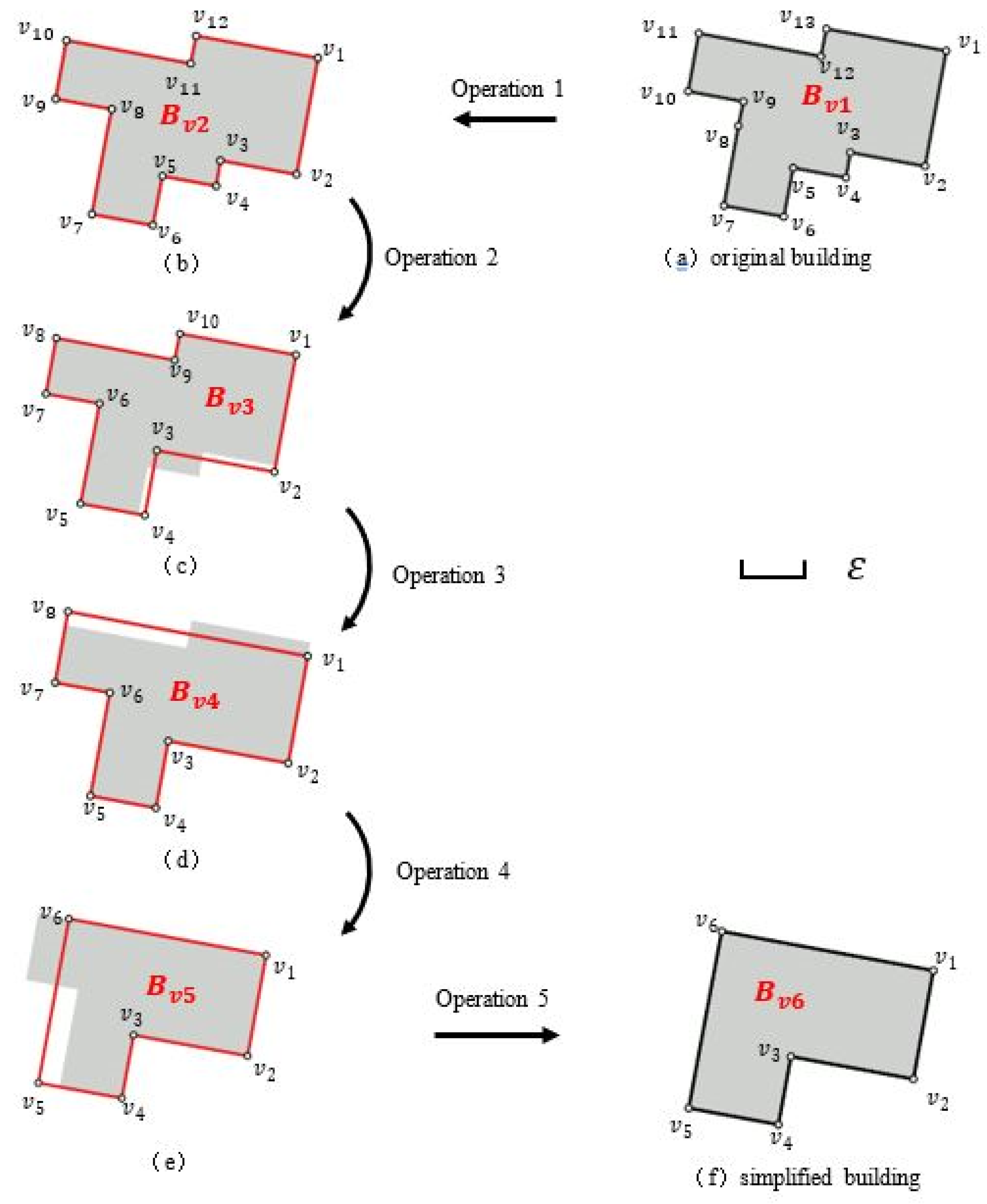
3.6. Example of the Simplification Process

To illustrate the simplification process, take the building $B_{v1}=\left\{v_1,v_2,\cdots ,v_{13}\right\}$ in the Figure 11a as an example. Suppose that, at the target scale, the minimum granularity is $\epsilon$. $\gamma ={\epsilon }^2$. To get the simplified building $B_{v6}=\left\{v_1,v_2,\cdots ,v_6\right\}$, there are five operations:

Figure 11. Example of the simplification process: (a) is the original building, (f) is the simplified building, and (b–e) are the process of simplification.

Operation 1: Take the $B_{v1}=\left\{v_1,v_2,\cdots ,v_{13}\right\}$ as the input. Calculate the angles, concavity–convexity of the vertices, and the length of polygon edges. Before each simplification operation, the flat-angled vertices (FV) are removed; thus, $v_8$ in $B_{v1}$ is removed. The building is presented as $B_{v2}=\left\{v_1,v_2,\cdots ,v_{12}\right\}$ in Figure 11b. The number of vertices in $B_{v2}$ is 12, which is greater than 4, and the $MinLen$ of $B_{v2}$ is less than $\epsilon$. Therefore, $B_{v2}$ should be simplified.

Operation 2: $B_{v2}$ is simplified to $B_{v3}$. First, determine $v_4$ in $B_{v2}$ as the TPV by finding the shortest edge $e\left(v_3,v_4\right)$ and comparing the structural area of $v_3,v_4$. Then, $FAV=v_3$, $RAV=v_5$, and the $TPS=\left\{v_3,v_4,v_5\right\}$. $TPS\in \left\{f_{ort}\left(TPV\right)=\mathrm{OV}, f_{ort}\left(FAV\right)=OV\cup f_{ort}\left(RAV\right)=OV\right\}$, which belongs to Simplification type 1. The structural area of $TPV$ is $Str{A}_4$, which is less than $\gamma$. As the concavity–convexity of $v_3,v_4,v_5$ is CCV, CVV, CCV, subtype 7 is adopted. The building is simplified as $B_{v3}=\left\{v_1,v_2,\cdots ,v_{10}\right\}$ in Figure 11c.

Operation 3: $B_{v3}$ is simplified to $B_{v4}$ iteratively. First, take $B_{v3}=\left\{v_1,v_2,\cdots ,v_{10}\right\}$ as the input to remove the FV, and there is no FV in $B_{v3}$. Then, as the $MinLen$ of $B_{v3}$ is less than $\epsilon$, $B_{v3}$ needs to be simplified continuously. In $B_{v3}$, $v_{10}$ is determined as the TPV, and the $TPS=\left\{v_9,v_{10},v_1\right\}$. $TPS\in \left\{f_{ort}\left(TPV\right)=\mathrm{OV}, f_{ort}\left(FAV\right)=OV\cup f_{ort}\left(RAV\right)=OV\right\}$, which belongs to Simplification type 1. As the concavity–convexity of $v_9,v_{10},v_1$ is CCV, CVV, CVV, subtype 5 is adopted. The building is simplified as $B_{v4}=\left\{v_1,v_2,\cdots ,v_8\right\}$ in Figure 11d.

Operation 4: $B_{v4}$ is simplified to $B_{v5}$ iteratively. First, take $B_{v4}=\left\{v_1,v_2,\cdots ,v_8\right\}$ as the input to remove the FV, and there is no FV in $B_{v4}$. Then, as the $MinLen$ of $B_{v4}$ is less than $\epsilon$, $B_{v4}$ needs to be simplified continuously. In $B_{v4}$, $v_7$ is determined as the TPV, and the $TPS=\left\{v_6,v_7,v_8\right\}$. $TPS\in \left\{f_{ort}\left(TPV\right)=\mathrm{OV}, f_{ort}\left(FAV\right)=OV\cup f_{ort}\left(RAV\right)=OV\right\}$, which belongs to Simplification type 1. As the concavity–convexity of $v_6,v_7,v_8$ is CCV, CVV, CVV, subtype 5 is adopted. The building is simplified as $B_{v5}=\left\{v_1,v_2,\cdots ,v_6\right\}$ in Figure 11e.

Operation 5: $B_{v5}$ is taken as the output. First, take $B_{v5}=\left\{v_1,v_2,\cdots ,v_6\right\}$ as the input to remove the FV, and there is no FV in $B_{v5}$. Then, as the $MinLen$ of $B_{v5}$ is more than $\epsilon$, the simplification meets the constraint. Therefore, take $B_{v5}=\left\{v_1,v_2,\cdots ,v_6\right\}$ as the result of the simplification for $B_{v1}=\left\{v_1,v_2,\cdots ,v_{13}\right\}$, as Figure 11f shows.

Moreover, if a smaller detail of outlines is generated in the Simplification types, it will be eliminated in the iterative simplification process.

4. Experiment and Analysis

4.1. Determination of the Simplification Evaluation Indicators

To evaluate the feasibility and adaptability of our method, the change in the number of vertices ($NumC$), the change in the area ($AreaC$), the change in ratio of orthogonal vertices ($OrtC$), the change in position of the center point ($CtrPC$), the change in shape in global ($SGC$), and the change in shape in details ($SDC$) [8,41] are selected as the evaluation indicators, which are defined as the following:

Suppose an original building is presented as $B_{ori}=\left\{v_1,v_2,\cdots ,v_n\right\}$ before simplification. The area of $B_{ori}$ is $Are{a}_{ori}$, the center point of $B_{ori}$ is $C{P}_{ori}$, and the number of orthogonal vertices in $B_{ori}$ is $n_{ov}$. The simplified building is presented as $B_{sim}=\left\{v_1^{,},v_2^{,},\cdots ,v_m^{,}\right\}$. The area of $B_{sim}$ is $Are{a}_{sim}$, the center point of $B_{sim}$ is $C{P}_{sim}$, and the number of orthogonal vertices in $B_{sim}$ is $m_{ov}$. ($x_0,y_0$) and ($x_s,y_s$) are the coordinates of $C{P}_{ori}$ and $C{P}_{sim}$.

$$NumC=\left(m-n\right)/n, NumC\in \left[-1,0\right]$$

(6)

$$AreaC=|\frac{Are{a}_{sim}-Are{a}_{ori}}{Are{a}_{ori}}|, AreaC\in \left[0,\infty \right]$$

(7)

$$OrtC=\left(\frac{m_{ov}}{m}-\frac{n_{ov}}{n}\right)\times 100\%, OrtC\in \left[-1,1\right]$$

(8)

$$CtrPC=\sqrt{{\left(x_0-x_s\right)}^2+{\left(y_0-y_s\right)}^2}, CtrPC\in \left[0,\infty \right]$$

(9)

$$SGC=Area\left(B_{ori}\cap B_{sim}\right)/Area\left(B_{ori}\cup B_{sim}\right), SGC\in \left[0,1\right]$$

(10)

where $NumC$ denotes whether the number of vertices is effectively reduced after simplification. $AreaC$ is an index to measure the conservation of area. $OrtC$ represents whether orthogonal features remain. $CtrPC$ shows the displaced distance of the building. $SGC$ denotes the change in shape of a building globally before and after simplification. Correspondingly, in order to compare the changes in the shape of buildings more specifically, $SGC$ is adopted.

As the building outlines have few vertices and right angles, it is suitable to measure the shape similarity of buildings in detail by adopting the turning function [48]. For a building, as Figure 12a shows, the tangent angle of an arbitrary point $O$ on its outline along a reference orientation (e.g., X-axis) is $\psi$, and the turning function $f\left(s\right)$ is defined as the change relationship of the tangent angle $\psi$ along its outline in a counterclockwise direction with respect to the arc length $s$ (as Figure 12b shows). The total arc length $s$ is 1 [42].

Figure 12. Definition of the turning function: (a) shows the tangent angle $\psi$, and (b) presents the turning function.

The $SDC$ between the original and simplified buildings is measured as follows [40]:

$$SDC=\frac{1}{2\pi }\sqrt{\underset{\varphi \in R, t\in \left[-1,1\right]}{\min }{{\displaystyle \int }}_0^1{\left[f_{ori}\left(s+t\right)-f_{sim}\left(s\right)+\varphi \right]}^{2}ds}$$

(11)

where $f_{ori}\left(s\right)$ and $f_{sim}\left(s\right)$ are the turning functions of the original and simplified buildings, respectively, t denotes the distance over which the starting point (point $p$ in Figure 12a) moves along the outline, and $\varphi$ represents the rotation angle. Two buildings are more similar in shape the smaller the value of $SDC$ [15].

4.2. Experiments

Our method was tested and verified on ArcEngine 10.2 (ESRI, RedLands, CA, USA) using C#. Topographic building data with 540 buildings in the Netherlands, which is open data in the Kadaster, was used for our experiments (seen in Figure 13). The scale of original buildings data is 1:1000. At the scale of 1:25,000 ($\epsilon$ = 7.5 m), 540 buildings in a certain region of the Netherlands were simplified. The simplification results are shown in Figure 13a (gray shadow is the original shape of the building and red lines are simplified outlines). The time complexity of our approach is T(n) for simplifying a building, then O(n) ≤ T(n) ≤ O(n²), n is the number of vertices of a building.

Figure 13. Simplification of buildings at scale 1:25,000: (a) simplified result in a clear view, and (b,c) are the enlarged views.

With respect to various buildings with different shapes in cities, the proposed method has a good universality. On the whole, the simplification results keep a normal building shape, with no abnormal simplification, which shows that the algorithm has good adaptability to various types of buildings. From the locally enlarged view, as shown in Figure 13b,c, simplification can effectively reduce the local details of buildings, keeping the main shape of buildings, which conform to human habits of visual perception. The evaluation indicators of the simplified result are shown in Table 3. The average $AreaC$ is 0.41%, which indicates that our method could retain the area before and after simplification. The average $OrtC$ increased by 2.91%. The proposed method keeps the visual center of the buildings almost unchanged which is proved by average $CtrPC$ (0.3878 m). The value of $SGC$ could detect buildings with simplified anomalies. The percent of $SGC\ge 0.5$ is 99.81%, which means the simplified buildings preserve their shape. The only one building with $SGC$ < 0.5 is found, as the black arrow shows in Figure 13a, which was simplified to a satisfying rectangle. However, the simplification of 540 buildings takes 25.53 s, which has little advantage in terms of time efficiency.

Table 3. Evaluation indicators of the simplified result at scale 1:25,000.

Scale	$\mathbf{Average} \mathit{N}\mathit{u}\mathit{m}\mathit{C}$	$\mathbf{Average} \mathit{A}\mathit{r}\mathit{e}\mathit{a}\mathit{C}$	$\mathbf{Average} \mathit{O}\mathit{r}\mathit{t}\mathit{C}$	$\mathbf{Average} \mathit{C}\mathit{t}\mathit{r}\mathit{P}\mathit{C} \left(\mathbf{m}\right)$	$\mathit{S}\mathit{G}\mathit{C} > 0.5$	$\mathbf{Average} \mathit{S}\mathit{D}\mathit{C}$	Running Time (s)
1:25,000	−28.42%	0.41%	2.91%	0.3878	99.81%	0.0622	25.53

4.3. Multi-Scale Simplification

Our approach is useful for continuous scale transformation of buildings. For a given target scale ($Scal{e}^j$), a building ($B_i$) has a simplified representation ($B_i^j$) corresponding to the scale. As Figure 14 shows, 6 buildings with complex shape are selected from 540 buildings in Figure 13, which are denoted as $\{B_1,B_2,\cdots ,B_6\}$. $Scale=\left\{1000, \mathrm{10,000}, \mathrm{12,500}, \mathrm{15,000}, \mathrm{20,000}, \mathrm{22,500}, \mathrm{25,000}\right\}$. According to the target scale, each building has a representation.

Figure 14. Multi-scale simplification of buildings.

As shown in Figure 14, the simplification method proposed herein gradually simplifies the outline and local details of buildings with reducing scale, which reflects the progressive and multi-scale expression of simplification. We can realize the process by adjusting scales to determine the minimum granularity. As $B_1^1$ transforms to $B_1^7$, the minimal and unimportant details are deleted preferentially. The complex-shaped buildings are simplified to a simple one, which also preserves the main shape characteristics, e.g., $B_1^7$. Since the orthogonal characteristic of buildings is preserved well in continuous scale transformation, the results show that the proposed method simplifies rectangular buildings commendably, such as $B_2^1$ and $B_6^1$ in Figure 14. In addition, our method could keep the area of buildings before and after simplification by comparing the simplified outlines and original buildings at a scale of 25,000 in Figure 14, instead of simply removing vertices. Therefore, the proposed method has advantages in keeping the simplification result stable and controllable in continuous scale transformation of buildings.

4.4. Simplification Test of Typical Buildings

In order to evaluate the different behavior of the method on the shapes of typical buildings, we selected some typical buildings (the vertices of the building polygon are arranged clockwise) for the simplification test, including regular buildings and irregular buildings, as shown in Figure 15a.

Figure 15. Tests of building simplification. (a) is the original buildings and simplified result; (b) is the test of directional dependence; (c) is the test of changing vertices sequence as counterclockwise; (d,e) is the test of extrusion and stretching; (f) is the test of adjusting the start vertex.

① Test of directional dependence. Rotate the buildings with rotation angles $\omega$ of 90° in Figure 15b. From the simplification results, the simplification results of buildings in different angles are consistent, which confirms that the proposed method does not depend on the direction of buildings. ② Test of changing vertices sequence as counterclockwise, as Figure 15c shows. The simplification result 3 is the same as simplification result 1, confirming that our method provides the same output for the buildings encoded clockwise and counterclockwise. ③ Test of extrusion and stretching. In simplification, buildings may be stretched and extruded to different degrees. The buildings in Figure 15d,e, are obtained by extruding and stretching the buildings in Figure 15a, respectively. By comparison of simplification results 1, 4, and 5, the results of simplification are similar, with some local differences. It shows that this algorithm can simplify according to the shapes of different buildings, keeping the original shape characteristics of buildings in general. ④ Test of adjusting the start vertex. The buildings in Figure 15f are acquired by changing the start vertices of buildings in Figure 15a. The start vertices are denoted as red points in Figure 15f. Simplification result 6 is the same as simplification result 1, which confirms that the changing the sequence of vertices has no effect on the simplification result.

4.5. Method Comparison

The method proposed herein was compared to the adjacent four-point simplification method [15], local-structure-classification simplification method [8], ArcGIS 10.2 building simplification tool (Simplify Building), and recursive method [25] by simplifying 1594 buildings at scales of 1:25,000 ($\epsilon$ = 7.5 m), 1:50,000 ($\epsilon$ = 15 m), and 1:75,000 ($\epsilon$ = 22.5 m). The original scale of those buildings is 1:1000. Similar to the proposed method, the adjacent four-point simplification method also presented a processing of local structures. The local-structure-classification simplification method is a combined building simplification approach based on the local structure classification and backtracking strategy. ArcGIS is a well-rounded commercial software. The principle of the simplified method based on ArcGIS is removing unnecessary detail, such as extraneous bends and fluctuations, from a line or an area boundary without destroying its essential shape [49]. The recursive method is a traditional simplification approach which uses the least squares method.

In order to present the simplification effects of each method, we selected 85 typical buildings with complex shapes and different structural characteristics from simplified results, as Figure 16 shows, including circular-shaped buildings. Figure 17 was obtained by counting the six evaluation indicators of simplified buildings at different simplification thresholds.

Figure 16. Results of the comparison test.

Figure 17. Comparison of simplification methods at different thresholds: (a) NumC, (b) AreaC, (c) OrtC, (d) CtrPC, (e) SGC, (f) SDC.

Figure 16 shows that all the methods of simplification preserve the basic shape features of buildings and have an effective consequence on conventional buildings. However, the comparison of simplification effects shows that when the span of simplification scale is large, that is, when the simplification threshold is significantly larger than the length of edges in buildings, the proposed method is more suitable for the original outlines of the buildings and the simplification result is more stable compared to the existing methods. In the adjacent four-point method, the shape features are obviously changed due to sharpening, as shown by the blue arrow in Figure 16b. Individual buildings have some change in the shape in the local-structure-classification simplification method, as shown by the blue arrow in Figure 16c. The ArcGIS-based building simplification method fails to consider the area of some complex buildings during simplification. Moreover, the short edges of some buildings are not eliminated when $\epsilon$ = 22.5 m, as shown by the blue arrow in Figure 16d. The simplification result of the recursive method does not fit well with the shape of the original buildings. Because the recursive method determines the rotation angles according to the minimum bounding rectangle (MBR) of buildings, this leads to the direction deviation for some complex buildings, as shown by the blue arrow in Figure 16e. The buildings that are shown by the blue rectangles in Figure 16 are circular-shaped buildings. The proposed method maintains the circular-shaped characteristics in comparison with other methods. Specifically, the local-structure-classification simplification method fails to simplify some circular-shaped buildings. The ArcGIS-based method could keep the circular shape as a whole. However, some small structures are not simplified in the ArcGIS-based method. The adjacent four-point method and recursive method have comparatively large changes in shape characteristics for circular-shaped buildings.

The comparison of the simplified data (Figure 17a) shows that the rate of change in the number of vertices of the proposed method is close to the adjacent four-point method and recursive simplification method. As shown in Figure 17b, since the proposed method minimizes the change in the area of each simplification type as much as possible, the proposed method has certain advantages over the other four methods in terms of area preservation. According to the experimental data, the average rate of change in the area of the proposed method is 0.0142%, compared with 10.78% for the existing methods. In Figure 1c, the proposed algorithm effectively keeps the right-angled characteristic with the simplification threshold increasing. Because of the rectangular shape of buildings, the recursive method could maintain the orthogonality characteristics of buildings completely. Additionally, the displacement distance of the building center in the proposed method is smaller than other methods, as Figure 17d shows. The proposed method also has advantages in maintaining the main shape characteristics, which can be proved in Figure 17e,f. However, the simplification of “island-shaped” buildings is not studied in the proposed algorithm. Additionally, building simplification depending on contextual information is not involved.

5. Conclusions

The simplification of buildings is a classic problem in map generalization. We proposed a progressive simplification method for buildings, considering the preservation of shapes, orthogonality, and area for buildings at the same time. In our approach, the TPS and TPV are defined which transform the problem of building simplification into an iterative simplification of the minimum structure of buildings. According to the concave–convexity and orthogonality, the local structure TPS is classified into 62 types, which could cover all structures in the buildings. The simplification algorithm not only meets the requirements of map visualization, but also maintains the orthogonality and area as much as possible.

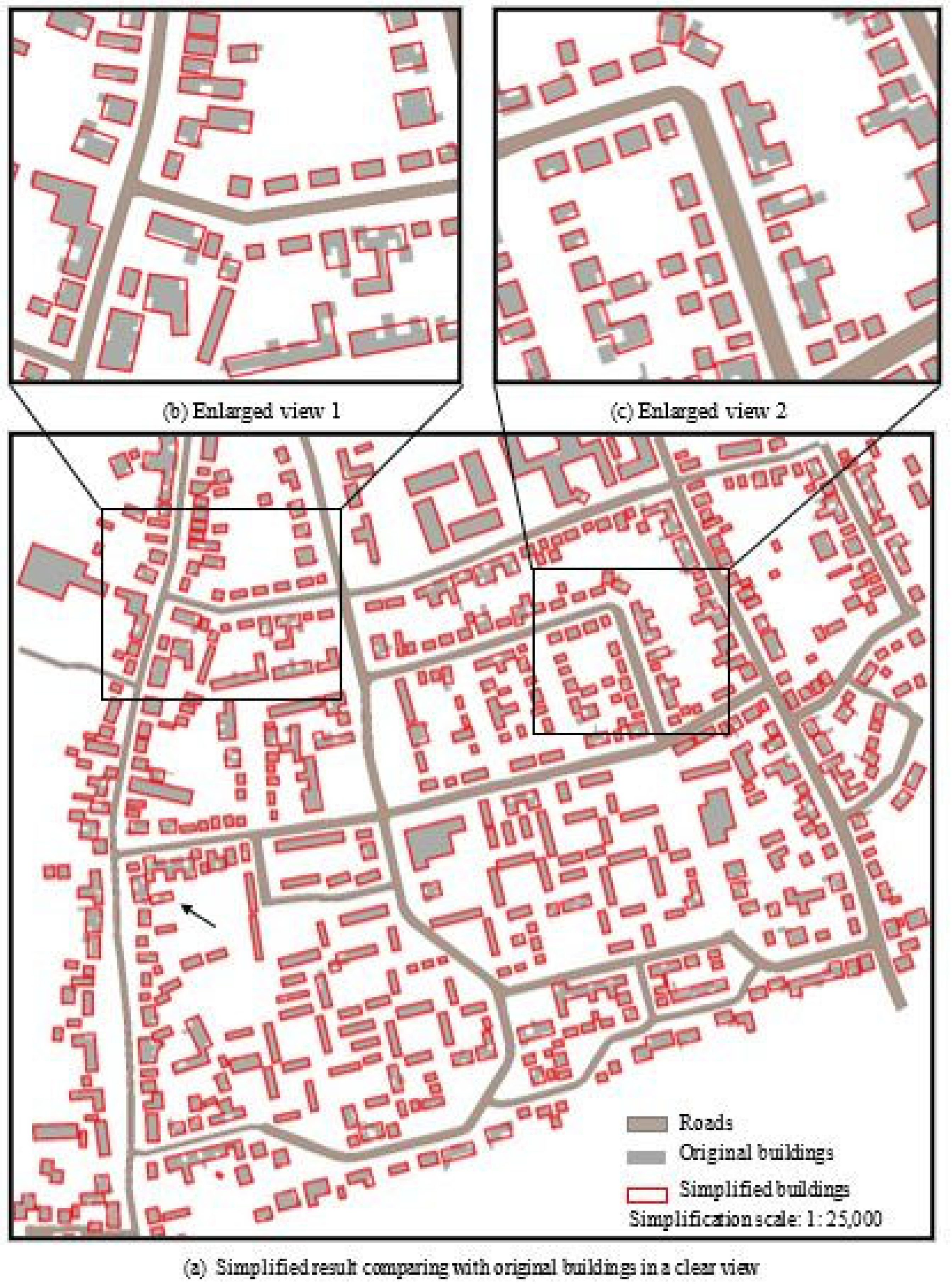
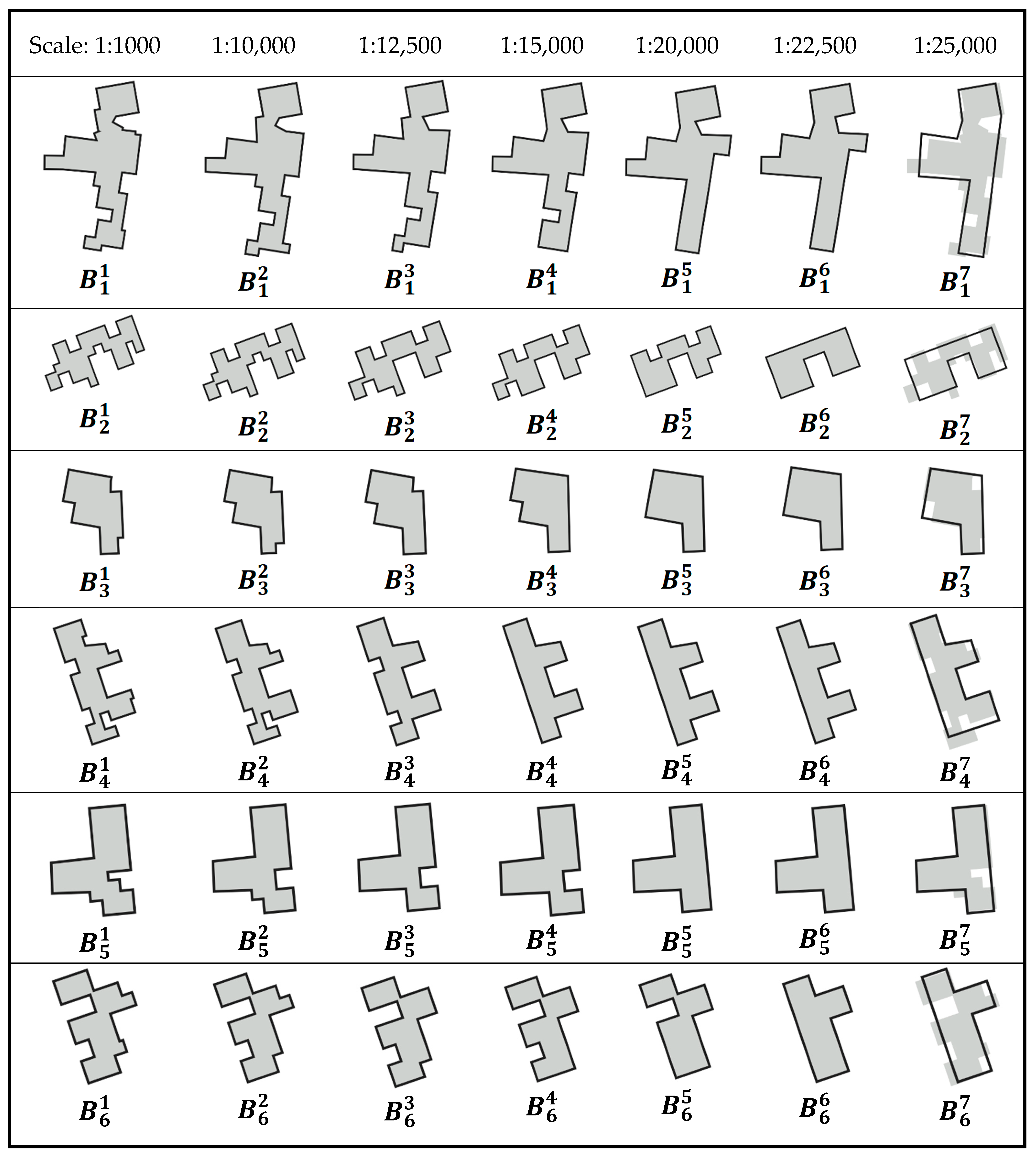
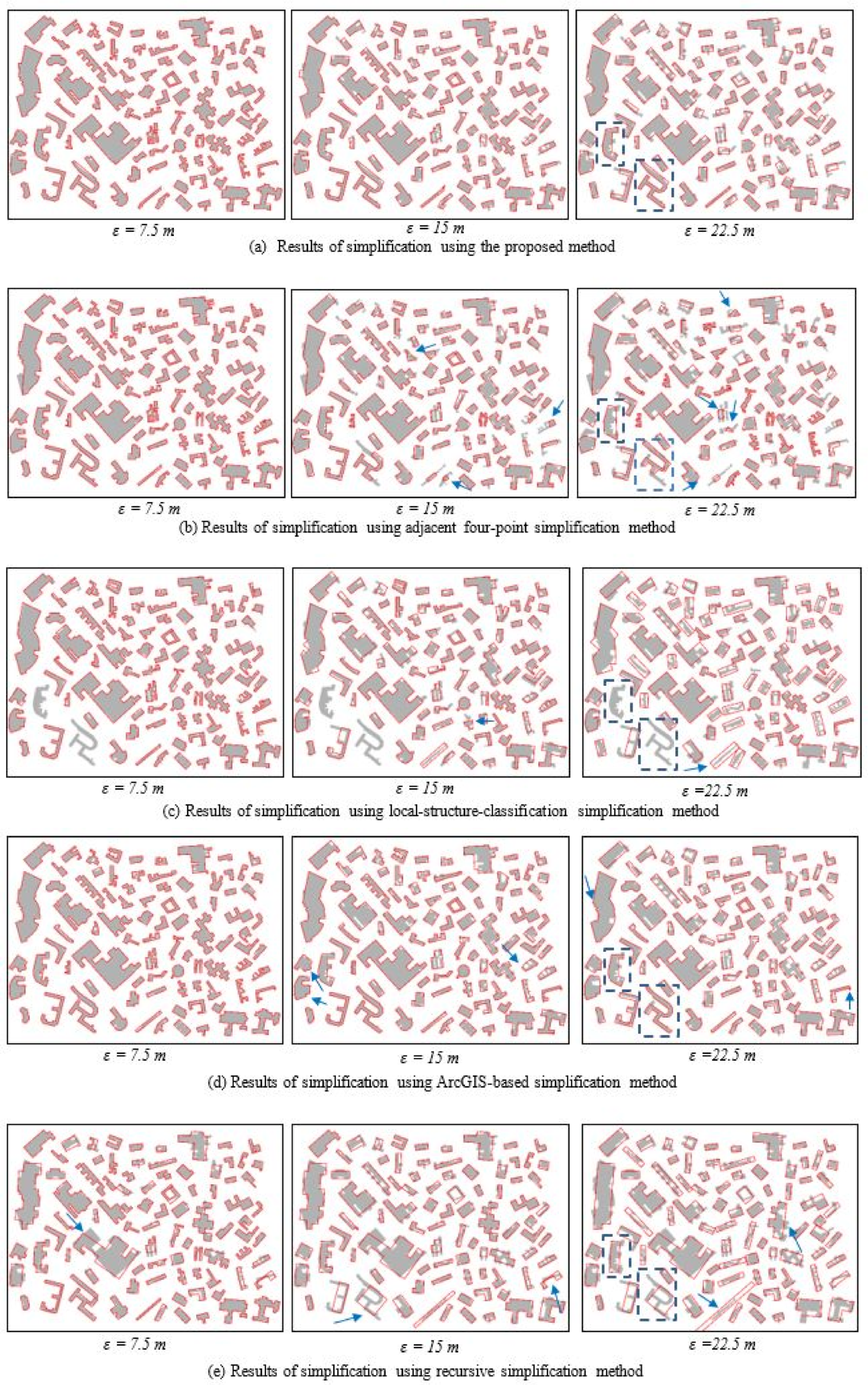
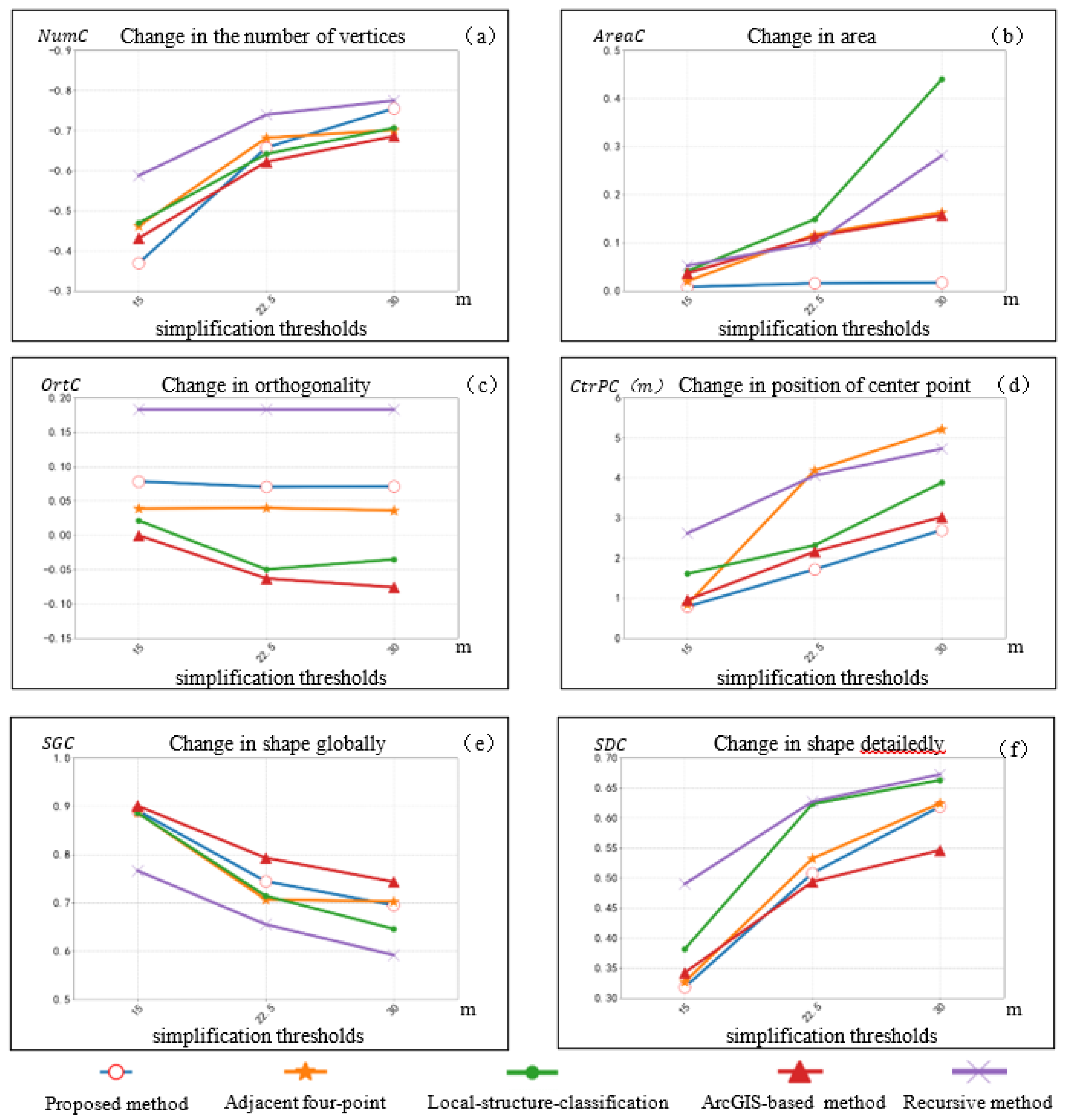
To verify the proposed method, some experiments were performed, including tests of multi-scale simplification, and typical buildings. The results of simplification indicate that our method is suitable for the multi-scale simplification of buildings, which is independent of the direction and vertices sequence of buildings. At multiple scales, buildings are simplified in accordance with the simplification rules. Compared to the adjacent four-point simplification method, local-structure-classification simplification method, ArcGIS-based building simplification method, and recursive method, the proposed method better preserves the shapes, orthogonality, and area of buildings, with minimal displacement of the center point. However, we only discuss the simplification of building outlines, which is just one kind of operation in map generalization. The proposed method needs to be combined with other generalization operations to achieve a reasonable result in the future, e.g., aggregation. Moreover, future research should include the following: (1) the collaborative simplification of the internal and external outlines of “island-shaped” buildings, and three-dimensional polygon simplification will be studied based on TPS; and (2) the influence of regional geographical features on building simplification will be considered to realize the composite simplification considering multiple features, not just individual buildings.