Generation Method for Shaded Relief Based on Conditional Generative Adversarial Nets

Abstract

Relief shading is the primary method for effectively representing three-dimensional terrain on a two-dimensional plane. Despite its expressiveness, manual relief shading is difficult and time-consuming. In contrast, although analytical relief shading is fast and efficient, the visual effect is quite different from that of manual relief shading due to the low degree of terrain generalisation, inability to adjust local illumination, and difficulty in exaggerating and selective representation. We introduce deep learning technology to propose a generation method for shaded relief based on conditional generative adversarial nets. This method takes the set of manual relief shading-digital elevation model (DEM) slices as a priori knowledge, optimises network parameters through a continuous game of “generation-discrimination”, and produces a shaded relief map of any region based on the DEM. Test results indicate that the proposed method retains the advantages of manual relief shading and can quickly generate shaded relief with quality and artistic style similar to those of manual shading. Compared with other networks, the shaded relief generated by the proposed method not only depicts the terrain clearly but also achieves a good generalisation effect. Moreover, through the use of an adversarial structure, the network demonstrates stronger cross-scale generation ability.

1. Introduction

The relief shading method summarises the distribution of light and shadow on the ground, using the shades of different tones on the map plane to represent changes in light and shadow so as to represent the terrain on a two-dimensional plane [1]. Compared with other methods that represent the depicted terrain on a plane, the terrain represented by relief shading shows a strong sense of three-dimensionality. This allows map readers to quickly grasp the terrain information.

At present, shaded relief can be generated quickly by many software packages, including ArcGIS (https://www.esri.com/, accessed on 15 May 2022), QGIS (https://www.qgis.org/, accessed on 15 May 2022), and Global Mapper (https://www.bluemarblegeo.com/, accessed on 15 May 2022). This form of software-generated shaded relief is termed analytical relief shading. Despite the advantages of a short production cycle and low requirements for operator effort, analytical relief shading has obvious shortcomings compared with manual relief shading. More specifically, in the generation of analytical shaded relief, the computer cannot fully consider the overall and local conditions of the mapped area. Instead, the computer provides a certain grey value, calculated strictly according to the light-receiving amount of each pixel in the digital elevation model (DEM). Although the grey value is calculated based on scientific knowledge, this method fails to generalise the broken terrain and flexibly adjust the azimuth and inclination of the illumination vector for the terrain in the local area, nor can this methodology exaggerate and selectively represent local areas. This results in a lack of expressiveness. When drawing relief shading manually, expert cartographers first delineate ridge and gully lines, then start shading along the main drainage divides. Additional details are added gradually, adjusting the direction of illumination and modulating the brightness of individual terrain forms to visually accentuate the main terrain structures and improve the representation of landforms. However, producing high-quality manual relief shading requires expert drawing skills and an extensive amount of time. These superb drawing skills are based on in-depth analysis and learned thought patterns of cartographers of the terrain, which can hardly be described accurately by mathematical models.

However, deep learning methods have significant advantages in solving problems that are difficult to describe with mathematical models, including with regard to object detection [2], image classification [3], and semantic segmentation [4]. If deep learning methods can be used to learn techniques such as terrain generalisation and local illumination adjustment from high-quality manual relief shading, the advantages of analytical relief shading and manual relief shading can be combined. Generative adversarial net (GAN) [5] is a deep learning model that has been widely applied in many fields. Due to the lack of constraints in GAN, the generated images are not strictly controlled. Mirza et al. thus proposed the concept of conditional generative adversarial nets (cGANs) [6]. Relief shading using a DEM can be seen as converting the input image to an output image, and cGANs are very suitable for solving this kind of problem [7].

In this paper, we propose a new method for generating relief shading. Based on cGAN and manual relief shading-DEM slice pairs, this method turns the problem of high-quality shaded relief generation into a problem of image-to-image translation. Firstly, the data is pre-processed, and the manual relief shading and DEM slices are segmented to create the training dataset. The cGAN that converts DEM into shaded relief is then established and trained using manual relief shading-DEM slice pairs. The trained network is eventually used to convert the DEM of any area into shaded relief.

The following sections of this paper cover the contents of our methodologic presentation as follows: Section 2 introduces related work conducted by researchers to optimise the effect of relief shading; Section 3 introduces the generation method for shaded relief based on cGAN; Section 4 determines the hyperparameters of the cGAN through testing and compares the network shading described herein with analytical relief shading, manual relief shading, and relief shading generated by other networks; and Section 5 summarises the conclusions drawn in this paper and discusses future work.

2. Related Work

There are two main issues that cause the inferior expressiveness of analytical relief shading as compared with manual relief shading. When manually drawing shaded relief, cartographers fully grasp the overall terrain of the mapped area and determine the main features thereof to carry out the cartographic generalisation. In the manual relief shading process, unimportant terrain details are ignored, and small hills are combined, integrated, exaggerated, or selectively represented. In contrast, relief shading based on software packages strictly presents all details of the DEM data according to the calculation model, resulting in an excessive amount of broken terrain details in the shaded relief; this prevents the readers from quickly understanding the terrain elements. As such, researchers have studied DEM generalisation algorithms to remove undesirable roughness; these methodologies evaluate the importance of each DEM pixel and select only the important pixels to reconstruct the DEM [8], extract topographic structure lines to analyse the spatial relationships between topographic features and topographic elements, and generalise a DEM with these topographic structure lines as constraints [9,10,11,12]. These algorithms regard a DEM as a digital image and use image processing techniques such as wavelet analysis [13] and image filtering [14] together with information theory [15] and terrain structure analysis [16] to simplify the DEM.

Moreover, during the generation of analytical shading, illumination is fixed and cannot be adjusted flexibly. As a result, when there are multiple ridges with different strikes, those in the same direction as the illumination are not easily identified. In contrast, manual relief shading adjusts the direction and intensity of illumination according to the local terrain, making the main terrain more obvious while also allowing some smaller but important terrains to be identified quickly [17]. The effect of illumination adjustment is shown in Figure 1. In view of this issue, many researchers have conducted in-depth studies, including adjusting local illumination using an interactive method [18]; adjusting illumination based on the direction of terrain feature lines [19], elevation and slope [20], and surface orientation [21]; adopting new illumination models (e.g., sky models) [22]; combining multiple shaded relief with different illumination directions [23] or combining shaded relief with a profile curvature map (one of the second derivatives of DEM) [24]; and adjusting pixel values according to the grey values at the terrain edges [11] and the multidirectional visibility index [25].

Although the above attempts have improved the relief shading effect to a certain extent, a gap still persists when compared with high-quality manual relief shading. For example, in terms of DEM generalisation, the process is complicated and the results are not satisfactory due to large information loss. Moreover, in terms of illumination, existing methods fail to improve expressiveness while reducing human manipulation. In sum, the above studies failed to meaningfully improve the relief shading effect, ultimately due to the fact that terrain generalisation and illumination adjustment require a full understanding of the mapped area (i.e., knowledge available to cartographers), and their implementation requires an abstract thinking process that can hardly be simulated by mathematical models.

However, deep learning technology allows a computational model composed of multiple processing layers to learn the representations of abstract data [26]. This has been applied by researchers in an attempt to improve the relief shading effect. For example, Patterson [27] introduced neural style transfer into relief shading, which successfully enhanced the expressiveness and artistic sense of the shaded relief. However, the terrain elements were distorted, were missed in some cases, and were generated where they did not exist in other cases. As another example, Jenny et al. [28] applied a neural network to the generation of relief shading and achieved pioneering results; the structure of U-Net [29] was improved and trained using manual relief shading. As the trained network follows the design principles of manual relief shading when rendering shaded relief imagery, the expressiveness of the generated shaded relief was greatly enhanced; these results are recognised by many expert cartographers. Nevertheless, the flat areas and sharp ridges generated in the shaded relief sometimes become blurred, and the network also performs poorly if the cell size of the DEM differs greatly from that used for network training. Since deep learning methods have been proven to greatly enhance the relief shading effect, many other deep learning networks are expected to hold the key to solving the existing issues noted above so as to further enhance the relief shading effect.

3. Materials and Methods

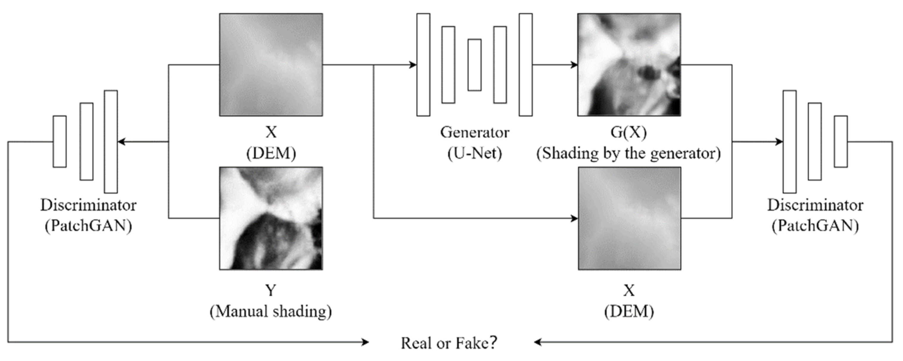
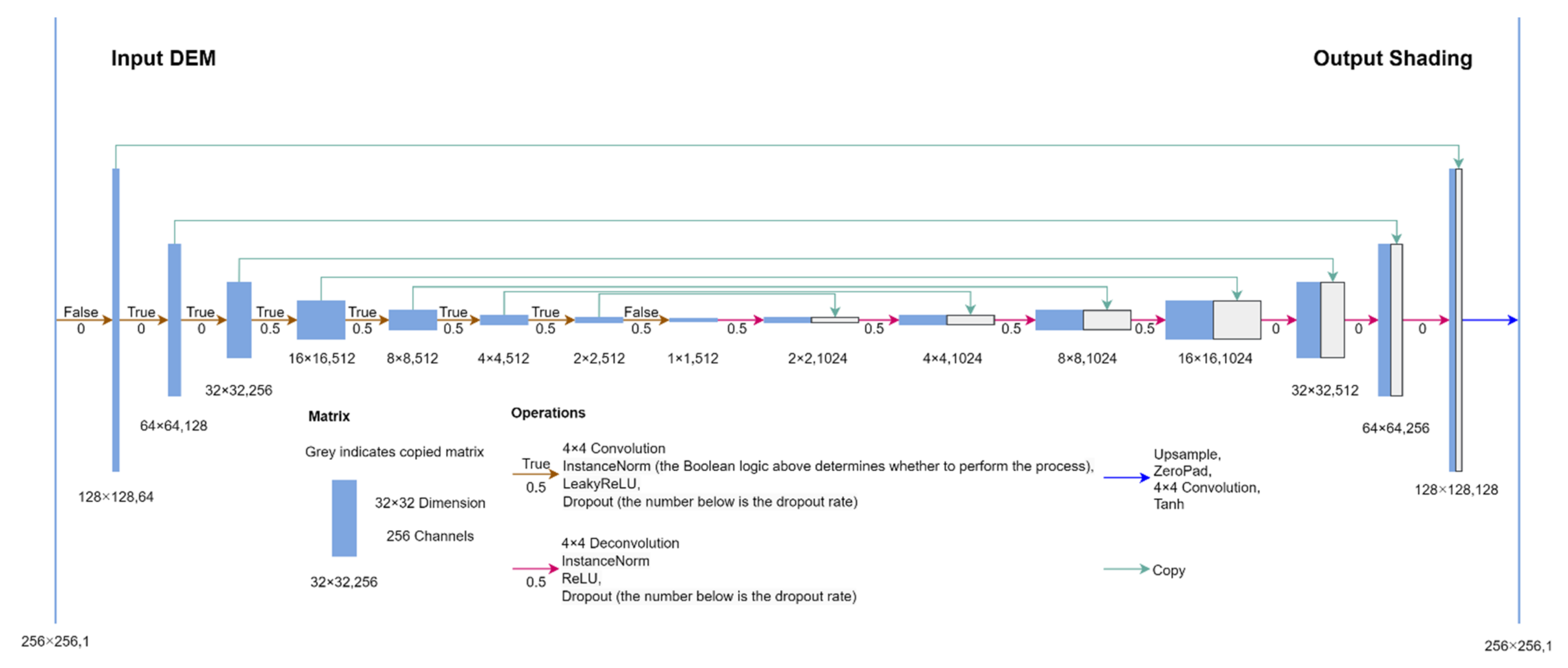
3.1. Network Architecture

GAN and improved GAN have been successfully applied to a range of fields, including image synthesis, style transfer, image super-resolution, and classification. In contrast to deep learning models with only a single network, there are two different networks in GAN: the generator (G) and the discriminator (D). When training the model, the generator learns the hidden features of the sample images so as to improve the authenticity of the generated images to eventually deceive the discriminator, and the discriminator determines if the input image is generated (i.e., fake) or not generated (i.e., real) to the degree possible. The ultimate goal of this competition between the two networks is for the images generated by the generator to sufficiently resemble the real images. Since GAN lacks constraints and its output results are uncontrollable, Mirza et al. [6] introduced an additional constraint in the generator and discriminator of the GAN to obtain a cGAN. The objective function [6] of the cGAN is as follows:

$$cGAN=\underset{G}{\min } \underset{D}{\max } L_{cGAN}(D,G),$$

(1)

$$L_{cGAN}(D,G)=E_{x{~\mathrm{P}}_{data}(x)}\left[\log D(x|y)\right]+E_{z{~\mathrm{P}}_z(z)}\left[\log (1-D(G(z|y)))\right],$$

(2)

where $x$ represents the real value, $y$ represents the condition variable, $z$ represents random noise; $P_{data}(x)$ represents the distribution of real images, $P_{\mathrm{z}}(z)$ represents the a priori noise distribution; $D(x|y)$ represents the probability of real data $x$ being determined as real by $D$ given condition variable $y$; and $G(z|y)$ represents the generated data obtained by inputting noise $z$ and the condition variable $y$ into $G$.

The pix2pix [30] is a special cGAN that generates an output image based on the input image, thus achieving image-to-image translation. Similar to pix2pix, the network proposed in this paper consists of two components: a U-Net generator and a PatchGAN discriminator [30]. The network structure is as shown in Figure 2.

U-Net was first applied for image segmentation in the medical field [29]. Subsequently, it was shown that U-Net can also be effectively applied for the image segmentation of geospatial raster data [31]. U-Net consists of a down-sampling (encoding) process for extracting spatial features and an up-sampling (decoding) process for precise localisation. In the down-sampling process, multi-scale features are obtained by performing multiple convolutions and max pooling processes on the input image. In the up-sampling process, the target image is gradually generated by performing multiple deconvolutions on the extracted features. A skip connection exists between the down-sampling component and the up-sampling component on the same level; this copies the features acquired in the down-sampling process to the corresponding up-sampling process, thus enabling the network to combine low-level and high-level features when generating images. The U-Net structure adopted in this paper is shown in Figure 3, which presents an illustrative scenario with a single channel DEM with a size of 256 × 256 pixels as the input and a single channel network shading of the same size as the output.

The discriminator in GANs usually maps the input sample directly to a real number, which represents the probability that the input sample is a true sample. In contrast, the discriminator in PatchGAN performs multiple convolutions on the input image and maps it to a feature map of size N × N. When judging if the input image is real, PatchGAN first determines if each N × N patch is real, and then takes the average of all patch judgment results as the final judgment result. The feature map is the result of the convolutions, indicating that PatchGAN is in essence a convolutional network. Each pixel of the feature map corresponds to a certain area of the input image (i.e., the receptive field). The size of the receptive field of PatchGAN changes according to the number of convolutions, which can be calculated using the following equation:

$$V_n=(k_n-1){\displaystyle \prod _{i=1}^{n-1}{s}_i}+V_{n-1},n\ge 2,$$

(3)

where $V_n$ represents the receptive field of the $n$-th layer; $V_{n-1}$ represents the receptive field of the ($n-1$)-th layer; $V_0=1,V_1=k_1$; $s_i$ represents the step size of the $i$-th convolution layer; and $k_n$ represents the size of the convolution kernel of the $n$-th layer.

The objective function of this paper combines L1 loss and cGAN loss [30], as follows:

$$G^{*}=\arg \underset{G}{\min } \underset{D}{\max } L_{cGAN}(D,G)+\lambda L_{L1}(G),$$

(4)

$$L_{L1}(G)=E[\left|\right| \mathrm{y}-G(x,y)|{|}_1],$$

(5)

where $\lambda$ represents the coefficient of the penalty term.

3.2. Data and Pre-Processing

The maps produced by Switzerland’s national mapping agency (Swisstopo, Wabern, Switzerland) are precise and beautiful and have long been regarded as the benchmark in the industry. Swisstopo possesses a georeferenced digital manual relief shading product that can easily be used after being aligned with the DEM. In this paper, the 1:500 k scaled manual relief shading produced by Swisstopo and the Shuttle Radar Topography Mission (SRTM) 90 m resolution DEM of the corresponding geographical area were used as the experimental data, as shown in Figure 4. The experimental data cover an area of 316 km × 452 km, including Switzerland and its surrounding areas, with an elevation ranging between 12 m and 4471 m and mainly containing three types of terrain: mountains, hills, and plains.

Since the flat areas in the manual relief shading are generally represented using a grey tone, the bright areas where the lakes are located in the manual relief shading are filled with a continuous grey tone in Adobe Photoshop (Adobe, San Jose, CA, USA) after referring to the distribution of lakes in the experimental area. Moreover, since the coordinate systems of the manual relief shading and the DEM are the CH1903+/LV95 LN02 projection coordinate system and the World Geodetic System 1984 (WGS84) geographic coordinate system, respectively, projection transform is performed on the DEM such that its coordinate system becomes consistent with that of the shading. The shading and the DEM are then resampled to have a cell size of 100 m so as to ensure that each pixel covers an area of the same size. In addition, the shading and the DEM are normalised between 0 and 1. Finally, the manual relief shading and the DEM are segmented while maintaining the corresponding relationship between the two. Each slice contains 256 × 256 pixels, and any slices that are not complete are discarded. Ultimately, a final value of 200 slices each is obtained for manual relief shading and the DEM.

3.3. Network Training and Output

The hardware and environment used for network training were the Ubuntu 18.04 system (with 64 GB memory) and the Quadro A2000 graphics card (with 6 GB of video memory). The network was constructed and trained using Pytorch 1.10, a deep learning open-source library (https://pytorch.org/, accessed on 15 May 2022), and Python 3.9 (Python, Fredericksburg, VA, USA; https://www.python.org/, accessed on 15 May 2022). During network training, the weights were initialised according to the method proposed by He et al. [32], the number of training iterations was set to 500, the learning rate was 0.001, and the Adam optimiser [33] was adopted to optimise the training.

In general, a large number of samples was necessary to train the model to obtain good generalisation ability. When the number of training samples was small, it was possible to expand the sample size through data augmentation (DA), including through mirroring and rotation. Similar operations were carried out in this paper. However, our results indicate that, although such operations successfully increased the number of training samples, the visual effect of the network-shaded relief significantly deteriorated. Due to the scarcity of high-quality georeferenced manual relief shading, the training samples used in this paper comprised 200 pairs of manual relief shading and DEM slices of the corresponding geographical area obtained through pre-processing.

When applying the trained network for rendering a DEM, it is necessary to segment the normalised DEM into slices which are then input into the network. The U-Net generator contains only convolution layers. Training the network is in fact a process of solving for the parameters of the convolution kernel (which are not influenced by the size of the input images). As such, the size of the input DEM slices can be adjusted as needed. Nevertheless, the size needs to be a power of two, such as 256 × 256, 512 × 512, 1024 × 1024, and so on.

In the process of manual relief shading, cartographers adjust the illumination and generalise the terrain while taking into consideration the relationship between the local area and the main terrain so as to enhance the expressiveness of the main terrain. Therefore, each network shading slice only retains its central area as the final generated result. Based on the findings of Jenny et al. [28], the network shading is segmented from a slice of 256 × 256 pixels into a slice of 156 × 156 pixels. The area considered (in addition to the final output area) accounts for 63% of the input slices, which is even greater than the final output area, thus helping the network to fully consider terrain outside the output area to more efficiently generalise the terrain and adjust the illumination.

The network shading generated in blocks needs to be spliced. However, when the edges of adjacent slices differ too greatly in terms of pixel value, the visual effect is severely affected due to obvious splicing marks. Therefore, it is necessary to ensure that the final output slices contain overlapping areas. Hence, alpha blending is used to reduce the pixel value difference between the edges of adjacent slices. Assuming slice A is located at the left or at the top within the adjacent pair, for each row or column the blending is carried by following Equation (6):

$$V_i(O)=\frac{n-i}{n}{V}_i(A)+\frac{i}{n}{V}_i(B),$$

(6)

where $V_i(A), V_i(B)$ represent the respective pixel values of the $i$-th pixel from left to right (or from top to bottom) in the overlapping area between slice A and slice B; $V_i(O)$ represents the pixel value after blending; and $n$ represents the number of pixels in each row or column of the overlapping area.

4. Results and Discussion

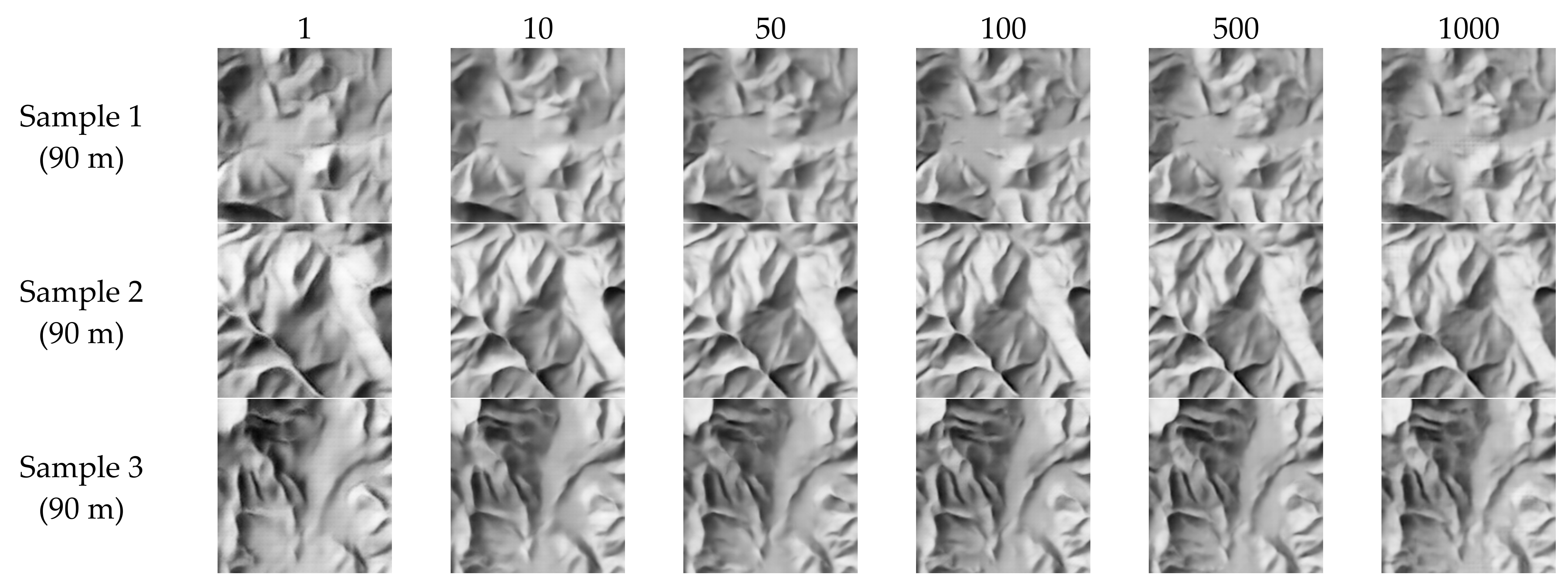
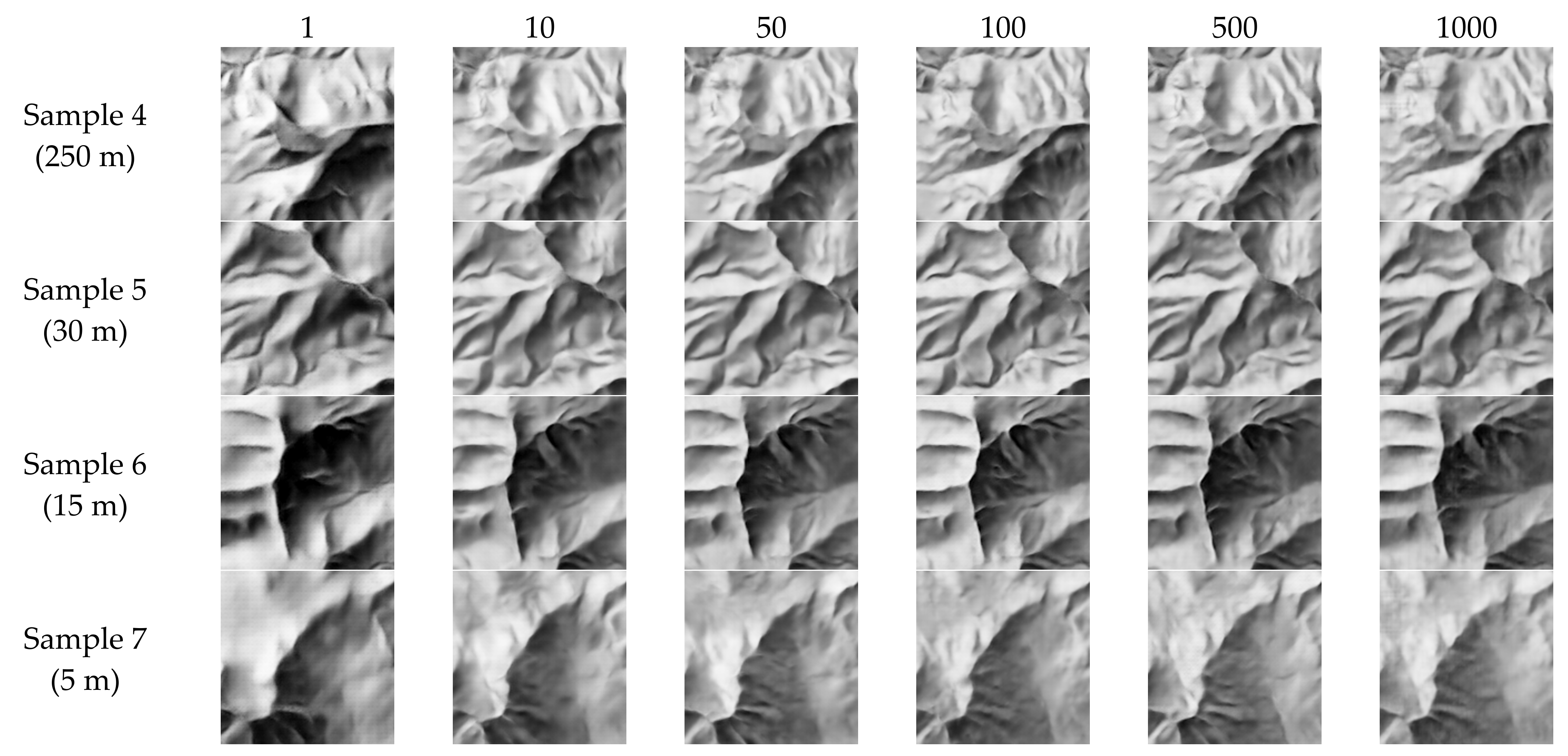
4.1. Determination of Hyperparameters

Deep learning is often regarded as a black-box model, and it is difficult to define the parameters in the network clearly. To ensure that the network can generate high-quality relief shading, enumeration and control variables were used in this paper to explore the settings of the following two hyperparameters: the penalty term coefficient and the size of the PatchGAN receptive field. Due to the lack of standard reference images for comparative calculation and the fact that high-quality shaded relief has intrinsic artistic value, it is very difficult to adopt the loss function or other similar indicators to quantitatively evaluate shaded relief. Instead, visual qualitative inspection was used to evaluate differences in shaded relief.

Networks with different $\lambda$ values were trained with the same dataset, and 90 m resolution DEM slices outside the training set area were also input into the network. Figure 5 shows the shaded relief generated by networks with $\lambda$ values of 1, 10, 50, 100, 500, and 1000, respectively. It can be seen from Figure 5 that obvious mosaics appear in the shaded relief generated by the networks with $\lambda$ values of 1 and 1000, respectively, which affects the overall visual presentation of the relief shading. In addition, as the penalty term coefficient $\lambda$ increases from 1 to 50, more terrain details can be observed in the shaded relief. In contrast, when the penalty term coefficient $\lambda$ increases further from 50 to 1000, the terrain details in the shaded relief do not increase significantly.

To explore the comparative performance of networks with different $\lambda$ values on other scales, the same test was carried out with DEM slices of 5 m, 15 m, 30 m, 250 m, and 500 m resolution, respectively, with results as shown in Figure 6. It can be seen from Figure 6 that mosaics not only appear in the shaded relief generated by the networks with $\lambda$ values of 1 and 1000, but also in the network with a $\lambda$ value of 500 (albeit slightly). Moreover, when the $\lambda$ value is relatively small, although the strong contrast in brightness between the two sides of the ridge enhances the three-dimensionality of the terrain, the overall grey value of the shady slope of the mountain is large and lacks distinction, resulting in a lack of terrain details. In terms of the characterisation of details, when the $\lambda$ value increases from 1 to 50, the terrain details increase in number; yet when the $\lambda$ value increases further from 100 to 1000, the terrain details do not change significantly. This is due to the change in the relative weights of cGAN loss and L1 loss in the objective function, as shown in Equation (4). L1 loss calculates the difference between each pixel of the network shading and the manual shading, whereas cGAN loss measures the difference within a certain region between the two (according to the characteristics of PatchGAN). Since $\lambda$ is the coefficient of the penalty term L1 loss, the objective function becomes more sensitive to the slight difference between the network shading and the manual shading when the value of $\lambda$ increases. To reduce the loss of the objective function, the network enhances the rendering of the detailed terrain features. However, when the value of $\lambda$ exceeds 100, the relative weights of these two losses differ by two orders of magnitude, such that further increasing of the $\lambda$ value fails to bring about an increase in terrain details.

The other hyperparameter studied herein is the size of the PatchGAN receptive field, which is determined by the number of convolution layers. Figure 7 shows the shaded relief generated by the corresponding networks when the PatchGAN receptive field has a size of 7 × 7, 16 × 16, 34 × 34, 70 × 70, or 142 × 142, respectively. It can be seen from Figure 7 that when the size of the PatchGAN receptive field differs, the difference in the relief shading effect is mainly manifested in the terrain characterisation. When the PatchGAN receptive field is of size 7 × 7 and 142 × 142, the network shading of multiple scales shows a slightly blurred characterisation of the sharp ridges. When the PatchGAN receptive field is of size 142 × 142, the network shading appears to be granular when the cell size is large (90 m, 250 m). When the PatchGAN receptive field is of size 16 × 16, 34 × 34, and 70 × 70, the network shading is not much different in terms of overall visual effect.

To achieve the desired relief shading effect, it is necessary to redefine $\lambda$ and the receptive field size when other datasets are applied. Taking into consideration the degree of generalisation of the terrain, the contrast between bright and shaded sides, and the overall visual effect, the penalty term coefficient $\lambda$ was taken as 100, and the size of the PatchGAN receptive field was set to 70 × 70 for the sample dataset used in this paper.

4.2. Comparison with Analytical Shading

To compare the network shading with the analytical shading generated by different software packages, a DEM outside Switzerland was selected for shaded relief generation. We used a laptop on which 2020 Windows OS (Microsoft, Seattle, WA, USA) was installed (GPU, model NVIDIA GeForce RTX 2060). The mountainous area of western Tibet was selected (${76.623}^{\circ }~{78.575}^{\circ }$ E, ${33.606}^{\circ }~{34.936}^{\circ }$ N), with an elevation ranging from 2634 m to 7598 m. The DEM slices had a resolution of 90 m and contained a total of 1780 × 1432 pixels. The selected area has multiple mountains that strike in different directions. Figure 8 shows the DEM and three types of shaded relief in this area. The network shading (with an input DEM slice of 256 × 256 pixels and output shaded relief of 156 × 156 pixels, and where adjacent slices have an overlapping area of 40 pixels) took 8 s for rendering. QGIS was adopted for diffuse shading (with a vertical angle of ${45}^{°}$, an azimuth of ${315}^{°}$, and a z factor of 1); this took 0.4 s for rendering. Skylum [34] was adopted for clear sky shading (with a z factor of ${45}^{°}$ and an azimuth of ${315}^{°}$); this took 598 s for rendering. Since the three types of shaded relief differ in terms of brightness and contrast, these were adjusted to approximately the same values to compare the expressiveness of the shaded relief.

It can be seen from Figure 8 that the network shading (b) differs significantly from the two analytical shading depictions (c,d), as the network successfully simulated the artistic style of manual relief shading by Swiss cartographers, producing Swiss-style shaded relief. In addition, the ability to accurately represent the terrain as well as the relationship between terrain elements is the most basic requirement for relief shading. A comparison reveals that the spatial distribution of mountains and valleys in the network shading is in good agreement with that of the two analytical relief shadings, ensuring the accuracy of the terrain position. Moreover, the network shading showed no non-existent terrain elements and likewise did not miss any major terrain elements.

On top of meeting the basic requirement for relief shading, the network shading successfully generalised the terrain. This can easily be observed by comparing the different types of shaded relief; the network shading led to fewer broken terrain details while emphasising the main terrain structures, hence allowing the readers to grasp the terrain characteristics of the area more easily and quickly. Shaded relief is usually not applied alone; instead, additional geographical features such as rivers, roads, and residential areas are often superimposed onto the shaded relief. As such, if a large number of broken terrain details exist in the shaded relief, the map is made unnecessarily complicated; this is unconducive to the expression of other features. The network shading shown herein depicts complete mountains clearly drawn, making this end product suitable to be used as the base map for more complicated terrains.

In addition, the network shading successfully simulated the local illumination adjustment evident in the manual shading. Region A in Figure 8a shows a northwest-trending mountain range at the bottom left of the mapping area. Since this mountain range is in the same direction as the main illumination, it can hardly be recognised in diffuse shading and clear sky shading. In contrast, network shading is capable of adjusting the illumination direction locally and is thus capable of rendering this mountain range clearly visible. In an even smaller area, such as regions B, C, and D in Figure 8a, the network shading adjusted the contrast between the two sides of the ridge through illumination adjustment, further enhancing the expressiveness of the shading. For example, in regions E and F in Figure 8a, clear sky shading deepened the tone of narrow valleys and increased the brightness of ridges in comparison with diffuse shading, which improved the three-dimensionality to a certain extent. Nevertheless, the expressiveness of terrains was still much poorer than that of network shading.

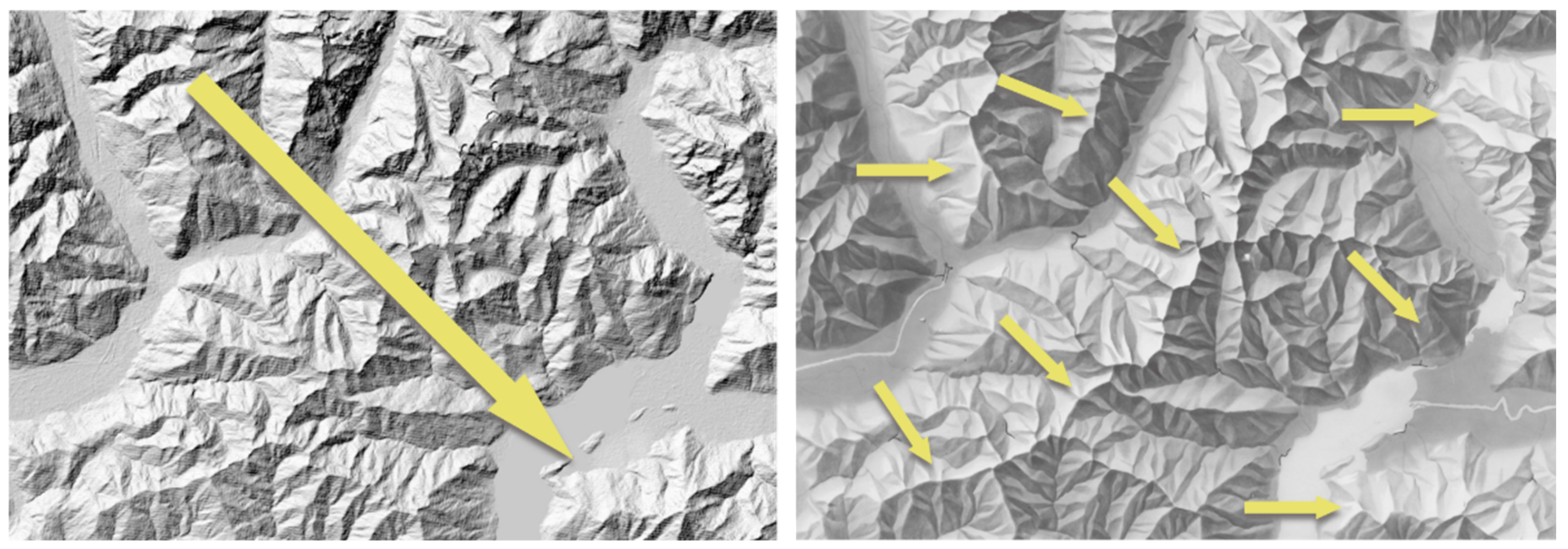
4.3. Comparison with Manual Shading

Manual relief shading outside Switzerland was selected from the Shaded Relief Archive [35], and the DEM of corresponding areas was input into the network to generate relief shading. The comparison between network shading and manual shading is shown in Figure 9. Due to the overall dark tone and strong contrast of the manual relief shading used for training, the network shading also shows similar characteristics. As such, the brightness and contrast of the network shading were adjusted in QGIS such that the network shading became similar in tone to the corresponding manual relief shading. Due to the lack of data information and projection information used for the manual relief shading, differences exist locally between the network shading (via the DEM) and the corresponding manual shading.

The comparison between manual shading and network shading indicates that the two end products differ in various aspects. In terms of terrain generalisation, the network shading has a low degree of generalisation when describing areas with gentle elevation changes due to the lack of these areas in the dataset used for training. When depicting mountainous areas with large elevation changes, the degree of generalisation of network shading and manual shading was roughly the same. In addition, the network seems to use the same generalisation scale for the entire shaded relief, whereas manual shading adjusts the generalisation scale locally according to regional features to fully reflect the terrain features. As shown by the two pairs of shaded relief provided in Figure 9 (i.e., (a–d)), when the degree of generalisation of the mountainous areas is generally the same, manual shading shows a higher degree of generalisation in terrains with gentle changes as compared with network shading.

In terms of terrain characterisation, the network shading was not as detailed as the manual shading. The areas at relatively low altitudes with gentle terrain changes showed smaller changes in tone in the network shading. In contrast, the corresponding areas in the manual shading showed more detailed tone changes and details, making the visual effect more artistic. This is shown in the right region in Figure 9b, the central and left regions in Figure 9d, the central and upper regions in Figure 9f, and the valleys in Figure 9g. It can be seen from these regions that the cartographers adjust their drawing methods or adopt exaggeration according to not only the terrain features but also to other geographical elements (such as rivers and lakes), as well as to the relationship between terrain features. In contrast, network shading is rendered based only on DEM slices by a network trained with relief shading and DEM. As a result, the northwest-trending mountain range in the centre of Figure 9c is hardly recognisable, but is rather easily recognised as shown in Figure 9d; this is due to the emphasis placed on this part of the terrain during manual shading.

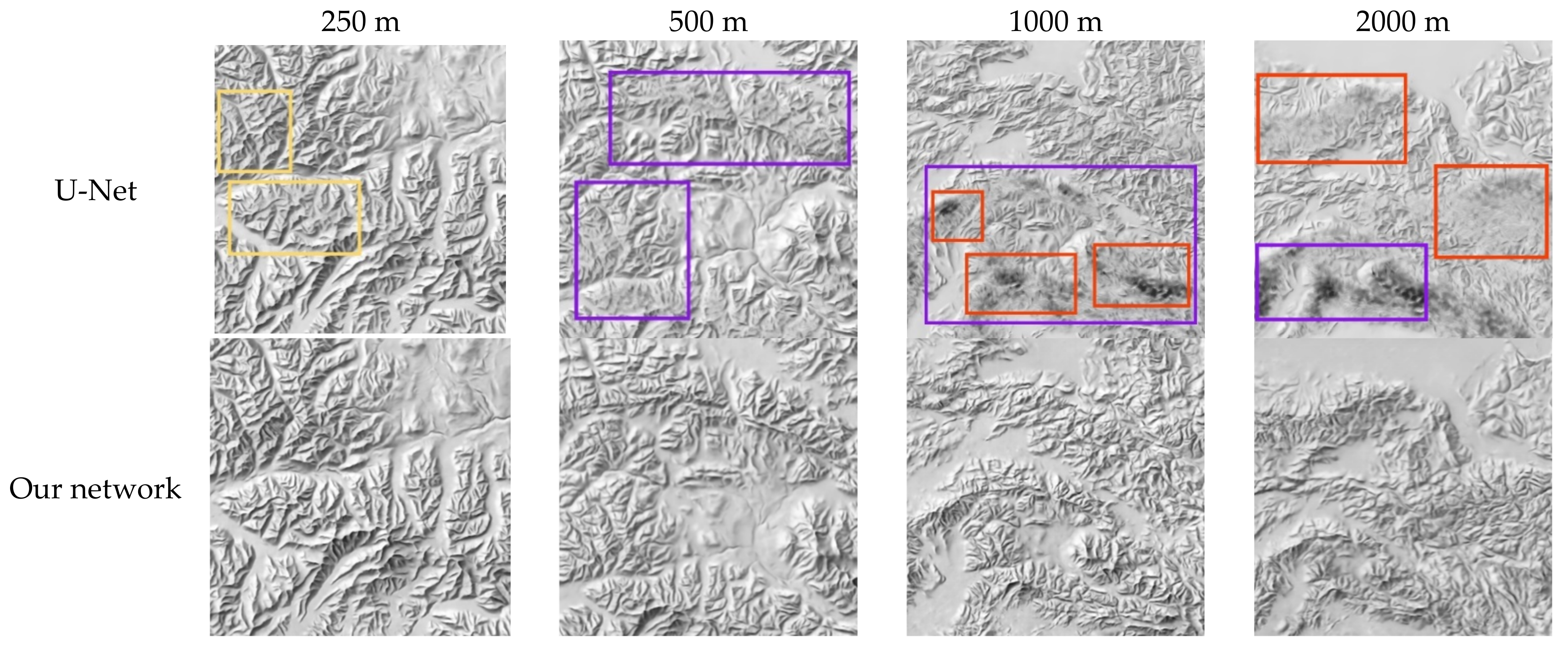
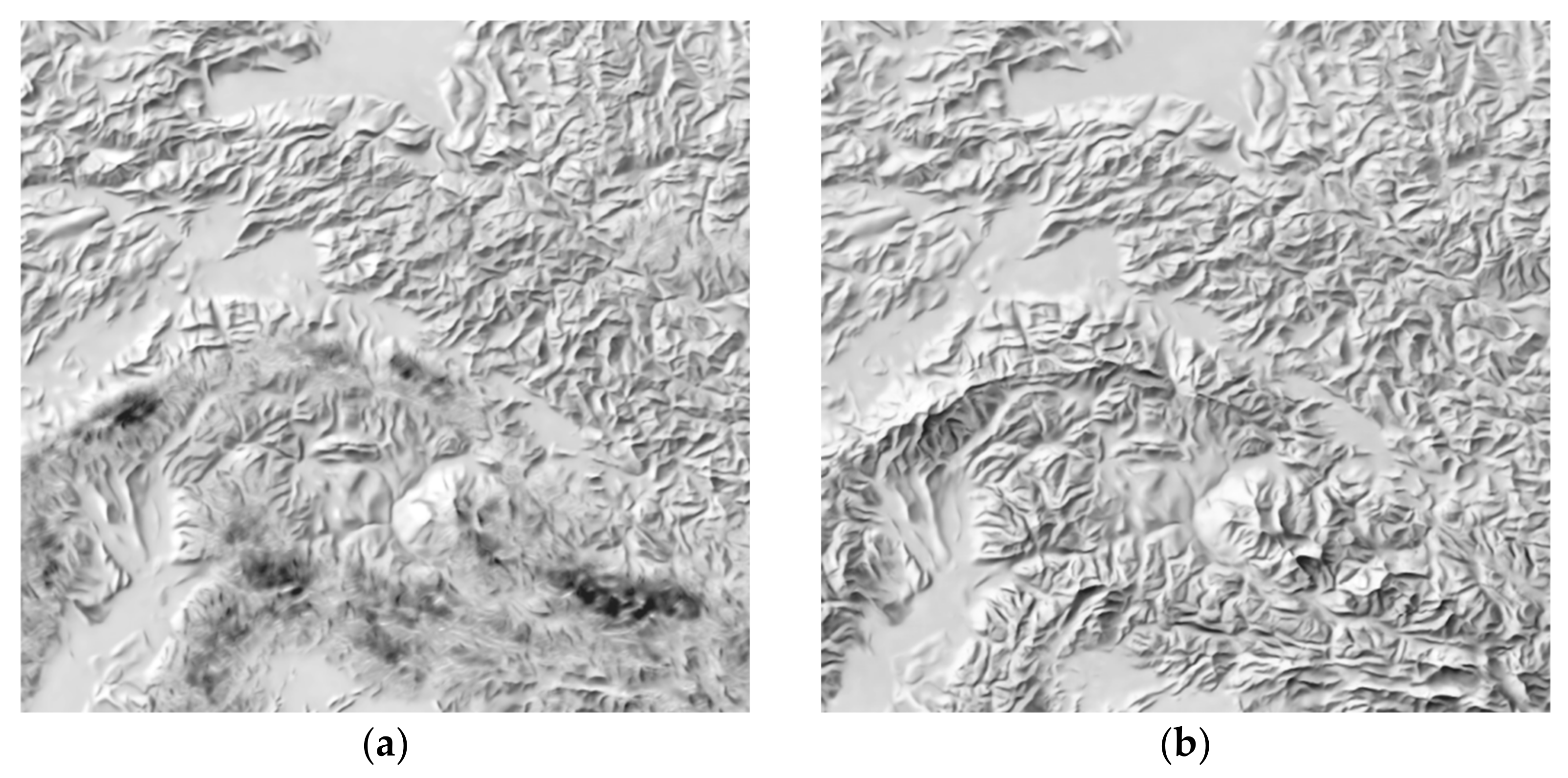
4.4. Comparison with Other Methods

In this paper, a previously U-Net network [28] was trained with the same training data set for 2000 epochs. Both the prior U-Net [28] and the adapted network proposed in this paper were used for shading with a multi-scale DEM [36]. Figure 10 and Figure 11 show the shaded relief generated using the different networks and with a DEM of different cell sizes. As shown in Figure 10, the contrast between the two sides of the mountain ridges in the shaded relief generated by the proposed method is stronger and the sharp ridges are shown more clearly; this becomes more obvious when the cell sizes of the DEM become smaller. In general, when the cell size of the DEM is smaller than that of the training data, the network proposed in this paper performs better.

The difference between the two networks became more significant when the DEM cell size was larger than that of the training data. As shown in Figure 11, when handling a 250 m resolution DEM, the U-Net network [28] failed to render the mountainous areas in the centre and upper left corner well, as the tones on the two sides of the ridge are almost the same (as shown by the yellow box in Figure 11). As the cell size increased, this failed shading became more and more obvious (as shown by the purple box in Figure 11), such that large areas of black regions appear (as shown by the red box in Figure 11), thereby severely undercutting the identification of terrain features and visual effects. The network proposed in this paper was able to avoid such situations by generating shaded relief of a cell size that was rather different from that of the training data with a good visual effect. Nevertheless, when the DEM cell size is 2000 m, the sharpness of terrain features in the shaded relief is lost to a large extent. It is thus suggested that the DEM cell size should not exceed 10 times that of the training data.

We also trained the U-Net network in this paper alone (i.e., without the discriminator) and trained the referenced U-Net network [28] as a generator in pix2pix (with a discriminator). The trained networks are used for rendering DEMs with cell sizes of 1000 m, as shown in Figure 12. It can be observed that, without the adversarial structure, shaded relief achieved by the U-Net network adapted in this paper shows large areas of black regions. In contrast, the proposed U-Net [28] with an adversarial structure was successful in rendering the otherwise black regions (shown in Figure 11). This indicates that the adversarial structure can help enhance the shading effect when the cell size is relatively large (in comparison with that of the training data). However, the proposed U-Net network [28] with an adversarial structure failed to improve the blurred features when cell sizes were relatively small.

5. Conclusions

To improve the quality of shaded relief, this paper introduced a cGAN from within the field of deep learning, taking manual shaded relief and the corresponding DEM as the dataset to propose a shaded relief generation method based on the cGAN. The lakes in the manual shaded relief were first coloured, while projection was carried out for the DEM slices, followed by resampling, normalisation, and segmentation to form the manual shaded relief-DEM slice as the training dataset. Subsequently, the established cGAN was trained under supervision. Finally, the DEM of any area was input into the network, and the output results of which were processed with alpha blending and spliced to form the network shading.

Our test results indicate that the network successfully simulated the manual shading style of Swiss cartographers, greatly enhancing the artistic effect of the shaded relief. The trained network emphasised the main terrain features while reducing the broken terrain details, achieving terrain generalisation relatively well. At the same time, the network was capable of simulating illumination adjustments completed according to local terrain features in manual shading, hence enhancing the expressiveness of the terrain. Although the network shading still cannot match the visual effect of manual shading, it nevertheless shows great improvement when compared with analytical shading. Moreover, compared with existing networks, the method proposed in this paper solves the problem of blurring in a portion of the terrain features, with clearer feature characterisation. In addition, the proposed method shows better and more stable performance when the shaded relief and training data have very different cell sizes, which can be attributed to the adversarial structure of this network.

The proposed method nevertheless has certain limitations. Firstly, for shading given a DEM with a large flat area and with only gentle changes, noise appears in the flat area of the generated shaded relief. Secondly, it is not as flexible as manual shading in terms of terrain generalisation, such that only one generalisation scale can be adopted by the entire mapping area and it is impossible to adjust the generalisation scale according to the local terrain (as in manual shading). Thirdly, given a DEM with a cell size that is greater than that of the training data (for example, a DEM with a cell size that is 20 times larger than the training dataset), the generated shaded relief has a good visual effect overall, but the clarity of the mountains is lost to a large extent. In future work, we plan to increase the sample data and to test this methodology with more networks and modules to solve the existing problems and further improve the shading effect. This study can allow cartographers to obtain high-quality shaded relief more easily to produce even more beautiful maps.

References

1. Wang, J.; Sun, Q.; Wang, G.; Jiang, N.; Lyu, X. Principle and Method of Cartography, 2nd ed.; Science Press: Beijing, China, 2014. [Google Scholar]
2. Girshick, R.; Donahue, J.; Darrell, T.; Malik, J. Rich Feature Hierarchies for Accurate Object Detection and Semantic Segmentation. In Proceedings of the 2014 IEEE Conference on Computer Vision and Pattern Recognition, Columbus, OH, USA, 23–28 June 2014; IEEE Publications: Columbus, OH, USA, 2014; pp. 580–587. [Google Scholar] [CrossRef] [Green Version]
3. Krizhevsky, A.; Sutskever, I.; Hinton, G.E. ImageNet Classification with Deep Convolutional Neural Networks. Commun. ACM 2017, 60, 84–90. [Google Scholar] [CrossRef]
4. Long, J.; Shelhamer, E.; Darrell, T. Fully Convolutional Networks for Semantic Segmentation. In Proceedings of the 2015 IEEE Conference on Computer Vision and Pattern Recognition (CVPR), Boston, MA, USA, 7–12 June 2015; IEEE Publications: Boston, MA, USA, 2015; pp. 3431–3440. [Google Scholar] [CrossRef] [Green Version]
5. Goodfellow, I.; Pouget-Abadie, J.; Mirza, M.; Xu, B.; Warde-Farley, D.; Ozair, S.; Courville, A.; Bengio, Y. Generative Adversarial Networks. Commun. ACM 2020, 63, 139–144. [Google Scholar] [CrossRef]
6. Mirza, M.; Osindero, S. Conditional Generative Adversarial Nets. arXiv 2014, arXiv:1411.1784. [Google Scholar]
7. Creswell, A.; White, T.; Dumoulin, V.; Arulkumaran, K.; SenGupta, B.; Bharath, A.A. Generative Adversarial Networks: An Overview. IEEE Signal Process. Mag. 2018, 35, 53–65. [Google Scholar] [CrossRef] [Green Version]
8. Dong, Y.; Tang, G. Research on Terrain Simplification Using Terrain Significance Information Index From Digital Elevation Models. Geomat. Inf. Sci. Wuhan Univ. 2013, 38, 353–357. [Google Scholar] [CrossRef]
9. Ai, T.; Li, J. A DEM Generalization by Minor Valley Branch Detection and Grid Filling. ISPRS J. Photogramm. Remote Sens. 2010, 65, 198–207. [Google Scholar] [CrossRef]
10. Li, J.; Li, D. A DEM Generalization by Catchment Area Combination. Geomat. Inf. Sci. Wuhan Univ. 2015, 40, 1095–1099. [Google Scholar] [CrossRef]
11. Geisthövel, R.; Hurni, L. Automated Swiss-Style Relief Shading and Rock Hachuring. Cartogr. J. 2018, 55, 341–361. [Google Scholar] [CrossRef]
12. Jenny, B. Terrain Generalization With Line Integral Convolution. Cartogr. Geogr. Inf. Sci. 2021, 48, 78–92. [Google Scholar] [CrossRef]
13. He, Z.; Guo, Q.; Zhao, M.; Liu, J.; Zhang, J.; Li, X.; Liang, Z. Research on DEM Automatic Generalisation in Complex Geomorphic Areas Based on Wavelet Analysis. Geogr. Geo-Inf. Sci. 2019, 4, 57–63. [Google Scholar]
14. Lindsay, J.B.; Francioni, A.; Cockburn, J.M.H. LiDAR DEM Smoothing and the Preservation of Drainage Features. Remote Sens. 2019, 11, 1926. [Google Scholar] [CrossRef] [Green Version]
15. Raposo, P. Variable DEM Generalization Using Local Entropy for Terrain Representation Through Scale. Int. J. Cartogr. 2020, 6, 99–120. [Google Scholar] [CrossRef]
16. Yu, W.; Zhang, Y.; Ai, T.; Chen, Z. An Integrated Method for DEM Simplification With Terrain Structural Features and Smooth Morphology Preserved. Int. J. Geogr. Inf. Sci. 2021, 35, 273–295. [Google Scholar] [CrossRef]
17. Imhof, E. Cartographic Relief Presentation; ESRI Press: Redlands, CA, USA, 2007. [Google Scholar]
18. Jenny, B. An Interactive Approach to Analytical Relief Shading. Cartographica 2001, 38, 67–75. [Google Scholar] [CrossRef]
19. Marston, B.E.; Jenny, B. Improving the Representation of Major Landforms in Analytical Relief Shading. Int. J. Geogr. Inf. Sci. 2015, 29, 1144–1165. [Google Scholar] [CrossRef]
20. Veronesi, F.; Hurni, L. A GIS Tool to Increase the Visual Quality of Relief Shading by Automatically Changing the Light Direction. Comput. Geosci. 2015, 74, 121–127. [Google Scholar] [CrossRef]
21. Veronesi, F.; Hurni, L. Changing the Light Azimuth in Shaded Relief Representation by Clustering Aspect. Cartogr. J. 2014, 51, 291–300. [Google Scholar] [CrossRef]
22. Kennelly, P.J.; Stewart, A.J. General Sky Models for Illuminating Terrains. Int. J. Geogr. Inf. Sci. 2014, 28, 383–406. [Google Scholar] [CrossRef]
23. Florinsky, I.V.; Filippov, S.V. Three-Dimensional Terrain Modeling with Multiple-Source Illumination. Trans. GIS 2019, 23, 937–959. [Google Scholar] [CrossRef]
24. Kennelly, P.J. Terrain Maps Displaying Hill-Shading with Curvature. Geomorphology 2008, 102, 567–577. [Google Scholar] [CrossRef]
25. Podobnikar, T. Multidirectional Visibility Index for Analytical Shading Enhancement. Cartogr. J. 2012, 49, 195–207. [Google Scholar] [CrossRef]
26. LeCun, Y.; Bengio, Y.; Hinton, G. Deep Learning. Nature 2015, 521, 436–444. [Google Scholar] [CrossRef]
27. Patterson, T. Designing the Equal Earth Physical Map. Available online: https://youtu.be/UYQ6vhxc9Dw (accessed on 8 April 2022).
28. Jenny, B.; Heitzler, M.; Singh, D.; Farmakis-Serebryakova, M.; Liu, J.C.; Hurni, L. Cartographic Relief Shading with Neural Networks. IEEE Trans. Vis. Comput. Graph. 2021, 27, 1225–1235. [Google Scholar] [CrossRef]
29. Ronneberger, O.; Fischer, P.; Brox, T. U-Net: Convolutional Networks for Biomedical Image Segmentation. In Medical Image Computing and Computer-Assisted Intervention 2015; Navab, N., Hornegger, J., Wells, W.M., Frangi, A.F., Eds.; Springer International Publishing: Cham, Switzerland, 2015; Volume 9351, pp. 234–241. [Google Scholar] [CrossRef] [Green Version]
30. Isola, P.; Zhu, J.-Y.; Zhou, T.; Efros, A.A. Image-to-Image Translation with Conditional Adversarial Networks. In Proceedings of the 2017 IEEE Conference on Computer Vision and Pattern Recognition (CVPR), Honolulu, HI, USA, 21–26 July 2017; IEEE Publications: Honolulu, HI, USA, 2017; pp. 5967–5976. [Google Scholar] [CrossRef] [Green Version]
31. Heitzler, M.; Hurni, L. Cartographic Reconstruction of Building Footprints from Historical Maps: A Study on the Swiss Siegfried Map. Trans. GIS 2020, 24, 442–461.32. [Google Scholar] [CrossRef]
32. He, K.; Zhang, X.; Ren, S.; Sun, J. Delving Deep into Rectifiers: Surpassing Human-Level Performance on ImageNet Classification. In Proceedings of the 2015 IEEE International Conference on Computer Vision (ICCV), Santiago, Chile, 7–13 December 2015; IEEE Publications: Santiago, Chile, 2015; pp. 1026–1034. [Google Scholar] [CrossRef] [Green Version]
33. Kingma, D.P.; Ba, J. Adam: A Method for Stochastic Optimization. arXiv 2017, arXiv:1412.6980. [Google Scholar]
34. Sky Models. Available online: http://watkins.cs.queensu.ca/~jstewart/skyModels.zip (accessed on 8 April 2022).
35. Shaded Relief Archive. Available online: http://www.shadedreliefarchive.com (accessed on 8 April 2022).
36. Kennelly, P.J.; Patterson, T.; Jenny, B.; Huffman, D.P.; Marston, B.E.; Bell, S.; Tait, A.M. Elevation Models for Reproducible Evaluation of Terrain Representation. Cartogr. Geogr. Inf. Sci. 2021, 48, 63–77. [Google Scholar] [CrossRef]
Figure 1. Analytical shading with one direction of illumination (left) and manual shading with illumination adjustments according to local landforms (right). The manually adjusted illumination shows landforms more clearly.
Ijgi 11 00374 g001
Figure 2. Network structure.
Ijgi 11 00374 g002
Figure 3. U-Net structure.
Ijgi 11 00374 g003
Figure 4. Experimental data. (a) manual relief shading (©Swisstopo); and (b) a 90 m resolution DEM of the corresponding area.
Ijgi 11 00374 g004
Figure 5. Shaded relief generated by networks with different values with a 90 m resolution DEM.
Ijgi 11 00374 g005
Figure 6. Shaded relief generated by networks with different values with multi-scale DEM slices.
Ijgi 11 00374 g006
Figure 7. Shaded relief generated by networks with different PatchGAN receptive field sizes in multi-scale DEM slices.
Ijgi 11 00374 g007aIjgi 11 00374 g007b
Figure 8. (a) DEM of the mapping area; (b) network shading; (c) diffuse shading; and (d) clear sky shading.
Ijgi 11 00374 g008aIjgi 11 00374 g008b
Figure 9. Four pairs of network shading (left) and manual shading (right) depictions. The first pair, (a,b), shows terrain in Washington State, USA; the second pair, (c,d), shows terrain in Yellowstone National Park, Wyoming, USA; the third pair, (e,f), shows terrain in the Sinai Peninsula, Egypt; the fourth pair, (g,h), shows terrain in Rocky Mountain National Park, Colorado, USA. Among these images, (a,c,e) were generated using a 90 m resolution DEM, and (g) was generated with a 45 m resolution DEM. The following adjustments were made in QGIS: (a) brightness was adjusted to 20 and contrast was adjusted to −20; (c) brightness was adjusted to 50 and contrast was adjusted to −25; (e) brightness was adjusted to 20 and contrast was adjusted to −20; and (g) brightness was adjusted to 25 and contrast was adjusted to −20.
Ijgi 11 00374 g009aIjgi 11 00374 g009b
Figure 10. Shaded relief generated by different networks and DEMs with a cell size smaller than that of the training data.
Ijgi 11 00374 g010
Figure 11. Shaded relief generated using different networks and DEM with cell sizes greater than that of the training data.
Ijgi 11 00374 g011
Figure 12. Effect of an adversarial structure on shading when the cell size was larger than that in the training data: (a) shaded relief generated by our U-Net without an adversarial structure, and (b) shaded relief generated by the proposed U-Net [28] with an adversarial structure.
Ijgi 11 00374 g012
Publisher’s Note: MDPI stays neutral with regard to jurisdictional claims in published maps and institutional affiliations.