Abstract
Offender residences have become a research focus in the crime literature. However, little attention has been paid to the interactive associations between built environment factors and the residential choices of offenders. Over the past three decades, there has been an unprecedented wave of migrant workers pouring into urban centers for employment in China. Most of them flowed into urban villages within megacities. Weak personnel stability and great mobility have led to the urban villages to be closely related to decreased public safety and the deterioration of social order. The YB district in China was selected as the study area, which is located in one of the most developed cities in Southern China and has an area of approximately 800 km2 and a population of approximately four million people. This study aims to explore the associations between the neighborhood environment and the offender residences by using the geographical detector model (GeoDetector) from the perspective of interaction. The conceptual framework is based on the social disorganization theory. The results found that urban villages were the most important variable with a relatively high explanatory power. In general, taking the urban village as the carrier, various places (hotels, entertainment places, and factories) within the urban village may be more likely to include offender residences. This study also found the social disorganization theory applicable in the non-Western context. These findings may have important implications for offender residences identification, crime prevention, and the management of urban villages in Chinese cities.
1. Introduction
Research on the residential locations of offenders is an important topic in criminology, geography, sociology, and urban disciplines [1]. The pioneering work proposed by Shaw and McKay [2] focused on the spatial distribution of juvenile delinquents in Chicago and found that the rate of young offenders declined from the city center toward the periphery. More recently, the subject has developed in different national contexts. The work of Law et al. indicated that young offenders were mainly concentrated in urban areas in Canada [3], while the work of Liu et al. revealed that juvenile migrant burglars tended to live in communities with high residential instability in China [1]. Furthermore, the studies of different types of crime such as sex crimes [4,5,6] and theft [7] have also shown that offender residences have the characteristics of spatial agglomeration.
The association between offender residences and the urban built environment has become a research focus and has been widely discerned under the guidance of the social disorganization theory. It assumes that the communities with disorganization (i.e., high residential mobility, low socioeconomic status, and high ethnic heterogeneity) have low social cohesion, which leads to a loss of informal social control and an increase in crime levels [8]. Thus, this theory is often selected as the theoretical foundation in the explanation of the association between offender residence and the neighborhood characteristics. Additionally, several empirical studies have shown that the offender rate is strongly associated with social disorganization. Law et al. found that juvenile offending is positively correlated with predictors of social disorganization, such as single-parent families, immigrants, ethnic heterogeneity, and residential mobility [9]. In the study of Breetzke et al., economic deprivation played an important role in the distribution of the offender rate [10]. High offender rates occurred in areas with a high level of economic deprivation, while the affluent areas exhibited low offender rates. Many studies have highlighted the complex interplay between crime and demographic features such as sex, age, income, race and ethnicity, marriage, family structure, etc. [11,12,13,14].
In addition, other theories, such as the routine activity theory, environmental criminology, and the crime pattern theory, have also been applied to the study of offender residences. The routine activity theory acknowledges that the occurrence of most crimes results from the convergence of the presence of likely offenders and suitable targets, and the absence of capable guardians in space and time [15]. The crime pattern theory focuses on the factors that structure criminal opportunities and the major characteristics of the lived environment [16,17,18]. Brantingham and Brantingham hold that potential offenders tend to commit crime near places they know from their everyday activities, such as where they live, work, or socialize; that is, their ‘activity nodes’ [17]. These theories provide an explanation as to why criminal events are concentrated in particular places and times. For example, Bernasco found that offenders who committed robbery, residential burglary, vehicular thefts, and assaults were more likely to target their current and former residential areas than similar areas they had never lived in [19]. Since sex offenders are prone to live in the proximity of potential victims, researchers have analyzed the residences of both offenders and victims simultaneously [20,21]. Additionally, when considering the potential criminal space, some studies have linked the risk of crimes to land use indicators and facilities such as stations, bars, residences, parks, etc. These studies have demonstrated that the proportions of industrial and commercial land use are positively correlated with male offender residence [22], while the proportion of open land use is positively related to young offender residence [3]. Roncek and Bell found there were more crimes on blocks with bars compared with those without bars [23]. Additionally, McCord and Ratcliffe have shown that street robberies tended to occur near subway stations [24]. Concerning outdoor rape, crimes occurred disproportionately near bus stops and bars, but away from the nearest residence [25]. Furthermore, the importance of particular combinations of crime generators and attractors in the proximate environment around public bus stops has been discussed by Hart and Miethe. Compared to other activity nodes, bus stops are more likely to be located across dominant situational profiles of robbery [26]. Researchers have also identified subtle variations in victimization risk across environments based on features of the landscape using risk terrain modeling, which has been used to study different types of crime such as property crime and violent crime [27,28,29,30].
Furthermore, research related to crime and offender residence studies mainly include two aspects: the spatial characteristic of locations and potential factors analysis. In terms of the spatial characteristics of locations, the descriptive analysis of spatial distribution characteristics, hot spot analysis, and kernel density estimation have been the most widely used methods [31,32,33,34,35], as it is pivotal to allocate police resources effectively for crime reduction and prevention [36,37,38,39]. For example, the work of Brownstein et al. identified potential hot spot areas where opioid medication abuse occurred by applying risk mapping and spatial detection methods to identify crime clusters [40]. As a traditional hotspots analysis method, K-means clustering was utilized on a dataset from New South Wales to measure the rates of crimes, including theft, homicide, and various drug offenses in cities with high crime rates [41]. Recently, kernel density estimation (KDE) has been in high demand in crime analysis, since it represents the spatial distribution in a visually appealing and accurate way [42,43,44,45,46]. To analyze the influence of the parameters (i.e., cell size and bandwidth) in the KDE model, comparative experiments have been conducted with different crime data. They found that cell size had little influence, while bandwidth size did have an influence on KDE crime hotspot maps [47,48]. In terms of potential factor analyses, multivariate analysis methods such as Poisson, negative binomial regression, and cross-classified multilevel regression methods have been adopted in several studies [49,50,51]. For example, a negative binomial regression model was used to analyze the factors of offender residence locations in China, and found that a socially disorganized neighborhood with high residential instability was likely to attract more burglars [1]. In general, offender residence locations data are a type of spatial data with geographical location information, so the spatial heterogeneity, which refers to the uneven distribution of variables within a given area, is important [52]. However, spatial heterogeneity is usually ignored in a regression analysis [53,54,55]. This problem can be addressed using the geographical detector (GeoDetector) model. The GeoDetector model proposed by Wang et al. presents a solution for exploring variable spatial associations between phenomena and geographical factors and the impacts of the interactions between these factors [56]. In contrast to multiple regression analysis methods, this model is not affected by collinearity among multiple discretized independent variables [57].
Motivated by the above literature, this work is a case study on offender residences in the YB district, ZG city, based on the social disorganization theory. The theory was chosen for the following reasons: (1) The first research to use this this theory particularly focused on the geographical distribution of offender residences [58]. (2) It emphasizes the significant influence of the social and economic characteristics of local neighborhoods [59], which can help us to interpret the association between offender residences and the community structure. Moreover, existing studies have focused on the associations between offender residences and the neighborhood environment by analyzing the individual association between each factor and offender residences using several types of regression models. However, little attention has been paid to the interactive associations between factors on the offender residence locations. In this study, we used the interaction detector model of GeoDetector to fill this gap. Specifically, we utilized the descriptive analysis and KDE to understand the spatial patterns of offender residences and leveraged the GeoDetector model to reveal the association between the ambient environment factors and the residential locations of offenders. It is expected that the results of this study can provide a reference that would help concerned departments understand the geographical demand for their services and formulate targeted prevention and control policies to reduce the negative impacts of crimes. The overall workflow of the study can be seen in Figure 1.
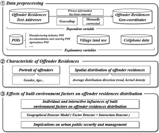
Figure 1.
The workflow of this study.
The remainder of the paper is organized as follows: The relevant materials, including the study area and data, are introduced in Section 2. In Section 3, methods, and research questions are presented. The results and discussions are presented in Section 4. Finally, we provide some concluding remarks in Section 5.
2. Study Area and Data
2.1. Study Area
The real name of the study area cannot be mentioned due to a confidentiality agreement, but it was briefly described here. The YB district is located in one of the most developed cities in Southern China and has an area of approximately 800 km2 and a population of approximately four million people. The study area is the district with the greatest number of urban villages and the largest migrant population in the city (Figure 2). It is dominated by urban villages that attract plenty of migrants to live due to its specialization in the manufacturing of cloth, clothing, leather, and daily cosmetics. The seventh national population census in 2020 stated that there were over 2.3 million nonlocal residents living in the study area. Migrants are categorized into two groups in China’s Household Registration (hukou) system: local and nonlocal residents. That stated, those nonlocal residents are not eligible for social welfare rights such as national medical insurance, welfare housing, etc., to which a local resident (with hukou) is entitles. Nonlocal residents are usually perceived as outsiders in the city. Figure 2 shows the spatial distribution of offender residences and urban villages. In the study area, there are two types of residential land: urban villages and urban residential land. On the one hand, urban villages were symbolized by different-sized circles according to their area (Figure 2), because the real outlines and land use patches of villages could not be drawn due to confidentiality. On the other hand, urban residential land was distributed in areas other than urban villages. It can be seen that a high density of both offender residences and villages was distributed in the middle of the study area.
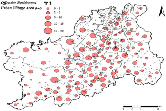
Figure 2.
Location of offender residences and urban villages in the study area.
2.2. Dependent Variable
In this study, the offender residences data, namely, the number of offender residences per grid cell, was taken as the dependent variable, which was provided by the Bureau of Public Security. The data included the residential addresses of offenders who lived, committed a crime, were arrested, and were sentenced in the study area in 2020. It did not include offenders who lived in the study area, but ones that committed crimes outside the study area. Due to the availability and privacy stipulations of the data, they did not specify the types of crimes committed. Examples of offender residence data are presented in Table 1 and contain information about the residential address, the arrest date of offenders in the study area, and the geocoding coordinate results based on the addresses (the last two fields). For the sake of data security, personal information (except residential address) was deleted before obtaining the data, including name and ID number. Moreover, also to protect privacy, the specific room numbers of the residential addresses were also removed by the provider, since most of the addresses were apartments or units in buildings rather than private single-family houses.

Table 1.
Examples of offender residence data.
The preprocessing of the offender residences data included two steps. First, the data with missing or incorrect text addresses were deleted. Second, the original addresses were geocoded to obtain the geocoordinates via the Baidu Map API. In this process, the coordinates of the offender residences were manually checked and corrected, and those with missing or incorrect geocoding results were removed. The raw data contained 3872 addresses, and the first step excluded 79 entries (2%), while the second step excluded 101 entries (2.6%). The filtered data contained 3692 pieces of data (95.4%). Therefore, in general, the amount of data after cleaning the accounts for a high proportion of the original data, and the data quality and accuracy were good enough for the later analysis.
2.3. Selection of Independent Variable
This study aimed to explore the association between offender residences and the urban built environment. Following related studies, we selected land use and socioeconomic facilities as independent variables, as listed in Table 2 [60,61,62,63,64,65]. First, points of interest (POI) data were obtained via Baidu Map API in 2020 that included nine types of places and facilities: factories, hotels, agricultural facilities, warehousing, entertainment facilities, IT companies, stores and malls, business-leasing service companies, and banks. Then, land use data were provided by the local land use bureau, from which the urban village data were extracted. Third, population data (the population count within a 500 m grid) was provided by the local mobile communication operator, which was calculated from cell phone data.
Table 2.
List of variables.
The social disorganization theory holds that a neighborhood with a high residential instability, low socioeconomic status, and high ethnic heterogeneity is likely to experience social disorder and higher crime rates as a result of low levels of social cohesion and social control [2,66,67,68,69,70]. The selection of independent variables in this study was based on the social disorganization theory and a similar study on offender residences in China [1]. The unique regional characteristics of the study area were also considered.
It is worth noting that urban villages in China have similar characteristics to those described in the explanation of the social disorganization theory mentioned above. Urban villages are an important factor in crime and offender residence research in a non-Western context, especially in China [1]. Therefore, urban village land use data were selected, which were extracted from the land use/cover data in the form of a polygon shapefile.
Among the nine types of POI places, POI data about shopping malls, hotels, banks, and entertainment facilities (including KTVs, bars, net bars, and massage parlors) have been tested as crime attractors and generators in previous related studies [16,17,18,65,66,67]. As defined by Brantingham and Brantingham, crime generators refer to places that attract large volumes of potential victims and, correspondingly, greater opportunities for crime [18]. Crime attractors refer to places known to be frequented by offenders that exhibit high levels of deviant behavior and generate extra opportunities for crime [18].
The socioeconomic status of neighborhoods is related to the residential choice of offenders [71]. Factories, agricultural facilities, and warehousing can be categorized as areas with a relatively low socioeconomic status, while IT companies and business-leasing service companies can be categorized as areas with a relatively high socioeconomic status. In this study, these two sets of POI were used to evaluate and compare the variations in the socioeconomic status in the study area.
Moreover, the population was also added as an independent variable [72,73].
3. Research Questions and Methodology
3.1. Research Questions and Hypotheses
This study aimed to answer three questions: (1) Where do offenders reside? (2) What is the individual association between each built environment factor and offenders’ residential locations? (3) What is the difference between the interactive associations of factors and the individual association between each factor and offender residences?
The social disorganization theory holds that a neighborhood with a high residential instability, low socioeconomic status, and high ethnic heterogeneity is likely to experience social disorder and even crime as a result of the low level of social cohesion and social control [2]. Based on this, our hypotheses were as follows: (1) A socially disorganized area characterized by a high residential instability, low socioeconomic status, and poor residential land use is the residential choice preference of offenders. (2) Due to the characteristics of the study area, urban villages may be an important factor with high explanatory power. (3) As demonstrated by Brantingham and Brantingham, crime generators refer to places that attract large volumes of potential victims and, correspondingly, large numbers of opportunities for crime [18]. Crime attractors refer to places known to be frequented by offenders that exhibit high levels of deviant behavior and that generate opportunities for crime [18]. Therefore, places that have many shopping malls, hotels, banks, and entertainment facilities (including KTVs, bars, net bars, and massage parlors) might be associated with offender residences, as they have been labeled as crime attractors and generators in previous related studies [65,66,67]. (4) The associations between the urban built environment and the residential locations of offenders are complicated and comprehensive. The explanatory power of interactive associations is beyond the association between any one individual factor and offender residences. Rather, interactive associations between factors might have a higher explanatory power.
3.2. Methodology
3.2.1. Preprocessing of Data
As mentioned in Section 2.3, 11 factors were selected as independent variables in this study to represent the ambient built environment in order explore its association with offender residences. Following the preprocessing of the GeoDetector modeling [74], first, a 500 × 500 m grid covering the study area was built via ArcGIS. Second, each type of POI data was counted within each grid, which was equal to the density of POIs since the grids were uniform in size. Then, the urban village area was calculated in each grid via ArcGIS. In this process, zero remained in grids without a variable data distribution. Finally, the dependent variable remained in the form of the numerical value. The 11 independent variables were then reclassified into six classes (from numerical to categorical data) by the natural breaks method in ArcGIS [57] (Figure 3).
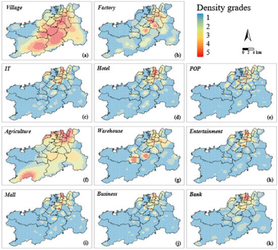
Figure 3.
Spatial distribution of potential factors: (a) urban village area; (b) density of factories; (c) density of IT companies; (d) density of hotels; (e) population density; (f) density of agriculture POIs; (g) density of warehouses; (h) density of entertainment places, including KTVs, net bars, and massage parlors; (i) density of shopping malls and stores; (j) density of business-leasing service POIs; (k) density of banks.
3.2.2. Kernel Density Estimation
KDE is a nonparametric method that uses a density estimation technique and has been widely adopted to reveal overall crime distributions and detect hot spots [42,43,44,45,46]. This method enables the observer to evaluate the local probability of whether an accident can occur and the degree of danger in a given zone [42]. In this study, the research object was offender residence, which was in the form of discrete location points. In analyzing the spatial distribution characteristic of offender residences, the KDE is an effective method to analyze and compare the spatial heterogeneity of offender residences. In this study, for a given set of offender residences observed from an unknown probability density function, we used the kernel estimator in a 2D space [42]; this estimator could be defined as follows:
where is the density at location , is the search radius of the kernel density estimation, is the number of sampling points, and is the weight of a point at the distance to location and is usually modeled as a kernel function of the ratio between and . In this study, we used the kernel with a Gaussian function, which could be formulated as follows:
3.2.3. Geographical Detectors Model
Related studies mainly applied various kinds of regression models regardless of the interactive associations of potential factors. Hence, to solve this problem, a new method was adopted in this study. The geographical detector (GeoDetector) model proposed by Wang et al. is a spatial heterogeneity detection method based on a spatial variance analysis [56]. It can be used to quantify the explanatory power of each factor on the dependent variable. GeoDetectors are a group of geographical statistical methods that detect spatial variability and reveal the factors behind it. Its calculation theory assumes that if an independent variable has an important association with a dependent variable, the spatial distribution of the independent variable and the dependent variable should be similar [56]. The consistency of the two spatial distributions of dependent variable y and independent variable x reflects the correlation of the two variables [56]. This correlation includes both linear and nonlinear parts, which can be measured with geographic detectors. The purpose of the linear regression model and the geographic detector is to establish the statistical association between the two variables in order to infer a possible causal association. In general, when the linear regression is significant, the geographic detector must be significant. If the linear regression is not significant, the geographic detector may still be significant. If the two variables are related, the geographic detector is capable of detecting them [57]. Due to the principles of the geographic detector model, it is not sensitive to collinearity [57]. In terms of the scale, the data preprocessing and modeling of the GeoDetector model are local processes based on spatial heterogeneity, while the detection results are global. Therefore, the GeoDetector model results were measured on a 500 × 500 m grid scale in this study.
The GeoDetector model is an open-source modeling software in the form of an Excel macro (http://geodetector.cn/, accessed on 1 March 2022). The basic process involves inputting the spatial statistics of the dependent and explanatory variables within spatial units in GIS software in order to output the attribute table into the GeoDetector Excel macro software to read the data and then run the model. Based on the power of the determinant, the GeoDetector model generates four detectors, including the factor detector, risk detector, ecological detector, and interactive detector [56]. Among them, the factor detector and interactive detector are more popular, and were also used in the study to explore the individual and interactive associations of determinants on the occupation mixture index distribution [56,57].
Specifically, the factor detector used the power of the determinant (termed ) [56] to quantify the impact of different factors on the spatial pattern of offender residences (Figure 4). As for factor , the value of could be calculated as [56]:
where refers to a study area that is divided into units, which is stratified into stratum [56]; and stratum consists of units. and denote the global variance of the dependent variable in the study area and the variance of the dependent variable in the subareas, respectively. Moreover, is the explanatory power index of the factors , [56]. When the value of is higher, the value of is closer to , which means that the explanatory power of the factor makes a stronger contribution to the occurrence of offender residences [56].
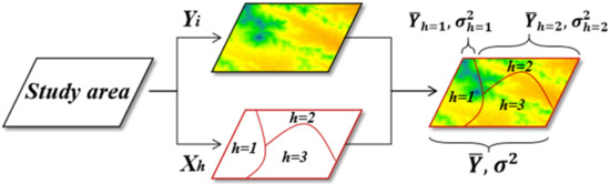
Figure 4.
The principle of the geographical detector.
Furthermore, the interaction detector was used to determine whether two individual factors enhance or weakened each other by comparing their combined contribution with their independent contributions (Figure 5). In short, the function of the interaction detector was to compare the difference between the individual associations of factors on the dependent variable and the interactive joint associations of two factors. The calculation and comparison process could be carried out as follows. For convenience, we denoted the explanatory power index of factor and as and , respectively. Additionally, the explanatory power of the interaction of these factors could be denoted as . The interaction between factors and depended on the association between and , , which could be categorized into five types [57], as shown in Table 3.
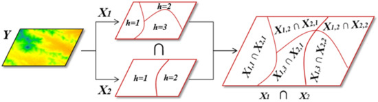
Figure 5.
The detection of interaction.
Table 3.
The interaction associations.
4. Results and Discussion
4.1. Portrait of Offenders
The characteristics of offenders, such as the gender and age structure (Figure 6), were some of the most important aspects of this study, and were helpful for understanding the internal diversity of this population in order to contribute to social management.
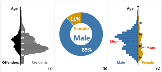
Figure 6.
The age structure of offenders and the total population (a), the gender structure of the offenders (b), and the age structure of female and male offenders (c).
There were 3692 offenders in the study area in 2020, among which most were middle-aged (with an average age of 43 years old) and male (with a male-to-female ratio of 9:1). The average ages of male and female offenders were 43 and 39 years, respectively. As shown in Figure 6a, the gender ratio of offenders varied greatly compared to that of the overall population.
4.2. Spatial Distribution of Offender Residences
Figure 7 shows the spatial distribution of offender residences. Overall, offender residence hot spots were mainly located in the middle of the study area. A polycentric structure could be observed within the standard deviation ellipse. The long-axis distribution direction of the standard deviation ellipse (southwest to northeast) showed that the overall spatial distribution of the offender residences in the study area tended to be consistent with the geometric shape of the study area boundary. The middle of the study area was located close to two transportation hubs, an airport and a railway station, with airport expressways passing through the region, developed transportation, and a large migrant population. Moreover, the area was a typical suburban region with many urban villages. This region had always been a high-incidence area regarding urban problems and provided offenders with space to hide.
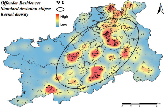
Figure 7.
Spatial distribution of offender residences.
4.3. Results of GeoDetector Model
4.3.1. Factor Detection
Taking the number of offender residential locations in each grid as the dependent variable and the 11 potential factors as the independent variables, the offender residence distribution was analyzed using the geographic detector model. The results obtained with the factor detector model are listed in Table 4. Theoretically, the range of the q value was 0–1, and the magnitude of the q value was through the comparison between factors. The larger the q value was, the stronger the explanatory power of the factor on the dependent variable.
Table 4.
Results of the factor detection. (Mean q value = 0.27).
As shown in Table 4, apart from the density of business-leasing service companies and the density of banks, the p values of the other nine factors were all less than 0.05, indicating that these nine factors had significant explanatory power on the spatial distribution of the offender residences at the significance level of 0.05. That stated, the model was suitable to explain the associations between the built environment and offender residences in this study.
The results showed that the density of factories, urban village area, and density of hotels were the three independent variables above the mean q value (0.27). That stated, as hypothesized, these three variables were key factors in terms of individual associations.
Second, the q value (0.39) of the urban village area ranked second after that of the density of factories. As hypothesized, it also indicated the relatively high explanatory power of urban villages on offender residences. Notably, urban villages in China do not refer to traditional villages. Urban villages are a peculiar phenomenon that has appeared in the process of urbanization in mainland China. In a narrow sense, urban villages refer to the evolution of residential areas from rural villages during the urbanization process as all or most of the cultivated land is expropriated, but farmers still live in the original villages after becoming residents. In a broad sense, urban villages refer to residential areas that lag behind the current development pace, drift away from modern urban management, and have maintained low living standards throughout the rapid urban development process. There is usually no unified planning or management within urban villages. The second highest q value of the urban village area reflected that offender residences were also highly reliant on urban villages, especially large urban villages. It has been demonstrated that urban villages in China are closely linked with a deteriorating social order and higher crime rates [75,76]. Furthermore, over 2.3 million nonlocal residents lived in the study area. Those migrants were often in a disadvantaged position in terms of wage and social welfare without a hukou in the city [77]. As a result of low income, urban villages are the popular residential choice for many migrants due to their low rent [78]. Due to the high mobility and instability of migrants, urban villages in Chinese cities are associated with a decline in public security and the deterioration of social order [75].
Third, the q value of the hotel (0.34) was also higher than the mean q value, ranking after the factory and village, which also indicated a relatively high explanatory power for offender residences. On the one hand, hotels are usually considered to be places that are prone to crime and attract crime [79,80,81]. As an economic facility, the hotel has commercial sensitivity and large internal population mobility, which is like a complex small society [79]. They naturally attract offenders and are considered to present inherent opportunities and convenience for criminal activities [80]. Related studies have confirmed that theft is the most common type of crime in hotels [81,82]. On the other hand, the residential choices of offenders usually depend on the proximity of potential victims [83]. The routine activity theory has also been applied to explain where offenders live, which emphasizes that most crimes occur due to the existence of possible offenders and appropriate targets, as well as the integration of incompetent guardians in time and space [84]. It should be noted that the POIs of various places were selected as the explanatory variable in this study in order to analyze the spatial associations between these places and offender residences from the perspective of spatial proximity. A possible explanation of the relatively high explanatory power of the hotel was that offender residences may be located close to the hotel, rather than the offenders living in hotels.
4.3.2. Interaction Detection
The interactive associations of factors on offender residences were investigated using the interaction detector model, and the results are shown in Table 5. The colored grids represent the interactive associations, and the grey grids represent the individual associations (factor detection). Firstly, the interactive associations of any two factors were quantified as a nonlinear enhancement, which was the most explanatory type of interaction. As hypothesized, it indicated that the interactive associations of every pair of factors on offender residences were more significant with a more powerful explanation than individual associations.
Table 5.
Results of interactive detector model. (The colored grids represent the interactive associations of factor pair, and the grey grids are the individual associations between single factor and offender residences, which is equal to the results of the factor detection.)
Importantly, we found that the interactions linked with urban village areas had the greatest joint associations, followed by interactions linked to the density of factories (highlighted in Table 5 in bold). It was, thus, confirmed again that urban villages and factories were essential factors when explaining the distribution of offender residence locations. Among 55 pairs of factors, the village ∩ hotel pair was the most explanatory pair of factors on offender residence. The results of the interaction detector proved that hotels located around urban villages (joint q value = 0.65) and entertainment places (joint q value = 0.58) especially increased the possibility of offender residences, which was consistent with the routine activity theory-based case that a neighborhood-built environment around the hotel reduced the security of the hotel and increased the possibility for crime [82]. Moreover, the interaction of village ∩ business ranked third with a joint q value of 0.57, also indicating a high interactive association. This was also consistent with and extended a study that found that commercial land use was positively associated with male delinquent residence [22].
4.4. Summary
Our research results mainly included two parts: factor detection and interaction detection. Firstly, the individual explanatory power of 11 built environment factors to the spatial distribution of offender residences was quantified. In this step, our results reached a depth similar to other studies using regression models. Then, in the second step, we quantified the interactive explanatory power of each pair of factors on the spatial distribution of offender residences, which was an extension of the relevant literature. For example, the results of interaction detection showed that the interactive explanatory power of the urban village and hotel on the spatial distribution of offender residences was 0.65, while that of the urban village and warehouse was 0.51. According to the principle of the GeoDetector model, the above results indicated that the urban village and hotel jointly explained 65% of the variance of the spatial distribution of offender residences, while the urban village and warehouse jointly explained 51% of the variance. It quantitatively indicated that within the scope of the urban village, the possibility of offender residences around the hotel was 14% higher than that around the warehouse.
The results of the study have the potential to identify areas prone to offender residences in order to make better decisions and suggestions regarding allocating crime prevention resources. For example, macroscopically speaking, for this study area, the urban village area was a hot area of offender residences. Microcosmically speaking, hotels, entertainment places, businesses, factories, and shopping malls within the scope of the urban villages were the places most closely related to offender residences.
Although this study did not obtain information about whether the offenders were migrants or not in offender residences data, the results of this study indicated that the urban village was the most important factor influencing the distribution of offender residences with a relatively high q value and joint q value. Therefore, the final focus of this study concerns the issue of the management of urban villages in Chinese cities. In the past three decades, there has been an unprecedented wave of migrant workers pouring into urban areas for employment in China. Due to their lack of hukou and low income, migrant workers are in a weak position in society, far away from their hometowns, and gather in urban villages to live and work. This has led to more and more urban villages with a weaker population stability and greater mobility, and urban villages in megacities in China are, thus, associated with decreased public safety and a deteriorating social order [76]. To address this issue, maintaining and standardizing rental housing and improving the quality of living environments in urban villages might be a solution [84], rather than eliminating urban villages [85]. In addition, by enhancing employment opportunities and community activities and other measures of multidepartment cooperation, we can promote the integration of potential migrant offenders in urban villages into local community life and improve the social neighborhood association between residents and immigrants in urban villages [1]. Promoting the gradual transformation of urban villages, including the built environment and internal residents, from “village” to “city” through multichannel and multidepartment cooperation might be an effective way to solve the problem of urban villages in China.
4.5. Limitations and Future Research
Despite its merits, this study had limitations that should be addressed in future studies. First, due to data availability, the offender residences data provided by public security departments were only the consolidated data that did not contain information on the specific types of crime the offenders committed. As we know, there is spatial heterogeneity in the spatial distribution of crime events and offender residences of different types of crime. Therefore, uncertainties existed in this study because we aimed to analyze the potential factors of all types of offender residences in the study area from a general perspective, rather than a specific type of offender. This study should be extended by obtaining more detailed data on the specific types of crimes committed.
Second, there was a possible sampling bias in the offender residence data, since the data used in this study only recorded the residential address of offenders who lived, committed crimes, were arrested, and were sentenced in the study area in 2020. However, these data did not include all offenders related to the study area; for example, those offenders who lived in the study area but committed crimes outside the study area were not included in the data due to data availability. In general, offenders related to the study area could be divided into three types: those who live and commit crimes in the study area, offenders who live in the study area but commit a crime outside the study area, and offenders who live outside the study area but commit a crime within the study area. However, this limitation might lead to overestimations, since only the first type of offender was considered in this study, and the reported associations were focused on those offenders who live and commit crimes within the study area.
Third, only offender residences were involved in this study. In the future, not only should we include the specific types of crimes committed, but we should also look at the address where crimes were committed to investigate the issue of journey-to-crime distance, which is also an important crime geography research issue [48]. Moreover, future studies should be extended by analyzing the variations between offenders and other residents in both spatial distribution and influencing factors, by which the distribution of offender residences can be explored and compared from more perspectives.
In addition, although this study primarily followed the social disorganization theory, future work should be extended by selecting more variables related to this theory, such as the number of migrants, percentage of rental residences, education degree, etc. [1], which were not considered in this study due to data availability. Moreover, although this study fully used the advantage of the geographical detector model in quantifying the interactive associations between factors based on the spatial analysis of variance, future work could be integrated with other methods such as geographical weight regression to further explore the spatially varying influences of factors on the dependent variable [86,87,88]. Apart from the association analysis, future studies should also focus on estimations of the most likely areas of offender residences by analyzing the locations of a connected series of crimes using geographic profiling [89] and space time pattern mining method [90].
5. Conclusions
Our empirical findings highlighted that the urban village was the most important factor in the associations between the urban built environment and offender residences. In general, taking the urban village as the carrier, various places (hotels, entertainment places, factories, business areas, and commercial areas) in the urban village had significant explanatory power on the location distribution of offender residences. This study enabled us to reflect on the applicability of the social disorganization theory in non-Western countries such as China. The results of factor detection and interactive detection are largely consistent with the theory of social disorganization as discussed above.
This study contributes to the literature by investigating the factors of offender residence locations from an interactive perspective. It was conducted in a non-Western context based on the social disorganization theory that originated from the Western countries [8,9,10]. This study indicated that the social disorganization theory is applicable to offender residence locations in the Chinese megacities [1]. This study is helpful for understanding the characteristics of the residential choices of offenders and quantifying the interactive associations of factors on offender residences.
Author Contributions
Conceptualization, Tao Wan and Buhai Shi; methodology, Tao Wan; software, Tao Wan; validation, Tao Wan and Buhai Shi; formal analysis, Tao Wan and Buhai Shi; investigation, Tao Wan and Buhai Shi; resources, Buhai Shi; data curation, Tao Wan; writing—original draft preparation, Tao Wan and Buhai Shi; writing—review and editing, Tao Wan and Buhai Shi; visualization, Tao Wan; supervision, Buhai Shi; project administration, Tao Wan and Buhai Shi; funding acquisition, Tao Wan and Buhai Shi. All authors have read and agreed to the published version of the manuscript.
Funding
This work was supported by the Natural Science Basic Research Project of Guangzhou (No. 202201010081).
Institutional Review Board Statement
Not applicable.
Informed Consent Statement
Not applicable.
Data Availability Statement
Not applicable.
Conflicts of Interest
The authors declare no conflict of interest.
References
- Liu, L.; Feng, J.; Ren, F.; Xiao, L. Examining the relationship between neighborhood environment and residential locations of juvenile and adult migrant burglars in China. Cities 2018, 82, 10–18. [Google Scholar] [CrossRef]
- Shaw, C.R.; McKay, H.D. Juvenile Delinquency and Urban Areas; University of Chicago Press: Chicago, IL, USA, 1942. [Google Scholar]
- Law, J.; Quick, M.; Chan, P. Open area and road density as land use indicators of young offender residential locations at the small-area level: A case study in Ontario, Canada. Urban Stud. 2016, 53, 1710–1726. [Google Scholar] [CrossRef]
- Grubesic, T.H.; Murray, A.T. Sex offender residency and spatial equity. Appl. Spat. Anal. Policy 2008, 1, 175–192. [Google Scholar] [CrossRef]
- Duwe, G. Residency restrictions and sex offender recidivism: Implications for public safety. Annotation 2009, 2, 6–8. [Google Scholar]
- Grubesic, T.H. Sex offender clusters. Appl. Geogr. 2010, 30, 2–18. [Google Scholar] [CrossRef]
- Johnson, S.D.; Summers, L. Testing ecological theories of offender spatial decision making using a discrete choice model. Crime Delinq. 2015, 61, 454–480. [Google Scholar] [CrossRef] [Green Version]
- Sampson, R.J.; Groves, W.B. Community structure and crime: Testing social-disorganization theory. Am. J. Sociol. 1989, 94, 774–802. [Google Scholar] [CrossRef] [Green Version]
- Law, J.; Quick, M. Exploring links between juvenile offenders and social disorganization at a large map scale: A Bayesian spatial modeling approach. J. Geogr. Syst. 2013, 15, 89–113. [Google Scholar] [CrossRef]
- Breetzke, G.D.; Horn, A.C. Crossing the racial divide: A spatial-ecological perspective of offenders in the City of Tshwane Metropolitan Municipality, South Africa. GeoJournal 2006, 67, 181–194. [Google Scholar] [CrossRef]
- Barbosa, G.Y. Immigrant residential segregation. In The Wiley Blackwell Encyclopedia of Urban and Regional Studies; Wiley: Hoboken, NJ, USA, 2019; pp. 1–9. [Google Scholar]
- King, R.D.; South, S.J. Crime, race, and the transition to marriage. J. Fam. Issues 2011, 32, 99–126. [Google Scholar] [CrossRef]
- South, S.J.; Messner, S.F. Crime and demography: Multiple linkages, reciprocal relations. Annu. Rev. Sociol. 2000, 26, 83–106. [Google Scholar] [CrossRef]
- Hirschman, C.; Tolnay, S.E. Social demography. In Handbook of Population; Springer: Boston, MA, USA, 2005; pp. 419–449. [Google Scholar]
- Cohen, L.E.; Felson, M. Social change and crime rate trends: A routine activity approach. In Classics in Environmental Criminology; Routledge: Oxfordshire, UK, 1979; pp. 588–608. [Google Scholar]
- Brantingham, P.L.; Brantingham, P.J. A theoretical model of crime hot spot generation. Stud. Crime Crime Prev. 1999, 8, 7–26. [Google Scholar]
- Brantingham, P.L.; Brantingham, P.J. Nodes, paths and edges: Considerations on the complexity of crime and the physical environment. J. Environ. Psychol. 1993, 13, 3–28. [Google Scholar] [CrossRef]
- Brantingham, P.J. Criminality of place: Crime generators and crime attractors. Eur. J. Crim. Policy Res. 1995, 3, 5–26. [Google Scholar] [CrossRef]
- Bernasco, W. A sentimental journey to crime: Effects of residential history on crime location choice. Criminology 2010, 48, 389–416. [Google Scholar] [CrossRef]
- Mustaine, E.E.; Tewksbury, R.; Stengel, K.M. Residential location and mobility of registered sex offenders. Am. J. Crim. Justice 2006, 30, 177–192. [Google Scholar] [CrossRef]
- Tewksbury, R.; Mustaine, E.E. Where registered sex offenders live: Community characteristics and proximity to possible victims. Vict. Offenders 2008, 3, 86–98. [Google Scholar] [CrossRef]
- Wallis, C.P.; Maliphant, R. Delinquent areas in the county of London: Ecological factors. Br. J. Criminol. 1967, 7, 250–284. [Google Scholar] [CrossRef]
- Roncek, D.W.; Bell, R. Bars, blocks, and crimes. J. Environ. Syst. 1981, 11, 35–47. [Google Scholar] [CrossRef]
- McCord, E.S.; Ratcliffe, J.H. Intensity value analysis and the criminogenic effects of land use features on local crime patterns. Crime Patterns Anal. 2009, 2, 17–30. [Google Scholar]
- Felson, M.; de Melo, S.N.; Boivin, R. Risk of outdoor rape and proximity to bus stops, bars, and residences. Violence Vict. 2022, 36, 723–738. [Google Scholar]
- Hart, T.C.; Miethe, T.D. Street robbery and public bus stops: A case study of activity nodes and situational risk. Secur. J. 2014, 27, 180–193. [Google Scholar] [CrossRef]
- Caplan, J.M.; Kennedy, L.W.; Miller, J. Risk terrain modeling: Brokering criminological theory and GIS methods for crime forecasting. Justice Q. 2011, 28, 360–381. [Google Scholar] [CrossRef]
- Drawve, G. A metric comparison of predictive hot spot techniques and RTM. Justice Q. 2016, 33, 369–397. [Google Scholar] [CrossRef]
- Drawve, G.; Moak, S.C.; Berthelot, E.R. Predictability of gun crimes: A comparison of hot spot and risk terrain modelling techniques. Polic. Soc. 2016, 26, 312–331. [Google Scholar] [CrossRef]
- Connealy, N.T.; Piza, E.L. Risk factor and high-risk place variations across different robbery targets in Denver, Colorado. J. Crim. Justice 2019, 60, 47–56. [Google Scholar] [CrossRef]
- Adeyemi, R.A.; Mayaki, J.; Zewotir, T.T.; Ramroop, S. Demography and crime: A spatial analysis of geographical patterns and risk factors of Crimes in Nigeria. Spat. Stat. 2021, 41, 100485. [Google Scholar] [CrossRef]
- Sherman, L.W.; Gartin, P.R.; Buerger, M.E. Hot spots of predatory crime: Routine activities and the criminology of place. Criminology 1989, 27, 27–56. [Google Scholar] [CrossRef]
- Eck, J.; Chainey, S.; Cameron, J.; Wilson, R. Mapping Crime: Understanding Hotspots; U.S. Department of Justice Office of Justice Programs: Washington, DC, USA, 2005. [Google Scholar]
- Hart, T.C. Investigating crime pattern stability at micro-temporal intervals: Implications for crime analysis and hotspot policing strategies. Crim. Justice Rev. 2021, 46, 173–189. [Google Scholar] [CrossRef]
- Mondal, S.; Singh, D.; Kumar, R. Crime hotspot detection using statistical and geospatial methods: A case study of Pune City, Maharashtra, India. GeoJournal 2022, 1–17. [Google Scholar] [CrossRef]
- Hodgkinson, T.; Andresen, M.A. Changing spatial patterns of residential burglary and the crime drop: The need for spatial data signatures. J. Crim. Justice 2019, 61, 90–100. [Google Scholar] [CrossRef]
- Zhao, X.; Tang, J. Modeling temporal-spatial correlations for crime prediction. In Proceedings of the 2017 ACM on Conference on Information and Knowledge Management, Singapore, 6–10 November 2017; pp. 497–506. [Google Scholar]
- Piza, E.L.; Carter, J.G. Predicting initiator and near repeat events in spatiotemporal crime patterns: An analysis of residential burglary and motor vehicle theft. Justice Q. 2018, 35, 842–870. [Google Scholar] [CrossRef]
- Yang, B.; Liu, L.; Lan, M.; Wang, Z.; Zhou, H.; Yu, H. A spatio-temporal method for crime prediction using historical crime data and transitional zones identified from nightlight imagery. Int. J. Geogr. Inf. Sci. 2020, 34, 1740–1764. [Google Scholar] [CrossRef]
- Brownstein, J.S.; Green, T.C.; Cassidy, T.A.; Butler, S.F. Geographic information systems and pharmacoepidemiology: Using spatial cluster detection to monitor local patterns of prescription opioid abuse. Pharmacoepidemiol. Drug Saf. 2010, 19, 627–637. [Google Scholar] [CrossRef] [Green Version]
- Joshi, A.; Sabitha, A.S.; Choudhury, T. Crime analysis using K-means clustering. In Proceedings of the 2017 3rd International Conference on Computational Intelligence and Networks (CINE), Odisha, India, 28 October 2017; pp. 33–39. [Google Scholar]
- Kalinic, M.; Krisp, J.M. Kernel density estimation (KDE) vs. hot-spot analysis—Detecting criminal hot spots in the City of San Francisco. In Proceedings of the 21st Conference on Geo-Information Science, Lund, Sweden, 12–15 June 2018. [Google Scholar]
- Mburu, L.W.; Zipf, A. A Spatial Approach to Surveying Crime—Problematic Areas at the Street Level. In Connecting a Digital Europe Through Location and Place; Springer: Berlin/Heidelberg, Germany, 2014. [Google Scholar]
- Levine, N. Crimestat IV: A Spatial Statistics Program for the Analysis of Crime Incident Locations, Version 4.0; Ned Levine & Associates: Houston, TX, USA, 2013. [Google Scholar]
- Chainey, S.; Ratcliffe, J. Identifying crime hotspots. In GIS and Crime Mapping; John Wiley & Sons: Hoboken, NJ, USA, 2005; pp. 145–182. [Google Scholar]
- Ratcliffe, J. Crime mapping: Spatial and temporal challenges. In Handbook of Quantitative Criminology; Springer: New York, NY, USA, 2010; pp. 5–24. [Google Scholar]
- Chainey, S.P. Examining the influence of cell size and bandwidth size on kernel density estimation crime hotspot maps for predicting spatial patterns of crime. Bull. Geogr. Soc. Liege 2013, 60, 7–19. [Google Scholar]
- Hart, T.; Zandbergen, P. Kernel density estimation and hotspot mapping: Examining the influence of interpolation method, grid cell size, and bandwidth on crime forecasting. Polic. Int. J. Police Strateg. Manag. 2014, 37, 305–323. [Google Scholar] [CrossRef]
- Xiao, L.; Liu, L.; Song, G.; Ruiter, S.; Zhou, S. Journey-to-crime distances of residential burglars in China disentangled: Origin and destination effects. ISPRS Int. J. Geo-Inf. 2018, 7, 325. [Google Scholar] [CrossRef] [Green Version]
- Browning, C.R.; Byron, R.A.; Calder, C.A.; Krivo, L.J.; Kwan, M.P.; Lee, J.Y.; Peterson, R.D. Commercial density, residential concentration, and crime: Land use patterns and violence in neighborhood context. J. Res. Crime Delinq. 2010, 47, 329–357. [Google Scholar] [CrossRef]
- Xia, Z.; Stewart, K.; Fan, J. Incorporating space and time into random forest models for analyzing geospatial patterns of drug-related crime incidents in a major us metropolitan area. Comput. Environ. Urban Syst. 2021, 87, 101599. [Google Scholar] [CrossRef]
- LeSage, J.; Pace, R.K. Introduction to Spatial Econometrics; Chapman and Hall: London, UK, 2009. [Google Scholar]
- Chen, J.; Liu, L.; Liu, H.; Long, D.; Xu, C.; Zhou, H. The Spatial Heterogeneity of Factors of Drug Dealing: A Case Study from ZG, China. ISPRS Int. J. Geo-Inf. 2020, 9, 205. [Google Scholar] [CrossRef] [Green Version]
- Chen, J.; Liu, L.; Zhou, S.; Xiao, L.; Song, G.; Ren, F. Modeling spatial effect in residential burglary: A case study from ZG city, China. ISPRS Int. J. Geo-Inf. 2017, 6, 138. [Google Scholar] [CrossRef] [Green Version]
- Chen, J.; Liu, L.; Xiao, L.; Xu, C.; Long, D. Integrative analysis of spatial heterogeneity and overdispersion of crime with a geographically weighted negative binomial model. ISPRS Int. J. Geo-Inf. 2020, 9, 60. [Google Scholar] [CrossRef] [Green Version]
- Wang, J.F.; Li, X.H.; Christakos, G.; Liao, Y.L.; Zhang, T.; Gu, X.; Zheng, X.Y. Geographical detectors-based health risk assessment and its application in the neural tube defects study of the Heshun Region, China. Int. J. Geogr. Inf. Sci. 2010, 24, 107–127. [Google Scholar] [CrossRef]
- Wang, J.; Zhang, T.; Fu, B. A measure of spatial stratified heterogeneity. Ecol. Indic. 2016, 67, 250–256. [Google Scholar] [CrossRef]
- Weisburd, D.; Groff, E.R.; Yang, S.M. The Criminology of Place: Street Segments and our Understanding of the Crime Problem; Oxford University Press: Oxford, UK, 2012. [Google Scholar]
- Shaw, C.R.; McKay, H.D. Juvenile delinquency and urban areas: A study of rates of delinquency in relation to differential characteristics of local communities in American cities (1969). In Classics in Environmental Criminology; Routledge: Oxfordshire, UK, 2010; pp. 103–140. [Google Scholar]
- Wang, Z.; Liu, L.; Zhou, H.; Lan, M. How is the confidentiality of crime locations affected by parameters in kernel density estimation? ISPRS Int. J. Geo-Inf. 2019, 8, 544. [Google Scholar] [CrossRef] [Green Version]
- Chainey, S.; Tompson, L.; Uhlig, S. The utility of hotspot mapping for predicting spatial patterns of crime. Secur. J. 2008, 21, 4–28. [Google Scholar] [CrossRef]
- Manepalli, U.R.; Bham, G.H.; Kandada, S. Evaluation of hotspots identification using kernel density estimation (K) and Getis-Ord (Gi*) on I-630. In Proceedings of the 3rd International Conference on Road Safety and Simulation, Indianapolis, IN, USA, 14–16 September 2011. [Google Scholar]
- Xie, Z.; Yan, J. Kernel density estimation of traffic accidents in a network space. Comput. Environ. Urban Syst. 2008, 32, 396–406. [Google Scholar] [CrossRef] [Green Version]
- Ihlanfeldt, K.R. Rail transit and neighborhood crime: The case of Atlanta, Georgia. South Econ. J. 2003, 70, 273–294. [Google Scholar] [CrossRef]
- Xu, C.; Chen, X.; Liu, L.; Lan, M.; Chen, D. Assessing Impacts of New Subway Stations on Urban Thefts in the Sur-rounding Areas. ISPRS Int. J. Geo-Inf. 2021, 10, 632. [Google Scholar] [CrossRef]
- Willits, D.; Broidy, L.; Denman, K. Schools, Neighborhood Risk Factors, and Crime. Crime Delinq. 2013, 59, 292–315. [Google Scholar] [CrossRef]
- Murray, R.K.; Swatt, M.L. Disaggregating the Relationship Between Schools and Crime: A Spatial Analysis. Crime Delinq. 2013, 59, 163–190. [Google Scholar] [CrossRef]
- Bursik, R.J. Social disorganization and theories of crime and delinquency: Problems and prospects. Criminology 1988, 26, 519–552. [Google Scholar] [CrossRef]
- Bursik, R.J.; Webb, J. Community Change and Patterns of Delinquency. Am. J. Soc. 1982, 88, 24–42. [Google Scholar] [CrossRef]
- Shaw, C.R. A Delinquency Area; Behavior Research Fund Monographs; Moore, M.E., Ed.; University of Chicago Press: Chicago, IL, USA, 1931; pp. 13–25. [Google Scholar]
- Hesseling, R.B.P. Using data on offender mobility in ecological research. J. Quant. Criminol. 1992, 8, 95–112. [Google Scholar] [CrossRef]
- Zhang, X.; Gao, F.; Liao, S.; Zhou, F.; Cai, G.; Li, S. Portraying Citizens’ Occupations and Assessing Urban Occupation Mixture with Mobile Phone Data: A Novel Spatiotemporal Analytical Framework. ISPRS Int. J. Geo-Inf. 2021, 10, 392. [Google Scholar] [CrossRef]
- Deng, X.; Liu, Y.; Gao, F.; Liao, S.; Zhou, F.; Cai, G. Spatial Distribution and Mechanism of Urban Occupation Mix-ture in Guangzhou: An Optimized GeoDetector-Based Index to Compare Individual and Interactive Effects. ISPRS Int. J. Geo-Inf. 2021, 10, 659. [Google Scholar] [CrossRef]
- Gao, F.; Li, S.; Tan, Z.; Wu, Z.; Zhang, X.; Huang, G.; Huang, Z. Understanding the modifiable areal unit problem in dockless bike sharing usage and exploring the interactive effects of built environment factors. Int. J. Geogr. Inf. Sci. 2021, 35, 1–21. [Google Scholar] [CrossRef]
- Song, Y.; Zenou, Y.; Ding, C. Let’s not throw the baby out with the bath water: The role of urban villages in housing rural migrants in China. Urban Stud. 2008, 45, 313–330. [Google Scholar] [CrossRef] [Green Version]
- Zhang, L.; Zhao, S.X.B.; Tian, J.P. Self-help in housing and Chengzhongcun in China’s urbanization. Int. J. Urban Reg. Res. 2003, 27, 912–937. [Google Scholar] [CrossRef]
- Wang, Y.P.; Wang, Y.; Wu, J. Housing migrant workers in rapidly urbanizing regions: A study of the Chinese model in Shenzhen. Hous. Stud. 2010, 25, 83–100. [Google Scholar] [CrossRef]
- Cheng, Z.; Guo, F.; Hugo, G.; Yuan, X. Employment and wage discrimination in the Chinese cities: A comparative study of migrants and locals. Habitat Int. 2013, 39, 246–255. [Google Scholar] [CrossRef]
- Kemshall, H. Sleep safely: Crime risks may be smaller than you think. Soc. Policy Adm. 2010, 31, 247–259. [Google Scholar] [CrossRef]
- Ho, T.; Zhao, J.; Brown, M.P. Examining hotel crimes from police crime reports. Crime Prev. Community Saf. 2009, 11, 21–33. [Google Scholar] [CrossRef]
- Harper, D.W.J. Comparing tourists crime victimization. Ann. Tour. Res. 2001, 28, 1053–1056. [Google Scholar] [CrossRef]
- Kelly, I. Tourist destination crime rates: An examination of Cairns and the Gold Coast, Australia. J. Tour. Stud. 1993, 4, 2–11. [Google Scholar]
- Steven, S. Social Structure and Swedish Crime Rates A Time-Series Analysis, 1950–1979. Criminology 2006, 20, 499–514. [Google Scholar] [CrossRef]
- Wei, L.; Yan, X. Transformation of ‘urban village’ and feasible mode. City Plan. Rev. 2005, 7, 9–13. [Google Scholar]
- Zheng, S.; Long, F.; Fan, C.C.; Gu, Y. Urban villages in China: A 2008 survey of migrant settlements in Beijing. Eurasian Geogr. Econ. 2009, 50, 425–446. [Google Scholar] [CrossRef] [Green Version]
- Gao, F.; Li, S.; Tan, Z.; Zhang, X.; Lai, Z.; Tan, Z. How Is Urban Greenness Spatially Associated with Dockless Bike Sharing Usage on Weekdays, Weekends, and Holidays? ISPRS Int. J. Geo-Inf. 2021, 10, 238. [Google Scholar] [CrossRef]
- Li, S.; Lyu, D.; Huang, G.; Zhang, X.; Gao, F.; Chen, Y.; Liu, X. Spatially varying impacts of built environment factors on rail transit ridership at station level: A case study in Guangzhou, China. J. Transp. Geogr. 2017, 82, 102631. [Google Scholar] [CrossRef]
- Fotheringham, A.S.; Charlton, M.E.; Brunsdon, C. Geographically weighted regression: A natural evolution of the expansion method for spatial data analysis. Environ. Plan. A 1998, 30, 1905–1927. [Google Scholar] [CrossRef]
- Rossmo, D.K. Geographic Profiling, 1st ed.; Routledge: Oxfordshire, UK, 1999. [Google Scholar] [CrossRef]
- Gao, F.; Li, S.; Tan, Z.; Liao, S. Visualizing the spatiotemporal characteristics of Dockless bike sharing usage in Shenzhen, China. J. Geovis. Spat. Anal. 2022, 6, 12. [Google Scholar] [CrossRef]

Publisher’s Note: MDPI stays neutral with regard to jurisdictional claims in published maps and institutional affiliations. |
© 2022 by the authors. Licensee MDPI, Basel, Switzerland. This article is an open access article distributed under the terms and conditions of the Creative Commons Attribution (CC BY) license (https://creativecommons.org/licenses/by/4.0/).