Abstract
This paper proposes to identify the variation of accessibility to healthcare facilities based on vulnerability assessments of floods by using open source data. The open source data comprises Open Street Map (OSM), world population, and statistical data. The accessibility analysis is more focused on vulnerable populations that might be affected by floods. Therefore, a vulnerability assessment is conducted beforehand to identify the location where the vulnerable population is located. A before and after scenario of floods is applied to evaluate the changes of healthcare accessibility. A GIS Network Analyst is chosen as the accessibility analysis tool. The results indicate that the most vulnerable population lives in the Asemrowo district. The service area analysis showed that 94% of the West of Surabaya was well-serviced in the before scenario. Otherwise, the decrement of service area occurs at the city center in the after scenario. Thus, the disaster manager can understand which vulnerable area is to be more prioritized in the evacuation process.
1. Introduction
FEMA (Federal Emergency Management Agency) classifies emergency management into four phases composed of mitigation, preparedness, response, and recovery [1]. The response is the most important phase of disaster management since it deals with necessary actions to address the immediate and short-term effects of the disaster, and to support life preservation and the basic subsistence needs of affected people [2]. The purposes of the response are saving lives, minimizing property damages, taking care of human needs, as well as anticipating the effect of upcoming disasters [3]. Huder [4] categorizes the response phase into four mechanisms comprising impact, stabilization, sustainment, and recovery. Urgency, impact, and stabilization are the key actions of the response phase. Impact and stabilization focus on life safety such as searching for and rescuing the victims, caring for the injured, and identification of the dead. Therefore, the preparedness of the evacuation plan is essential for reacting to the emergencies of disaster impact.
The phenomenon of flooding is common in Indonesia, especially during the peak period of the rainy season. According to the Meteorological, Climatological, Geophysical Agency of Indonesia (BMKG) report, January to March 2019 was the peak period of the rainy season, during which there was a rising impact of potential hydro-meteorological disasters such as floods [5]. The impacts caused after the hydro-meteorological disasters are diverse, including not only material losses e.g., public facility and property losses, but also non-material losses, e.g., deaths, injuries, and the spread of disease.
Geographic Information Systems (GIS) are a prompt solution for disaster management that supports the collecting, modeling, analyzing, and visualizing of disaster-related data [6]. In practice, GIS have become a standard tool for presenting multi-hazard and risk information using various forms of spatial visualization [7]. Taramelli et.al have proven that GIS applications are able to identify hazard potential and the elements at risk, and to reduce the impact of upcoming disasters by integrating different domains of data [8]. The utilization of GIS is not only applied to risk assessments but also in response and mitigation mapping for resilience and surveillance [9]. For instance, in the response process, ref. [10] presented the use of GIS analysis for identifying mammography availability. In their study, they used accessibility as the parameter for the purposes of routing from the geocodes of mammography facilities to incidental residents. In addition to the mitigation process, GIS is utilized for planning the location of new settlement areas by evaluating the resilience of existing settlements and calculating the suitability of new settlements [11]. Moreover, the capabilities of GIS have evolved to include sophisticated technologies in collecting and distributing necessary data from different domains [12] and real-time applications to promote the decision-making process [13], in which real-time GIS is embedded by dynamic data sources and sensors to monitor the actual conditions of the environment [14].
The healthcare service center is one of the supporting infrastructures in response activities, including hospitals and clinics [15]. In flood situations, hospitals and clinics not only take care of the ill and injured but also serve as a shelter to help in managing the homeless [16]. Hence, information on accessible healthcare is quite necessary for people in need [17] and disaster managers to proceed with the evacuation process. The optimization of the evacuation process relies on the improvement of accessibility in the vulnerable areas of the flood in which the victims are predominantly located [18]. Furthermore, access optimization is not only concerned with recovering the infrastructure damages but also seeking routes for the evacuation process [4,19]. However, due to the disaster-induced disruption, i.e., damaged infrastructure and hazard materials, healthcare accessibility must suffer negative effects.
Many studies have analyzed healthcare accessibility in a disaster situation. In a disaster situation, healthcare accessibility relies on the supply and demand information for optimizing spatial variations [17,20]. In this context, the supply is the healthcare center’s capacity, and the demand is the number of patients. Both have key roles in optimizing healthcare accessibility. As has been proposed by Chu et.al, the developed method called 3SFCA successfully minimized the spatial accessibility of dengue outbreaks based on temporal patients’ information [20]. Once the distribution of patients’ locations has been clustered, the accessibility would be more effective as the priorities have been identified accordingly [21]. In addition, the distribution of critical healthcare facility locations can ease in identifying the preferable destination for robust accessibility in post-disaster situations [22,23]. In the accessibility analysis, demand and supply become origins, and destinations are connected by links and costs. The links are road networks while the costs are time, distance, and fare. Rather than distance and fare, time becomes a crucial factor for accessibility in disaster situations [24]. Therefore, the accessibility analysis requires a method that is time-based to minimize the travel time and avoid the road network’s disruption.
Accessibility analysis can be generated either through vector-based or raster-based methods. Generally, vector-based accessibility can be measured by a straight line [25]. For instance, a buffer in the proximity analysis is used to identify the area that is accessible from a road network based on Euclidean distance, meaning that distance is generally calculated ignoring the road surface, path, road class, and travel time. Other researchers conducted an accessibility analysis considering travel costs. For example, Guth et.al. presented the use of fuzzy logic for estimating the average speed of road networks based on the parameter of road class, road slope, road surface, and link length [26]. They found that fuzzy logic is capable of obtaining the best results in distributing average speed even if the range of speed values was dispersed. Another approach was presented in [27], in which the researcher used Dijkstra’s algorithms to solve route problems by providing the shortest path for emergency management. The results proved that the Dijkstra algorithm embedded in network analysis is capable of modeling time variations derived from traffic count and improving travel times compared to static networks. The network analysis builds a road network dataset based on a geo-database of road data that is equipped with evaluator settings such as travel time, length, road hierarchy, and restriction [28,29]. Hence, network analysis has been more effectively implemented for routing purposes than straight line distance measurements.
Open source data is an alternative solution for data acquisition and replaces government data that is not freely available at large. However, the quality and quantity of the open-source dataset must be validated before the application. The quality of the dataset was assessed considering geometric accuracy, attribute accuracy, logical consistency, semantic accuracy, actuality, lineage, and usage [30], while the quantity of the dataset was assessed considering completeness and infrastructure-associated point datasets [31]. In other words, the assessment was carried out based on the actual real-world conditions from ground data. The applications of open source data have emerged for many purposes such as OSM data for routing analysis [26], population data for disaster response [32], and statistical data for analyzing the trend of virus outbreaks [33].
A similar study used GIS, particularly a network analysis of healthcare accessibility variation to investigate the un-serviced area and the size of the population that was covered by serviced areas in Jeddah City [17]. Another study concerning the use of GIS for supporting disaster response was conducted by Zhao et.al [34] and Chen et.al [35], who used time-varying shelter demands based on points of interest (POI) in China as the input in a location-allocation analysis to determine proper shelters for evacuees. Yao et.al [36] also analyze shelter demands in Canada; however, the destination shelter focused on the open space identification such as school playgrounds, squares, and green spaces. These open spaces were applied as the inputs in a flood evacuation simulation using OD Cost Matrix in GIS. The network analysis was generally implemented for disaster response and healthcare services. However, the demands were not produced by a risk analysis beforehand. In other words, the priority of demands was not assessed before applying the GIS network analysis.
Therefore, this research aims to implement GIS technologies for emergency response analysis in a flood situation. This research aims to assess the priority of the demand population by using vulnerability analysis and to generate the accessibility of nearby healthcare services by using GIS network analysis. The vulnerability assessment is carried out to identify people as the possible demand source and to investigate the number of facilities at risk to possible transportation disruptions in a post-disaster situation. Considering the land-use changes in Surabaya that have quickly occurred, this research chooses healthcare centers instead of identifying an open space area as the shelter. Furthermore, the accessibility analysis generates a spatial variation of the healthcare service area and produces a simulation of evacuation routes. To enhance safety and minimize drive-time and distance cost in action, this research simulates the flood situation based on a simulation scenario comprising before and after a flood.
2. Materials and Methods
2.1. Study Area
The study area is situated in the west of Surabaya, Surabaya, Indonesia (Figure 1). Surabaya is one of the important urban centers in Indonesia with a total area of 326.81 km². The administrative area is divided into 31 districts grouped on 4 territorial boundaries: west, east, north, and south. As the second metropolitan area in Indonesia after Jakarta, the population living in Surabaya accounted for around 2 million. Surabaya is situated in East Java Province, adjacent to the Madura Strait; consequently, Surabaya is a coastal area with an average altitude of 7.42 m above sea level [37]. In addition, based on Meteorology, Climate, Geophysics Agency (BMKG) data, Surabaya’s climate is categorized into a seasonal zone with a rainy season periodically occurring from October to March [5]. The average precipitation index reported in the rainy season is 200–300 mm/day. Consequently, a flood often occurs in critical areas of Surabaya such as Sukomanunggal, Benowo, Tandes, Asemrowo, Lakarsantri, and Sambikerep.
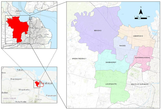
Figure 1.
Study area.
2.2. Dataset
Based on flood inundation simulations derived from Landsat 8 [38], this research conducts impact analysis to identify people and public facilities at risk. The impact analysis of people at risk was based on Surabaya’s population density collected from open spatial demographic data and research that is available in a raster format with a grid-based population number estimation of 100 m. This data was produced using a random forest technique and ancillary data to produce finer-scale patterns of population distribution [39,40]. The spatial scale of the grid is expected to represent the distribution of populations in the urban area.
In addition, population statistical data was collected from the Central Bureau of Statistics of Surabaya (BPS). Meanwhile, to identify infrastructure and healthcare facilities at risk, the data was collected from the Indonesia Geospatial Web portal managed by the Geospatial Information Agency of Indonesia (BIG) [41]. The impact analysis proceeded to be vector-based using ArcGIS software. Hence, all raster datatypes were vectorized beforehand.
To proceed with the network analysis, this research collected a large set of 2019 road network data from Open Street Map (OSM). The dataset contained some informative attributes, such as road class, road name, one-way information, road surface, and road length. Then, the OSM attribute was equipped with the average speed of vehicles and drive-time based on field surveys in each road class.
2.3. Flood Inundation Map
The flood inundation map was extracted from a spectral analysis of Landsat 8 satellite imagery using spectral algorithms for two indices: the Modified Normalized Water Index (MNDWI) and Normalized Difference Build-up Index (NDBI). The MNDWI is calculated based on the reflectance of green bands to recognize permanent water objects such as pond areas, rivers and pools, and the reflectance of Mid Infrared (MIR) bands to eliminate non-water objects including vegetation and build-up areas [42]. Meanwhile, the NDBI is calculated to optimize the reflectance of MIR bands to identify built-up areas and to minimize Near Infrared (NIR) bands to discriminate vegetation and water objects [43]. This research compares these spectral indices of temporal satellite imageries that are acquired in dry and rainy seasons to identify the potential of flood inundation.
MNDWI = (Green − MIR)/(Green + MIR),
NDBI = (MIR − NIR)/(MIR + NIR),
Thenceforth, the potential of flood inundation (PFI) is calculated using intersect analysis (Equation (3)), by optimizing the value of MNDWI and minimizing the value of NDBI both before and after flood incidents. Furthermore, the result of this calculation is validated by a flood distribution map of Surabaya produced by the Regional Disaster Management Agency.
2.4. Vulnerability Assessment
Vulnerability is defined as the characteristics and conditions comprising physical, social, economic, and environmental factors or processes that determine the susceptibility degree of a community to the damaging impact of hazards [44]. Vulnerability is one of the fundamental elements of risk assessment apart from hazard and capacity. Vulnerability is also addressed as elements at risk including exposure and community [45], in which risk is represented as a combination between the probability of events and its negative impact [44]. In this research, vulnerability assessment focuses on the social vulnerability. It is carried out to determine number of populations at risk based on the probability of flood events.
Before assessing the vulnerability, this research conducted a preliminary analysis of flood inundation in the study area. The results visualized inundation areas and flood potential impact. With respect to the inundation area, impact analysis was carried out to determine the potential impacted area, damaged infrastructures (consist of roads and bridges), impacted healthcare as exposure, and the population at risk. The present study divides the vulnerable assessment into two steps: (1) Identifying impacted areas and (2) vulnerability scoring as depicted in Figure 2.
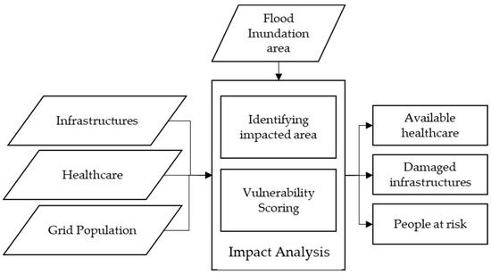
Figure 2.
Impact analysis procedure.
Vulnerability scoring (V) is calculated by Equation (4). It generates the number of people at risk based on some indicators comprising the gender ratio, the percentage of elderly and children, and population density.
where n is the number of indicators; is the value of each indicator, and is the weight of each indicator (60% for population density and 40% for gender ratio, elderly, and children). The weight is determined following the regulation of The National Agency for Disaster Countermeasure of Indonesia (BNPB) [46]. However, before applying the Equation (4), the normalization is carried out for the indicators to limit the range of vulnerability values. The normalization is calculated by Equation (5). Different methods are applied before the normalization process: (a) the value of the indicator in percentages is acquired by dividing the number of elderly and children by total population, (b) for population density, the values are transferred to percentages to equalize the value. The result of V is between 0–100 before the normalization process. Furthermore, the result of normalized V must be between 0–1.
where x is the value of each indicator, x min is the minimum value of indicators, and x max is the maximum value of indicators.
y = (x − x min)/(x max − x min),
2.5. Network Analysis
Network analysis solves a linear network as a constellation of nodes and connecting links such as roads, rivers, and railways [47]. The analysis is based on the Dijkstra algorithm to calculate distances between nodes and points in the network dataset. Ref. [48] describes the Dijkstra algorithm as an n-order simple weighted graph to analyze the shortest path from p to q by setting the weight to = ∞. Generally, this analysis is also developed by ESRI for routing purposes such as finding the fastest and closest path from incident to facility, calculating service area, and fleet routing problem, origin destination cost matrix, as well as location-allocation. The network analysis solves the routing problem based on the network dataset () that has been established beforehand. Sequentially, some relevant network attributes must be set as network dataset attributes , since the attributes are the evaluators in the network analysis process.
Figure 3 illustrates the network analysis procedure. The present study divides the network analysis procedure into three major steps: (1) Building network datasets; (2) performing service area analysis of healthcare based on the flood situation; (3) simulating evacuation routes. However, network analysis requires additional details before establishing a road network dataset such as drive-time and average vehicle speed. Therefore, a preliminary survey was carried out beforehand to collect the average speed in every road class. The road class represents a hierarchical sequence consisting of:
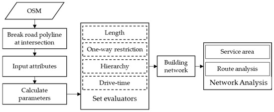
Figure 3.
Network Analysis Procedure.
- 1 = Motorway;
- 2 = Trunk;
- 3 = Primary;
- 4 = Secondary;
- 5 = Tertiary;
- 6 = Residential;
- 7 = Unclassified
After conducting a ground sampling on every road type, a network dataset is built by setting up some evaluators beforehand:
- Determine one-way restriction rules (IF ([DIR] = “1”) THEN True, ELSE IF False), “1” represents one-way that is restricted, and “0” represents vice versa.
- Determine length as cost (km), which is based on the cumulative length of each road edge following each road name based on the record of length attribute
- Calculate drive-time as cost in minutes based on Equation (6).where s = length (km), v = speed average of vehicle (km/h), and t = drive-time (min).t = s/v × 60,
- Determine the hierarchical priority of road class.
Service area analysis traverses the accessible street following the geometry of the street in accordance with the applied impedance, either time or length. The output of this analysis is a delineated region based on the range of impedance. In this research, a service area analysis is performed to identify the range of healthcare locations based on drive-time (Figure 4). In this analysis, some solved evaluators are determined. The following steps describe how service area analysis is applied:
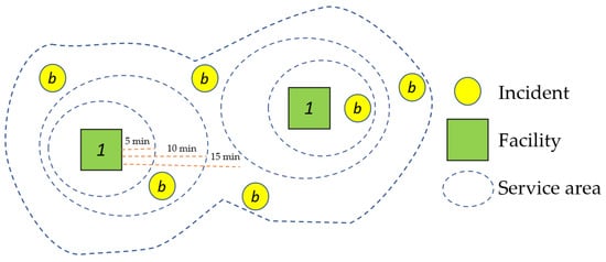
Figure 4.
Illustration of service area analysis.
- Load healthcare locations as the facilities, Y = (, , …… ).
- Set “drive-time” as the impedance and determine the drive-time by 5, 10, and 15 min.
- Ignore invalid locations to avoid errors in the justification process.
- Apply one-way and hierarchical as the restriction.
- Set the direction of transportation using “toward facility”, as the simulation assumes that the time and length are finished at the facility.
- Set the overlay type as “rings” and multiple facility option as “merge by break value” so that each facility will have an area that overlaps with the same neighborhood drive-time.
- In the after-flood scenario, apply impacted bridges as point barriers, impacted roads as line barriers, and inundation areas as polygon barriers.
- Solve.
This research performs Origin-Destination (OD) Cost Matrix analysis to simulate evacuation processes. OD Cost Matrix analysis calculates the cost of transportation for incidents with origin and facilities as destination , and choose which facilities are nearest to each incident. In general, OD Cost matrix analysis consists of four major steps: (1) trip generation, (2) trip distribution, (3) modal split, and (4) traffic assignment. Figure 5 illustrates how OD Cost Matrix analysis was performed in this research. Trip generation defines a selected facility based on drive-time , instead of the length of the road or the range of Euclidian distance. The OD Cost Matrix produces virtual lines that link a couple of OD-pairs from origins to several candidates of destinations and determines the rank among generated routes. In addition, the incidents are chosen based on the highest demands of vulnerable populations as the possible demand .
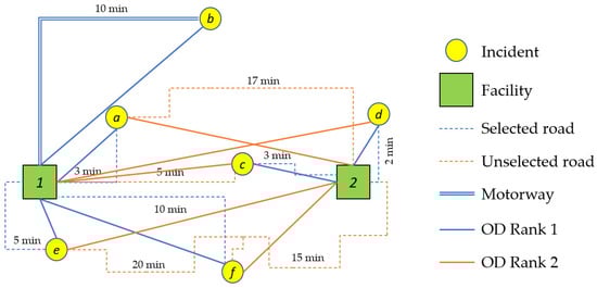
Figure 5.
Illustration of OD Cost Matrix.
In the trip distribution process, the generated sums of trips starting and ending at the centroids are linked to each other to form travel demands (OD-demands, OD-flows, or trip interchanges) for the OD-pairs. It aims to identify by calculating the gravity model as stated from Newton’s Law of gravitation. Equation (7) shows the calculation of travel demand.
where is the origin node, is the destination node weighted with deterrence function
In a modal split process, the measured value is inputted into the utility for drive-time impedance mode . The weighted sum of all , denoted by , together with error value is equal to , with as the corresponding weighted parameter of each measured value [49].
Equation (9) is the multinominal logit model that is used to calculate the probability . This model makes sure the population chooses drive-time mode [50]. After ascertaining the impedance as drive-time, the following process is evaluated with the population as origin using OD-demand = . In this analysis, each link must be the connecting line of one or more travel modes and in the solving procedure, this must be considered. The origins choose among many possible routes to destinations , where is generally infinite according to the number of . Therefore, the solving procedure must follow some assumptions on how the routes are chosen:
- origins will choose a route with the least instantaneous drive-time impedance
- the generated lines, (or synonymously, generalized cost), is the sum of drive-time on the links, including intersections
- each link cost function is assumed to be independent of the flows on all other links or equal to
In the traffic assignment process, the evaluators are referred to as user equilibria. This process yields non-negative route flow variables , , and the link-route incidence variables , , valued to 1 if the link included in route and, 0 otherwise. Equation (10) shows the user equilibria assignment is equal to the optimal solution of the OD cost matrix. Eventually, the route flow or virtual route line is generated based on Equation (13).
3. Results
3.1. Impact Analysis of Flood Inundation
Identification of the impacted area is conducted based on the flood inundation scenario derived from calculation of Landsat 8 spectral indices from the previous study. The flood inundation was delineated to vectors beforehand. Figure 6 presents the highest potential of flood inundation area. Furthermore, the inundation area is overlaid with the infrastructures and healthcare facilities to evaluate the potential of inaccessible infrastructures in amount. The potential inaccessible bridges and roads are represented by red points and red lines, respectively. There are 19 of 169 bridges, 698 road edges, and 2 of 8 healthcare facilities in total that fall within the inundation area.
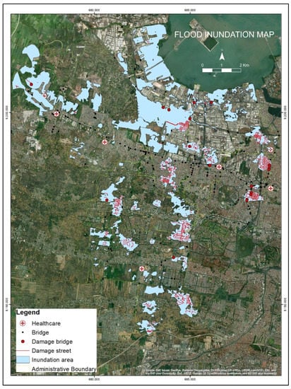
Figure 6.
Area of potential inundation impact.
Table 1 presents the number of inaccessible infrastructures distributed in each district in the West of Surabaya. Sukomanunggal District suffers more than other districts concerning the number of impacted infrastructures. However, the critical location is determined based on how vital the infrastructure is to the neighborhood population when it stops operating [51]. Therefore, this analysis emphasizes the identification of critical infrastructure distribution. It assumes that the allocation of infrastructure concerning road class becomes the crucial factor. Hence, the most critical roads are situated in Asemrowo and Sukomanunggal District accordingly, where it is indicated that the number of motorways and trunk roads are dominant.

Table 1.
The distribution of impacted infrastructure by district.
This result is expected to provide essential information for policymakers to evaluate the function of infrastructure for better enhancement of building resilience. After identifying the number of inaccessible infrastructures, the impacted bridges and roads are involved in the network analysis process as point and line barriers in the after flood scenario.
3.2. Vulnerability Analysis
This research focuses on social vulnerability concerning the exposure of populations. The vulnerability analysis aims to evaluate the degree of vulnerability of populations that may potentially be affected by the flood. Some indicators as mentioned in 2.3 have been calculated and produced various values. Table 2 presents the vulnerability indicator calculation. Regarding the differences in spatial data format, a vectorization is conducted for population data beforehand such that the vectorization process yields a population number per 10,000 m2. Meanwhile, the percentages of gender ratio, children, and elderly remain in vector format, which is distributed in district level. After handling the data format and scale, the calculation of each indicator is conducted. Eventually, V is calculated following Equation (4).
Table 2.
Vulnerability Indicator Calculation.
Figure 7 depicts a univariate map that presents the degree of vulnerability. The vulnerability map is generated with the parcel level as the least spatial scale. Each parcel has a different size of population. To account for the size of populations, the calculation is conducted to classify the index in each district. After normalization, the vulnerability index is divided into 4 classes: slight (0–0.25), moderate (0.25–0.5), high (0.5–0.75), and extreme (0.75–1) in which the degrees are represented by gradation color from green to red, respectively, with the darker color indicating more vulnerability. Table 3 presents the distribution of vulnerability degree and the size of population by district. According to the result, the most vulnerable district is Tandes and Asemrowo District, which is represented by red color. It is caused by the extreme size of populations and high degree of vulnerability in both districts compared to other districts, meaning that the elderly and children population predominantly live closer to the center of Surabaya. Otherwise, the westernmost area has a slight degree of vulnerability. It proves that the distribution of population in Surabaya is also affected by socio-economic attraction to the city center. Furthermore, this output will contribute to the network analysis process.
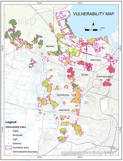
Figure 7.
Vulnerability Map.
Table 3.
The distribution of impacted population by district.
3.3. Network Analysis
3.3.1. Building Network Dataset
A network dataset is a dataset of line or polyline features that are equipped with nodes, junction points, and attributes to solve network problems based on impedance and capacity. The proposed method established a network dataset based on OSM data acquired in 2019. From the export tool of OSM data, this proposed method obtained 8873 road edges and 14,283 junctions and properties relevant to network analysis such as road name, length, one-way, and road class. Hence, a preliminary survey and analysis were conducted to collect the sample of vehicle speeds and drive-times, as well as to complete the one-way attributes. The survey was conducted using a car and handheld Global Positioning System (GPS) on each road class. The survey yielded the speed of each road segment sample. Then, the proposed method calculated the drive-time in the minute unit based on the length and the average speed. In addition, checking the attribute of OSM is also essential before building the network dataset. The export tool of OSM not only exports roads but also other line features such as rivers.
The road network dataset requires roads disjunct in each road edge over the intersections since it represents the route of flow step by step following each road edge. To break road edges, especially roads under the same road names, into multipart edges, a split line at vertices and topology were conducted before establishing the network dataset. This process produces 35,996 road vertices and 31,600 junctions. Figure 8 depicts the differences between before and after the split line at vertices was applied. Figure 8a indicates there are no junctions at each intersection indicated by the red circle. Otherwise, the split line at vertices produces junctions on each road intersection as depicted in Figure 8b. Eventually, the network dataset can be established by setting evaluators as mentioned in 2.5.
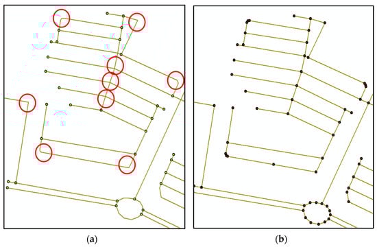
Figure 8.
Differences between (a) before and (b) after split line at vertices applied.
3.3.2. Healthcare Service Area
The healthcare service area generally aims to provide knowledge to the emergency manager about the accessibility of healthcare. The healthcare service area consists of eight hospitals and clinics in the West of Surabaya. Sequentially, this analysis provides a healthcare service area by locating them as candidate shelters. Rather than using length as the impedance, this research uses drive-time to adapt to emergency according to when and where to react more effectively. Besides setting the impedance, one-way restrictions are assigned, and invalid locations are ignored so that the healthcare service area located in the wrong position will be excluded and remain unlocated or erroneously.
The proposed method sets the cut-off time to 5, 10, and 15 min. The parameter setting chooses the route from the incident location to the facilities considering conditions where populations can access the route by themselves or allocated by disaster managers. It means the healthcare facility is only accessible for populations who are situated in the area heading to the facility within these cut-off times. Generally, the service area analysis generates route lines to link facilities to the coverage of incident locations. However, the proposed method only presents the result as a concentric ring to easily distinguish the cut-off time of service areas. The service area analysis is not only proceeded before the flood but also after the flood. Figure 9 presents the output of 5-, 10-, and 15-min service areas before the flood. The areas are represented by darker and lighter colors, respectively. Based on the output result, some 108.31 km2 of 115.23 km2 are located within the healthcare service area. Thereby, 94% of the West of Surabaya is well-serviced and a total of 6.92 m2 are out of service (Table 4). The unserviceable area is presented by the yellow polygon, where most of the area is in Benowo District. It is caused by Benowo District being dominated by a pond rather than settlements. Moreover, Figure 9 depicts the size of impacted populations that overlaid with the healthcare service area. The presented numbers are for each 10,000 m2,, with darker color indicating a larger population. Table 5 presents the size of populations distributed by districts. Hence, the largest size of populations is located in Sukomanunggal district. Furthermore, this output is compared to the service area after the flood.
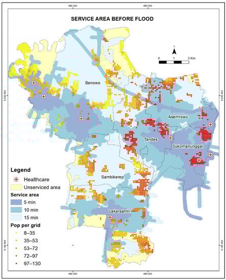
Figure 9.
Healthcare service area before flood.
Table 4.
Comparison of Service area variation.
Table 5.
The size of populations within healthcare service area by district.
Figure 10 depicts the service area after the flooding scenario. There are two healthcare facilities where the surrounding areas are affected by flooding, which causes these facilities to be ignored in the running process and remain as errors. This analysis is conducted assuming the worst impact brought by the flood; thus, the inundation area becomes an additional barrier along with impacted bridges and roads in the analysis. Moreover, the restrictions are not only one-ways and invalid locations but also the inundation area. Consequently, the routes have to avoid the restrictions and find other ways to reach the facilities. Thus, the service area changes significantly and accordingly. Table 4 presents the cumulative changes in the service area of 5-, 10-, and 15-min in all districts. Decremented area occurs in about a half of all areas before flooding for all cut-off times. The most decrement occurs in the 15-min cut-off time area, particularly in Asemrowo and Benowo District. According to the result of impact analysis, Asemrowo District has the most expansive area covered by settlements, and trunk roads predominantly exist to support these behaviors (see Table 1). In summary, barriers play an important role in distinguishing the healthcare coverage area once applied in the flood scenario. Table 5 describes the size of populations with respect to the variation of healthcare service area.
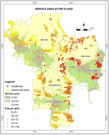
Figure 10.
Healthcare service area after flood.
3.3.3. Route Analysis
This research focuses on handling the emergency response of vulnerable populations. This analysis is conducted to determine which healthcare facility should be accessed between before and after the flood. The parameters used in this analysis are drive-time, one-way restriction, invalid location, and U-turn prohibition. This analysis assigns healthcare facility as the located destination and takes 20 sample points of the high and extreme vulnerable populations in the settlement area as the origins. The analysis makes sure the location of origins is within the service area to minimize the invalid location of origins and ascertain the origins can access routes to healthcare facilities. Figure 11 depicts the output of route analysis in normal conditions, meaning that any barriers are ignored.
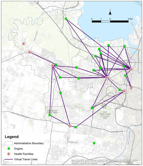
Figure 11.
Route analysis before flood.
This analysis provides the fastest route where the drive-time is the least cost. As applied to a normal condition with no barriers and no invalid locations existing either at the sample points or healthcare facilities, the analysis generates 38 routes according to the OD Cost Matrix analysis. Each origin is allocated to choose two healthcare service facilities among eight candidates based on the optimal solution and the two options are ranked. This analysis generates a virtual travel line based on the actual measured drive time. The output route is presented by purple lines, while the sample points are presented by green dots.
Table 6 presents the drive-time of each output route. The fastest route takes 1.883 min from origin location 3 to destination location 8. Meanwhile, the latest route takes 19.209 min from origin location 8 to destination location 8. According to the impacted population, location 5 accounted for the greatest size of the impacted population. However, the capacity of healthcare could not fulfill the demands. In other words, the reevaluation of candidate shelters must be carried out. Moreover, route analysis is conducted to generate routes in flood conditions. It aims at knowing how effective the network analysis is to solve the routing problem even applied to an emergency.
Table 6.
Evacuation route time, population (Pop), and healthcare capacity before flood.
In comparison, this analysis simulates the worst effect scenario for the transportation network brought about by the flood. The worst effects refer to the severity of casualties, inaccessible transportation areas due to the inundation, road blockages, and damaged roads. Figure 12 depicts the output routes from the OD Cost Matrix analysis after the flood scenario. The parameters of analysis are the same as before the flood. Additionally, this analysis uses the same scenario as service area analysis for after the flood; thus, two healthcare facilities remain as invalid locations. Consequently, the result generates 30 routes that are presented by the magenta line with a maximum travel time of 32.127 min and the minimum travel time of 1.883 min. In the after-flood scenario, the origins tend to choose another candidate destination as it is affected by avoiding the point and line barriers. Although most healthcare facilities are situated in the city center, the critical roads are also located in the city center, which causes accessibility to face a massive barrier when an emergency occurs such as a flood, road blockage, damaged bridge, and damaged road. Table 7 presents the population, evacuation time, and the change in travel to the destination. In addition to investigating the travel time comparing both before and after the flood scenario, Table 8 summarizes the travel time gap. Overall, the greatest time gap is −10.446 min for travel from origin location 4 to destination location 2.
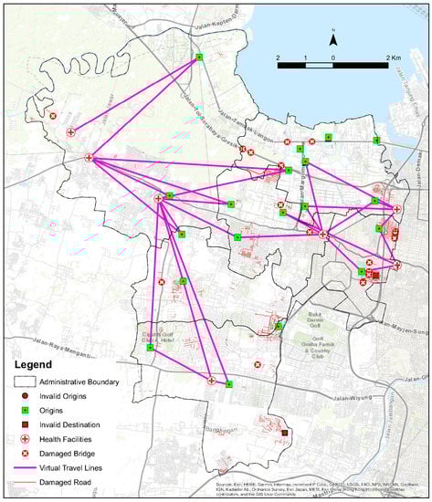
Figure 12.
Route analysis after flood.
Table 7.
Evacuation route time, population (Pop), and healthcare capacity after flood.
Table 8.
Comparison of travel time for the same origins and destinations.
4. Discussion
Since a disaster cannot be predicted, understanding the condition of vulnerability is quite important to properly minimize the impact of the disaster. Vulnerability refers to the propensity of populations, communities, infrastructures, environments to suffer when a hazard occurs [45,52]. Vulnerability is a multidimensional context that combines physical, economic, mental, social, and environmental factors as evaluators to assess the probability of survival [53]. By understanding the degree of vulnerability, the emergency manager can effectively prioritize the location where the high probability of the vulnerable population is located. Vulnerable populations refer to the populations in need of evacuation assistance, such as the elderly, children, low-income groups, and the physically and mentally disabled [54], as the evacuation is a major activity to reduce exposure [52].
The effectiveness of evacuation not only depends on the location of impacted populations, but also accessibility, availability of shelters, evacuation zones, transportation routes, and evacuation time [55,56]. Even time is life in emergency responses, meaning that any delayed actions may result in unnecessary casualties and suffering populations [57]. Therefore, minimizing the response time becomes the ultimate goal in dealing with critical time. Many studies have been conducted to optimize response time. For example, ref. [21] optimizes the dispatching and routing of emergency vehicles in disaster situations by understanding patient priorities, clustering the criteria, and minimizing the distance, as well as understanding congestion on road links. Since the preliminary information about demands is gathered beforehand, the response time can be minimized. Therefore, accessibility indeed plays a key role in emergency response [58,59]. Accessibility in emergency response has strong links to the transportation network and healthcare facilities in terms of what effects might happen to transportation when an emergency occurs and how healthcare facilities serve the populations considering the capacity, availability, acceptability, and affordability [15,17,25,59]. Therefore, possessing preliminary knowledge must be an emerging solution for supporting emergency managers under time-sensitive conditions.
There are three major aspects of accessibility that must be covered. It consists of spatial distribution and healthcare characteristics, a transportation system that links the population to healthcare facilities, and socio-economic characteristics of individuals that will access the healthcare facilities [17]. As road networks are the basic data for accessibility analysis [26], this research focuses on the optimization of the transportation system in emergency management. By leveraging and enriching the road network with related information, this research expects to generate better service area and route analysis. The road networks must be generated by accounting for real-world road networks with existing damaged roads and congestion [21]. Instead of using a modeling approach to enrich the speed attributes, a preliminary survey was conducted to collect the average speed. It aims to experience the real conditions on the road and eventually generate drive-times, which become one of the parameters to build a network dataset.
By simulating flood scenarios (before and after), this research generates the most vulnerable populations and healthcare service areas. Healthcare accessibility is assessed to be an important factor in disaster risk management, as it provides emergency care to the injured, trauma care, and surgery [16]. Thus, the accessibility faces a time-sensitive emergency. Therefore, this research uses drive-time instead of length as the cost in the network analysis. Consequently, the results are generated based on the fastest instead of the shortest routes. Healthcare accessibility is depicted by service areas within a variety of drive-times. The variations of the service area are also overlaid with the vulnerable populations, who are regarded as healthcare demand sources. The results indicate that the healthcare service area covers almost the whole of West Surabaya under normal situations. Nevertheless, once the worst scenario is applied, the service area decreases significantly, especially where the critical infrastructure is located in the after-flood scenario. By assigning barriers in the after scenario, the network analysis successfully generates the safest routes with minimum different drive-time from before.
This research provides knowledge about the vulnerable district and the variations of healthcare accessibility in the spatial perspective. It is expected to be a contribution to disaster management in Surabaya. By understanding the distribution of vulnerable populations, the policymaker knows where and who to be prioritized. Moreover, by considering the worst situation that has been simulated in this research, the policymaker can know if an area is out of service. For future study, this research recommends evaluating possible shelter locations apart from healthcare centers to compensate for areas that are out of service. Furthermore, additional indicators are required to be considered in future work in terms of determining the location of appropriated shelters i.e., historical disaster record, slope, land use, and healthcare treatment type.
5. Conclusions
Using GIS to support evacuation planning in terms of providing vulnerability analysis and healthcare accessibility was successfully implemented. The vulnerability analysis generates the degree of vulnerability of populations, consisting of slight, moderate, high, and extreme. The vulnerability is determined based on the size of population, gender ratio, elderly, and children exposed to the potential of flood inundation. The results show that the most vulnerable population live in Asemrowo and Tandes Districts, which are closest to the center of Surabaya. Since almost the whole of West Surabaya is covered by healthcare service areas, the vulnerable population can be well-serviced accordingly. Unless the flood-affected infrastructure is damaged or inaccessible, the healthcare service area and route analysis of the before and after flood scenario can produce the optimum network solutions. The results prove that the use of network analysis capable of optimizing time-cost and safety.
Author Contributions
Conceptualization, Nurwatik Nurwatik and Jung-Hong Hong; methodology, Nurwatik Nurwatik; software, Hepi Hapsari Handayani; formal analysis, Nurwatik Nurwatik; resources, Hepi Hapsari Handayani; data curation, Mohammad Rohmaneo Darminto; writing—original draft preparation, Nurwatik Nurwatik; writing—review and editing, Nurwatik Nurwatik; visualization, Nurwatik Nurwatik; supervision, Nurwatik Nurwatik; project administration, Agung Budi Cahyono; funding acquisition, Lalu Muhamad Jaelani. All authors have read and agreed to the published version of the manuscript.
Funding
This research was funded by the Directorate of Research and Community Service (DRPM-ITS), Institut Teknologi Sepuluh Nopember, grant number 1212/PKS/ITS/2019.
Institutional Review Board Statement
Not applicable.
Informed Consent Statement
Not applicable.
Data Availability Statement
The data presented in this study are openly available in www.worldpop.org (21 January 2020), https://tanahair.indonesia.go.id/portal-web (22 February 2019), and https://export.hotosm.org/ (24 January 2019).
Acknowledgments
The author acknowledges with deep thanks DRPM-ITS for technical and financial support. The author also acknowledges the great support of the Department of Geomatics Engineering.
Conflicts of Interest
The authors declare no conflict of interest.
References
- Gunes, A.E.; Kovel, J.P. Using GIS in Emergency Management Operations. J. Urban Plan. Dev. 2001, 126, 136–149. [Google Scholar] [CrossRef]
- Pacific Humanitarian Team. Emergency Preparedness & Response Plan A Guide to Inter-Agency Humanitarian Action in the Pacific, 1st ed.; OCHA Regional Office for the Pasific: Suva, Fiji, 2013; pp. 1–84. [Google Scholar]
- Mansourian, A.; Rajabifard, A.; Valadan Zoej, M.J.; Williamson, I. Using SDI and web-based system to facilitate disaster management. Comput. Geosci. 2006, 32, 303–315. [Google Scholar] [CrossRef]
- Huder, R.C. Disaster Operations and Decision Making; JOHN WILEY & SONS, Inc.: Hoboken, NJ, USA, 2012; ISBN 9780309123983. [Google Scholar]
- BMKG. Prakiraan Musim Kemarau 2019 di Indonesia; Badan Meteorologi Klimatologi dan Geofisika: Jakarta, Indonesia, 2019; pp. 1–141.
- Saydi, M.; Zoej, V.M.J.; Mansourian, A. Design and implementation of a Web-based GIS (in response phase) for earthquake disaster management in Tehran City. ISPRS High Resolut. Earth Imaging Geospat. Inf. Workshop 2004, 35, 678–681. [Google Scholar]
- Van Westen, C. Remote Sensing and GIS for Natural Hazards Assessment and Disaster Risk Management. Treatise Geomorphol. 2013, 3, 259–298. [Google Scholar] [CrossRef]
- Taramelli, A.; Melelli, L.; Pasqui, M.; Sorichetta, A. Estimating hurricane hazards using a GIS system. Nat. Hazards Earth Syst. Sci. 2008, 8, 839–854. [Google Scholar] [CrossRef]
- Tang, A.; Ran, C.; Wang, L.; Gai, L.; Dai, M. Intelligent Digital System in Urban Natural Hazard Mitigation. In Proceedings of the 2009 WRI World Congress on Software Engineering, Xiamen, China, 9–21 May 2009; pp. 355–359. [Google Scholar] [CrossRef]
- Nichols, E.N.; Bradley, D.L.; Zhang, X.; Faruque, F.S.; Duhe, R.J. The geographic distribution of mammography resources in Mississippi. Online J. Public Health Inform. 2014, 5, 1–20. [Google Scholar] [CrossRef] [Green Version]
- Alparslan, E.; Ince, F.; Erkan, B.; Aydöner, C.; Özen, H.; Dönertaş, A.; Ergintav, S.; Yaǧsan, F.S.; Zateroǧullari, A.; Eroǧlu, I.; et al. A GIS model for settlement suitability regarding disaster mitigation, a case study in Bolu Turkey. Eng. Geol. 2008, 96, 126–140. [Google Scholar] [CrossRef]
- ESRI. GIS and Emergency Management in Indian Ocean Earthquake/Tsunami Disaster; Environmental Systems Research Institute: New York, NY, USA, 2006; pp. 1–40. [Google Scholar]
- Ai, F.; Comfort, L.K.; Dong, Y.; Znati, T. A dynamic decision support system based on geographical information and mobile social networks: A model for tsunami risk mitigation in Padang, Indonesia. Saf. Sci. 2016, 90, 62–74. [Google Scholar] [CrossRef]
- Miraliakbari, A.; Hahn, M.; Maas, H.G. Development of a multi-sensor system for road condition mapping. Int. Arch. Photogramm. Remote Sens. Spat. Inf. Sci. ISPRS Arch. 2014, 40, 265–272. [Google Scholar] [CrossRef]
- Levinson, D.R. Hospital Emergency Preparedness and Response during Superstorm Sandy; American Hospital Association: Washinton, DC, USA, 2014; pp. 1–39. [Google Scholar]
- World Health Organization United Kingdom Health Protection Agency and Partners Disaster Risk Management for Health SAFE HOSPITALS. PREPARED FOR EMERGENCIES AND DISASTERS. Disaster Risk Management Health Fact Sheet; United Kingdom. 2011, pp. 1–2. Available online: https://www.who.int/hac/events/drm_fact_sheet_safe_hospitals.pdf?ua=1 (accessed on 1 March 2022).
- Murad, A. Using GIS for determining variations in health access in jeddah city, Saudi Arabia. ISPRS Int. J. Geo-Inf. 2018, 7, 254. [Google Scholar] [CrossRef] [Green Version]
- Gingerich, B.S. A Performance Review of FEMA’s Disaster Management Activities in Response to Hurricane Katrina. Home Health Care Manag. 2006, 20, 352–353. [Google Scholar] [CrossRef]
- George, D.; Haddow, J.A.B.; Coppola, D.P. Introduction to Emergency Management Fourth Edition; Elsevier: Burlington, VT, USA, 2011; pp. 1–423. [Google Scholar]
- Chu, H.J.; Lin, B.C.; Yu, M.R.; Chan, T.C. Minimizing spatial variability of healthcare spatial accessibility—the case of a dengue fever outbreak. Int. J. Environ. Res. Public Health 2016, 13, 1235. [Google Scholar] [CrossRef]
- Jotshi, A.; Gong, Q.; Batta, R. Dispatching and routing of emergency vehicles in disaster mitigation using data fusion. Socioecon. Plann. Sci. 2009, 43, 1–24. [Google Scholar] [CrossRef]
- Dong, S.; Wang, H.; Mostafavi, A.; Gao, J. Robust component: A robustness measure that incorporates access to critical facilities under disruptions. J. R. Soc. Interface 2019, 16, 1–15. [Google Scholar] [CrossRef] [PubMed] [Green Version]
- Dong, S.; Esmalian, A.; Farahmand, H.; Mostafavi, A. An integrated physical-social analysis of disrupted access to critical facilities and community service-loss tolerance in urban flooding. Comput. Environ. Urban Syst. 2020, 80, 101443. [Google Scholar] [CrossRef]
- Alamdar, F.; Kalantari, M.; Rajabifard, A. Towards multi-agency sensor information integration for disaster management. Comput. Environ. Urban Syst. 2016, 56, 68–85. [Google Scholar] [CrossRef]
- Rekha, R.S.; Wajid, S.; Radhakrishnan, N.; Mathew, S. Accessibility Analysis of Health care facility using Geospatial Techniques. Transp. Res. Procedia 2017, 27, 1163–1170. [Google Scholar] [CrossRef]
- Guth, J.; Wursthorn, S.; Keller, S. Multi-parameter estimation of average speed in road networks using fuzzy control. ISPRS Int. J. Geo-Inf. 2020, 9, 55. [Google Scholar] [CrossRef] [Green Version]
- Winn, M.T. A Road Network Shortest Path AnalysisL Applying Time-Varying Travel-Time Costs for Emergency Response Vehicle Routing. Master’s Thesis, Northwest Missouri State University, Marryville, MO, USA, January 2014. [Google Scholar]
- Bhanumurthy, V.; Bothale, V.M.; Kumar, B.; Urkude, N.; Shukla, R. Route Analysis for Decesion Support System in Emergency Management Through Gis Technologies. Int. J. Adv. Eng. Glob. Technol. 2015, 3, 345–350. [Google Scholar]
- Nicoara, P.-S.; Haidu, I. A Gis Based Network Analysis for the Identification of Shortest Route Access To Emergency Medical Facilities. Geogr. Tech. 2014, 09, 60–67. [Google Scholar]
- Girres, J.; Touya, G. Quality Assessment of the French OpenStreetMap dataset. Trans. GIS 2019, 14, 435–459. [Google Scholar] [CrossRef]
- Jackson, S.P.; Mullen, W.; Agouris, P.; Crooks, A.; Croitoru, A.; Stefanidis, A. Assessing completeness and spatial error of features in volunteered geographic information. ISPRS Int. J. Geo-Inf. 2013, 2, 507–530. [Google Scholar] [CrossRef]
- UNFPA; BNPB; BPS. Guidelines for the Use of Population Data in Disaster; United Nations Population Fund: Jakata, Indonesia, 2014; pp. 1–95.
- Chu, J. A statistical analysis of the novel coronavirus (COVID-19) in Italy and Spain. PLoS ONE 2021, 16, e0249037. [Google Scholar] [CrossRef]
- Zhao, L.; Li, H.; Sun, Y.; Huang, R.; Hu, Q.; Wang, J.; Gao, F. Planning emergency shelters for urban disaster resilience: An integrated location-allocation modeling approach. Sustainability 2017, 9, 2098. [Google Scholar] [CrossRef] [Green Version]
- Chen, W.; Fang, Y.; Zhai, Q.; Wang, W.; Zhang, Y. Assessing emergency shelter demand using POI data and evacuation simulation. ISPRS Int. J. Geo-Inf. 2020, 9, 41. [Google Scholar] [CrossRef] [Green Version]
- Yao, Y.; Zhang, Y.; Yao, T.; Wong, K.; Tsou, J.Y.; Zhang, Y. A GIS-based system for spatial-temporal availability evaluation of the open spaces used as emergency shelters: The case of Victoria, British Columbia, Canada. ISPRS Int. J. Geo-Inf. 2021, 10, 63. [Google Scholar] [CrossRef]
- BPS Rata-Rata Tinggi Wilayah di Atas Permukaan Air Laut (DPL) Menurut Pos Hujan di Kabupaten/Kota di Provinsi Jawa Timur. Available online: https://jatim.bps.go.id/linkTabelStatis/view/id/105 (accessed on 24 February 2022).
- Watik, N.; Jaelani, L.M. Flood evacuation routes mapping based on derived-flood impact analysis from landsat 8 imagery using network analyst method. Int. Arch. Photogramm. Remote Sens. Spat. Inf. Sci. ISPRS Arch. 2019, 42, 455–460. [Google Scholar] [CrossRef] [Green Version]
- University of Southampton Open Spatial Demographic Data and Research. Available online: https://www.worldpop.org/ (accessed on 21 January 2020).
- Stevens, F.R.; Gaughan, A.E.; Linard, C.; Tatem, A.J. Disaggregating census data for population mapping using Random forests with remotely-sensed and ancillary data. PLoS ONE 2015, 10, e0107042. [Google Scholar] [CrossRef] [Green Version]
- BIG Indonesia Geospatial Portal. Available online: https://tanahair.indonesia.go.id/portal-web (accessed on 22 February 2019).
- Xu, H. Modification of Normalized Difference Water Index (NDWI) to Enhance Open Water Features in Remotely Sensed Imagery. Int. J. Remote Sens. 2007, 27, 3025–3033. [Google Scholar] [CrossRef]
- Rasul, A.; Balzter, H.; Faqe, G.R.; Id, I.; Hameed, H.M. Applying Built-Up and Bare-Soil Indices from Landsat 8 to Cities in Dry Climates. Land 2018, 7, 81. [Google Scholar] [CrossRef] [Green Version]
- Rovins, J.E.; Wilson, T.M.; Hayes, J.; Jensen, S.J.; Dohaney, J.; Mitchell, J.; Johnston, D.M.; Davies, A. Risk Assessment Handbook. 2015. ISBN 9780908349357. Available online: https://www.researchgate.net/publication/290883771_Risk_Assessment_Handbook (accessed on 1 March 2022).
- Cardona, O.; Van Aalst, M.K.; Birkmann, J.; Fordham, M.; Mc Gregor, G.; Rosa, P.; Pulwarty, R.S.; Schipper, E.L.F.; Sinh, B.T.; Décamps, H. Determinants of Risk: Exposure and Vulnerability. In Managing the Risks of Extreme Events and Disasters to Advance Climate Change Adaptation: Special Report of the Intergovernmental Panel on Climate Change; Cambridge University Press: Cambridge, UK, 2012; pp. 65–108. [Google Scholar] [CrossRef] [Green Version]
- BNPB. Indeks Resiko Bencana Indonesia; Direktorat Pengurangan Risiko Bencana Badan National Penanggulangan Bencana: Jakarta, Indonesia, 2018; pp. 1–328.
- Sari, F.; Erdi, A. A Network Analyst Design for Providing the Shortest Intervention Time of the Emergency Vehicles as Like Ambulance and Fire Fighting to the Emergency Events, a Case Study Konya. In Proceedings of the FIG Working Week, Roma, Italy, 6–10 May 2012. [Google Scholar]
- Wang, S.X. The improved Dijkstra’s shortest path algorithm and its application. Procedia Eng. 2012, 29, 1186–1190. [Google Scholar] [CrossRef] [Green Version]
- Peterson, A. The Origin-Destination Matrix Estimation Problem: Analysis and Computations. Ph.D. Thesis, Department of Science and Technology, Linköpings Universitet, Norrköping, Sweden, May 2007. [Google Scholar]
- Wang, Y.; Ma, X.; Liu, Y.; Gong, K.; Henricakson, K.C.; Xu, M.; Wang, Y. A two-stage algorithm for origin-destination matrices estimation considering dynamic dispersion parameter for route choice. PLoS ONE 2016, 11, e0149827. [Google Scholar] [CrossRef] [PubMed] [Green Version]
- Ranke, U. Natural Disaster Risk Management; Springer International Publishing: Berlin/Heidelberg, Germany, 2016; ISBN 978-3-642-11473-1. [Google Scholar]
- Russo, F.; Rindone, C.; Trecozzi, M.R. The role of training in evacuation. WIT Trans. Inf. Commun. Technol. 2012, 44, 491–502. [Google Scholar] [CrossRef] [Green Version]
- Tascón-González, L.; Ferrer-Julià, M.; Ruiz, M. Eduardo García-Meléndez Social Vulnerability Assessment for Flood. Water 2020, 12, 558. [Google Scholar] [CrossRef] [Green Version]
- Li, M.; Xu, J.; Liu, X.; Sun, C.; Duan, Z. Use of shared-mobility services to accomplish emergency evacuation in urban areas via reduction in intermediate trips-Case study in Xi’an, China. Sustainability 2018, 10, 4862. [Google Scholar] [CrossRef] [Green Version]
- Carley, K.M.; Malik, M.; Landwehr, P.M.; Pfeffer, J.; Kowalchuck, M. Crowd sourcing disaster management: The complex nature of Twitter usage in Padang Indonesia. Saf. Sci. 2016, 90, 48–61. [Google Scholar] [CrossRef] [Green Version]
- Kwan, M.P.; Lee, J. Emergency response after 9/11: The potential of real-time 3D GIS for quick emergency response in micro-spatial environments. Comput. Environ. Urban Syst. 2005, 29, 93–113. [Google Scholar] [CrossRef]
- Jiang, Y.; Yuan, Y. Emergency logistics in a large-scale disaster context: Achievements and challenges. Int. J. Environ. Res. Public Health 2019, 16, 779. [Google Scholar] [CrossRef] [PubMed] [Green Version]
- Burdziej, J. A Web-based spatial decision support system for accessibility analysis- concepts and methods. Appl Geomat 2012, 4, 75–84. [Google Scholar] [CrossRef] [Green Version]
- Leiser, C.L.; Anderson, R.E.; Martin, C.; Hanson, H.A.; O’Neil, B. Combining Drive Time and Urologist Density to Understand Access to Urologic Care. Urology 2020, 139, 78–83. [Google Scholar] [CrossRef] [PubMed]
Publisher’s Note: MDPI stays neutral with regard to jurisdictional claims in published maps and institutional affiliations. |
© 2022 by the authors. Licensee MDPI, Basel, Switzerland. This article is an open access article distributed under the terms and conditions of the Creative Commons Attribution (CC BY) license (https://creativecommons.org/licenses/by/4.0/).