A Vector Data Model for Efficiently Rendering Large Vector Maps on Global 3D Terrain Surfaces

Abstract

Visualizing vector data on 3D terrain surfaces is a basic and essential function in 3D GIS. However, due to the complexity of vector data structures, efficient and effective organization of the vector data is a key issue for the efficient display of vector data in 3D. In this paper, we present a new Vector Tiled Pyramid Model to organize and manage vector data so that they can be visualized on 3D terrain surfaces more effectively. In the Vector Tiled Pyramid Model, vector data at different scales within the same geographical extent are stored as separate levels. Each vector level in our proposed model is divided into vector tiles of fixed sizes organized in a grid index. This improves the efficiency of visualizing vector data on 3D terrain surfaces. Preliminary experimental results suggest that the proposed Vector tiled Pyramid Model, compared with the traditional vector database scheme, can help us to visualize vector data on 3D terrain surfaces more efficiently. In addition, this advantage is more evident when a vector tile at a lower level (large-scale) is requested and visualized on 3D terrain surfaces.

1. Introduction

With the development of 3D GIS, massive vector data need to be displayed in 3D scenes [1,2]. A suitable vector data organization scheme is critical to improving the efficiency of data access, thereby enhancing the efficiency of expression vector data, especially when visualizing large vector maps on 3D terrain surfaces.

Currently, there are two main schemes for organizing and visualizing vector data on 3D terrain surfaces. The first scheme is the traditional vector database. In this scheme, vector data are stored in GIS databases but with data structures that are often vendor-specific, such as ArcSDE by ESRI, Inc. or Oracle Spatial by Oracle. Generally, multi-resolution techniques are adopted when displaying vector data in 3D. The original vector data are simplified to form a multi-resolution vector map [3,4,5] with spatial indexes [6]. This data organization scheme stores vector data in a database in the form of coordinates and their topological relationships and can be combined with a variety of rendering methods (texture-based methods and geometry-based methods) to visualize vector data. This data organization scheme accesses vector data objects from the database in real-time when the displayed vector objects are queried. Thus, it is inefficient when processing large volumes of vector data.

The second data organization scheme is the texture tiled pyramid as discussed by Kersting et al [7]. In a texture tiled pyramid, vector data are first rasterized to raster levels at different resolutions. Each raster level is partitioned into many blocks, which can also be called texture tiles. When rendering the data, based on the tile-map technique, texture tiles are used for efficient and high-quality image visualizations. This scheme is efficient for rendering vector data and used for visualizing large volumes of vector data over large geographic extents, such as the Web Map Tile Service of Open GIS Consortium. However, this data organization scheme adopts the form of raster data to organize the vector data, which will lose the specific details found in vector data during the process of rasterization [8].

In this paper, we propose a new Vector Tiled Pyramid Model to organize and manage vector data at a global scale that enhances rendering efficiency when visualizing vector data in 3D. Similar to the texture tiled pyramid, the different levels in the Vector Tiled Pyramid Model are different scales. Each vector data level is partitioned into many blocks. These blocks are also called vector tiles and are stored as a grid index. Together, they form a hierarchical data model for storing vector data with different details.

The Vector Tiled Pyramid Model accelerates access to vector data by bypassing irrelevant data entities at each data level. This is achieved by locating the vector tile that contains the location of interest so that none of the other vector tiles need to be processed or searched. The block structure of our proposed model makes it possible to access a data entity by only processing those vector tiles containing the entities of interest found at different levels to the same extent.

The layout of this article is as follows: Section 2 introduces the tiled pyramids and the associated methods for rendering vector data on 3D terrain. Section 3 and Section 4 describe the definition of the Vector Tiled Pyramid Model and how to organize the vector data using the Vector Tiled Pyramid Model. Section 5 introduces a series of experiments and analyses of their results. Finally, Section 6 draws a conclusion about this paper.

2. Related Work

2.1. Tiled Pyramids

Image Pyramids are a hierarchy of fine to coarse resolution versions of an image [9,10]. It is an important concept for image filtering and analysis at multiple scales. Using a compression scheme for images, a multi-level structure based on the original image is constructed in an Image Pyramid [11]. The bottom level of an Image Pyramid is comprised of the original images [12]. From the bottom level to the top level of an Image Pyramid, the resolution levels are smaller and smaller. Image Pyramids are a space for time strategy, which can speed up image processing operations.

With the development of remote sensing technology, there has been a huge increase in the resolution of image data. This creates some data processing problems in the transmission and visualization of images. Tiled Pyramids [13,14], are variations of Image Pyramids and an effective strategy to deal with these issues. Terrain data [15,16] and satellite images [17,18], when coded like images, can be built into a hierarchical multi-resolution representation as Tiled Pyramids. Tiled Pyramids are a kind of multi-resolution hierarchical model, whose structure flows from the bottom level to the top level of the Tiled Pyramid at a lower and lower resolution for the same geographic area [19,20].

As an application of the Tiled Pyramids, map tile technology [21], which produces a number of square pictures cut by the map with coordinates according to a fixed set of scales (tile level) and specified image size, has been widely used in the application based on maps, such as OpenStreetMap, Google Maps [22]. Map tiles are a set of pre-generated map images based on geographic vector data, such as the Web Map Tile Service of the Open GIS Consortium [23].

2.2. The Methods for Rendering Vector Data on 3D Terrain

At present, there are two kinds of methods used to render vector data on 3D terrain surfaces: the geometry-based and texture-based methods. Geometry-based methods [24,25], using elevation interpolation, process vector data to obtain 3D coordinates. Using 3D rendering techniques such as OpenGL, vector data are visualized on 3D terrain surfaces. The visualization resulting from the geometry-based methods is often detailed and aesthetically pleasing. For example, the geometry-based methods were adopted in Google Earth, a virtual globe, map, and geographical information program, to render the boundary line vector data.

In texture-based methods [26,27], vector data are rasterized into texture data and mapped to a 3D terrain surface using texture mapping technology. This is a highly efficient method for expression vector data. For example, in some large vector map processing applications, texture-based methods are often used to visualize the polygon vector data. Although currently, geometry-based methods can achieve 3D visualization of the polygon vector data, using triangulation [28,29] or the stencil shadow volume algorithm [8], these are inefficient and cannot meet the needs of large scene rendering the 3D scene.

Taking into account the characteristics of the two different schemes, based on our proposed Vector Tiled Pyramid Model, the geometry-based and texture-based methods are adopted in this paper, respectively, handling different types of vector data.

In addition to the above two rendering schemes, data simplification also facilitates rendering. In vector data simplification, a subset of the original vector data is produced from the original vector data under a set tolerance. The Douglas-Peucker algorithm [30] is a classic line simplification algorithm that maintains the geometric characteristics of the original data [31]; however, it may produce inconsistent topological relations. For example, it is possible that two disjointed lines intersect after simplification with the Douglas-Peucker algorithm.

3. The Vector Tiled Pyramid Model

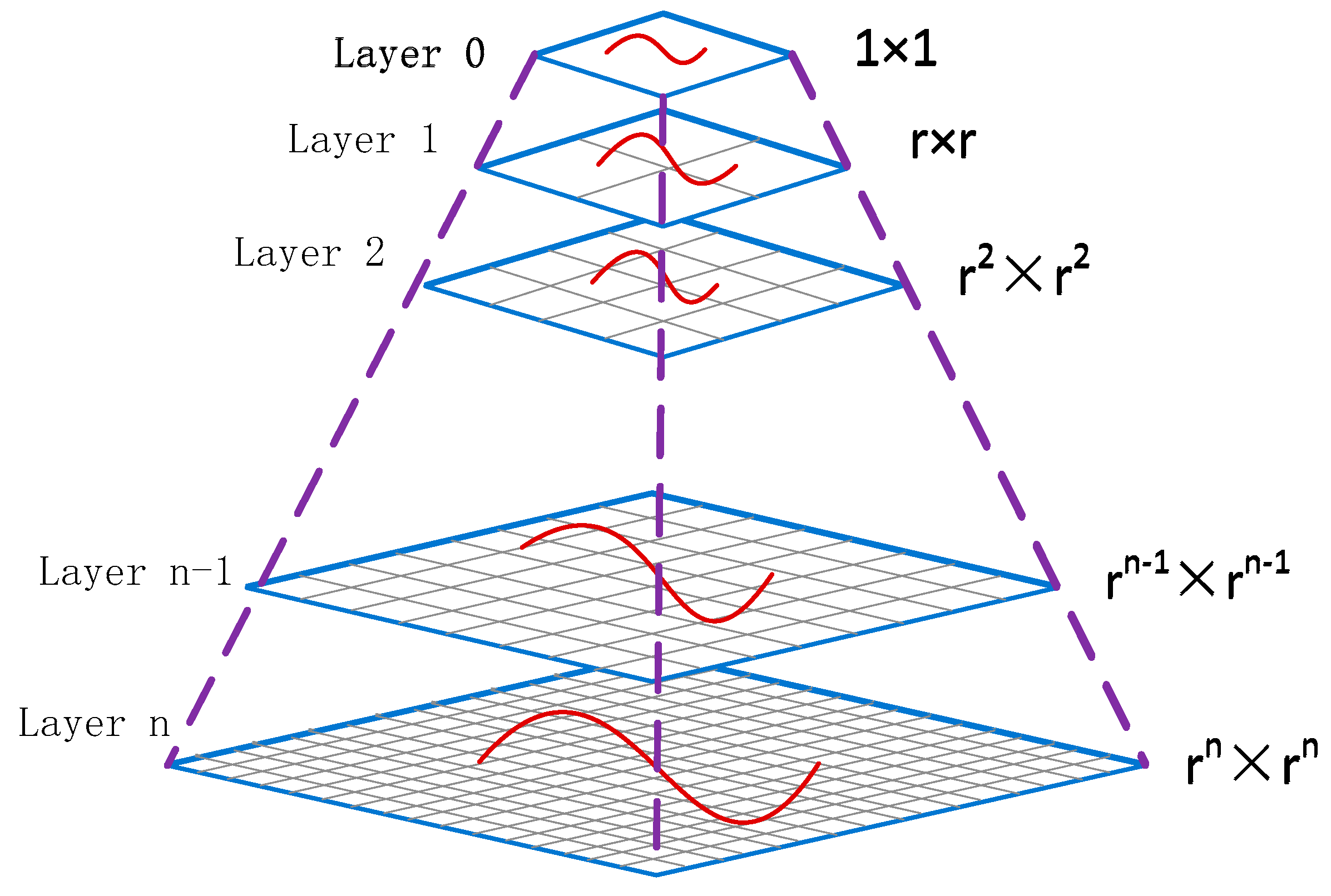
Our proposed Vector Tiled Pyramid Model (VTPM) is a data model that organizes and manages vector data. As seen in Figure 1, it consists of a sequence of vector data levels that are copies of original data but at decreasing levels of geographic detail from the bottom level to the top level of the model. Zoom levels are stratified, each level represents a corresponding map scale. In Figure 1, vector data at the same level is partitioned into several data blocks at a fixed size. Each data block in the VTPM is considered a vector tile.

For a vector tile, an effective mechanism for spatial indexing needs to be established. Because the division of a vector tile follows a fixed rule, we use the row number and column number of the vector tile in the model to code the vector tiles. Each vector tile is coded using the level, row, and column number. Level numbers increase from top to bottom, starting with zero. Row numbers increase from up and down, starting with zero. Column numbers increase from left to right, also starting at zero. By coding the vector tiles, we can use their index numbers to compute and identify the spatial range of any vector tile, which in turn supports efficient spatial queries

The VTPM stores vector data at different levels with different details. As shown in Figure 1, in the VTPM, the top level of the model, which has only one vector tile, is defined as level zero. The level number of each level in the VTPM sequentially increases until the bottom level of the VTPM. There are more and more detailed vector data at each increasing level, forming a collection of multi-scale vector data. The following four definitions provide the parameters for our VTPM:

Definition 1.

The spatial range of the VTPM (S) is the spatial extent corresponding to the vector tiles of each level.

Generally, the spatial range of the VTPM depends on the spatial extent of the original vector data. For example, if we want to deal with global vector data, we can use the global geographic scope as the spatial range of the VTPM. If we want to deal with the vector data of a country or a city, we take the spatial range of the country or a city as the spatial range for the VTPM.

Definition 2.

The number of levels of the VTPM (N) refers to the number of replications based on the original data.

The number of levels of the VTPM depends on how many different levels of the data we want to show when the vector tile is displayed on the 3D terrain.

Definition 3.

The ratio between the vector tiles at adjacent levels (R) refers to the proportional relationship in the geographical scope of the vector tiles between adjacent levels.

As shown in Figure 1, a vector tile at the higher level was divided into r*r equal parts at the lower level; meanwhile, the geographic scope of the vector tile at the higher level is equal to the geographic scope of the r*r vector tiles at the lower level. In contrast to the vector tile at the higher level, there is more detailed vector data at the vector tiles at the lower level.

Definition 4.

The simplification threshold of the VTPM (T) refers to the compression threshold in vector data simplification when the vector tiles of different levels are produced based on the original vector data.

The simplification threshold of the VTPM is a crucial parameter for the VTPM. It determines how many details the vector data contains at each level of the VTPM. Generally speaking, from the top level to the bottom level of the VTPM, the simplification threshold for vector data simplification corresponding to the same level of the VTPM becomes smaller and smaller. This ensures that the level of detail varies continuously at different levels of the VTPM, thereby forming a pyramid structure. The choice of the simplification threshold is determined by a specific VTPM application. In the experimental part of this paper, we propose a method to determine the simplification threshold at different levels in the VTPM. This will be elaborated on in Section 4.1.

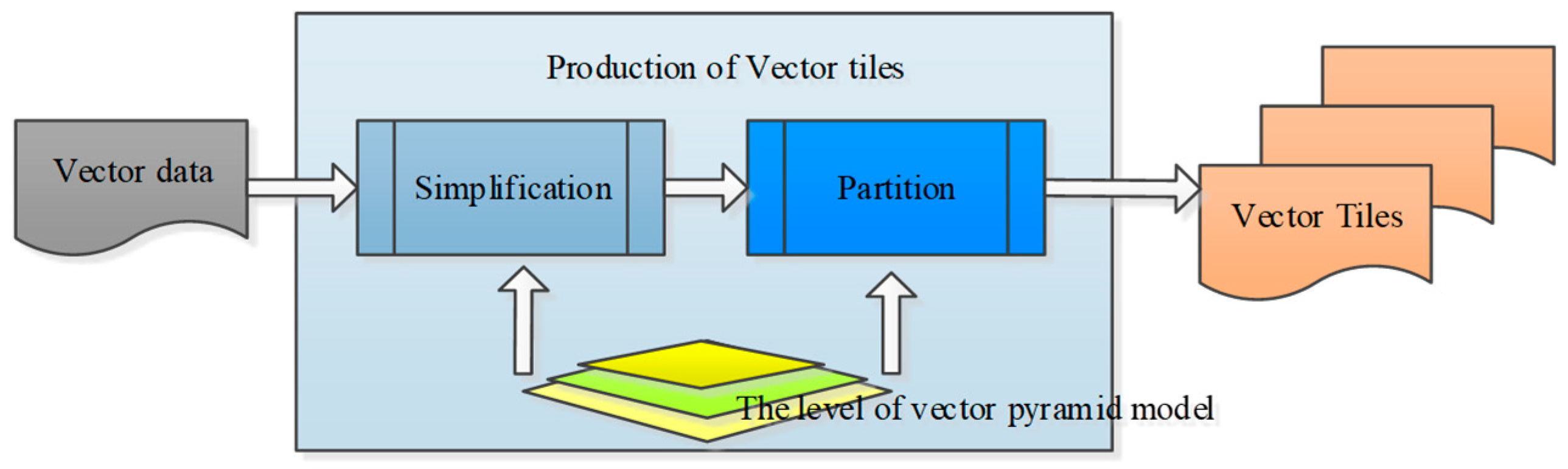
4. Construction of Vector Tiled Pyramid Model

Construction of the Vector Tiled Pyramid Model is a dynamic procedure that processes vector data into vector tiles. It includes two steps: stratification and partition. Stratification is the step that generates a level from the original vector data by simplification. Partitioning is the step that splits vector data into separate vector tiles.

As shown in Figure 2, vector tiles are produced level-by-level according to the level number in the VTPM. Vector data at each level is partitioned as tiles.

4.1. Vector Data Simplification

When vector data are visualized on a 3D terrain surface, redundant data do not play an active role in rendering since they increase the amount of data transmitted and slow down the process. Excessive redundant data leads to the repeated rendering of portions of the data on a terrain surface, reducing rendering efficiency. For example, a boundary line that contains dense node points creates excessive time costs when rendered in a 3D display. It is unnecessary to process all the node points for each level since many details will not be visible at this geographic scale. Therefore, simplification is essential to express vector data at different levels of detail.

Mantler proposed the concept of Safe Sets to handle complex, line vector data, to preserve the topological relations of vector data [32]. Based on this idea, Mustafa presented an algorithm that performs simplification on large geographical maps through a novel use of graphics hardware [33]. This algorithm uses the ε-Voronoi diagram to process vector data, which ensures that the two lines do not intersect after simplification. However, it cannot avoid the problem of self-intersection. Yang introduced the concept of monotone polylines to solve the problem of self-intersection [34]. Mustafa and Yang solved the problem of inconsistent topological relations before and after simplification; so, in this paper, we adopted their algorithms to simplify vector data. Specifically, a monotonous check pre-treatment is applied to ensure that all polylines are monotone and a simplification algorithm based on the ε-Voronoi diagram is adopted to simplify the vector data.

The simplification threshold is a key factor for the production of vector titles of different levels. At a given level of the VTPM, using an appropriate simplification threshold, a minimal subset, simultaneously without losing important feature information when the subset is visualized at the corresponding scales, can be produced from the original data.

Generally, the human eye cannot distinguish two points within the distance of one pixel on the screen. Therefore, in our experiment, the geographical distance corresponding to one pixel of the vector tile at different levels was selected as the simplification threshold for each level of the VTPM. Regardless of the rendering methods (texture-based methods and geometry-based methods), each vector tile is visualized on the screen with fixed size pixels, such as 256 × 256 or 512 × 512. The 256 × 256 sized pixels were adopted in our experiment. Thus the simplification threshold can be expressed as Equation (1).

$$\left\{\begin{array}{c}T=\left\{{\mathrm{t}}_1,{\mathrm{t}}_2,\dots ,{\mathrm{t}}_{\mathrm{N}}\right\} \\ {\mathrm{t}}_{\mathrm{n}}=\frac{\sqrt{\mathrm{S}}}{256{\ast \mathrm{R}}^{\mathrm{n}}} \left(\mathrm{n}=1,2,\dots ,\mathrm{N}\right)\end{array}\right.$$

(1)

where S represents the spatial range of the VTPM (Definition 1), N represents the number of levels of the VTPM (Definition 2), and R represents the ratio between the vector tiles at adjacent levels (Definition 3). T represents the simplification threshold for a VTPM (Definition 4). The t_n is the geographical distance corresponding to one pixel of the vector tile at level n of the VTPM and is the simplification threshold we adopted in our experiment.

4.2. Partition for Vector Data

In order to achieve block storage of vector data, vector data at each level are divided and stored in vector tiles. Each vector tile has a corresponding spatial extent. Point vector data can be stored into vector tiles by a simple overlay analysis using the coordinate ranges of the vector tiles. Polyline and polygon vector data must be partitioned so that they can be stored in their respective vector tiles.

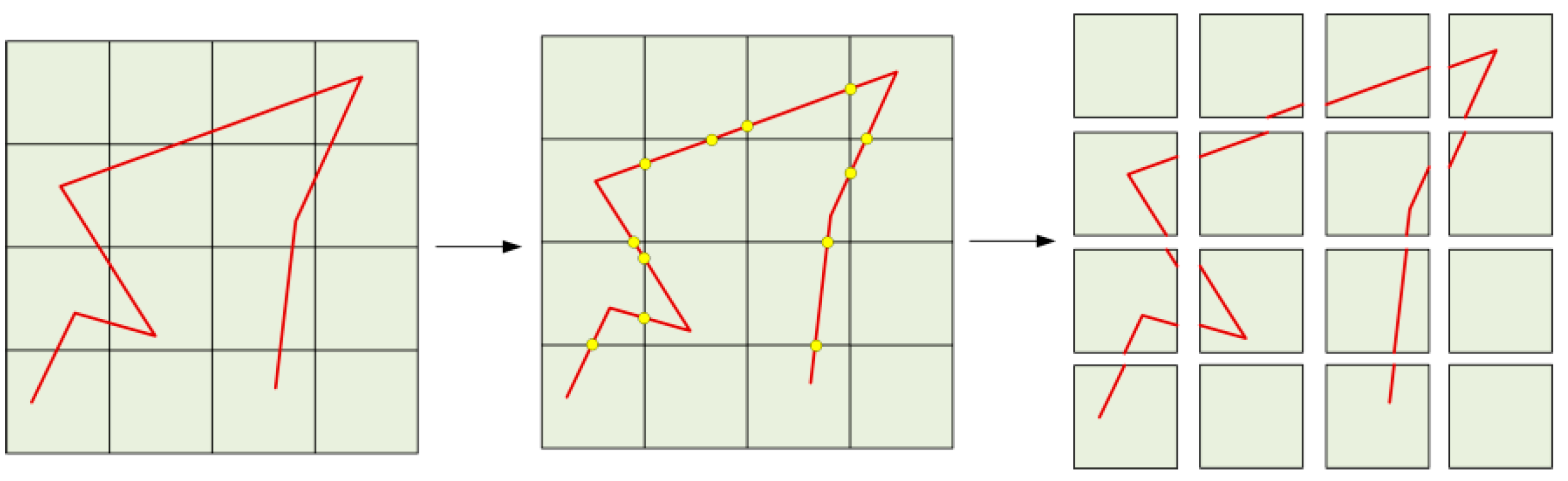
4.2.1. Segmentation of Polylines

In order to segment a polyline, we propose a point tracking method. As shown in Figure 3, starting with the beginning point of a polyline, the correspondence between each node of the polyline and vector tile is calculated. Vector data within the spatial range corresponding to the vector tile will be saved to the current vector tile.

The specific algorithm for the point tracking method is as follows:

• Step 1. For a polyline at a given level, first, find the coordinates of the starting point. Then, calculate the index number of the vector tile that includes the starting point.
• Step 2. Find the next point of the polyline, check if it still falls within the current vector tile. If so, then store the point in the current vector tile and continue the process with successive points until the next point is found to be out of the spatial extent of the current vector tile. Go to Step 3, if the next point does not fall inside the current vector tile.
• Step 3. Calculate the intersection point between the spatial extent of the current vector tile and the line segment formed by the current point and the last point. Save the coordinates of the intersection point to the current vector tile. Search among other vector tiles to find one that includes the intersection point and the successive points. Save the index number of this new vector tile and regard it as the current vector tile.
• Step 4. Take the intersection point as a new starting point and use the newly updated current vector tile, and repeat Steps 2 and 3 until all of the points of the vector line are processed.

The pseudocode for the point tracking algorithm is shown in Algorithm 1.

Algorithm 1: Segmentation Algorithm For Line Input: A Line l = {P1,…,Pn} Output: VectorTile

1 Current_VectorTile = CaculateVectorTile(P1) 2 Current_Segment = {P1} 3 foreach Pi (i > 1) in l do 4  if Pi in Current_VectorTile then 5     Current_Segment.Append(Pi) 6  else 7     P = CaculateIntersection() 8     Current_Segment.Append(P) 9     SaveVectorTile(Current_VectorTile, Current_Segment) 10   Current_VectorTile = CaculateVectorTile(P) 11   Current_Segment = {P} 12  end 13 end

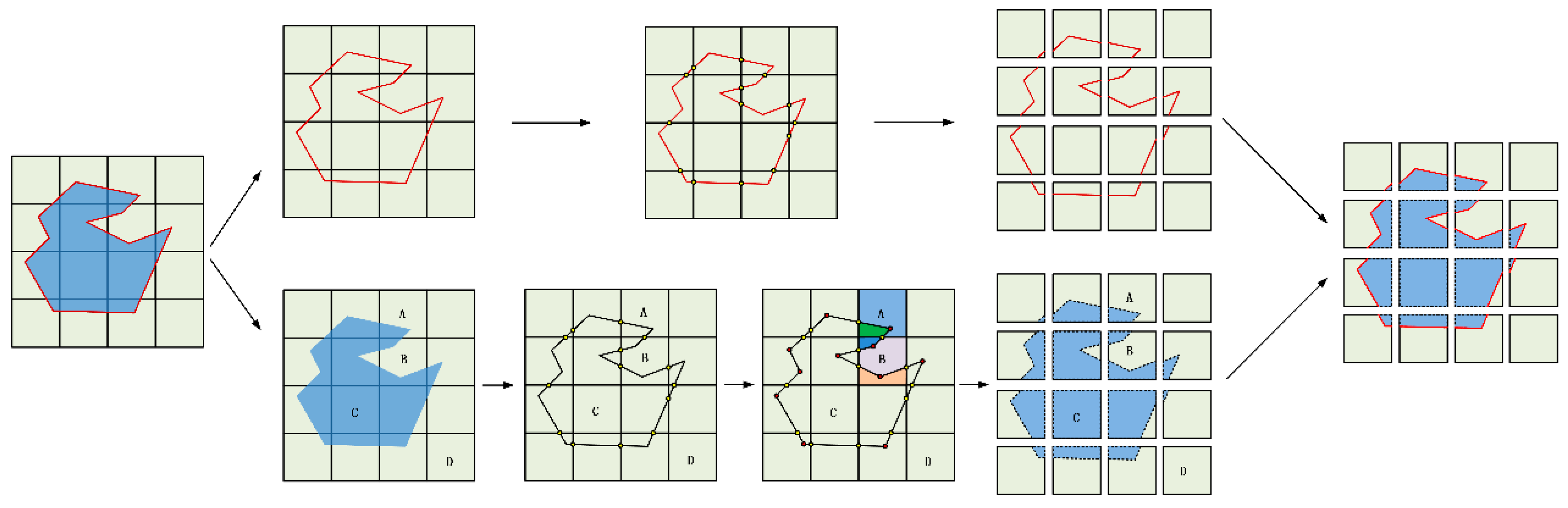
4.2.2. Segmentation of Polygons

The visualization of polygon vector data includes the interior fill and contour drawing approaches. In order to express polygon vector data completely, as shown in Figure 4, polygon vector data are divided into two parts (contour line and internal polygon), and these two parts are split and stored separately in a VTPM. The polyline segmentation algorithm (Algorithm 1) can be applied to the contour line segmentation, as shown in the upper half of Figure 4.

For internal polygon segmentation, we designed a tile tracking method, as shown in the lower half of Figure 4. There are two cases for the relationships between a vector tile and a polygon that we identify as cases one and two. In case one, there are edges of polygons in a vector tile, such as vector tiles A and B in Figure 4. In case two, there are no edges of polygons in a vector tile, such as vector tiles C and D. In case one, a vector tile is divided into two (vector tile A) or more portions (vector tile B); therefore, we need to individually determine the relationship between each portion and polygon. In case two, we need to determine if the spatial range corresponding to the vector tile belongs to the polygon (vector tile C) or the spatial range corresponding to the vector tile does not belong to the polygon (vector tile D).

Specifically, first, the intersection of an edge of a polygon and vector tile boundaries are calculated, and each vector tile was divided into one or several portions by these intersections and polygon nodes. Then, the relationship between each portion and the polygon was calculated. If a portion belongs to the polygon, then the portion is saved in the current vector tile. Eventually, polygons are split and stored in the corresponding vector tiles.

5. Experiment and Analysis

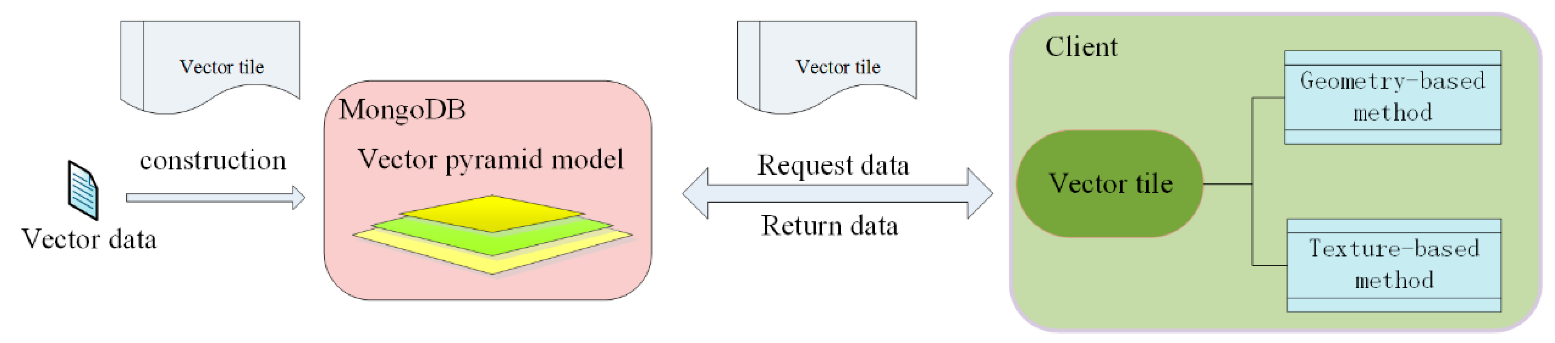
A prototype for the construction and 3D visualization for the VTPM was implemented in the way described in Figure 5. In the data pre-processing stage, we used the proposed VTPM construction algorithm to simplify and divide vector data as vector tiles. When displayed in 3D, the vector tiles are requested according to their index numbers at each level of the VTPM. After parsing vector tiles, either a geometry-based method or texture-based method can be used to render the vector data in 3D.

The MongoDB database was adopted to store the vector tiles in this experiment for two reasons. On the one hand, vector tiles store data objects in the form of key-value. The row and column number of each vector tile can be treated as the key, and then the vector data in the vector tile are the value corresponding to each key. The storage format of files in MongoDB is BSON, which supports key-value indexing. On the other hand, MongoDB is based on distributed file storage, which supports the expansion of data. The number of global vector data is very large, and it constantly increases; therefore, MongoDB was used to store the vector tiles.

There are two important processes in our prototype system. One is the production of vector tiles based on the VTPM, and the other is the visualization of vector tiles on a 3D terrain surface.

5.1. Production of Vector Tiles Based on the VTPM

We used four types of vector maps as our experimental data: the open source global administrative map, global rail polyline vector data, global road polyline vector data, and the lakes and woods polygon vector data for Wuhan, a large city in the inland central area of China, from the OpenStreetMap. The number of objects and vertices of each vector data are shown in

Table 1. Tested vector datasets.

Dataset Type	The Number of Objects	The Number of Vertices
global administrative map	746,615	43,597,863
global rail	1,204,816	14,346,928
global road	8,286,836	137,310,566
lakes and woods for Wuhan	730	46,826

.

A VTPM was described as followings for our experiment: since the experimental data are global, the global geographic scope was adopted as the spatial range of the VTPM (Definition 1); according to the experiment and formula 1, the number of levels of the VTPM is selected as seventeen, which is the most appropriate and can show more levels with different details (Definition 2); two was selected as the ratio between the vector tiles at adjacent levels (Definition 3); the Equation(1) mentioned in Section 4.1 was adopted as the simplification threshold of the VTPM (Definition 4). Based on the method mentioned in Section 4, we completed the construction of the VTPM for the experimental data.

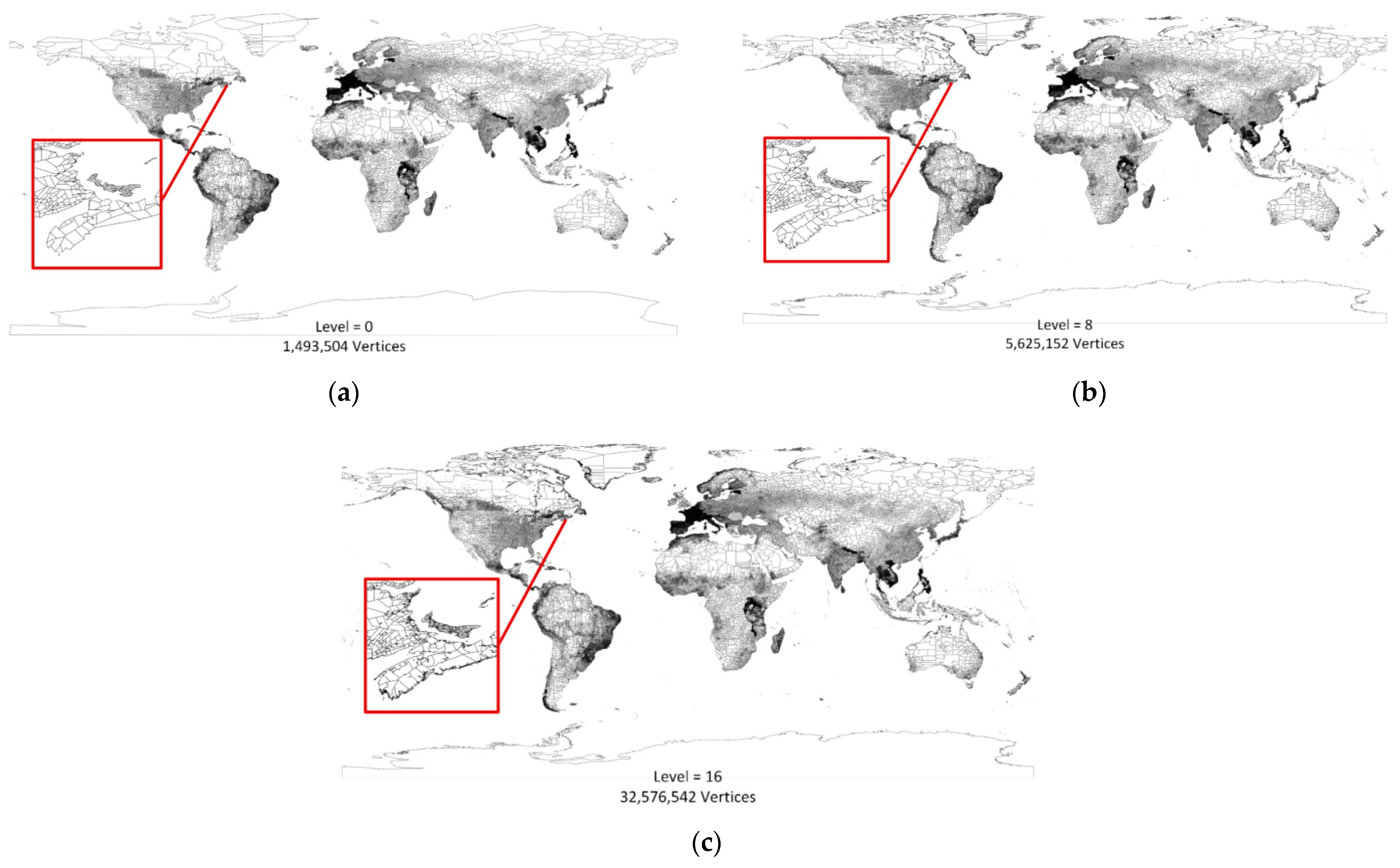
Figure 6a–c show the global administrative map at different levels. The numbers below each successive image represent the level number and the number of vertices of the vector tiles at that level of the VTPM.

From Figure 6, we can find that, based on the simplification scheme we adopted, the geometric features of the vector data at different levels are consistent and the details of the vector data change with the levels of the VTPM. The number of vertices in the vector tiles at different levels becomes larger with an increasing level number. Additionally, from the red rectangle in each subfigure, there are more and more details in the vector tiles with an increase in the level number.

Table 2. The number of vertices at different levels for global rail and global road.

Dataset Type	Level = 0	Level = 4	Level = 8	Level = 12	Level = 16
global rail	2,409,632	2,455,047	2,845,108	5,469,357	10,990,919
global road	16,573,675	16,883,297	20,636,291	41,489,263	106,503,532

shows the number of vertices in the vector tiles at different levels of the VTPM for the global rail and global road.

Table 3. The number of vertices at different levels for the lakes and woods for Wuhan.

Dataset Type	Level = 8	Level = 10	Level = 12	Level = 14	Level = 16
The lakes and woods for Wuhan	6692	11,359	18,279	27,486	42,222

shows the number of vertices in the vector tiles at different levels of the VTPM for the lakes and woods for Wuhan. The geographical scope of the city, such as Wuhan, is almost as large as the geographical scope of the vector tile at level eight of the VTPM in our experiment. So, we construct the vector tiles for the lakes and woods for Wuhan from level eight, not level zero.

5.2. Visualization of Vector Tiles on a 3D Terrain Surface

When displayed in 3D, vector tiles are requested according to the index number. After parsing vector tiles, either a geometry-based or texture-based method can be used to render the vector data in 3D. When a geometry-based approach is adopted to display the vector tile, elevation interpolation methods can be used to process the vector data into 3D coordinates. Further, 3D rendering techniques can then be used to visualize the vector data on a 3D terrain surface. When a texture-based approach is used to visualize the vector tiles, the vector tiles must be rasterized into texture vector tiles; texture mapping technology is used to map these texture vector tiles onto a 3D terrain surface.

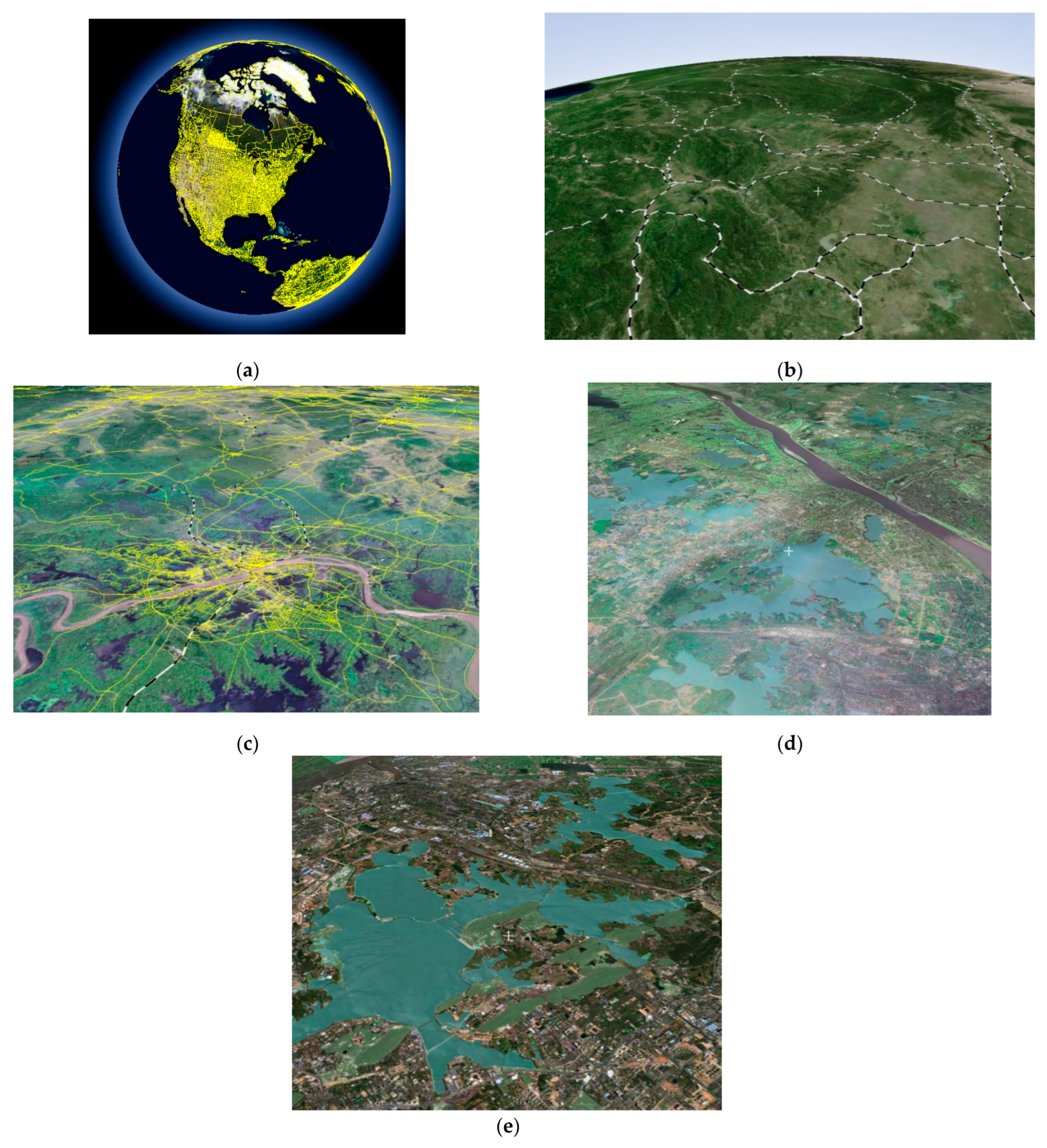
Supported by Geoglobal, a commercial software platform such as Google Earth, rendered vector data are shown in Figure 7. Figure 7a was created using a geometry-based method to visualize a global administrative map onto a global 3D terrain surface. In Figure 7b, a texture-based method was used to render the global rail data. Figure 7c shows vector data rendered using a combination of the two methods: a texture-based method for the global rail data, and a geometry-based method for global roads. Figure 7d,e show a visualization of the Wuhan lakes and woods polygon in 3D.

In our prototype system, when a texture-based approach is adopted to visualize the vector tiles, conventional map symbols can be combined with the rasterized vector data. For example, as shown in Figure 7b, conventional railway symbols are used to express the global rail vector data. Although there are no major technical problems when using the geometry-based method to express these simple map symbols, the low rendering efficiency detracts from the user experience, especially when dealing with global vector map data. So, in our experiment, we adopted a texture-based method to deal with the vector tiles when combining vector data with traditional map symbols.

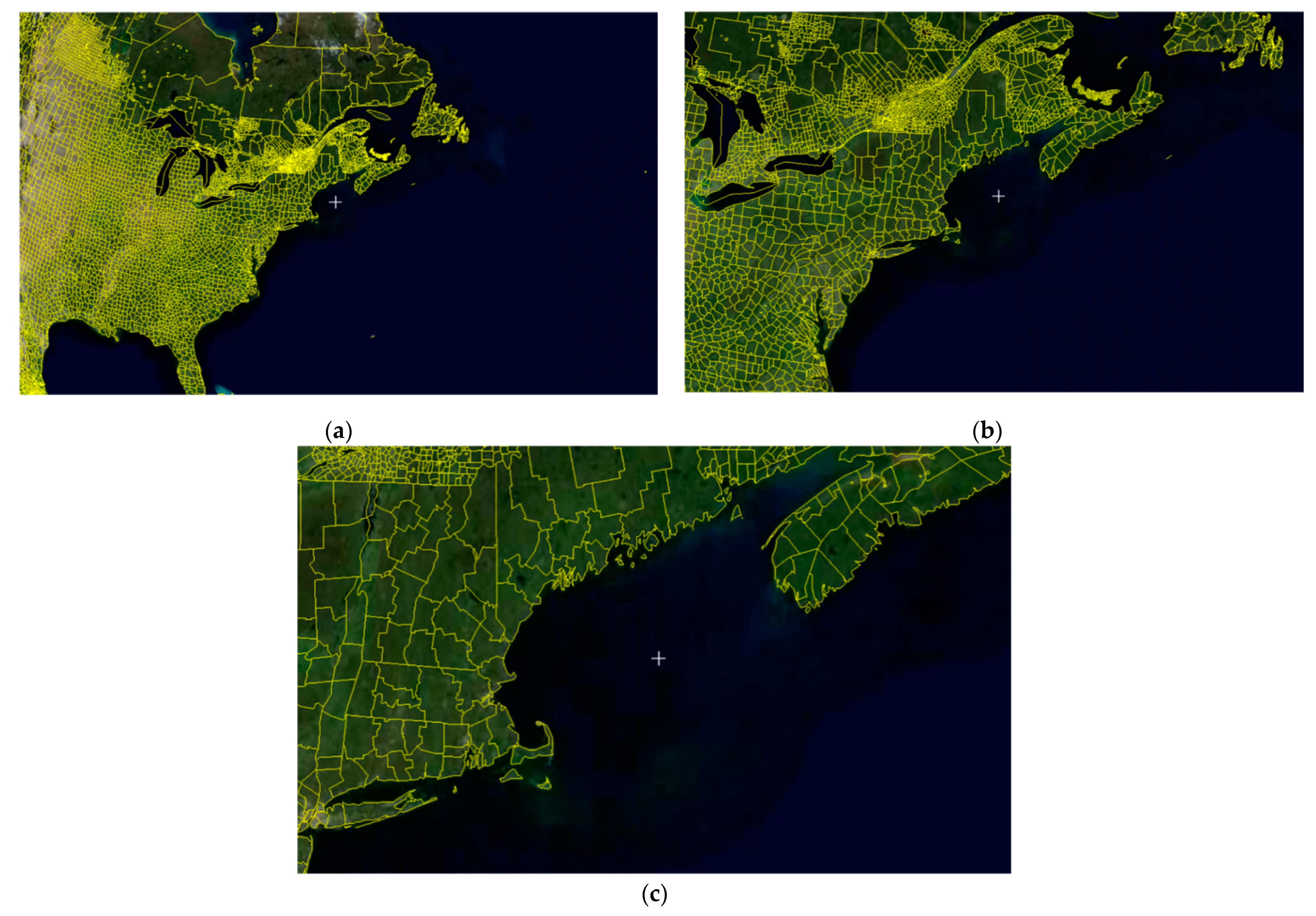
Figure 8 shows the 3D visualization of the vector tiles at different levels of the VTPM. When the perspective of the 3D scene is fixed, as shown in Figure 8a, the vector tiles within the current 3D scene will be requested and displayed. When a user zooms in, as shown in Figure 8b, the corresponding vector tiles at the lower levels of the VTPM will be requested and displayed on the 3D terrain surface. When zooming in further, as shown in Figure 8c, the vector tiles with more detail are requested. Figure 8a–c show the vector tiles at different levels of the VTPM.

5.3. Performance Analysis

The 3D visualization of vector data consists of two processes: obtaining requested data and rendering vector data. Therefore, the efficiency of obtaining requested data and the efficiency of rendering vector data are the two aspects of efficiency in the 3D representation of vector data. The efficiency when obtaining requested data depends on the organization and management of vector data.

In order to validate the efficiency of obtaining requested data based on the VTPM when rendering vector objects in 3D, a traditional vector database scheme and a VTPM for vector data were tested and compared. We used a PC with a 3.1 GHz Intel Core 3 CPU, 8 Gbytes of RAM for these tests of the two organizational schemes on the same vector data. We compared the performance time when obtaining requested data with the two organization schemes. If the time was short, then the efficiency of obtaining the requested data was higher.

In the VTPM, the size of vector tiles at different levels is not the same.

Table 4. The size of vector tiles corresponding to each level in the VTPM.

Level	0	1	2	3	4	...
Size (latitude × Longitude)	360 × 360	180 × 180	90 × 90	45 × 45	22.5 × 22.5	...

shows the size of vector tiles corresponding to each level in the VTPM in our experiment. Since the ratio between the vector tiles at adjacent levels (Definition 3) of the VTPM was two, as shown in Table 4, the size of the vector tile at the higher level is four times the size of the vector tile at the lower level.

In order to ensure that we obtained the same vector data objects at the same requested geographical scope in the two different organization schemes, we adopted a geographical scope corresponding to the vector tile in the VTPM as the geographical scope of the experimental request. From level zero to level nine of the VTPM, we successively selected a vector tile randomly and treated the geographical scope of the selected vector tile as the geographical scope of the experimental request, and we repeated this process 10,000 times.

Table 5. Comparing the two schemes for obtaining requested data.

	The Average Number of Objects per Request		The Average Number of Nodes per Request		The Average Time per Request (seconds)
Level	Traditional	VTPM	Traditional	VTPM	Traditional	VTPM	Ratio
0	746,651	746,651	43,597,863	1,493,498	15.8465	4.8173	3.28954
1	373,527	373,527	21,818,059	747,605	8.0957	2.3192	3.49068
2	102,367	102,367	6180,539	205,458	2.5555	0.6478	3.94471
3	40,028	40,028	2,242,651	81,065	1.1598	0.2489	4.65937
4	11,604	11,604	872,314	24,550	0.5683	0.0727	7.81463
5	2783	2783	265233	6819	0.3568	0.0179	19.941
6	1101	1101	94150	3248	0.5216	0.0077	68.0407
7	499	499	57105	1750	0.4176	0.0038	110.761
8	368	368	53738	1398	0.4333	0.0029	151.837
9	105	105	23646	668	0.2831	0.0014	205.586

illustrates our experimental results. The first column in the table shows different levels. The second and third columns in the table show the average number of objects of the acquired vector data per request based on the two schemes when the geographical scope corresponding to the vector tile at different levels of the VTPM was requested. The fourth and fifth columns show the average number of nodes of the acquired vector data per request based on the two schemes. The last three columns in the table show the average time per request based on the two schemes and the ratio of the average time of obtaining requested data between the two schemes.

As shown in Table 5, with an increasing number of levels, the number of objects and nodes of the vector data becomes less when the geographical scope corresponding to the vector tile at this level is requested. Accordingly, the time spent when obtaining requested data become less with increasing the number of the level.

The last column in Table 5 shows the ratio of the time of obtaining requested data based on the two schemes when the geographical scope corresponding to the vector tile at different levels of the VTPM was requested. It reflects the contrast in the efficiency between the two schemes. Overall, the efficiency of the VTPM is higher than the traditional vector database scheme. In addition, when the geographical scope of the vector tile at the lower levels of the VTPM was requested, the efficiency of the VTPM was significantly improved over the traditional vector database scheme, even up to hundreds of times. This reflects the block structure of the VTPM, which gradually plays a role in the efficiency of obtaining requested data with the increasing number of levels.

Therefore, using the VTPM to organize and manage vector data can improve the efficiency when visualizing vector data on 3D terrain surfaces by improving efficiency when obtaining requested data.

6. Conclusions

In this paper, we propose the VTPM for organizing and managing vector data. In the VTPM, vector data are stored at different levels with different details. These vector data at each level are divided into different blocks, and each block is considered a vector tile. This strategy will enhance the efficiency of visualizing vector data on 3D terrain surfaces.

In order to validate the utility of the VTPM, we designed and built a prototype system for visualizing vector data on 3D terrain surfaces based on the VTPM. The experimental results show that when compared with a traditional vector database, the VTPM enables fast access to vector data. This ensures efficiency when obtaining requested data for visualization on a 3D terrain. In addition, unlike the texture vector tiled pyramid, vector tiles in the VTPM are easily combined using a geometry-based approach or texture-based approach. We can even combine the two approaches to achieve a rich rendering effect. Therefore, the VTPM is a compromise solution that effectively visualizes vector data on 3D terrain surfaces, achieving a better balance between efficiency and effect.

It should be noted, however, that in the VTPM, the topology of the vector data is undermined due to the partitioning so spatial analysis of the vector data in VTPM is a problem. This problem will be addressed in our future work, possibly by building and incorporating a more extensive indexing structure to keep the topological relationships among vector objects.

References

- Alderson, T.; Purss, M.; Du, X.; Mahdavi-Amiri, A.; Samavati, F. Digital earth platforms. In Manual of Digital Earth; Springer: Singapore, 2020; pp. 25–54. [Google Scholar]
- Mahdavi-Amiri, A.; Alderson, T.; Samavati, F. A survey of digital earth. Comput. Graph. 2015, 53, 95–117. [Google Scholar] [CrossRef]
- Viaña, R.; Magillo, P.; Puppo, E.; Ramos, P.A. Multi-vmap: A multi-scale model for vector maps. Geoinformatica 2006, 10, 359–394. [Google Scholar] [CrossRef]
- Yang, B. A multi-resolution model of vector map data for rapid transmission over the Internet. Comput. Geosci. 2005, 31, 569–578. [Google Scholar] [CrossRef]
- Zhou, X.; Prasher, S.; Sun, S.; Xu, K. Multiresolution spatial databases: Making web-based spatial applications faster. In Advanced Web Technologies and Applications; Springer: Berlin/Heidelberg, Germany, 2004; pp. 36–47. [Google Scholar]
- Ottoson, P.; Hauska, H. Ellipsoidal quadtrees for indexing of global geographical data. Int. J. Geogr. Inf. Sci. 2002, 16, 213–226. [Google Scholar] [CrossRef]
- Kersting, O.; Döllner, J. Interactive 3D visualization of vector data in GIS. In Proceedings of the 10th ACM International Symposium on Advances in Geographic Information Systems, McLean, VA, USA, 8–9 November 2002. [Google Scholar]
- Schneider, M.; Klein, R. Efficient and accurate rendering of vector data on virtual landscapes. J. WSCG 2007, 15, 59–64. [Google Scholar]
- Tanimoto, S.; Pavlidis, T. A hierarchical data structure for picture processing. Comput. Graph. Image Process. 1975, 4, 104–119. [Google Scholar] [CrossRef]
- Walker, P.A.; Grant, I.W. Quadtree: A FORTRAN program to extract the quadtree structure of a raster format multicolored image. Comput. Geosci. 1986, 12, 401–409. [Google Scholar] [CrossRef]
- Song, X.; Neuvo, Y. Image compression using nonlinear pyramid vector quantization. Multidimens. Syst. Signal Process. 1994, 5, 133–149. [Google Scholar] [CrossRef]
- Lin, H. A pyramid algorithm for fast fractal image compression. In Proceedings of the 1995 International Conference Image Processing, Washington, DC, USA. 23–26 October 1995. [Google Scholar]
- Cline, D.; Egbert, P.K. Interactive display of very large textures. In Proceedings of the Visualization’98, Blaubeuren, Germany, 20–22 April 1998; IEEE: Piscataway, NJ, USA, 1998; pp. 343–350. [Google Scholar]
- Goss, M.E.; Yuasa, K. Texture tile visibility determination for dynamic texture loading. In Proceedings of the ACM SIGGRAPH/EUROGRAPHICS Workshop on Graphics Hardware, Lisbon, Portugal, 31 August–1 September 1998. [Google Scholar]
- Döllner, J.; Baumman, K.; Hinrichs, K. Texturing techniques for terrain visualization. In Proceedings of the Conference on Visualization’00, Salt Lake City, UT, USA, 8–13 October 2000; IEEE Computer Society Press: Piscataway, NJ, USA; ACM: Cambridge, MA, USA, 2000; pp. 227–234. [Google Scholar]
- Olanda, R.; Pérez, M.; Orduña, J.M.; Rueda, S. Terrain data compression using wavelet-tiled pyramids for online 3D terrain visualization. Int. J. Geogr. Inf. Sci. 2014, 28, 407–425. [Google Scholar] [CrossRef]
- Atta, R.; Ghanbari, M. Low-contrast satellite images enhancement using discrete cosine transform pyramid and singular value decomposition. IET Image Process. 2013, 7, 472–483. [Google Scholar] [CrossRef]
- Binaghi, E.; Gallo, I.; Pepe, M. A cognitive pyramid for contextual classification of remote sensing images. IEEE Trans. Geosci. Remote Sens. 2003, 41, 2906–2922. [Google Scholar] [CrossRef]
- Goffe, R.; Brun, L.; Damiand, G. Tiled top–down combinatorial pyramids for large images representation. Int. J. Imaging Syst. Technol. 2011, 21, 28–36. [Google Scholar] [CrossRef] [Green Version]
- Reddy, M.; Leclerc, Y.; Iverson, L.; Bletter, N. TerraVision II: Visualizing massive terrain databases in VRML. Comput. Graph. Appl. 1999, 19, 30–38. [Google Scholar] [CrossRef]
- Schmidt, C.R.; Dev, B. A Scalable Tile Map Service for Distributing Dynamic Choropleth Maps; Working Paper; GeoDa Center for Geospaital Analysis and Computation; Arizona State University: Tempe, AZ, USA, 2008. [Google Scholar]
- Haklay, M.; Weber, P. Openstreetmap: User-generated street maps. Pervasive Comput. 2008, 7, 12–18. [Google Scholar] [CrossRef] [Green Version]
- Maso, J.; Pomakis, K.; Julia, N. OpenGIS Web Map Tile Service Implementation Standard; Open Geospatial Consortium Inc.: Rockville, MD, USA, 2010; pp. 4–6. [Google Scholar]
- Agrawal, A.; Radhakrishna, M.; Joshi, R.C. Geometry-based mapping and rendering of vector data over LOD phototextured 3D terrain models. In Proceedings of the WSCG 2006—The 14th International Conference in Central Europe on Computer Graphics, Visualization and Computer Vision, Plzen-Bory, Czech Republic, 30 January–3 February 2006. [Google Scholar]
- Wartell, Z.; Kang, E.; Wasilewski, T.; Ribarsky, W.; Faust, N. Rendering vector data over global, multi-resolution 3D terrain. In Proceedings of the Symposium on Data Visualisation 2003, Eurographics Association, Grenoble, France, 26–28 May 2003. [Google Scholar]
- Bruneton, E.; Neyret, F. Real Time Rendering and Editing of Vector based Terrains. In Computer Graphics Forum: Eurographics; Blackwell Publishing Ltd.: Crete, Greece, 2008; Volume 27, pp. 311–320. [Google Scholar]
- Sun, M.; Lv, G.; Lei, C. Large-scale vector data displaying for interactive manipulation in 3D landscape map. Int. Arch. Photogramm. Remote Sens. Spat. Inf. Sci. 2008, 37, 507–511. [Google Scholar]
- Chew, L.P. Constrained delaunay triangulations. Algorithmica 1989, 4, 97–108. [Google Scholar] [CrossRef]
- Qi, M.; Cao, T.T.; Tan, T.S. Computing 2D constrained Delaunay triangulation using the GPU. IEEE Trans. Vis. Comput. Graph. 2013, 19, 736–748. [Google Scholar] [CrossRef]
- Douglas, D.H.; Peucker, T.K. Algorithms for the reduction of the number of points required to represent a digitized line or its caricature. Cartogr. Int. J. Geogr. Inf. Geovis. 1973, 10, 112–122. [Google Scholar] [CrossRef] [Green Version]
- Shi, W.; Cheung, C.K. Performance evaluation of line simplification algorithms for vector generalization. Cartogr. J. 2006, 43, 27–44. [Google Scholar] [CrossRef]
- Mantler, A.; Snoeyink, J. Safe sets for line simplification. In Proceedings of the 10th Annual Fall Workshop on Computational Geometry, New York, NY, USA, 27–28 October 2000. [Google Scholar]
- Mustafa, N.; Krishnan, S.; Varadhan, G.; Venkatasubramanian, S. Dynamic simplification and visualization of large maps. Int. J. Geogr. Inf. Sci. 2006, 20, 273–302. [Google Scholar] [CrossRef]
- Yang, L.; Zhang, L.; Ma, J.; Kang, Z.; Zhang, L.; Li, J. Efficient Simplification of Large Vector Maps Rendered onto 3D Landscapes. IEEE Comput. Graph. Appl. 2011, 31, 14–23. [Google Scholar] [CrossRef] [PubMed]