Improvement of Oracle Bone Inscription Recognition Accuracy: A Deep Learning Perspective

Abstract

Deep learning techniques have been successfully applied in handwriting recognition. Oracle bone inscriptions (OBI) are the earliest hieroglyphs in China and valuable resources for studying the etymology of Chinese characters. OBI are of important historical and cultural value in China; thus, textual research surrounding the characters of OBI is a huge challenge for archaeologists. In this work, we built a dataset named OBI-100, which contains 100 classes of oracle bone inscriptions collected from two OBI dictionaries. The dataset includes more than 128,000 character samples related to the natural environment, humans, animals, plants, etc. In addition, we propose improved models based on three typical deep convolutional network structures to recognize the OBI-100 dataset. By modifying the parameters, adjusting the network structures, and adopting optimization strategies, we demonstrate experimentally that these models perform fairly well in OBI recognition. For the 100-category OBI classification task, the optimal model achieves an accuracy of 99.5%, which shows competitive performance compared with other state-of-the-art approaches. We hope that this work can provide a valuable tool for character recognition of OBI.

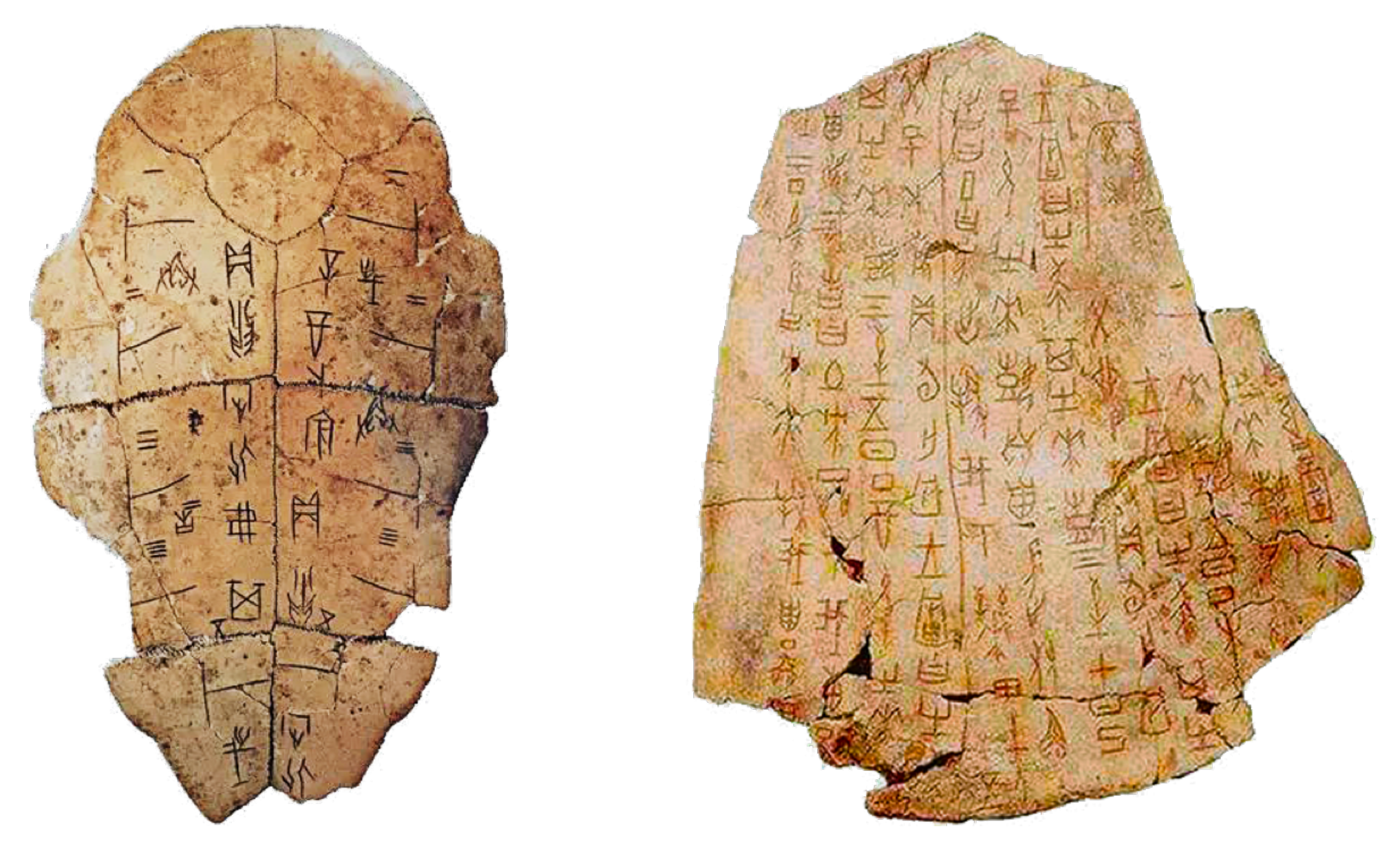
1. Introduction

Oracle bone inscriptions (OBI) were recorded from as early as the Shang Dynasty in China [1]. The script involves some of the oldest characters in the world and the earliest known form of characters in China and East Asia. The characters of OBI have a profound impact on the formation and development of Chinese characters, which are usually engraved on animal bones or tortoise shells for the purpose of pyromantic divination [2,3,4], as shown in Figure 1.

Figure 1. The abdominal parts of two tortoise shells with divinatory inscriptions excavated at the site of Yinxu, Anyang, Henan, China.

Figure 2a shows the characters of OBI corresponding to some commonly used words today. We can see that characters of OBI were written by drawing shapes and lines based on the shape features of objects, which was one of the most primitive methods of pictographs used by ancient people. To date, archaeologists have discovered more than 4500 characters of OBI, but the meanings of half of these characters have not yet been identified [5]. In the past, experts used manual comparison and analysis to identify the meaning of the characters of OBI based on existing experience, which was effective, but required time and effort. In addition, since characters of OBI were carved by different groups of ancient people from several historical periods [2], the characters had large variations in shape, scale, and orientation. For instance, the eight characters shown in Figure 2b have very similar glyphs, but represent eight words with very different meanings. On the contrary, Figure 2c shows eight characters of OBI written in various ways, however, they all express the same meaning of monkey. These pose huge challenges in recognizing characters of OBI.

Figure 2. Examples of OBI characters. (a) Examples of characters of OBI corresponding to eight commonly used words. (b) Eight characters of OBI that have different meanings, but look very similar. (c) Eight writing styles of monkey in OBI.

Recently, some automated methods for identifying OBI were proposed, among which, feature extraction is the most commonly used. Dress Andreas et al. [6] presented an analysis of oracle bone characters for animals from a cognitive point of view. Yang [7] proposed a graph theory to identify OBI, whose core idea was to regard an inscription character as an undirected graph and extract the topological characteristics for recognition. In Li et al.’s work [8], a human–computer interactive dynamic description method was proposed, which described OBI by the stroke–segments–vector and the stroke elements. A Fourier descriptor based on a curvature histogram (FDCH) was proposed by Lu et al. [9] to represent oracle characters. Gu [10] converted the OBI into topological figures and encoded the topographic figures. Meng [11,12] used the Hough transform to extract line features of characters of OBI, resulting in an inscription recognition accuracy of nearly 90%. Although feature extraction-based approaches can achieve the purpose of identifying characters of OBI, they are only suitable for simple data types or small datasets.

Artificial intelligence (AI) technology has strong potential in OBI recognition, and some researchers applied pattern recognition and deep learning to the recognition tasks. Support vector machine (SVM) [13,14] classification technology was used to recognize characters of OBI and reach an accuracy of 88%. Gao et al. [15] used the Hopfield network for recognizing fuzzy characters of OBI and the highest accuracy rate was 82%. Guo et al. [3] proposed a novel hierarchical representation that combined a Gabor-related low-level representation and a sparse-encoder-related mid-level representation; they combined this method with convolutional neural networks (CNNs) and achieved 89.1% accuracy in recognition. Although OBI recognition technologies based on deep learning have good scalability on large datasets, an overall recognition accuracy still needs to be improved. In this paper, we explore new approaches to improve the accuracy of OBI recognition using CNNs. Our major contributions are summarized as follows:

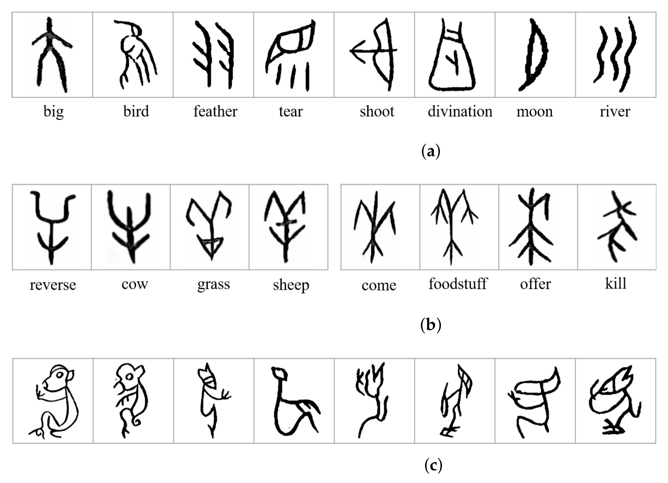
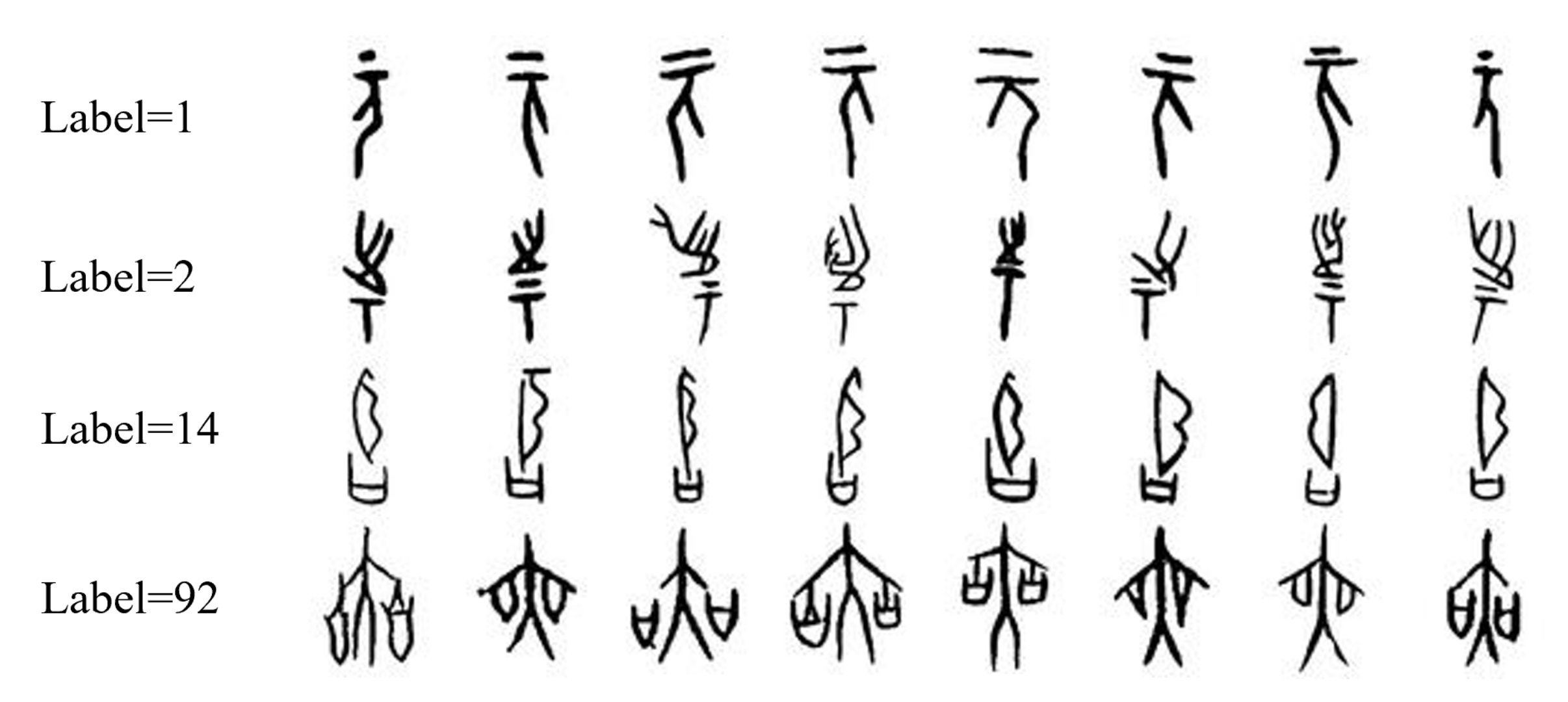
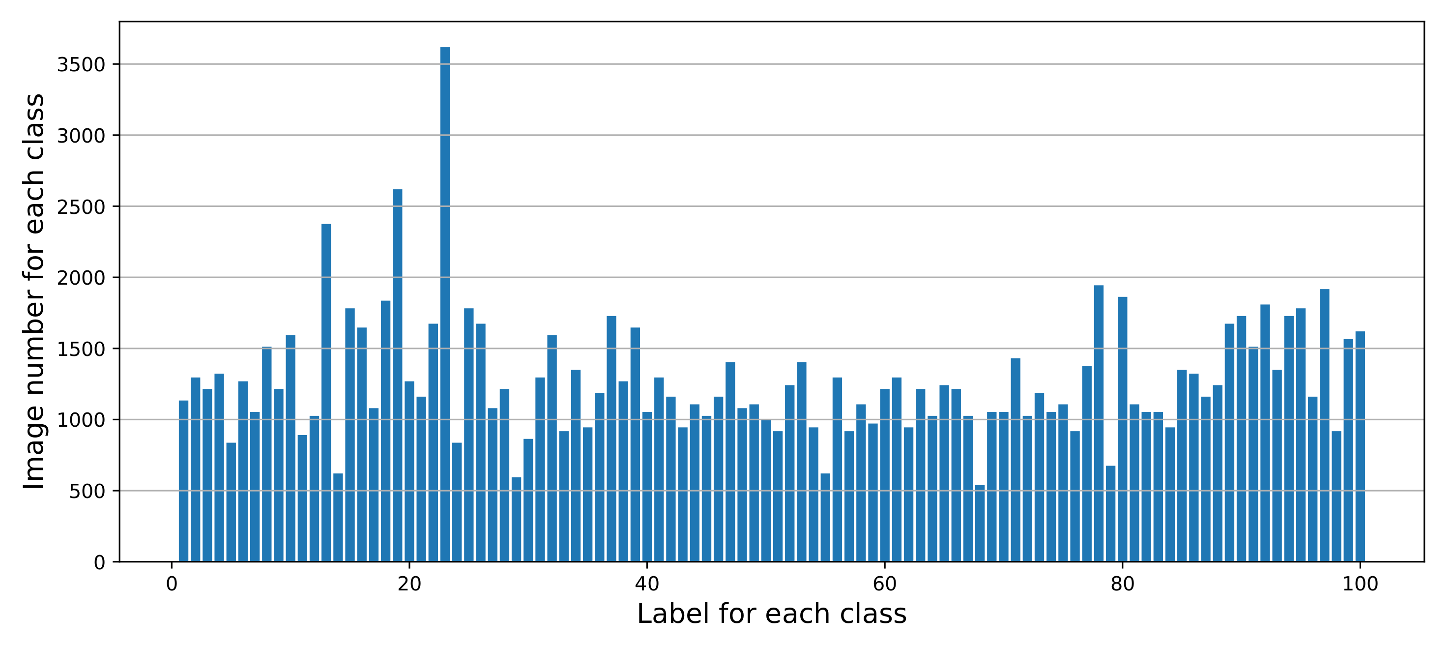
• We created a dataset named OBI-100 with 100 classes characters of OBI, covering various types of characters, such as animals, plants, humanity, society, etc., with a total of 4748 samples. Each sample in the dataset was selected carefully from two definitive dictionaries [16,17]. In view of the diversity of ancient OBI writing styles, we also used rotation, resizing, dilation, erosion, and other transformations to augment the dataset to over 128,000 images. The original dataset can be found at https://github.com/ShammyFu/OBI-100.git (accessed on 10 December 2021).
• Based on the convolutional neural frameworks of LeNet, AlexNet, and VGGNet, we produced new models by adjusting network parameters and modify network layers. These new models were trained and tested with various optimization strategies. From hundreds of different model attempts, ten CNN models with the best performance were selected to identify the 100-class OBI dataset.
• The proposed models achieved great recognition results on the OBI dataset, with the highest accuracy rate of 99.5%, which is better than the three classic network models and better than other methods in the literature.

2. Materials and Methods

2.1. Dataset Preparation

2.1.1. Sample Acquisition

Since characters of OBI are carved on tortoise shells and animal bones, people generally save them as paper or electronic sample collections by rubbing or taking pictures. The raw data in our dataset come from two classic scanned OBI dictionaries [16,17], both of which are definitive in the field of OBI.

The original dataset contains 100 classes of oracle character samples, of which the smallest category contains 20 samples, and the largest class has 134 examples, with a total of 4748 character images. In order to ensure the diversity of the dataset, the character categories we select cover humanities, animals, plants, natural environment and activities, etc. Besides, considering that some characters of OBI have many non-standard variants, we select as many of these characters as possible to ensure that the dataset is closer to the reality. This dataset is named OBI-100. After doing this part of the original data collection, we enhance the completeness and diversity of the dataset through preprocessing, augmentation, and normalization.

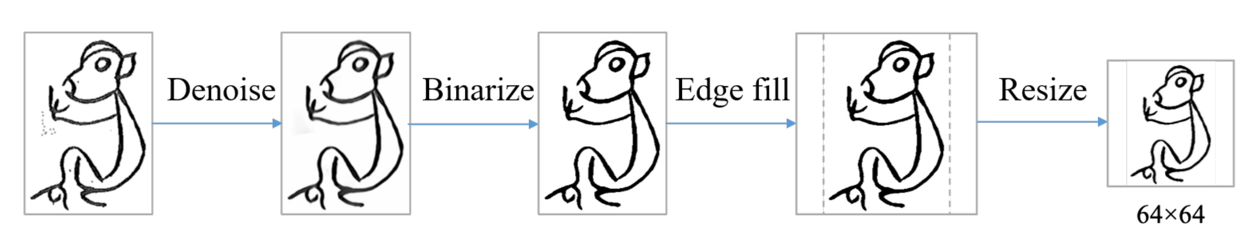
2.1.2. Dataset Preprocessing

To restore the writing characteristics of OBI more accurately, we preprocess the original samples as shown in Figure 3.

Figure 3. The preprocessing process of OBI character “monkey”.

• Denoising: since the OBI samples are from scanned e-books, Gaussian noise was introduced in the images. We first chose the non-local method (NLM) [18] to denoise. For a pixel in an image, this method finds similar regions of that pixel in terms of image blocks, and then averages the pixel values in these regions, and replaces the original value of this pixel with the average value [19], which can effectively eliminate Gaussian noise.
• Binarization: since the OBI images used for recognition require only black and white pixel values, we converted the denoised samples into grayscale ones and then binarized them.
• Size normalization: to keep the size of all images consistent without destroying the useful information areas of them, we rescaled the size of the image to $64\times 64$. For the original non-square images, we filled the blank edge area with white pixels first and then scaled them to the required size.

We show examples of the preprocessed dataset in Figure 4.

Figure 4. Examples of OBI-100 dataset.

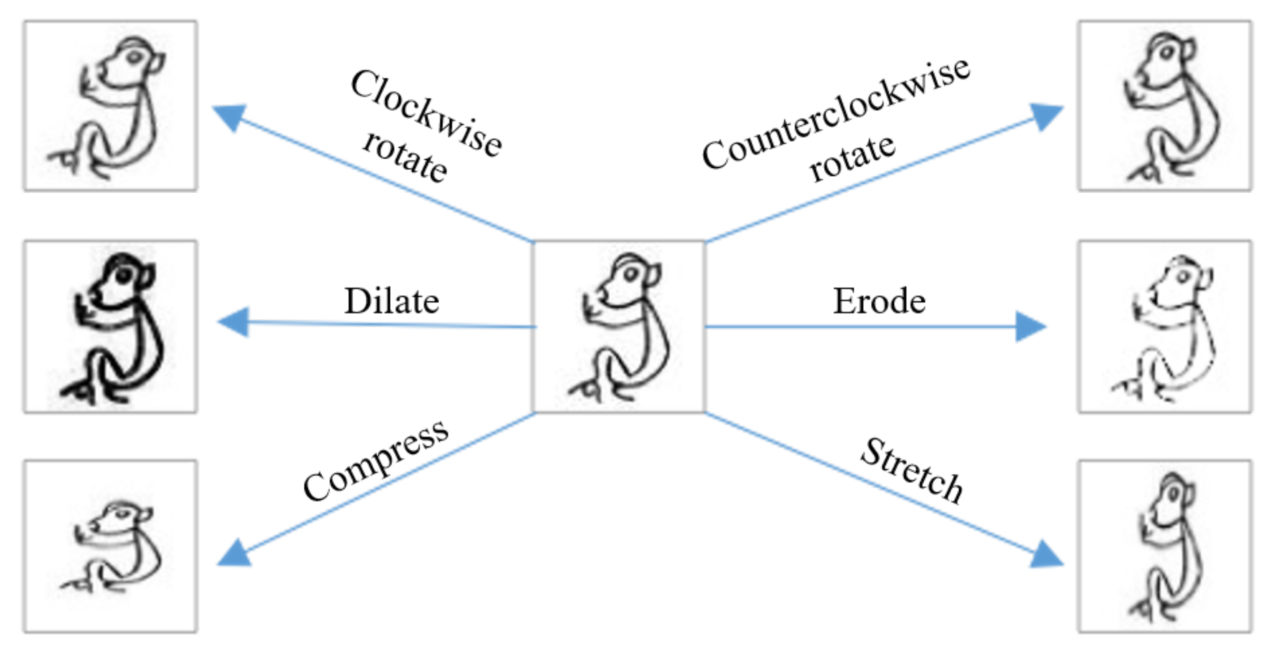
2.1.3. Data Augmentation

The insufficient number of samples in the dataset leads to low recognition accuracy, so we expand the dataset to improve the effectiveness of the recognition task. Considering the randomness of the same character when it is written multiple times, the angle or thickness of the character writing may change. Therefore, we perform several transformations to produce new images, as shown in Figure 5 for each sample.

Figure 5. An instance of data augmentation.

• Rotation: generate new images by rotating the original images clockwise or counterclockwise. The rotation angle is randomly selected from 0 to 15 degrees.
• Compress/stretch: adjust the shape of the characters on images by stretching or compressing, using a stretching ratio of 1 to 1.5, and a compression ratio of 0.67 to 1. The deformed images are rescaled to $64\times 64$.
• Dilation/erosion: dilate or erode the lines of characters of OBI [20] to produce new samples. Due to the small image size, direct corrosion will cause the loss of many features. We first enlarged the image, then implemented the corrosion operation, and finally resized the image size to $64\times 64$ to obtain the best corrosion effect.
• Composite transformation: in addition to the six individual transformations described above, we also apply twenty combinations of transformations to the samples. That is, the image is transformed several times by choosing two or more of the above methods to generate the corresponding new samples.

After the augmentation operation, each original image produces 26 corresponding transformed images. The total number of samples increased by 27 times to 128,196 ($4748\times 27$). The smallest class contains about 540 images and the largest category has over 3600 images. It presents the number distribution of each category in the OBI dataset in Figure 6.

Figure 6. The number of samples in each category of the augmented OBI-100 dataset.

2.2. Models Preparation

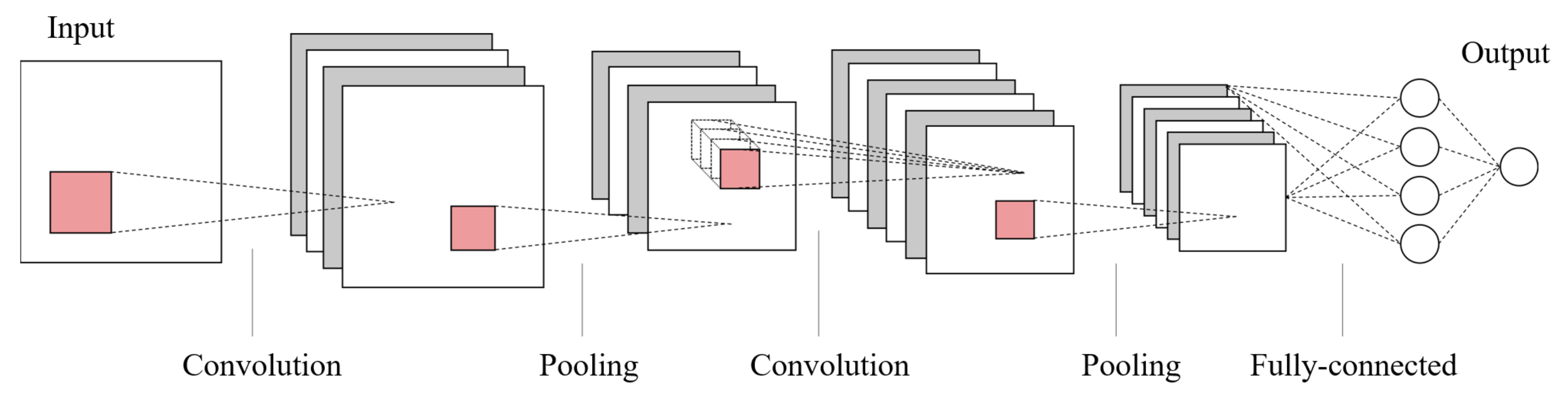
2.2.1. Background of CNN

Convolutional neural network (CNN) [21] is a multi-layer feed-forward neural network that can extract features and properties from the input data. Currently, CNN plays an important role in deep learning, because it can learn nonlinear mappings from a very large number of data (images or sounds), even in high-dimensional complex inputs. In addition, the capability of representation learning enables a CNN to classify input information according to its hierarchical structure by translation invariant classification. Specifically, a trained CNN can transform the original image at each layer of the network to produce a class score corresponding to that input image at the end of the network [22].

Generally, as shown in Figure 7, the basic CNN structure consists of an input layer, several convolutional layers, and pooling layers, as well as several fully connected layers and an output layer.

Figure 7. The basic structure of CNN.

The convolutional layer is designed to extract features from the input data, which contain many convolutional kernels. Each element of the kernel corresponds to a weight coefficient and a bias vector. The parameters of the convolutional layer include the size of the kernel, the step size, and the padding method [23]. These three factors jointly determine the size of the output feature map of the convolutional layer [24]. By introducing an activation function, CNN can effectively solve various nonlinear problems. The activation function maintains and maps the features of the activated neuron to the next layer. Typically, CNNs use the linear rectifier function (rectified linear unit, ReLU) [25] as the activation function to help express complex features, which can be formulated as $ReLU\left(x\right)=max(0,x)$. After feature extraction [26] by the convolutional layer, the output feature map is transferred into the pooling layer for feature selection and information filtering. The pooling layer actually implements the sampling function, and its main idea is to extract features with a certain tendency. For example, max pooling corresponds to more prominent features, while average pooling corresponds to smoother features. The fully connected layer combines the extracted features in a linear manner to get the output. The output layer uses a logistic function or a normalized exponential function to output the classification label or probability. Usually, the softmax function [27] is used to calculate the class scores as follows:

$$L_i=-log\frac{e^{f_{y_i}}}{{\sum }_j{e}^j}.$$

In the choice of network structure, we trained several mainstream models on the OBI-100 dataset, including LeNet, AlexNet, VGGNet, ResNet-50, and Inception. However, after preliminary experiments, it was found that the results of ResNet-50 and Inception are not satisfactory (their accuracy rates are both less than 70%). Therefore, we selected three network frameworks with stronger performance and higher training efficiency: LeNet, AlexNet, and VGGNet. Based on these three models, we adjusted the network structure, modified the parameters, and used various optimization methods to find models with better performance. After trying hundreds of combinations, we selected ten models that performed well. Table 1 summarizes the configuration of these ten improved models.

Table 1. Convolutional neural network configurations. Input: gray-scale images with a size of $64\times 64$ from OBI-100. Conv x-y: a convolutional layer with a kernel size of $x\times x$ and an output dimension of the feature map of y. FC-y: a fully connected layer with an output dimension of the feature map of y; maxpool: $m\times m$: a max pooling layer with a kernel size of $m\times m$. All network models use ReLU as the activation function and use softmax to calculate cross entropy loss.

ConvNet Configurations
Framework	LeNet		AlexNet			VGGNet
Name of our proposed Models	L1	L2	A1	A2	A3	V11	V13	V16	V16-2	V19
Input	$64\times 64$ gray-scale images from OBI-100.
Network Structure	conv5-6	conv3-32	conv11-64	conv11-64	conv11-64	conv3-64 conv3-64	conv3-32 conv3-32	conv3-64 conv3-64	conv3-64 conv3-64	conv3-64 conv3-64 conv3-64
	maxpool: $2\times 2$		maxpool: $3\times 3$	maxpool: $2\times 2$		maxpool: $2\times 2$
	conv5-16	conv5-64	conv5-192	conv5-192	conv5-192	conv3-128 conv3-128	conv3-64 conv3-64	conv3-64 conv3-64	conv3-64 conv3-64	conv3-128 conv3-128 conv3-128
	maxpool: $2\times 2$		maxpool: $3\times 3$	maxpool: $2\times 2$		maxpool: $2\times 2$
			conv3-384 conv3-256	conv3-384 conv3-256 conv3-256	conv3-384 conv3-256 conv3-256	conv3-256 conv3-256	conv3-128 conv3-128	conv3-128 conv3-128 conv3-128	conv3-128 conv3-128 conv1-128	conv3-256 conv3-256 conv3-256
			maxpool: $3\times 3$	maxpool: $2\times 2$		maxpool: $2\times 2$
				conv3-256 conv3-256	conv3-512 conv3-1024 conv3-1024	conv3-512 conv3-512	conv3-256 conv3-256	conv3-256 conv3-256 conv3-256	conv3-256 conv3-256 conv1-256	conv3-512 conv3-512 conv3-512
					maxpool: $2\times 2$	maxpool: $2\times 2$
							conv3-512 conv3-512	conv3-512 conv3-512 conv3-512	conv3-512 conv3-512 conv1-512	conv3-512 conv3-512 conv3-512 conv3-512
							maxpool: $2\times 2$
	FC-120	FC-512	FC-4096 FC-4096	FC-1024 FC-1024	FC-4096 FC-4096	FC-4096 FC-4096	FC-4096 FC-4096	FC-4096 FC-4096	FC-1024 FC-1024	FC-4096 FC-4096
	FC-100
	softmax

2.2.2. The Improved LeNet Models

LeNet [28] is one of the most representative models for handwritten digit recognition. It consists of two parts: (i) a convolutional encoder consisting of two convolutional layers and two pooling layers; (ii) a dense block consisting of three fully connected layers. For OBI classification tasks, we propose two improved models based on LeNet, called L1 and L2. For the two models, we adjusted the original seven-layer structure to a six-layer structure, and adjusted the depth of the convolutional layer and the size of the filter. Specifically, the output dimensions of the convolutional layers and the fully connected layers of the L1 model are basically the same as the original LeNet model, but the 120-depth fully connected layer is directly connected to the last 100-depth fully connected layer. On the L2 model, we used a higher-dimensional convolution kernel. For example, the first convolutional layer uses a 32-dimensional $3\times 3$ convolution kernel, and the second convolutional layer uses a 64-dimensional $5\times 5$ convolution kernel. In addition, the max pooling method is used in both models. We set the padding parameters of the L1 convolutional layers to the VALID value, which means that the size of the output feature map will change after convolution. However, the corresponding parameters of the L2 model are set to SAME, which means that the image size remains unchanged after convolution. Through these adjustment strategies, the L1 model inputs 16 feature maps with a size of $13\times 13$ to the fully connected layer, and L2 inputs 64 feature maps with a size of $16\times 16$.

2.2.3. The Improved AlexNet Models

AlexNet [25] is the winning model in the 2012 ImageNet competition, which consists of five convolutional layers, three max-pooling layers, two batch normalization layers, two fully connected layers, and one softmax layer. For AlexNet, we propose three optimized networks to classify characters of OBI, named A1, A2, and A3. These three models have different numbers of convolutional layers and pooling layers, and the first four convolutional layers have exactly the same structure. Specifically, the A2 model has three more convolutional layers with 256-dimensional $3\times 3$ convolution kernels and a pooling layer than the A1 model. Compared with the A2 model, the A3 model not only improves the depth of the network, but also uses higher-dimensional convolution kernels. In addition, we use the max pooling strategy for all networks. The max pooling layers in the A1 model use $3\times 3$ kernels, while those in the A2 and A3 models use $2\times 2$ kernels. In A1 and A3, the pooling layer is added between the last convolutional layer and the fully connected part, whereas the last convolutional layer of the A2 model is directly connected to the first fully connected layer.

2.2.4. The Improved VGGNet Models

Like AlexNet and LeNet, VGGNet [29] can be partitioned into two parts: the first consisting mostly of convolutional and pooling layers and the second consisting of fully connected layers. The convolutional part of the network connects several VGG blocks in succession and one VGG block consists of a sequence of convolutional layers, followed by a max pooling layer for spatial downsampling. The last of the network is composed of three fully connected layers and a softmax layer. By repeatedly stacking small $3\times 3$ kernels and max pooling layers, VGGNet demonstrates remarkable capabilities in feature extraction.

According to the framework of VGGNet, we construct five improved CNNs for OBI character recognition, including V11, V13, V16, V16-2, and V19. The overall structure of these models is adapted from models of different layers in the VGGNet framework, which are mainly achieved by adding or deleting layers in the VGG blocks, adjusting the depth of the convolution kernel, and adjusting the depth of the fully connected layers. For example, comparing with the normal 11-layer structure in VGGNet, one convolutional layer is added to each of the first and second VGG blocks in V11, while the fourth VGG block containing two convolutional layers in the normal 11-layer structure is deleted in V11.

2.3. Methods

The recognition experimental method in this section is designed based on the CNN models proposed in Section 2.2 and the OBI-100 dataset proposed in Section 2.1. In our experiments, the recognition accuracy on the OBI dataset is one of the most important indicators for evaluating the performance of these models. Therefore, our target is to train accurate network models. The training effect is related to factors such as the structure of the trained model, the dataset participating in the training, the hyperparameter settings and the optimization method used. Thus, we introduce our dataset division approaches, parameter setting strategies and optimization methods used for experiments in the following sections. The models presented in this paper are implemented using TensorFlow, and the image pre-processing process is implemented using OpenCV.

2.3.1. Dataset Division

The entire OBI-100 is divided into a training set, a validation set and a test set at a ratio of approximately 8:1:1. The training set is used to fit the model for prediction or classification. The data from the validation set assists in the search for optimal hyperparameter combinations, while the test set is used to evaluate the generalization performance of the selected model. In order to make each category of characters of OBI more uniformly included in each of the above data subsets, we use the following division process: Firstly, we shuffle the samples of the entire preprocessed OBI-100 dataset 50 times before dividing them into different subsets. Secondly, 90% of the images from the sample set are randomly selected and placed in the “train” folder, while the "rest" images are placed in the “test” folder. We check the division results to ensure that each of the 100 classes is included in the above subsets. Thirdly, the data augmentation methods presented in Section 2.1.3 are performed to expand the number of samples in each folder. Fourthly, 10% of the samples in the “train” folder are randomly selected as the validation set, and the rest are used as the final training set. Finally, all data sample files are saved as “H5” files for being loaded during training.

2.3.2. Parameter Setting

The parameter setting mainly includes two aspects, one is the weight initialization strategy of the network, and the other is the hyperparameter configuration scheme for model training. Choosing a suitable initial configuration has a crucial impact on the entire training process. For example, reasonable hyperparameters can prevent the network from entering a certain layer of forward (or backward) saturation prematurely. The weight initialization methods usually include zero initialization, random initialization, and He initialization [30]. After many experiments, we empirically adopt He Initialization and set the initial bias to 0.1. In terms of training hyperparameters, the training epoch of all our networks is set to 100, and the discrete staircase method is used for model training, where the learning rate is initially set to 0.1 and halved every 20 epochs. Moreover, we set the batch size of the training dataset to the value in (32, 64, 96, 128, 160, 196, 224, 256). We used different parameter combinations to conduct experiments and observed the training process and effects of these models, and then we selected the optimal parameter configuration schemes.

2.3.3. Optimization Methods

In addition to setting a set of appropriate training parameters, in order to further improve the training effect of the network, we also applied some optimization methods.

• Batch normalization [31]: batch normalization normalizes the input of each small batch to one layer, which has the effect of stabilizing the learning process and can significantly reduce the training time required for training deep networks. In our experiment, when using this optimization method, the batch normalization layer is added before each activation function to make the distribution of the data return to the normalized distribution, so that the input value of the activation function falls in the region where the activation function is more sensitive to the input.
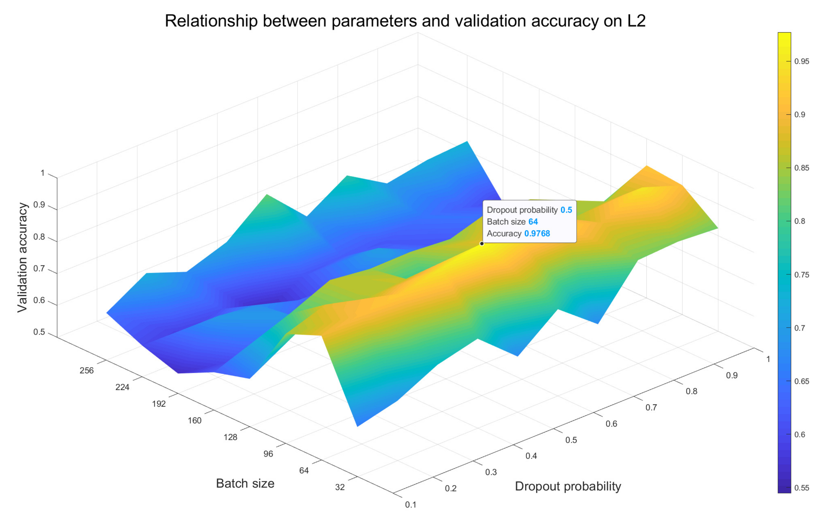
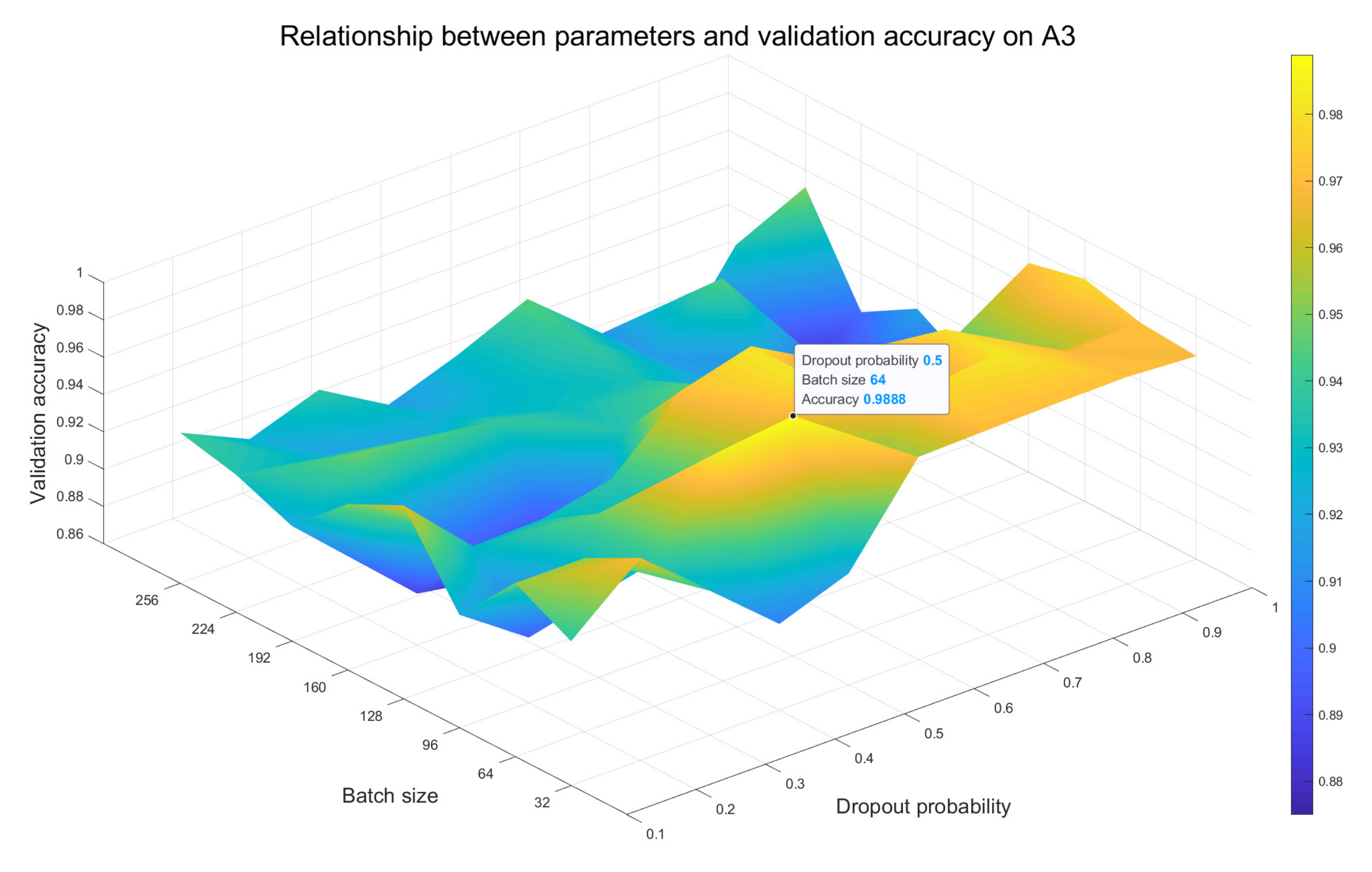
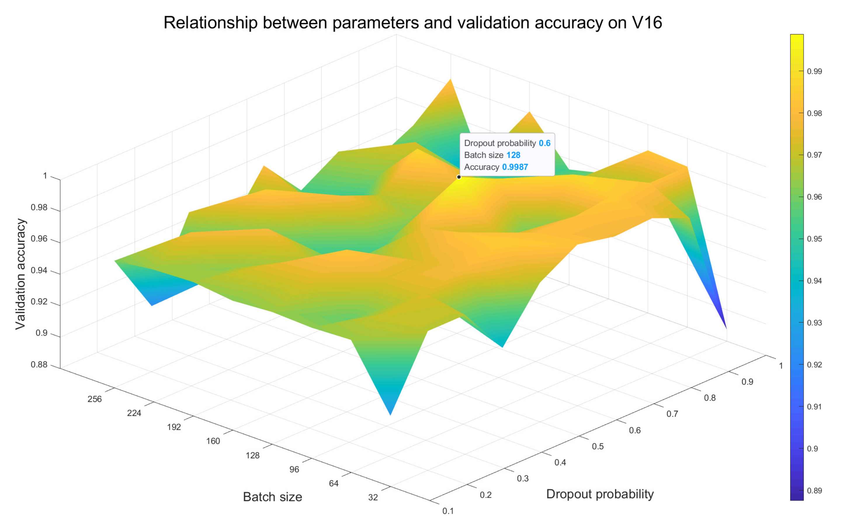
• Dropout [32]: by randomly removing the nodes of the network during the training process, a single model can simulate a large number of different architectures, which is called the dropout method. It provides a very low computational cost and very effective regularization approach to alleviate overfitting of deep neural networks and improve the generalization performance. When this method is used in our experiments, we add a dropout layer to each fully connected layer, which reduces the interdependence between the neuron nodes in the network by deactivating some neurons with a certain probability value (making the output of the neurons zero). In our experiment, we train models by jointly adjusting the probability value of the dropout layer and the batch size value. First, we try to set the probability value of dropout layers to the value in (0.1, 0.2, 0.3, 0.4, 0.5, 0.6, 0.7, 0.8, 0.9, 1). Second, through multiple experiments, we select the best combination of dropout and batch size values.
• Shuffle: to eliminate the potential impact of the order in which the training data are fed into the network and further increase the randomness of the training data samples, we introduce the shuffle method into the model evaluation experiments. Specifically, when this method is applied, we shuffle all training samples in each new training epoch, and then input each shuffled data batch into the network.

3. Results

To find models with stable performance and high OBI character recognition accuracy among the ten proposed CNN models, we conducted the following three kinds of experiments and observed each set of experimental results.

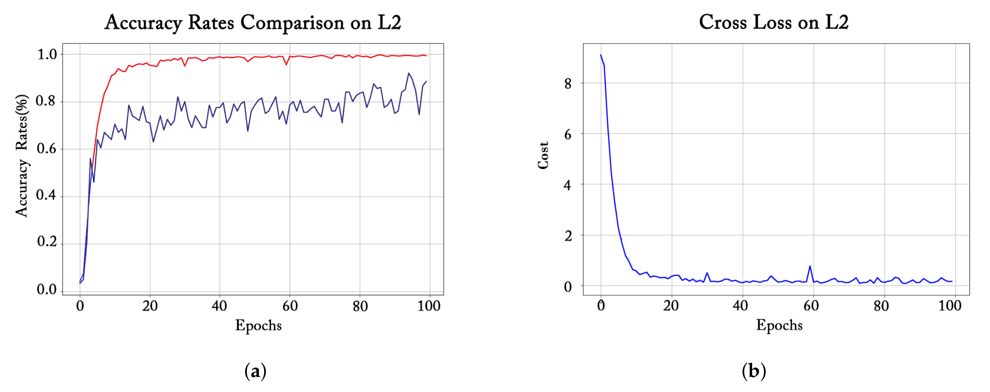
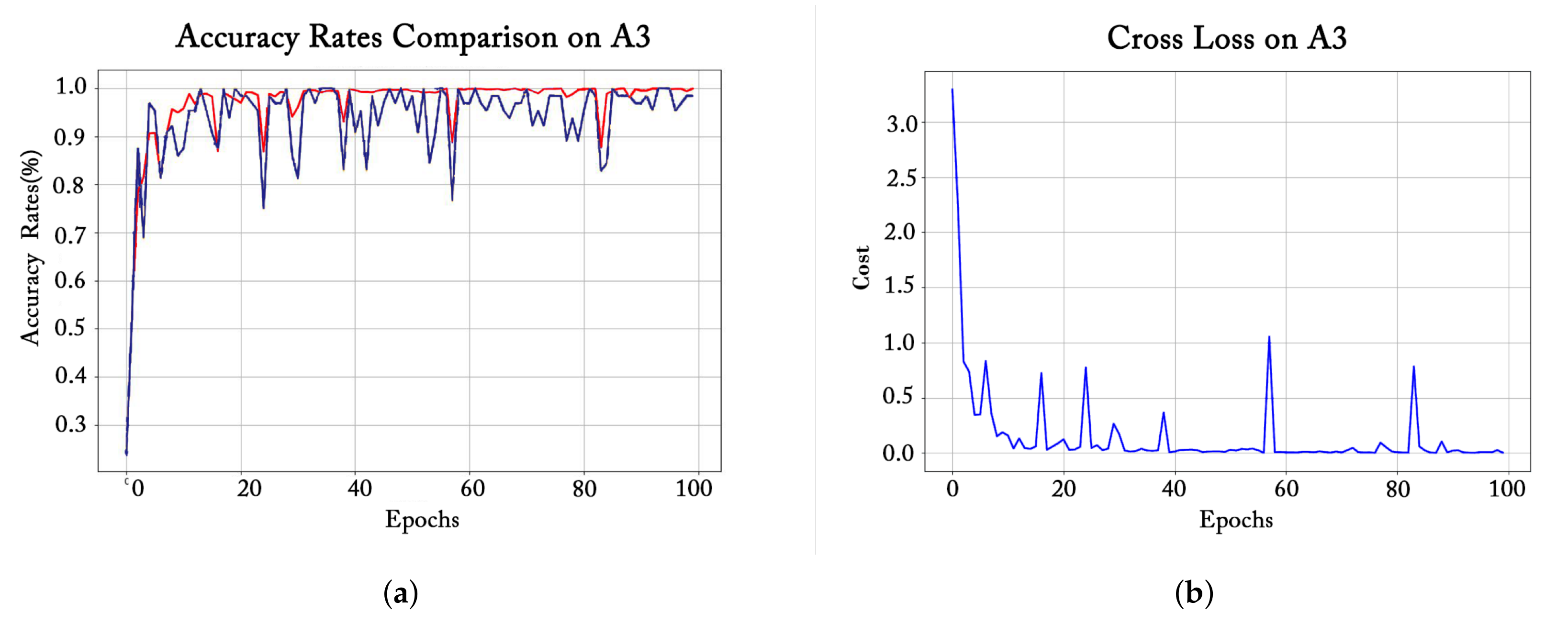
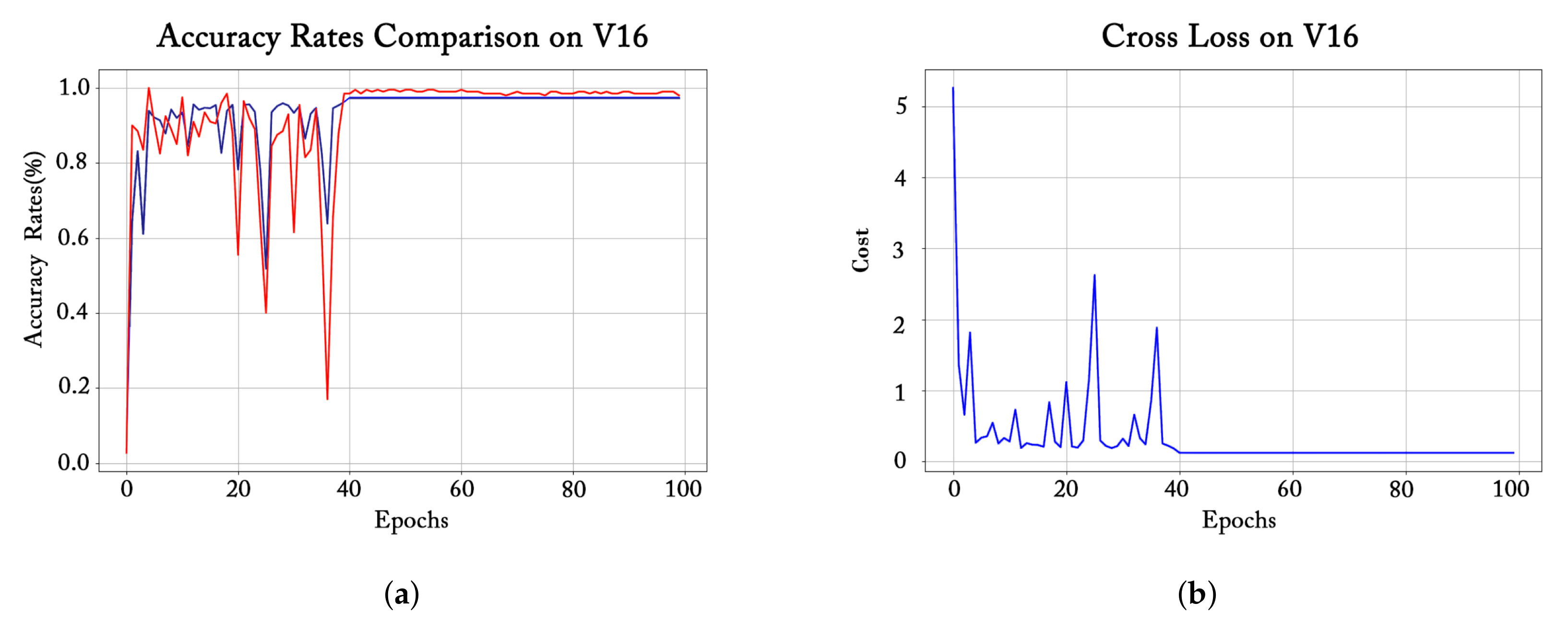
• We visualized the changes in the training loss value, the accuracy rates on the training set and the validation set of different models during the training process as the number of training epochs increases. In addition, by comparing the training accuracy and validation accuracy, we can infer the overall learning effect of the models corresponding to each epoch. These are discussed in Section 3.1.
• For different models, we test the impact of multiple combinations of batch size value and dropout probability value on recognition accuracy of the validation set. By comparison, the optimal combination of these two parameters is selected as the setting strategy for the final performance experiment of the corresponding model. The results are mainly analyzed in Section 3.2.
• From the three aspects of data augmentation, model structure adjustment, and optimization implementation, we evaluate the effects of various improvement methods on model learning and OBI recognition. Results and discussions are presented in Section 3.3.

3.1. Training Process Observation

For the three groups of improved models corresponding to the three basic CNN frameworks, we chose one from each group to observe the corresponding training process, as shown in Figure 8, Figure 9 and Figure 10. For each left graph, the blue line represents the validation accuracy (recognition accuracy on the validation set), and the red line refers to the training accuracy (recognition accuracy on the training set). Each figure on the right shows the relationship between training loss and training epochs.

Figure 8. Training accuracy, validation accuracy, and training loss during L2 model training. (a) Accuracy comparison. (b) Cross loss.

Figure 9. Training accuracy, validation accuracy and training loss during A3 model training. (a) Accuracy comparison. (b) Cross loss.

Figure 10. Training accuracy, validation accuracy, and training loss during V16 model training. (a) Accuracy comparison. (b) Cross loss.

The training process of the L2 model (one of the improved LeNet models) is shown in Figure 8. We can see that, in the first 10 epochs of training, the training loss value drops sharply and the training accuracy rises dramatically, indicating that the model is learning effectively. From the 10th epoch to the 40th epoch, the training loss still shows a downward trend until it stabilizes after 40 epochs, which is also consistent with the change in training accuracy. However, although the validation accuracy rate is also on the rise, when approaching 100 epochs, the training set accuracy rate is close to 1, while the accuracy rate on the validation set is lower than 90% and continues to fluctuate, which demonstrates that only training for 100 epochs cannot make the L2 model fully converge.

For the A3 model (one of the improved AlexNet models) in Figure 9, the accuracy rates on the training set and the validation set basically maintain a consistent trend on the whole. Specifically, in the first ten epochs of training, both curves rise rapidly. After 10 epochs, the training accuracy gradually tends to 100% and becomes smooth, while the validation accuracy curve still has large fluctuations. This suggests that the learning of the A3 model is not stable enough despite the high recognition accuracy within 100 epochs.

The training process of the V16 model (one of the improved VGGNet models) is shown in Figure 10. From these two graphs, we can clearly observe that on the V16 model, both the training and validation accuracy rates increase with very sharp fluctuations in the first 40 epochs, and these fluctuations also occur on the training loss curve. However, after the 40th epoch, the training and validation accuracy curves are smoothed around 100%, and the training accuracy is slightly higher than the validation accuracy. From this we conclude that the V16 model only needs about 40 epochs to converge and has good recognition performance.

3.2. Parameter Effect Evaluation

We keep the other hyperparameters of the network unchanged and adjust the values of batch size and dropout probability associatively to observe the recognition accuracy on the validation set of the model, where the value of batch size is taken from (32, 64, 96, 128, 160, 192, 224, 256) and that of dropout probability is taken from (0.1, 0.2, 0.3, 0.4, 0.5, 0.6, 0.7, 0.8, 0.9, 1). Surface plots of the relationship between batch size, dropout probability and validation accuracy rate on L2, A3 and V16 models are obtained as Figure 11, Figure 12 and Figure 13, respectively. We use a black dot to mark the point with the highest accuracy on each surface, and mark the corresponding x and y coordinates next to that point.

Figure 11. Surface plot on the L2 model displaying the resulting validation recognition accuracy for different choices of values of the batch size and the dropout probability.

Figure 12. Surface plot on the A3 model displaying the resulting validation recognition accuracy for different choices of values of the batch size and the dropout probability.

Figure 13. Surface plot on the V16 model displaying the resulting validation recognition accuracy for different choices of values of the batch size and the dropout probability.

According to the color change of the surface plots, it can be inferred that the more drastic the color system changes, the greater the impact of different choices of values of the batch size and the dropout probability on the models is. From Figure 11 we see that there are obvious blue and yellow areas, indicating that the accuracy of the L2 model is most affected by these two parameters, followed by the A3 model in Figure 12. The color system of the surface map in Figure 13 corresponding to the V16 model changes smoothly, so it is minimally affected by the two parameters. In addition, the highest point indicates the optimal combination of batch size and dropout probability values. For the L2 and A3 models, setting the batch size and dropout probability values to 64 and 0.5 is the optimal choice, while for the V16 model, they should be set to 128 and 0.6, respectively.

3.3. Model Performance Overview

From the above experimental results, we obtain the best combination of batch size and dropout probability values used to train each model. In the next experiment, we use the optimization methods mentioned in Section 2.3.3 and the optimal hyperparameter combination configurations to train the classical and the proposed improved models. In addition, to evaluate the effect of data augmentation for the OBI-100 dataset, these models are also trained and tested on the non-augmented dataset. A general overview of the final results is shown in Table 2, Table 3 and Table 4.

Table 2. Recognition accuracy of LeNet-based models on unaugmented (No) and augmented (Yes) OBI datasets. BN, DP, SF represent batch normalization, dropout, and shuffle methods, respectively. Test (max) denotes the maximum recognition accuracy rate and Test (ave) represents the average value of the last five accuracy rates after the training is stable. Bold numbers indicate the optimal value of each indicator in each group of network frameworks.

Model	Data Augment	Method	Accuracy (%)
			Test (Max)	Test (Ave)
Based on LeNet
LeNet	No	-	71.23	-
L1		SF	78.77	78.77
L2		SF	74.20	-
LeNet	Yes	-	81.25	75.00
		SF + BN + DP	85.41	82.37
L1		SF	95.35	92.48
		SF + BN	97.15	96.56
		SF + BN + DP	98.43	97.93
L2		SF	93.75	87.50
		SF + BN	94.25	88.80
		SF + BN + DP	96.88	86.93

Table 3. Recognition accuracy of AlexNet-based models on unaugmented (No) and augmented (Yes) OBI datasets. BN, DP, SF represent batch normalization, dropout, and shuffle methods, respectively. Test (max) denotes the maximum recognition accuracy rate and Test (ave) represents the average value of the last five accuracy rates after the training is stable. Bold numbers indicate the optimal value of each indicator in each group of network frameworks.

Model	Data Augment	Method	Accuracy (%)
			Test (Max)	Test (Ave)
Based on AlexNet
AlexNet	No	-	71.23	-
A1		DP	84.47	-
A2		DP + SF	89.80	-
A3		DP + SF	91.32	-
AlexNet	Yes	-	79.40	76.91
		DP + SF + BN	91.66	89.97
A1		DP	92.19	92.17
		DP + SF	94.12	93.11
		DP + SF + BN	96.75	94.05
A2		DP + SF	96.88	91.04
		DP + SF + BN	97.05	93.76
A3		DP + SF	98.44	93.25
		DP + SF + BN	98.48	95.38

Table 4. Recognition accuracy of VGGNet-based models on unaugmented (No) and augmented (Yes) OBI datasets. VGG n refers to the standard VGGNet model with a n-layer structure. BN, DP, SF represent batch normalization, dropout, and shuffle methods, respectively. Test (max) denotes the maximum recognition accuracy rate and test (ave) represents the average value of the last five accuracy rates after the training is stable. Bold numbers indicate the optimal value of each indicator in each group of network frameworks.

Model	Data Augment	Method	Accuracy (%)
			Test (Max)	Test (Ave)
Based on VGGNet
VGG11	No	-	84.88	-
V11		BN	85.56	-
VGG13		-	85.03	-
V13		BN + SF	85.10	-
VGG16		-	93.75	-
V16		BN + SF	91.28	-
VGG19		-	90.35	-
V19		BN + SF	89.71	-
Based on VGGNet
VGG11	Yes	-	91.10	90.39
		BN + SF + DP	92.96	92.18
V11		BN	91.20	91.10
		BN + SF	91.80	91.20
		BN + SF + DP	94.66	92.50
VGG13		-	92.88	90.67
		BN + SF + DP	94.31	93.21
V13		BN + SF	93.20	91.75
		BN + SF + DP	95.85	95.10
VGG16		-	96.24	93.75
		BN + SF + DP	97.75	95.65
V16		BN + SF	99.49	99.00
		BN + SF + DP	99.50	99.50
V16-2		BN + SF	95.30	94.13
		BN + SF + DP	95.60	94.38
VGG19		-	96.67	96.28
		BN + SF + DP	98.26	97.75
V19		BN + SF	98.40	98.20
		BN + SF + DP	98.75	98.61

From Table 2, Table 3 and Table 4, on the one hand, we can simply observe that the data augmentation strategy can generally enhance the recognition accuracy of the models. For example, the L1 model trained on the shuffled unaugmented training set gets a maximum accuracy of only 78.77% for the simpler unaugmented test set classification task, while the L1 model learned on the augmented OBI-100 yields an accuracy of 95.35% against the more difficult augmented sample recognition task. On the other hand, we notice that compared with the original models of the three classic frameworks, the improved networks show better recognition performance on the augmented OBI dataset. Specifically, when integrating the three optimization methods, the L1 and L2 models achieve 13.02% and 11.47% higher recognition performance than the original LeNet respectively, while the A1, A2, and A3 models yield 5.09%, 5.39%, and 6.82% improvement in recognition accuracy respectively, compared to the original AlexNet. In addition, the performance baseline of the original VGGNet-based models is relatively high, but the improved model still results in performance gains. For instance, the accuracy of the optimal V16 model is 99.50%, while the original VGG16 model only achieves 97.75%.

Moreover, adding suitable optimization methods contributes a lot to the recognition accuracy of the models. For instance, for the V11 model trained on the augmented OBI-100, the maximum test accuracy reaches 91.20% when using batch normalization only, and the accuracy is enhanced to 91.80% after using shuffle optimization, and it is further improved to 94.66% after applying the dropout method. Similar accuracy improvements can be clearly observed in the experimental results of each proposed model.

For each group of enhanced models, we also make the following observations. Firstly, the LeNet-based L1 model is significantly better than the L2 model. On the one hand, the best maximum test accuracy of the L1 model is higher than that of the L2 model, and on the other hand, the gap between the maximum test rate and the average test rate of the L1 model is a smaller value of 0.5%, indicating that the training effect of the L1 model is more stable.

Thirdly, from Table 4, one can see that the increase in the number of network layers has a beneficial effect on the recognition performance of the VGGNet-based models. Specifically, V11, V13, and V16 with the same fully connected layer structures, respectively, get the best accuracy rates of 94.66%, 95.85%, and 99.50%, incrementally. In addition, for V16 and V16-2 with the same network structures of convolutional and pooling layers, the V16 model with deeper fully connected layers outperforms the V16-2 model by 3.9%. We also observe that the maximum accuracy on the V16 model is the same as the average accuracy, indicating that the V16 model performs more effective feature learning on the OBI-100 dataset.

Finally, from Table 2, Table 3 and Table 4, it is obtained that the VGGNet-based V16 model, for one, achieves the highest accuracy of 99.5% on the OBI-100 dataset, for another, the maximum and average accuracy values of this model are the same, so it is the best model for identifying the OBI-100 dataset in our experiments.

4. Conclusions

In this work, deep convolutional neural networks are used to identify oracle characters. We created a standardized dataset called OBI-100, which contains 100 classes of characters of OBI. OBI-100 can fill the gap of publicly available datasets in the applications of deep learning in OBI research. Base on three typical convolutional network frameworks, ten improved models are proposed to classify the characters of OBI. Through a large number of experiments and a variety of optimization methods, the best model achieves an accuracy of 99.5% in the 100-class OBI recognition task. Our work shows that characters of OBI can be recognized practically and effectively in deep convolutional neural networks, and applications in this area have broad research prospects, which also provide new ideas for studying the origin of words and human history.

References

- Keightley, D.N. The Shang State as Seen in the Oracle-Bone Inscriptions. Early China 1980, 5, 25–34. [Google Scholar] [CrossRef]
- Flad, R.K. Divination and Power: A Multiregional View of the Development of Oracle Bone Divination in Early China. Curr. Anthropol. 2008, 49, 403–437. [Google Scholar] [CrossRef] [Green Version]
- Guo, J.; Wang, C.; Rangel, E.R.; Chao, H.; Rui, Y. Building Hierarchical Representations for Oracle Character and Sketch Recognition. IEEE Trans. Image Process. 2015, 25, 104–118. [Google Scholar] [CrossRef] [PubMed]
- Keightley, D.N. Graphs, Words, and Meanings: Three Reference Works for Shang Oracle-Bone Studies, with an Excursus on the Religious Role of the Day or Sun. J. Am. Orient. Soc. 1997, 117, 507–524. [Google Scholar] [CrossRef]
- Bazerman, C. Handbook of research on writing: History, society, school, individual, text. Delta Doc. Estud. Lingüística Teórica E Apl. 2008, 24, 419–420. [Google Scholar]
- Dress, A.; Grünewald, S.; Zeng, Z. A cognitive network for oracle bone characters related to animals. Int. J. Mod. Phys. B 2016, 30, 1630001. [Google Scholar] [CrossRef]
- Feng, Y. Recognition of jia gu wen based on graph theory. J. Electron. Inf. Technol. 1996, 18, 41–47. [Google Scholar]
- Li, Q.; Wu, Q.; Yang, Y. Dynamic Description Library for Jiaguwen Characters and the Reserch of the Characters Processing. Acta Sci. Nat. Univ. Pekin. 2013, 49, 61–67. [Google Scholar]
- Lu, X.; Li, M.; Cai, K.; Wang, X.; Tang, Y. A graphic-based method for Chinese Oracle-bone classification. J. Beijing Inf. Sci. Technol. Univ. 2010, 25, 92–96. [Google Scholar]
- Gu, S. Identification of Oracle-bone Script Fonts Based on Topological Registration. Comput. Digit. Eng. 2016, 44, 2001–2006. [Google Scholar]
- Meng, L. Two-Stage Recognition for Oracle Bone Inscriptions. In Proceedings of the ICIAP, Catania, Italy, 11–15 September 2017. [Google Scholar]
- Meng, L. Recognition of Oracle Bone Inscriptions by Extracting Line Features on Image Processing. In Proceedings of the ICPRAM, Porto, Portugal, 24–26 February 2017. [Google Scholar]
- Liu, Y.; Liu, G. Oracle character recognition based on SVM. J. Anyang Norm. Univ. 2017, 2, 54–56. [Google Scholar]
- Gjorgjevikj, D.; Cakmakov, D. Handwritten Digit Recognition by Combining SVM Classifiers. In Proceedings of the Eurocon 2005—The International Conference on “computer as a Tool”, Belgrade, Serbia, 21–24 November 2005. [Google Scholar]
- Gao, F.; Xiong, J.; Liu, Y. Recognition of Fuzzy Characters on Oracle-Bone Inscriptions. In Proceedings of the IEEE International Conference on Computer & Information Technology; Ubiquitous Computing & Communications; Dependable, Autonomic and Secure Computing; Pervasive Intelligence and Computing, Liverpool, UK, 26–28 October 2015. [Google Scholar]
- Institute of Archaeology, Chinese Academy of Sciences. Oracle Bone Inscriptions Collection; Zhonghua Book Company: Beijing, China, 1965. [Google Scholar]
- Wang, B. 100 Cases of Classical Oracle Bone Inscription Rubbings; Beijing Arts and Crafts Publishing House: Beijing, China, 2015. [Google Scholar]
- Froment, J. Parameter-Free Fast Pixelwise Non-Local Means Denoising. Image Process. Line 2014, 4, 300–326. [Google Scholar] [CrossRef] [Green Version]
- Buades, A.; Coll, B.; Morel, J.M. Non-Local Means Denoising. Image Process. Line 2011, 1, 208–212. [Google Scholar] [CrossRef] [Green Version]
- Chen, S.; Haralick, R.M. Recursive Erosion, Dilation, Opening, and Closing Transforms. IEEE Trans. Image Process. 1995, 4, 335–345. [Google Scholar] [CrossRef] [PubMed]
- Kim, P. Convolutional Neural Network In MATLAB Deep Learning: With Machine Learning, Neural Networks and Artificial Intelligence; Apress: Berkeley, CA, USA, 2017. [Google Scholar]
- Maitra, D.S.; Bhattacharya, U.; Parui, S.K. CNN based common approach to handwritten character recognition of multiple scripts. In Proceedings of the 2015 13th International Conference on Document Analysis and Recognition (ICDAR), Tunis, Tunisia, 23–26 August 2015. [Google Scholar]
- Heaton, J. Deep learning. Genet. Program. Evolvable Mach. 2018, 19, 305–307. [Google Scholar] [CrossRef] [Green Version]
- Hinton, G.E.; Osindero, S.; Teh, Y.W. A Fast Learning Algorithm for Deep Belief Nets. Neural Comput. 2006, 18, 1527–1554. [Google Scholar] [CrossRef] [PubMed]
- Krizhevsky, A.; Sutskever, I.; Hinton, G.E. ImageNet Classification with Deep Convolutional Neural Networks. In Proceedings of the International Conference on Neural Information Processing Systems, Lake Tahoe, NV, USA, 3–6 December 2012. [Google Scholar]
- Zhou, B.; Lapedriza, A.; Xiao, J.; Torralba, A.; Oliva, A. Learning Deep Features for Scene Recognition using Places Database. Adv. Neural Inf. Process. Syst. 2015, 1, 487–495. [Google Scholar]
- Bishop, C.M. Neural Networks for Pattern Recognition. Agric. Eng. Int. Cigr J. Sci. Res. Dev. Manuscr. Pm 1995, 12, 1235–1242. [Google Scholar]
- Le Cun, Y.; Jackel, L.D.; Boser, B.; Denker, J.S.; Graf, H.P.; Guyon, I.; Henderson, D.; Howard, R.E.; Hubbard, W. Handwritten Digit Recognition: Applications of Neural Net Chips and Automatic Learning. IEEE Commun. Mag. 1989, 27, 41–46. [Google Scholar] [CrossRef]
- Simonyan, K.; Zisserman, A. VVery Deep Convolutional Networks for Large-Scale Image Recognition. In Proceedings of the 3rd International Conference on Learning Representations, ICLR 2015, San Diego, CA, USA, 7–9 May 2015. [Google Scholar]
- He, K.; Zhang, X.; Ren, S.; Sun, J. Delving Deep into Rectifiers: Surpassing Human-Level Performance on ImageNet Classification. In Proceedings of the ICCV, Santiago, Chile, 7–13 December 2015. [Google Scholar]
- Ioffe, S.; Szegedy, C. Batch normalization: Accelerating deep network training by reducing internal covariate shift. In Proceedings of the International Conference on Machine Learning, Lille, France, 7–9 July 2015. [Google Scholar]
- Srivastava, N.; Hinton, G.; Krizhevsky, A.; Sutskever, I.; Salakhutdinov, R. Dropout: A Simple Way to Prevent Neural Networks from Overfitting. J. Mach. Learn. Res. 2014, 15, 1929–1958. [Google Scholar]