Deep Descriptor Learning with Auxiliary Classification Loss for Retrieving Images of Silk Fabrics in the Context of Preserving European Silk Heritage

Abstract

With the growing number of digitally available collections consisting of images depicting relevant objects from the past in relation with descriptive annotations, the need for suitable information retrieval techniques is becoming increasingly important to support historians in their work. In this context, we address the problem of image retrieval for searching records in a database of silk fabrics. The descriptors, used as an index to the database, are learned by a convolutional neural network, exploiting the available annotations to automatically generate training data. Descriptor learning is combined with auxiliary classification loss with the aim of supporting the clustering in the descriptor space with respect to the properties of the depicted silk objects, such as the place or time of origin. We evaluate our approach on a dataset of fabric images in a kNN-classification, showing promising results with respect to the ability of the descriptors to represent semantic properties of silk fabrics; integrating the auxiliary loss improves the overall accuracy by 2.7% and the average F1 score by 5.6%. It can be observed that the largest improvements can be obtained for variables with imbalanced class distributions. An evaluation on the WikiArt dataset demonstrates the transferability of our approach to other digital collections.

1. Introduction

Preserving our cultural heritage for future generations and making it available to both historians and a wider public is an important task. In this context, a key strategy is the digitization of collections of historical objects in the form of searchable databases with standardized annotations and, potentially, images, which is also a prerequisite for fast and easy access to the related knowledge by both expert and non-expert users. It was the goal of the EU H2020 project SILKNOW (http://silknow.eu/, visited on 30 November 2021) to take one step in this direction for the preservation of European cultural heritage related to silk. Silk has played an important role in many different areas for hundreds of years and still does so in the present. For instance, it has triggered technical developments such as the Jacquard loom, which introduced the concept of punched cards for storing information. It also has an economic impact through the textile and creative industries and a functional aspect as a component of clothes and furniture, and it is also relevant from a cultural and symbolic perspective through forming individuality and identity [1]. To make silk-related knowledge from the past accessible for future generations, a knowledge graph related to silk fabrics was built by harvesting existing online collections and converting the meta-information into a standardized format [1]. The present paper is motivated by the requirement to provide easy access to this knowledge graph and presents a new deep learning-based method for image retrieval that can be used to search for records in a database on the basis of images.

For image retrieval, a feature vector (descriptor) is pre-computed for every image available in the database. As soon as a user provides a query image, a corresponding query descriptor is derived, which serves as an index to the database: the images that are most similar to the query image are identified by finding the most similar descriptors of database images, typically using the Euclidean distance as a similarity measure. To speed up the search for nearest neighbors, the descriptors of the images from the database are stored in a spatial index, typically a kd-tree [2]. Several approaches for image retrieval have focused on hand-crafted image descriptors; e.g., encoding visual properties of images [3,4] or exploiting text associated with images [5]. More recent approaches utilize methods based on convolutional neural networks (CNNs) [6,7] to learn descriptors that reflect the similarity of image pairs. The training process of such a CNN usually requires training samples consisting of pairs of images with a known similarity status; i.e., it has to be known whether the two images of a training pair are similar or dissimilar [8]. In the training process, the network learns to generate descriptors with small Euclidean distances for similar image pairs and descriptors with large Euclidean distances for dissimilar ones.

In this context, a major problem is the generation of training samples. Often, they are generated by manual labeling [9,10], but this is a tedious and time-consuming task; in the context of image retrieval for searching in a database of works of art, it also has the disadvantage that, in particular if based on purely visual aspects, it is highly subjective. To solve this problem, it is desirable to generate the training samples automatically by defining similarity based on additional information that is assigned to images; e.g., class labels describing the type of the depicted object [11,12,13,14] or descriptive texts [15,16]. This strategy for generating training data was also applied for image retrieval in the context of digital collections of works of art [17,18,19]. It allows the generation of samples consisting of pairs of images with a known similarity status from existing datasets containing images with annotations. In most of the cited approaches, the similarity of images is considered to be a binary concept: a pair of images is either similar or not [11,17].

However, in the context of image retrieval in databases of works of art, a gradual concept of similarity [13,14] might be more intuitive than a binary one. One option to define such a non-binary concept of similarity can be obtained by measuring the level of similarity of an image pair by the level of agreement of the semantic annotations for multiple variables—a concept we referred to as semantic similarity in [20,21]. In these works, we also considered the problem of missing information: if harvested automatically from online collections of museums, many records in a database containing information about cultural heritage objects will not contain annotations for all variables considered to be relevant for defining similarity.

In this paper, we present a CNN-based method for image retrieval that can be applied to any database containing images with semantic annotations. Based on our previous work [21], training samples are determined automatically from the database, leading to a gradual concept of semantic similarity, which also can be combined with visual ones. This is expected to lead to retrieval results that are particularly meaningful for persons wanting to learn something about the properties of the query images by analyzing the annotations of the retrieved images, and it also allows a quantitative evaluation based on a k-nearest neighbor (kNN) classification. Our method also allows for samples with incomplete annotations to be considered in training. Compared to our previous work, we modify the training loss for learning similarity slightly and, more importantly, add an additional auxiliary classification loss for every training sample, which we expect to support the clustering in the descriptor space by forcing the descriptors to have a better intra-class connectivity.

The scientific contributions of this paper can be formulated as follows:

• To the best of our knowledge, ours is the first work exploiting class labels of multiple semantic variables for defining similarity for image retrieval in combination with in an auxiliary classification loss in an end-to-end training strategy. Existing works employing an auxiliary classification loss that we are aware of [22,23,24] do not exploit multiple variables and thus do not use a gradual concept of similarity.
• We use a gradual rather than a binary concept of similarity of images based on multiple semantic variables while taking into account the problem of missing annotations, which is important when dealing with collections of records harvested from the internet. Other works implicitly allow a different number of labels per image because the scene contains multiple objects, e.g., [12,13,14], which is not the case in our application.
• We transfer the gradual definition of the similarity status of image pairs into the triplet loss of [25] to learn fine-grained image representations so that the Euclidean distances of the learned descriptors are forced to reflect the different degrees of similarity without the need to carefully select a margin in the loss. The margin is adapted to the degree of similarity and uncertainty of the similarity status.
• Our formulation of the loss allows us to combine different concepts of similarity for training to obtain descriptors that are both visually as well as semantically similar.
• We present an extensive set of experiments based on a dataset of silk fabrics, using kNN classification for a quantitative evaluation, which also highlights the impact of the classification loss on the results. To show the transferability of the approach, we also present experiments for image retrieval based on the WikiArt dataset (http://www.wikiart.org, visited on 30 November 2021).

The remainder of this paper starts with an overview about the related work (Section 2). Our new method for image retrieval is presented in Section 3. Section 4 describes the datasets used for the evaluation of this method, whereas Section 5 presents a comprehensive set of experiments based on these datasets. Finally, Section 6 summarizes our main findings and makes suggestions for future work.

2. Related Work

Early work on image retrieval relied on hand-crafted features. In content-based image retrieval (CBIR), the descriptors exclusively reflect the visual content of an image in form of color histogram features, shape features and texture features [3,4]. As such, these features focus on the visual appearance of images, and the retrieval results are often not representative on a conceptual level, which is referred to as the semantic gap [26]. In order to provide semantically meaningful retrieval results and thus to overcome this semantic gap, additional semantic features derived from textual annotations of images have been investigated in the context of semantic-based image retrieval (SBIR). For instance, ref. [27] derived text features from image captions among others that can be integrated in image retrieval [5]. However, none of these early works learn the descriptors from training data, which is considered to be the strength of methods based on deep learning.

It was already shown in [28] that representations derived by a CNN pre-trained for a completely different task, e.g., classification, can be used to achieve more meaningful image retrieval results than classical methods specifically designed for image retrieval. Many deep learning approaches designed for image retrieval apply Siamese CNNs consisting of two branches with shared weights [29]. When training a Siamese network, the contrastive loss [8] is often applied. It forces the network to produce similar descriptors for image pairs considered to be similar and to produce dissimilar descriptors for image pairs considered to be dissimilar. As the Euclidean distance is used to measure the similarity of descriptors in this loss, it can also be used for image retrieval, e.g., [10]. Whereas training with a contrastive loss requires pairs of images that are either similar or dissimilar, the triplet loss [9] requires image triplets, each consisting of an anchor image, a positive sample—i.e., an image defined to be similar to the anchor—and a negative sample that is dissimilar to the anchor. This loss forces the descriptor of the positive sample to be more similar to the descriptor of the anchor in terms of the Euclidean distance than the descriptor of the negative sample by at least a predefined margin. Both training procedures require training samples with known binary similarity status, which are often generated by manual labeling; e.g., [9,10].

2.1. Exploiting Semantic Annotations

An alternative to manual labeling is to exploit semantic annotations assigned to the images to define similarity. A straightforward way to do this while maintaining a binary similarity concept is to consider class labels of one semantic variable only: if two images have the same class label, they are considered to be similar; otherwise, they are dissimilar. An example for such an approach is [11], where the resultant pairs with a known binary similarity status are used in a training procedure involving the triplet loss. Although this strategy solves the problem of manual labeling if a database with annotated images is available, the similarity status of an image pair is still defined in a binary way, which does not take into account the fact that some images may be considered more similar to each other than others and does not allow a method to be trained to retrieve images that are similar to the query image with respect to multiple semantic variables.

If multiple annotations per image are considered, different degrees of similarity of two images can be defined [12,13,14]. In [12], different levels of semantic similarity are defined on the basis of the number of identical labels assigned to two images. Training is based on a triplet loss, using the different degrees of similarity to weight the importance of a triplet in training while maintaining a constant margin hyperparameter. Thus, the minimal distance that is enforced between the distances of the descriptors of the positive and the negative samples from the anchor descriptor is identical for all triplets, independently of their degree of similarity.

In [13], training requires the descriptor distances to reflect different degrees of similarity. Using the contrastive loss, descriptors of images whose annotations agree completely are forced to have a distance shorter than a pre-defined positive margin, whereas the margin defining the minimal descriptor distance between images with partly or completely different annotations is weighted by the degree of similarity; the margin is a hyperparameter to be chosen. A gradual definition of semantic similarity based on the cosine distance between two label vectors is proposed in [14]. The authors formulate a loss based on pairs of images that forces the image descriptor similarity to match the gradual semantic similarity during training without the need to tune a margin hyperparameter.

All of the cited papers using multiple annotations [12,13,14] aim to learn binary hash codes as image descriptors instead of real-valued feature vectors. The labels used in these papers describe different aspects of the depicted scene, e.g., different object types, whereas in our work, they are related to more abstract semantic properties of the depicted object, e.g., the place and time of origin of the depicted object. Furthermore, even though they allow for a different number of labels assigned to an image, the cited papers do not consider missing annotations in theirs definitions of similarity. We explicitly deal with missing annotations in triplet-based learning, using them to define a degree of uncertainty of the similarity status that has an impact on the margin of the triplet loss.

2.2. Auxiliary Losses

The usability of feature vectors learned in the context of image classification to serve as descriptors for image retrieval has already been investigated [28,30,31,32]. Even leveraging the softmax layer activations for image retrieval seems to be possible [33]. In [34], classification is used to restrict the search space for image retrieval to the images belonging to the same category as the search image. To further improve the clustering of image descriptors with respect to the similarity of the represented images, descriptor learning can be realized by combining the pairwise or triplet losses with an additional auxiliary classification loss.

In [22], descriptor learning based on the contrastive loss is combined with a classification loss. A single variable only is considered both for defining the similarity of images in a binary way and for classification. Similar approaches relying on a single variable are shown in [23,24], but in these papers, the triplet loss is used in combination with a classification loss. This is also the case in [35], where two additional auxiliary loss functions are proposed: a spherical loss, designed to support the learning of inter-class separability, and a center loss, expected to support the intra-class connectivity. All of these works exploit the class labels of one variable only to define similarity, which leads to a binary similarity status of images and thus does not allow different degrees of similarity to be learned. In [36], descriptor learning is also combined with a classification loss, where several semantic variables are used to perform multi-task learning. The goal of descriptor learning is to force the high-level image descriptors that are produced by the last layer of the feature extractor to be invariant to the characteristics of the dataset an image belongs to; in [36], two different descriptors are considered. For that purpose, the descriptors produced by two multi-task network architectures, one per dataset, are presented to a triplet loss, forcing the descriptors belonging to different datasets to be more similar than a descriptor pair belonging to images from the same dataset. Although [36] exploits the class labels of several variables to learn descriptors by means of multi-task learning, the concept of similarity is still defined in a binary way.

We could identify exactly one work that allows for a fine-grained definition of similarity and additionally utilizes a classification loss to support descriptor learning. In [37], a fine-grained definition of similarity by exploiting the semantic relatedness of class labels according to their relative distance in a WordNet ontology [38] is proposed. Descriptor training, which can be optionally combined with the training of a classifier, is realized by learning a mapping from images to embeddings that are enforced to match pre-calculated class embeddings, where the class embeddings can iteratively be derived from a similarity measure for images considering semantic aspects. To the best of our knowledge, there is no work that learns different degrees of descriptor similarity in combination with a classification loss in an end-to-end manner. In particular, we could not find any work that exploits the classes of several semantic variables to both define a fine-grained concept of semantic similarity and to learn to predict the variables in order to support descriptor learning.

2.3. Image Retrieval for Cultural Heritage

All works cited so far address descriptor learning for image retrieval, but in the context of applications that do not involve the preservation of cultural heritage. Many works investigating machine learning methods in the field of heritage preservation focus on the image-based classification of depicted artworks with respect to one [39,40,41] or multiple variables [42,43,44]. Nevertheless, image retrieval is becoming an increasingly important task in that field as well [45].

The first approaches exploit graph-based representations of images in order to search for similar objects in a database [46]. More recent approaches for image retrieval in the context of cultural heritage rely on high-level image features learned by a CNN; e.g., [17,47]. In [47], an unsupervised approach for image retrieval based on extracting image features with a pre-trained CNN is proposed. After transforming these features to more compact descriptors by means of a principal component analysis, image retrieval is performed by searching the nearest neighbors in the descriptor space based on Euclidean distances. In contrast, the authors of [17] propose to train a CNN to generate image features suitable for retrieval by minimizing a triplet loss. For that purpose, they generate training data exploiting the class labels of five semantic variables to define the similarity of images in a binary way; two images are assumed to be similar in cases with more than two identical class labels.

Instead of aiming to retrieve the images that are most similar to a query image, cross-modal retrieval aims at finding the images most closely related to a provided query text or at finding the best descriptive texts for a query image. Cross-modal image retrieval plays an important role in the context of querying art collections, e.g., [18,19], where it is a challenging task to match images and texts in cultural heritage related collections [48]. In [18], descriptors are learned by minimizing a variant of the triplet loss, where image descriptors and text descriptors are forced to be similar with respect to their dot product. The approach in [19] also addresses cross-modal retrieval using strategies that are similar to the ones used in our work. The authors obtain image descriptors for retrieval on the basis of a CNN (ContextNet) pre-trained for the multi-task classification of four semantic variables. In order to learn semantically meaningful image representations, the training of ContextNet combines classification with the mapping of image descriptors to node2vec representations [49] that describe the context of the depicted object with respect to a knowledge graph containing works of art. Nevertheless, the authors do not investigate image-to-image retrieval but evaluate the potential of the image descriptors learned using their method for cross-modal image retrieval.

Although there are works addressing image retrieval in the context of cultural heritage applications, none of them except for our own previous work [21] exploits multiple semantic variables to define different degrees of similarity for training. Furthermore, no work could be found that combines descriptor learning with an auxiliary classification loss to support the clustering in feature space. The approach in [19] is most similar to ours, but on the one hand, image classification and descriptor learning are realized in two steps in that paper, and on the other hand, this approach addresses multi-modal retrieval instead of image-to-image retrieval. Finally, we could not find any work on image retrieval in the field of cultural heritage that focuses on images of silk fabrics; all works cited so far utilize datasets of images showing paintings.

2.4. Discussion

Even though there are quite a few works addressing image retrieval for images showing fabrics, most of them address the retrieval of processed fabrics such as clothes [36,50,51,52] instead of plain fabrics. A few works also investigate image retrieval for plain fabrics, but they define the similarity status of training pairs exclusively on the basis of the class labels of a single variable [53], or they train the network for fabric classification only and use the high-level features for image retrieval [54]. To the best of our knowledge, ours is the only work addressing fabric image retrieval in the context of cultural heritage except for our previous work [21].

Whereas there are existing methods focusing on learning different degrees of similarity [13,14] as well as methods dealing with image retrieval in the context of cultural heritage [17,19], there does not seem to be any work investigating a fine-grained similarity concept on the basis of multiple variables under consideration of missing annotations except for our previous work [21]. Furthermore, to the best of our knowledge, there is no work that combines such a similarity concept with an auxiliary classification loss to predict the variables used to define similarity. In [22,23,24,36], descriptor learning is combined with an auxiliary loss, but these approaches are all based on a single variable either for the auxiliary classification or for the similarity concept, or for both.

The most similar works to the approach presented in this paper are [19] and our own previous work [21]. Even though [19] learns to predict multiple variables describing the properties of cultural heritage, training the classifier can be seen as a preprocessing step from the perspective of the subsequently trained descriptors for cross-modal retrieval. In this paper, we adopt a variant of the visual and semantic similarity defined in [21] that allows for different degrees of similarity while explicitly considering missing semantic annotations. In contrast to [21], we introduce an additional auxiliary classification loss in order to improve the clustering behavior in the descriptor space with respect to the semantic properties of the silk objects depicted in the related images. For that purpose, we exploit a variant of a multi-task classification loss that is also able to deal with missing annotations [55].

3. Methodology

The main objective of the proposed method is image retrieval based on descriptors that can serve as an index to a database. The result consists of the set of k images in a database with the most similar descriptors to the descriptor of a query image. Our approach for learning descriptors requires a set of images with known annotations for an arbitrary set of variables. These annotations may be incomplete; i.e., annotations for some variables may be missing for some or even all samples. Our method is based on a CNN that takes an RGB image as an input and generates the required descriptor. In the training process, it learns to generate descriptors whose Euclidean distances implicitly provide information about the degree of similarity of the input images. In this context, our focus is on semantic similarity, which measures the similarity of two images by the degree of agreement of the semantic properties of these images. As shown in [21], visual similarity aspects can improve the learning of semantic similarity with a strongly varying frequency of the individual properties, so a combination of semantic and visual concepts of similarity are also considered here, but in a slightly modified form compared to [21]. The training data are derived automatically from available data.

The key idea of this paper is to combine descriptor learning with multi-task learning for predicting the semantic properties used to define semantic similarity. A joint representation that is used both for generating the descriptors and for predicting the class labels of multiple semantic variables is learned end-to-end by minimizing a loss related to the similarity of pairs or triplets of images together with a multi-task classification loss. Adding the classification loss to descriptor learning is assumed to lead to descriptors whose Euclidean distances reflect the degree of semantic similarity of the corresponding image pairs in a better way. This combination is expected to lead to better clusters corresponding to images with similar semantic properties, because this will be favored by both types of tasks in training. Consequently, it is also assumed to lead to a better representation of underrepresented classes, because the CNN learns that certain patterns are related to such a class.

The remainder of this section starts with a detailed description of the CNN architecture in Section 3.1. In Section 3.2, the training procedure as well as the loss function proposed to train the CNN is introduced. To make this paper self-contained, Section 3.2.1 briefly presents the similarity concepts introduced in [21] as well as a detailed description of the integration of the similarity concepts in the image retrieval training objective. The auxiliary image classification loss is described in Section 3.2.2. Finally, details on the way in which training batches are generated can be found in Section 3.3.

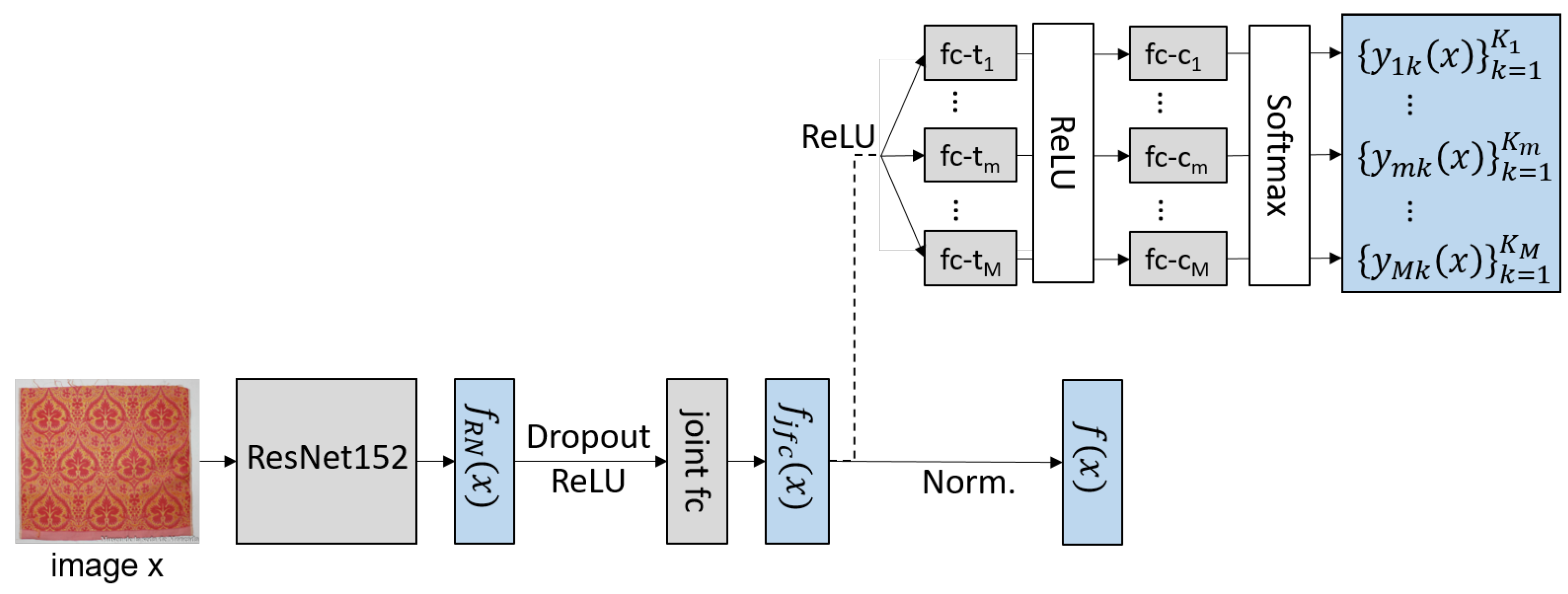
3.1. Network Architecture

The main objective of the CNN is to map an input image x to an image descriptor $f\left(x\right)$ to be used for image retrieval. For that purpose, the network architecture presented in Figure 1 is proposed. It consists of three main parts: a feature extraction part delivering features $f_{jfc}\left(x\right)$, an image retrieval head delivering the actual descriptor $f\left(x\right)$ and a classification head delivering normalized class scores $y_{mk}\left(x\right)$ that can be interpreted as posterior probabilities $P\left(C_{mk}\right|x)$ for the kth class of the mth semantic variable. The classification head exists only during training to allow for an auxiliary classification loss that is supposed to support descriptor learning.

The feature extraction part is a ResNet152 [56] backbone without the classification layer. It takes an RGB input image x of the size 224 by 224 pixels and calculates a 2048-dimensional feature vector $f_{RN}(x,{\mathbf{w}}_{RN})$, where ${\mathbf{w}}_{RN}$ denotes a vector containing all weights and biases of the ResNet152. The ResNet output $f_{RN}\left(x\right)$ is the argument of a ReLU (rectified linear unit [57]) nonlinearity and afterwards, a dropout [58] with a probability ${\rho }_d$ is applied. This is followed by $N{L}_{jfc}$ fully connected layers (joint fc in Figure 1) consisting of $N{N}_{jfc}$ nodes each. They are at the core of our method because the resulting feature vectors $f_{jfc}(x,{\mathbf{w}}_{RN},{\mathbf{w}}_{jfc})$ are the input to both the image retrieval and classification heads. Thus, the weights ${\mathbf{w}}_{jfc}$ of the joint fc layers are both influenced by the auxiliary multi-task classification loss as well as by the losses used for descriptor learning. Accordingly, it is assumed that the learned image representation $f_{jfc}(x,{\mathbf{w}}_{RN},{\mathbf{w}}_{jfc})$ is more meaningful with regard to the semantic annotations of the input image.

The image retrieval head consists of a simple normalization of the feature vector $f_{jfc}(x,{\mathbf{w}}_{RN},{\mathbf{w}}_{jfc})$ to unit length and does not require any further network weights. In the remainder of the paper, we use the shorthand ${\mathbf{w}}_{descr}:={[{\mathbf{w}}_{RN}^T,{\mathbf{w}}_{jfc}^T]}^T$ to denote the weights that have an influence on the descriptor. The result of normalization is the image descriptor $f(x,{\mathbf{w}}_{descr})$ to be used for image retrieval.

The image classification head takes the unnormalized vector $f_{jfc}(x,{\mathbf{w}}_{RN},{\mathbf{w}}_{jfc})=f_{jfc}(x,{\mathbf{w}}_{descr})$. After being processed by a ReLU activation, it is presented to M separate branches, each corresponding to one classification task to be learned; i.e., to the prediction of one of the M variables. Each branch is connected to the joint fc layer and consists of $N{L}_{f\mathit{c-}{t}_m}$ task-specific fully connected layers $fc$-$t_m$ of $N{N}_{f\mathit{c-}{t}_m}$ nodes, each with a ReLU. Finally, each branch has a classification layer $fc$-$c_m$ with $K_m$ nodes, where $K_m$ is the number of classes to be distinguished for the mth variable, delivering unnormalized class scores $a_{mk}\left(x,{\mathbf{w}}_{descr},{\mathbf{w}}_{class}\right)$. The weights ${\mathbf{w}}_{class}:={[{\mathbf{w}}_{f\mathit{c-}{t}_m}^T,{\mathbf{w}}_{f\mathit{c-}{c}_m}^T]}^T$ denote all weights in the classification head, where ${\mathbf{w}}_{f\mathit{c-}{t}_m}$ denotes the weights in the layers $fc$-$t_m$ and ${\mathbf{w}}_{f\mathit{c-}{c}_m}$ are the weights of the layers $fc$-$c_m$. All M classification layers have a softmax activation [59] delivering the normalized class scores $y_{mk}\left(x,{\mathbf{w}}_{descr},{\mathbf{w}}_{class}\right)$

$$y_{mk}\left(x,{\mathbf{w}}_{descr},{\mathbf{w}}_{class}\right)=\frac{exp\left(a_{mk}\left(x,{\mathbf{w}}_{descr},{\mathbf{w}}_{class}\right)\right)}{{\sum }_{j=1}^{K_m}exp\left(a_{mj}\left(x,{\mathbf{w}}_{descr},{\mathbf{w}}_{class}\right)\right)},$$

(1)

which can be interpreted as posterior probabilities $P\left(C_{mk}\right|x,{\mathbf{w}}_{descr},{\mathbf{w}}_{class})$; i.e., the network’s beliefs that the input image x belongs to class k for variable m.

3.2. Network Training

The training of the CNN depicted in Figure 1 is achieved by minimizing a loss function $\mathcal{L}\left(\mathbf{x},\mathbf{w}\right)$. The proposed CNN has two sets of parameters from the perspective of training: the weights ${\mathbf{w}}_{RN}$ of the ResNet152 and the remaining weights ${\mathbf{w}}_{head}:={[{\mathbf{w}}_{jfc}^T,{\mathbf{w}}_{class}^T]}^T$ of the additional layers. The weights ${\mathbf{w}}_{RN}$ are initialized by pre-trained weights obtained on the ILSVRC-2012-CLS dataset [60], whereas the weights ${\mathbf{w}}_{head}$ of the additional layers of the CNN are initialized randomly using variance scaling [61]. As it is expected that silk fabrics or other objects in the context of cultural heritage belong to another domain than objects depicted in the ImageNet dataset, the last residual blocks consisting of $N{L}_{RN}$ layers are potentially fine-tuned [62]. Denoting the parameters of the frozen ResNet layers by ${\mathbf{w}}_{R{N}_{fr}}$ and those of the fine-tuned ResNet layers by ${\mathbf{w}}_{R{N}_{ft}}$, the parameters to be determined in training are ${\mathbf{w}}_{tr}={[{\mathbf{w}}_{R{N}_{ft}}^T,{\mathbf{w}}_{head}^T]}^T$. Note that the entire parameter vector becomes $\mathbf{w}={[{\mathbf{w}}_{R{N}_{fr}}^T,{\mathbf{w}}_{tr}^T]}^T$.

Training is based on a set of training samples $\mathbf{x}$ that consist of images with semantic annotations for at least one of the M variables. In addition, the information that two or more images show the same object can be considered in training if available; for instance, the images can be exported from a database containing records about objects that are associated with multiple images [21]. Training is based on stochastic gradient descent mini-batch with adaptive moments [63]. In each training iteration, only a mini-batch ${\mathbf{x}}^{MB}$ consisting of $N^{MB}$ training samples is considered, and only the loss $\mathcal{L}\left({\mathbf{x}}^{MB},\mathbf{w}\right)$ achieved for the current mini-batch is used to update the parameters ${\mathbf{w}}_{tr}$. We use early stopping; i.e., the training procedure is terminated when the validation loss is saturated.

As the key idea of this paper is to support descriptor learning by simultaneously learning an auxiliary multi-task classifier in order to improve the clustering of the descriptors, the loss $\mathcal{L}\left({\mathbf{x}}^{MB},\mathbf{w}\right)$ consists of an image retrieval loss ${\mathcal{L}}_R\left({\mathbf{x}}^{MB},\mathbf{w}\right)$, a classification loss ${\mathcal{L}}_C\left({\mathbf{x}}^{MB},\mathbf{w}\right)$ and a regularization loss ${\mathcal{L}}_{wd}\left(\mathbf{w}\right)$:

$$\mathcal{L}\left({\mathbf{x}}^{MB},\mathbf{w}\right)={\lambda }_R·{\mathcal{L}}_R\left({\mathbf{x}}^{MB},\mathbf{w}\right)+{\lambda }_C·{\mathcal{L}}_C\left({\mathbf{x}}^{MB},\mathbf{w}\right)+{\mathcal{L}}_{wd}\left(\mathbf{w}\right).$$

(2)

The image retrieval loss ${\mathcal{L}}_R\left({\mathbf{x}}^{MB},\mathbf{w}\right)$ incorporates several similarity concepts to learn the trainable network weights ${\mathbf{w}}_{tr}$ based on a set of training samples ${\mathbf{x}}^{MB}$ such that the Euclidean distances of the descriptors $f\left(x_i\right),f\left(x_o\right)$ (cf. Figure 1) correspond to the degree of similarity of $x_i,x_o\in {\mathbf{x}}^{MB}$; this is described in detail in Section 3.2.1. The image classification loss ${\mathcal{L}}_C\left({\mathbf{x}}^{MB},\mathbf{w}\right)$ realizes a mathematical dependency of the weights $\mathbf{w}$ on the network’s ability to predict the correct class labels for all images $x_i\in {\mathbf{x}}^{MB}$. Thus, it can be seen as an auxiliary loss term for descriptor learning that supports the clustering of the descriptors with respect to the semantic properties of the depicted objects; details on that loss are presented in Section 3.2.2. The weights ${\lambda }_R$ and ${\lambda }_C$ in Equation (2) control the impact of the image retrieval and classification losses, respectively, on the total loss. Finally, ${\mathcal{L}}_{wd}\left(\mathbf{w}\right)$ denotes a weight decay term that is defined as [59]:

$${\mathcal{L}}_{wd}\left(\mathbf{w}\right)=\frac{\lambda }{2}·{\parallel {\mathbf{w}}_{tr}\parallel }^2=\frac{\lambda }{2}·\left({\mathbf{w}}_{tr}^T·{\mathbf{w}}_{tr}\right).$$

(3)

Adding weight decay to a loss function aims to avoid overfitting by penalizing large values of ${\mathbf{w}}_{tr}$. The parameter $\lambda$ controls the influence of the regularization term on the loss $\mathcal{L}\left({\mathbf{x}}^{MB},\mathbf{w}\right)$, as another hyperparameter to be tuned.

3.2.1. Image Retrieval Training Objective

The image retrieval loss should train the network by adapting the learnable parameters ${\mathbf{w}}_{tr}$ to produce descriptors such that for any pair of images $x_i,x_o$, the Euclidean distance ${\Delta }_{i,o,\mathbf{w}}^n$ of the corresponding descriptors $f(x_i,\mathbf{w})$ and $f(x_o,\mathbf{w})$ reflects the degree of similarity of the two images, where

$${\Delta }_{i,o,\mathbf{w}}^n=\left|\right|f(x_i,\mathbf{w})-f(x_o,\mathbf{w}){\left|\right|}_2,$$

(4)

where n is an index of a pair $x_i,x_o$ that will be defined differently for different loss functions. We propose a loss function that consists of three similarity loss terms:

$${\mathcal{L}}_R\left({\mathbf{x}}^{MB},\mathbf{w}\right)={\alpha }_{sem}·{\mathcal{L}}_{sem}\left({\mathbf{t}}^{MB},\mathbf{w}\right)+{\alpha }_{co}·{\mathcal{L}}_{co}\left({\mathbf{p}}_{co}^{MB},\mathbf{w}\right)+{\alpha }_{slf}·{\mathcal{L}}_{slf}\left({\mathbf{p}}_{slf}^{MB},\mathbf{w}\right).$$

(5)

Each of the three terms in Equation (5) corresponds to a specific concept of similarity and requires a specific type of training samples generated from the images of the mini-batch ${\mathbf{x}}^{MB}$. The loss term ${\mathcal{L}}_{sem}\left({\mathbf{t}}^{MB},\mathbf{w}\right)$, requiring a set ${\mathbf{t}}^{MB}$ of $N_t^{MB}$ triplets of training images from ${\mathbf{x}}^{MB}$, integrates semantic similarity into network training. The second term, ${\mathcal{L}}_{co}\left({\mathbf{p}}_{co}^{MB},\mathbf{w}\right)$, considers color similarity. It requires a set ${\mathbf{p}}_{co}^{MB}$ of $N_{co}^{MB}$ pairs of training images from ${\mathbf{x}}^{MB}$. Finally, ${\mathcal{L}}_{slf}\left({\mathbf{p}}_{slf}^{MB},\mathbf{w}\right)$ realizes the learning of self-similarity and requires a set ${\mathbf{p}}_{slf}^{MB}$ of $N_{slf}^{MB}$ pairs of images of the same object extracted from ${\mathbf{x}}^{MB}$. The impact of the individual loss terms on ${\mathcal{L}}_R\left({\mathbf{x}}^{MB},\mathbf{w}\right)$ is controlled by the weights ${\alpha }_{sem}$, ${\alpha }_{co}$, and ${\alpha }_{slf}$. The subsequent paragraphs contain a detailed description of all three similarity concepts as well as their integration into losses in the order in which they occur in Equation (5). The way in which the set ${\mathbf{t}}^{MB}$ of triplets and the sets ${\mathbf{p}}_{co}^{MB}$ and ${\mathbf{p}}_{slf}^{MB}$ of image pairs are determined given a mini-batch ${\mathbf{x}}^{MB}$ is described in detail in Section 3.3.

Semantic Similarity Loss

The goal of the semantic similarity loss is to learn the CNN parameters such that the resulting descriptors reflect the semantic similarity of the respective images. For that purpose, a concept of semantic similarity exploiting the class labels of M semantic variables is required. The degree of equivalence of the class labels of M variables assigned to an image pair $\left(x_i,x_o\right)$ can be measured by means of the semantic similarity defined in [21]:

$$Y_{sem}\left(x_i,x_o\right)=\frac{1}{M}·\sum _{m=1}^M{d}_m\left(x_i,x_o\right)·{\pi }_m^i·{\pi }_m^o.$$

(6)

In Equation (6), ${\pi }_m^q$ with $q\in \{i,o\}$ denotes whether the class label of the mth variable is known for the image with index q (${\pi }_m^q=1$) or not (${\pi }_m^q=0$). The actual comparison of the $K_m$ class labels of the mth variable in Equation (6) is realized by the function

$$d_m\left(x_i,x_o\right)=\sum _{k=1}^{K_m}\delta (l_{mk}\left(x_i\right)=l_{mk}\left(x_o\right)),$$

(7)

where ${\mathbf{l}}_m\left(x_q\right):={[l_{m1}\left(x_q\right),...,l_{mk}\left(x_q\right),...,l_{m{K}_m}\left(x_q\right)]}^T$ is a vector indicating the class label for the mth variable that is assigned to $x_q$, with $q\in \{i,o\}$. If the kth class of the mth variable is assigned to the image $x_q$, the indicator $l_{mk}\left(x_q\right)$ is 1; otherwise, $l_{mk}\left(x_q\right)=0$. Thus, the Kronecker delta function $\delta (·)$ returns 1 in case the kth class label is assigned to both $x_i$ and $x_o$, and it returns 0 in all other cases. This formalization of $d_m\left(x_i,x_o\right)$ implies that the label for the mth variable may be unknown either for $x_i$ or for $x_o$ or for both of them. If annotations for all variables are known, all values of ${\pi }_m^q$ will be 1, and $Y_{sem}\left(x_i,x_o\right)$ will correspond to the percentage of identical annotations for the two images. Consequently, the uncertainty about the equivalence of the class labels of the M variables depends on the percentage of variables for which either $x_i$ or $x_o$ has no annotation, which can be expressed as

$$u\left(x_i,x_o\right)=1-\frac{1}{M}·\sum _{m=1}^M{\pi }_m^i·{\pi }_m^o.$$

(8)

The goal of the semantic similarity loss is to learn the CNN parameters $\mathbf{w}$ such that the semantic similarity $Y_{sem}(x_i,x_o)$ of the image pair $(x_i,x_o)$ defined in Equation (6) corresponds to the descriptor similarity ${\Delta }_{i,o,\mathbf{w}}$ in Equation (4). For that purpose, the triplet loss [25] was adapted in [21], resulting in the semantic similarity loss

$${\mathcal{L}}_{sem}({\mathbf{t}}^{MB},\mathbf{w})=\frac{1}{N_t^{MB}}·\sum _{n_t=1}^{N_t^{MB}}max\left(M(x_i^{n_t},x_p^{n_t},x_n^{n_t})+{\Delta }_{i,p,\mathbf{w}}^{n_t}-{\Delta }_{i,n,\mathbf{w}}^{n_t},0\right).$$

(9)

The loss function in Equation (9) requires triplets $t^{n_t}:=(x_i^{n_t},x_p^{n_t},x_n^{n_t})$ with $t^{n_t}\in {\mathbf{t}}^{MB}$, each consisting of an anchor sample $x_i^{n_t}\in {\mathbf{x}}^{MB}$, a positive sample $x_p^{n_t}\in {\mathbf{x}}^{MB}$ and a negative sample $x_n^{n_t}\in {\mathbf{x}}^{MB}$, where $x_p^{n_t}$ is a sample that is more similar to the anchor sample than $x_n^{n_t}$. This loss forces $f\left(x_p^{n_t}\right)$ to have a Euclidean distance from $f\left(x_i^{n_t}\right)$ that is smaller than the distance of $f\left(x_n^{n_t}\right)$ from $f\left(x_i^{n_t}\right)$ by at least a margin of $M(x_i^{n_t},x_p^{n_t},x_n^{n_t})$:

$$M\left(x_i^{n_t},x_p^{n_t},x_n^{n_t}\right)=Y_{sem}(x_i^{n_t},x_p^{n_t})-\left(Y_{sem}(x_i^{n_t},x_n^{n_t})+u(x_i^{n_t},x_n^{n_t})\right)\stackrel{!}{>}0.$$

(10)

In Equation (10), $u(x_i^{n_t},x_n^{n_t})$ represents the uncertainty of the similarity status of the pair $(x_i^{n_t},x_n^{n_t})$ according to Equation (8). Thus, the term $Y_{sem}(x_i^{n_t},x_n^{n_t})+u(x_i^{n_t},x_n^{n_t})$ can be interpreted as the maximal positive semantic similarity of $x_i,x_n$ (i.e., assuming all missing annotations were identical), and the margin becomes the difference between the similarity $Y_{sem}(x_i^{n_t},x_p^{n_t})$ of the anchor and the positive sample and the maximum positive similarity of the anchor and the negative sample. Accordingly, $M\left(x_i^{n_t},x_p^{n_t},x_n^{n_t}\right)$ can be interpreted as the guaranteed difference in semantic similarity between the image pairs $(x_i^t,x_p^t)$ and $(x_i^t,x_n^t)$. The constraint $M\left(x_i^{n_t},x_p^{n_t},x_n^{n_t}\right)\stackrel{!}{>}0$ expressed in Equation (10) is considered in the definition of the set of triplets considered in this loss: only triplets of images fulfilling that constraint are eligible for contributing to this loss (cf. Section 3.3).

Color Similarity Loss

The goal of the color similarity loss is to learn the CNN parameters such that the resulting descriptors are similar for images with a similar color distribution and dissimilar for images with a different color distribution. The agreement between the color distributions of two images $x_i$ and $x_o$, denoted as color similarity, can be calculated by means of the normalized cross correlation coefficient $\rho (x_i,x_o)$ of color feature vectors $h\left(x_i\right)$ and $h\left(x_o\right)$ [21]:

$$\rho \left(x_i,x_o\right)=\frac{{\sum }_{j=1}^{l_h}(h_j\left(x_i\right)-\overline{h}\left(x_i\right))(h_j\left(x_o\right)-\overline{h}\left(x_o\right))}{\sqrt{{\sum }_{j=1}^{l_h}{(h_j\left(x_i\right)-\overline{h}\left(x_i\right))}^2·{\sum }_{j=1}^{l_h}{(h_j\left(x_o\right)-\overline{h}\left(x_o\right))}^2}},$$

(11)

where $h_j\left(x_q\right)$ is the $j^{th}$ element of $h\left(x_q\right)$ with $q\in \{i,o\}$, $l_h$ is the number of elements of a feature vector, and $\overline{h}\left(x_q\right)$ is the mean over all $h_j\left(x_q\right)$. The color feature vector $h\left(x_q\right)$ of an image $x_q$ describes the color distribution of that image in the HSV (H: hue, S: saturation, V: value) color space. To derive this feature vector, the hue H and saturation S values of every pixel of the image $x_q$ resized to 224 × 224 pixels are considered to be polar coordinates. They can be converted to Cartesian coordinates

$${\left[x^c(H,S),y^c(H,S)\right]}^T={\left[\frac{r}{2},\frac{r}{2}\right]}^T+\frac{r}{2}·S·{\left[cos(2\pi ·H),sin(2\pi ·H)\right]}^T,$$

(12)

so that all values of $x^c$ and $y^c$ are in the range $[0,r]$. We define a discrete grid consisting of $r\times r$ raster cells (we use r = 5) and count the number of points $(x^c(H,S),y^c(H,S))$ in each raster cell $(i^c,j^c)$. Finally, we concatenate the corresponding rows to form the vector $h\left(x_q\right)$. Thus, $h_j\left(x_q\right)$ is the number of points in the raster cell $(i^c,j^c)$, where $j=i^c+r·j^c$; this implies $l_h=r^2$ .

The correlation coefficient $\rho \left(x_i,x_o\right)\in [-1;1]$ expresses the linear dependency between the two color feature vectors $h\left(x_i\right)$ and $h\left(x_o\right)$. In case of identical color distributions of $x_i,x_o$ in HSV color space, the color descriptors $h\left(x_i\right),h\left(x_o\right)$ are identical and thus $\rho \left(x_i,x_o\right)$ becomes 1, indicating 100% color similarity. The lower the correlation coefficient, the lower the degree of similarity is supposed to be.

The color similarity loss aims to learn descriptors $f\left(x_i\right),f\left(x_o\right)$ whose Euclidean distance corresponds to the color similarity $\rho (x_i,x_o)$ of the image pair $(x_i,x_o)$ defined in Equation (11). This can be achieved by minimizing the following loss function [21]

$${\mathcal{L}}_{co}({\mathbf{p}}_{co}^{MB},\mathbf{w})=\frac{1}{N_{co}^{MB}}·\sum _{n_{co}=1}^{N_{co}^{MB}}max\left(0,|{\Delta }_{i,o,\mathbf{w}}^{n_{co}}-\left(1-\rho (x_i^{n_{co}},x_o^{n_{co}})\right)|\right).$$

(13)

This loss function requires pairs $p_{co}^{n_{co}}:=\left(x_i^{n_{co}},x_o^{n_{co}}\right)$ of images from the mini-batch, with $p_{co}^{n_{co}}\in {\mathbf{p}}_{co}^{MB}$; $N_{co}^{MB}$ is the number of pairs of images from ${\mathbf{x}}^{MB}$. Essentially, it forces the descriptor distance ${\Delta }_{i,o,\mathbf{w}}^{n_{co}}$ to be small for pairs of images with a large color similarity and to be large for image pairs of low similarity. If $\rho (x_i^{n_{co}},x_o^{n_{co}})=1$, indicating 100% color similarity of $x_i^{n_{co}}$ and $x_o^{n_{co}}$, the descriptor distance is forced to be zero; in the other extreme case of maximum dissimilarity—i.e., $\rho (x_i^{n_{co}},x_o^{n_{co}})=-1$—it should be ${\Delta }_{i,o,\mathbf{w}}^{n_{co}}=2$—i.e., the maximum possible descriptor distance given the fact that the descriptors are normalized to unit length (cf. Section 3.1).

Self-Similarity Loss

The goal of the self-similarity loss is to learn that the descriptors of images showing the same object are similar and thus to learn descriptors that are invariant to geometrical and radiometric transformations to some degree. Self-similarity means that an image $x_i$ is defined to be similar to an image $x_i^{\prime }$ that depicts the same object. This is the only similarity concept in our method that is not gradual. The corresponding loss requires the descriptor distances of all pairs $(x_i,x_i^{\prime })$ to be zero [21]:

$${\mathcal{L}}_{slf}({\mathbf{p}}_{slf}^{MB},\mathbf{w})=\frac{1}{N_{slf}^{MB}}·\sum _{n_{slf}=1}^{N_{slf}^{MB}}{\Delta }_{i,i^{\prime },\mathbf{w}}^{n_{slf}},$$

(14)

This loss function requires pairs $p_{slf}^{n_{slf}}:=(x_i^{n_{slf}},{x^{\prime }}_i^{n_{slf}})$ of images where $x_i^{n_{slf}}$ is an image of the mini-batch, with $p_{slf}^{n_{slf}}\in {\mathbf{p}}_{slf}^{MB}$. As there will be one such pair for every image $x_i^{n_{slf}}\in {\mathbf{x}}^{MB}$, we have $N_{slf}^{MB}=N^{MB}$. There are two options for the origin of ${x^{\prime }}_i^{n_{slf}}$ given an image $x_i^{n_{slf}}\in {\mathbf{x}}^{MB}$.

• If the dataset contains images showing the same object, ${x^{\prime }}_i^{n_{slf}}$ is selected to be one of these objects. This corresponds to rule 1 of the rule-based similarity proposed in [21]; note that the related rule-based loss of [21] is not considered in this paper.
• If the dataset contains no such images or if it is not known whether it contains such images, the image ${x^{\prime }}_i^{n_{slf}}$ is generated synthetically from $x_i^{n_{slf}}$, and in this case, the loss in Equation (14) could be seen as a variant of data augmentation; this is the only case considered in the self similarity loss of [21].

Compared to [21], the set of transformations potentially applied to $x_i^{n_{slf}}$ in the second case has been expanded. It includes the following geometrical transformations: a rotation of 90${}^{\circ }$, horizontal and vertical flips, cropping by a random percentage $b_{crop}\in [0.7;1]$ and small random rotations $\omega \in [-5^{\circ };+5^{\circ }]$. The set of potential radiometric transformations consists of a change of the hue $H\in [0;1]$ by adding a random value delta ${\Delta }_H\in [-0.05;+0.05]$ and an adaptation of the saturation S by multiplying it by a random factor ${\delta }_S\in [0.9;1.0]$. Finally, a random zero mean Gaussian noise with a standard deviation ${\sigma }_G=0.1$ can be added to generate the image ${x^{\prime }}_i^{n_{slf}}$.

As described above, we have expanded the concept of self-similarity in [21] by prioritizing images ${x^{\prime }}_i^{n_{slf}}$ extracted from the dataset over a synthetic generation of ${x^{\prime }}_i^{n_{slf}}$ for the definition of an image pair $(x_i^{n_{slf}},{x^{\prime }}_i^{n_{slf}})$.

3.2.2. Auxiliary Multi-Task Learning Training Objective

An auxiliary multi-task classification is supposed to support descriptor learning to generate clusters of image descriptors that better correspond to images of objects with similar semantic properties. As this loss affects the weights ${\mathbf{w}}_{descr}$ of the joint fc layers, it is expected to support the CNN in generating descriptors $f(x,{\mathbf{w}}_{descr})$ that represent variable-specific characteristics in the images $x\in {\mathbf{x}}^{MB}$ in a better way.

In [55], a multi-task classification loss for training a CNN to predict multiple variables related to images $x_i$ of silk fabrics was proposed:

$${\mathcal{L}}_{mtl}({\mathbf{x}}^{MB},\mathbf{w})=-\sum _{i=1}^N\sum _{m\in M_i}\sum _{k=1}^{K_m}{t}_{imk}·ln\left(y_{mk}\left(x_i,\mathbf{w}\right)\right).$$

(15)

It is an extension of the softmax-cross entropy for multi-task learning with missing annotations for M variables. In Equation (15), $y_{mk}\left(x_i,\mathbf{w}\right):=y_{mk}\left(x,{\mathbf{w}}_{descr},{\mathbf{w}}_{class}\right)$ denotes the softmax output for class k of variable m, $K_m$ is the corresponding number of classes and $t_{imk}$ is an indicator variable with $t_{imk}=1$ if k is the true class label of variable m for image $x_i$ and $t_{imk}=0$ otherwise. The second sum is only taken over variables $m\in M_i$, where $M_i$ is defined to be the subset of variables for which an annotation is available. In order to mitigate problems with underrepresented classes, we extend the loss in Equation (15) by a variant of the focal loss [64]. Whereas the variant presented [65] focuses on hard training examples in multi-class classification problems, we use a combination of the multi-class focal loss in [65] and the multi-task-loss in Equation (15), leading to the multi-task multi-class focal loss:

$${\mathcal{L}}_C({\mathbf{x}}^{MB},\mathbf{w})=-\frac{1}{N_M^{MB}}\sum _{i=1}^N\sum _{m\in M_i}\sum _{k=1}^{K_m}{\left(1-y_{mk}\left(x_i,\mathbf{w}\right)\right)}^{\gamma }·t_{imk}·ln\left(y_{mk}\left(x_i,\mathbf{w}\right)\right).$$

(16)

In Equation (16), $N_M^{MB}$ is the number of available annotations for all M variables; i.e., $N_M^{MB}:={\sum }_{i=1}^N{\sum }_{m\in M_i}{\sum }_{k=1}^{K_m}{t}_{imk}$. The focusing parameter $\gamma$ controls the influence of the focal weight $(1-y_{mk}\left(x_i,\mathbf{w}\right))\in [0,1]$ on the loss ${\mathcal{L}}_C({\mathbf{x}}^{MB},\mathbf{w})$. As the focal weight becomes 1 for $y_{mk}\left(x_i,\mathbf{w}\right)\to 0$ and the focal weight becomes 0 for $y_{mk}\left(x_i,\mathbf{w}\right)\to 1$, the loss ${\mathcal{L}}_C({\mathbf{x}}^{MB},\mathbf{w})$ depends more strongly on $x_i\in {\mathbf{x}}^{MB}$ with small softmax scores $y_{mk}\left(x_i,\mathbf{w}\right)$. Thus, the network weights ${\mathbf{w}}_{tr}$ are influenced more strongly by hard training examples indicated by small $y_{mk}\left(x_i,\mathbf{w}\right)$ for $t_{nmk}=1$ when minimizing ${\mathcal{L}}_C({\mathbf{x}}^{MB},\mathbf{w})$. Assuming class imbalances for the class distributions of at least one of the M variables, the focal loss in Equation (16) is supposed to improve the classification performance of underrepresented classes as the class scores of such classes are generally low, thus also supporting the CNN to produce descriptors which are more likely to help in retrieving images with similar semantic properties for query images corresponding to underrepresented classes for some variables.

3.3. Batch Generation

This section gives an overview of how a mini-batch of images ${\mathbf{x}}^{MB}$ with related class labels as well as potential information indicating images that depict the same object is processed in order to generate the datasets required by the individual loss terms. In general, the auxiliary classification loss requires a set of independent images, whereas the loss terms in the image retrieval loss need sets of pairs or triplets of images in order to learn similarity; i.e., to produce descriptors whose pairwise Euclidean distance reflect similarity. These sets are generated as follows:

• The semantic similarity loss ${\mathcal{L}}_{sem}({\mathbf{t}}^{MB},\mathbf{w})$ in Equation (9) requires triplets $t=(x_i,x_p,x_n)$∈${\mathbf{t}}^{MB}$. In a first step, all possible triplets with $x_i\ne x_p\ne x_n$ are generated for every image $x_i\in {\mathbf{x}}^{MB}$. As for a triplet to be valid, the positive sample $x_p$ has to be more similar to $x_i$ than the negative sample $x_n$, only those $N_t^{MB}$ triplets fulfilling the constraint related to the margin formulated in Equation (10) are presented to the network. As the number of $N_t^{MB}$ is dependent on the margin $M\left(x_i^{n_t},x_p^{n_t},x_n^{n_t}\right)$ calculated from the available class labels in a mini-batch, the loss is normalized by the number of triplets.
• The color similarity loss ${\mathcal{L}}_{co}\left({\mathbf{p}}_{\mathbf{c}}^{\mathbf{MB}},\mathbf{w}\right)$ in Equation (13) requires pairs of images $p_{co}=(x_i,x_j)\in {\mathbf{p}}_{co}^{MB}$. For that purpose, all possible pairs $p_{co}$ in the mini-batch ${\mathbf{x}}^{MB}$ are generated, excluding all pairs $p_{co}=(x_i,x_j)$ with $i=j$. Thus, the color similarity loss is calculated for $N_{co}^{MB}=N_{MB}!/\left(2!·(N_{MB}-2)!\right)$ pairs of training samples, where ! denotes the factorial of a number.
• The self similarity loss ${\mathcal{L}}_{slf}({\mathbf{p}}_{slf}^{MB},\mathbf{w})$ requires pairs of images $p_{slf}=(x_i,x_i^{\prime })\in {\mathbf{p}}_{slf}^{MB}$. There is one such pair per image in the mini-batch; as described in Section 3.2.1, if there exist other images in the dataset that show the same object as $x_i$, one of these images is randomly chosen to serve as the partner $x_i^{\prime }$. Otherwise, $x_i^{\prime }$ is generated synthetically using a randomly drawn transformation as defined in Section 3.2.1.
  This results in $N_{slf}^{MB}=N_{MB}$ pairs of images $p_{slf}$.
• The classification loss ${\mathcal{L}}_C\left({\mathbf{x}}^{MB},\mathbf{w}\right)$ in Equation (16) requires a set of independent images $x\in {\mathbf{x}}^{MB}$ with known classes for ideally all of the M variables in order to learn $\mathbf{w}$ such that the predictions $y_k$ become optimal. Accordingly, all $N_{MB}$ images in the mini-batch can be presented to the classification loss. As class labels are potentially not available for all M variables, there are potentially less than $N_{MB}·M$ cross-entropy terms constituting the classification loss in case of mutually exclusive class labels per variable. Thus, the loss is normalized by the number of known class labels $N_M^{MB}$ for the M variables; i.e., the number of terms constituting the loss.

Due the normalization of all loss terms by the number of terms of the sum in the individual loss functions, the total loss is not biased towards loss terms with a larger number of summands.

4. Dataset

This section describes the datasets that are used to evaluate the methodology described in Section 3. The first dataset, referred to as the SILKNOW dataset, is introduced in Section 4.1. It contains images of silk fabrics and is used for a thorough evaluation of the proposed image retrieval approach. The second dataset, described in Section 4.2, is a variant of the WikiArt dataset and contains images of paintings from the last few centuries. This dataset is used to analyze the transferability of the proposed methodology to other cultural heritage datasets.

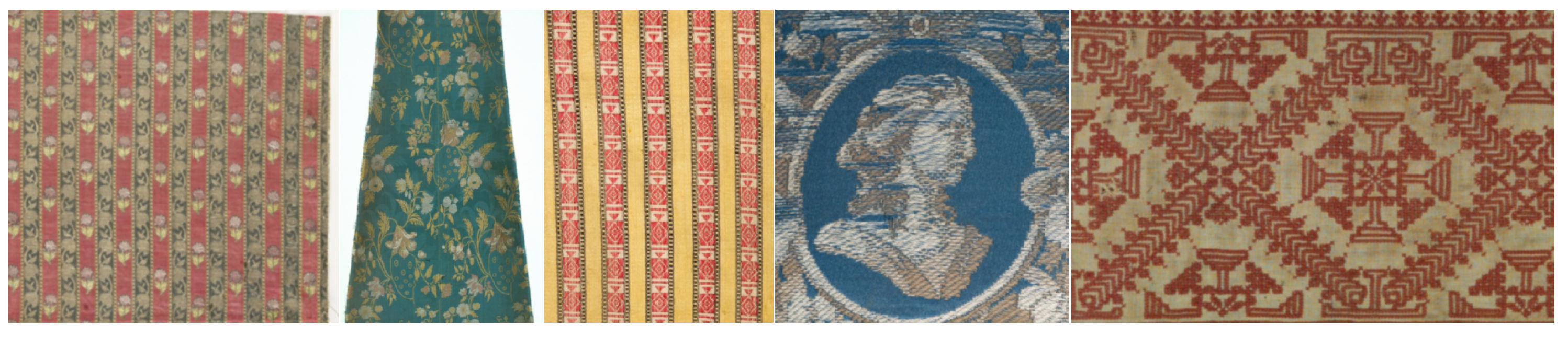
4.1. SILKNOW Dataset

The SILKNOW dataset is based on the SILKNOW knowledge graph [1,21] that was generated in the frame of the EU-H2020 project SILKNOW with the goal of building and providing a platform (https://ada.silknow.org/, visited on 30 November 2021) containing information about European silk cultural heritage. The graph contains records of plain silk fabrics as well as processed textiles, harvested from online collections of a variety of museums; e.g., the Museu Tèxtil de Terrassa (IMATEX dataset) [66] or the Boston Museum of Fine Arts. Each record corresponds to one artifact, and many of the records contain at least one image. The semantic information available at the harvested websites was mapped to a standardized format in the context of the SILKNOW project on the basis of a thesaurus, which is another outcome of the project. In addition, there is a mapping of the available information to a simplified class structure for the variables material, place, timespan and technique that forms the basis for the dataset used in this paper.

The SILKNOW dataset used in this paper was exported from the SILKNOW knowledge graph. It consists of 48,830 images of plain fabrics, with each image being associated with a valid annotation in at least one of the four variables mentioned above. To avoid strongly underrepresented classes, only labels occurring at least 150 times are considered valid. In addition, a unique object identifier is associated with every image, so that the information required to identify images showing the same object,used in the definition of image pairs for the self-similarity loss (cf. Section 3.2.1) is available. For the purpose of evaluating the methodology presented in Section 3, the dataset was randomly split into a training set (60%), a validation set (20%) and a test set (20%). The training set was further split into a subset of images used for updating the trainable weights and another subset used for early stopping. The statistics of the class distributions in all variables and all subsets are listed in

Table 1. Statistics of the distribution of samples for the SILKNOW dataset. Variable: name of the variable considered; the number beneath the class names are percentages of samples with annotation for that variable. Class name: classes differentiated for each variable; total: number of samples for a class; train: number of samples used for training; update: number of training samples used for weight updates; stop: number of training samples used for early stopping; val: number of samples in the validation set; test: number of samples in the test set.

Variable	Class Name	Total	Train	Update	Stop	Val	Test
material	animal fibre	27,252	16,700	12,546	4154	5330	5222
(72.4%)	metal thread	4208	2574	1943	631	684	950
	vegetal fibre	3891	2407	1763	644	707	777
place	GB	7998	5154	3908	1246	1282	1562
(71.3%)	FR	7379	4452	3346	1106	1527	1400
	ES	4708	2847	2127	720	921	940
	IT	4700	2781	2131	650	995	924
	IN	2353	1441	1069	372	420	492
	CN	1399	866	636	230	276	257
	IR	1294	802	608	194	248	244
	JP	1097	794	588	206	163	140
	BE	648	405	305	100	71	172
	TR	593	342	240	102	94	157
	DE	592	388	291	97	96	131
	GR	479	281	206	75	69	129
	NL	455	310	226	84	85	60
	US	357	238	190	48	54	65
	PK	352	225	165	60	67	60
	RU	228	137	99	38	46	45
	JM	191	105	77	28	49	37
timespan	19th century	9975	6041	4569	1472	1938	1996
(57.9%)	18th century	8423	5155	3819	1336	1539	1729
	20th century	4012	2447	1821	626	778	787
	17th century	3378	2170	1649	521	482	726
	16th century	1829	1154	873	281	332	343
	15th century	685	433	338	95	100	152
technique	embroidery	6861	4333	3237	1096	1217	1310
(32.2%)	velvet	3051	1854	1422	432	671	526
	damask	2768	1615	1218	397	582	571
	other technique	2526	1585	1203	382	463	478
	resist dyeing	355	289	213	76	15	51
	tabby	185	98	70	28	37	50

.

As the statistics in Table 1 indicate, the dataset is unbalanced, which makes it challenging. Depending on the variable, the amount of available class labels varies between 32.2% for technique and 72.4% for material. Of the images in the dataset, 6143 have annotations for all of the four variables. For 13,771 of the images, class labels are known for three of the four variables, and there are 19,421 images with annotations for two variables. Furthermore, the number of classes to be differentiated varies between 3 classes for material and 17 classes for the variable place. Examples of images of plain silk fabrics can be seen in Figure 2.

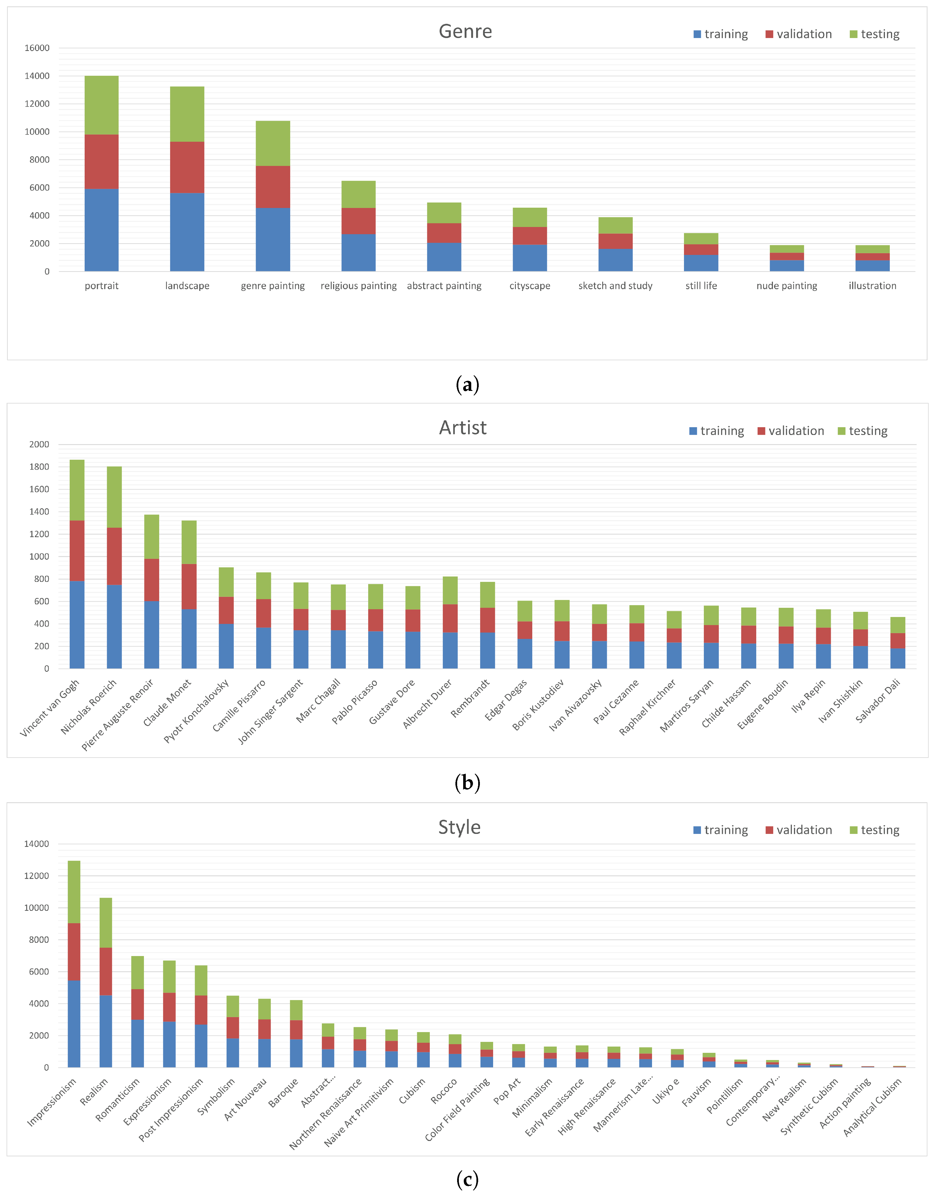
4.2. WikiArt Dataset

In recent years, many works have investigated the image classification of cultural heritage collections, most of which have dealt with the classification of images of paintings, such as those in the WikiArt dataset. As the WikiArt dataset consists of images as well as annotations for several semantic variables, it is not only suitable for evaluating classification tasks but also fulfills the requirements of our image retrieval method. Thus, we chose the WikiArt dataset to demonstrate the transferability of our approach to other non-silk digital collections in the context of cultural heritage. As the WikiArt dataset is continuously growing over time, we decided to use the version of WikiArt (https://github.com/cs-chan/ArtGAN/tree/master/WikiArt%20Dataset, visited on 30 November 2021) provided by the authors of [40]. They not only published the image data (81,444 images in total) and related class labels for the three variables genre, style and artist, but also their data were split for training and validation for each variable. We use the same split and perform the network training as well as the hyperparameter tuning on their training set, whereas their validation set was used exclusively for testing the trained and tuned model.

In contrast to the single-task learning experiments in [40], we consider a multi-task learning objective in the context of image retrieval, and we also define similarity based on multiple variables. Consequently, we refine the provided data splits by eliminating images that occur both in the training and in the validation sets for any variable. Thus, we obtain a data set of 80,880 images with up to three class labels per image (one per variable) with disjoint training and validation sets. Furthermore, we split the training set into two disjoint subsets; one for network training and one for hyperparameter tuning. In the remainder of this paper, we denote the subset for network training as the training set and the subset for hyperparameter tuning as the validation set. The set referred to as the validation set in [40] is called our test set. Analogous to the SILKNOW dataset, the training dataset is also divided into two independent subsets: update, consisting of 75% of the training samples for the weight updates, and stop, consisting of the remaining 25% of samples for early stopping.

The resulting class structures as well as the class distributions of the three semantic variables genre, artist and style in our multi-task WikiArt dataset can be found in Figure 3. For the variable genre, 10 classes are differentiated, with the number of samples per class varying between 1879 for the class illustration and 14,010 for the class portrait. For the variable artist, there are 23 classes, where the minimum and maximum number of samples are 461 (Salvador Dali) and 1864 (Vincent van Gogh), respectively. Finally, there are 27 different style classes with a minimum of 106 (Analytical Cubism) and a maximum of 12,941 images per class (Impressionism). It is worth mentioning that a class label for the variable artist is available for 23.2% of the 80,880 images in the multi-task dataset, the information about the genre of the depicted painting is available for 79.7% of the images, and only the style information is known for all of the images. Examples for images in the WikiArt dataset are shown in Figure 4.

5. Experiments and Results

In this section, the methodology for learning descriptors for image retrieval described in Section 3 is evaluated. We start with an overview of the conducted experiments and a description of the evaluation strategy for comparing the results of different experiments (Section 5.1). An ablation study investigating the impact of the different components of the proposed approach can be found in Section 5.2. All of these experiments are based on the SILKNOW dataset (cf. Section 4.1), which corresponds to the use case for which the methodology was mainly developed. To show the transferability of the method to other labeled datasets, an evaluation on the version of the WikiArt dataset described in Section 4.2 was also performed. The results are reported in Section 5.3.

5.1. Test Setup and Evaluation Strategy

In order to train the CNN presented in Section 3.1, the training sets of the datasets as defined in Section 4 are used to determine the network weights ${\mathbf{w}}_{tr}$, whereas the validation set was used to find optimal hyperparameters. The test sets are used for an independent evaluation, the results of which are reported in the subsequent sections.

5.1.1. General Test Setup

In the training process, the loss presented in Equation (2) is minimized by means of stochastic mini-batch gradient descent [59] with a batch size of $N_{MB}=300$ utilizing the Adam optimizer [63] using the standard parameters ($\alpha =1\times {10}^{-3}$, ${\beta }_1=0.9$, ${\beta }_2=0.999$ and $\widehat{ϵ}=1\times {10}^{-8}$) until the loss on an independent subset of the training data denoted as stop in Section 4 is saturated.

A series of preliminary experiments—not reported here for lack of space—was used to tune the hyperparameters of our method by assessing the results on the validation set. All of these were conducted on the SILKNOW dataset; in the experiments based on the WikiArt dataset, the same parameters were used. As far as the CNN structure was concerned, it was found that using one fully connected layer with 256 nodes for joint fc—i.e., using $N{L}_{jfc}=1$ and $N{N}_{jfc}=256$—is to be preferred over variants with more layers or more nodes per layer. The optimal architecture for the $M=$ classification branches was found to consist of $N{L}_{f\mathit{c-}{t}_m}=1$ layer with $N{N}_{f\mathit{c-}{t}_m}=128$ nodes. The hyperparameter tuning confirmed that using a learning rate $\alpha$ of $1\times {10}^{-3}$ is also a good choice for our application; the optimal values for the dropout rate was ${\rho }_d=0.3$, for weight decay, it was $\lambda =1\times {10}^{-3}$, and _for the parameter in the focal loss (Equation (16)), it was $\gamma =1$. Somewhat surprisingly, the fine-tuning of the last residual blocks of the ResNet152 backbone did not improve the performance; consequently, the number of layers to be fine-tuned was set to $N{L}_{RN}=0$, which implies that the weights ${\mathbf{w}}_{RN}$ determined in pre-training remain unchanged. As a result, the vector ${\mathbf{w}}_{R{N}_{ft}}$ of fine-tuned ResNet parameters is a zero vector, and the vector of trainable parameters is ${\mathbf{w}}_{tr}={\mathbf{w}}_{head}$ (cf. Section 3.2).

5.1.2. Test Series

Section 5.2 and Section 5.3 show the experimental results of two series of experiments. In a first series performed on the SILKNOW dataset (cf. Section 4.1), the impact of the individual loss terms constituting $\mathcal{L}\left(\mathbf{x},\mathbf{w}\right)$ (Equation (2)) on the image retrieval results is evaluated. This test series also indicates our method’s potential to produce descriptors for image retrieval in the use-case for which it was originally designed. For that purpose, different values for ${\lambda }_C,{\lambda }_R$ as well as different values for ${\alpha }_{sem},{\alpha }_{co} \mathrm{and} {\alpha }_{slf}$ are investigated.

Table 2. Overview of the experiments conducted in the ablation study on the SILKNOW dataset. First column: name by which the experiment is identified (Experiment). The other columns give the weights of the loss function terms for each experiment. The weights ${\lambda }_C$ and ${\lambda }_R$ control the impact of the retrieval loss and the auxiliary classification loss, respectively, on the total loss in Equation (2); ${\alpha }_{sem},{\alpha }_{co}$ and ${\alpha }_{slf}$ control the impact of the individual similarity loss terms on the retrieval loss in Equation (5). The names of the experiments refer to the loss terms that were considered (sem: semantic similarity loss ${\mathcal{L}}_{sem}$, co: color similarity loss ${\mathcal{L}}_{co}$, slf: self-similarity loss ${\mathcal{L}}_{slf}$), C: classification loss ${\mathcal{L}}_C$). Comparing the results with and without the classification loss shows its impact on the results.

Experiment	${\mathit{\lambda }}_{\mathit{R}}$	${\mathit{\lambda }}_{\mathit{C}}$	${\mathit{\alpha }}_{\mathit{sem}}$	${\mathit{\alpha }}_{\mathit{co}}$	${\mathit{\alpha }}_{\mathit{slf}}$
sem	1	0	1.0	0.0	0.0
co	1	0	0.0	1.0	0.0
sem + co	1	0	0.5	0.5	0.0
sem + slf	1	0	1.0	0.0	0.5
sem + co + slf	1	0	0.5	0.5	0.5
sem + C	1	1	1.0	0.0	0.0
sem + co + C	1	1	0.5	0.5	0.0
sem + slf + C	1	1	1.0	0.0	0.5
sem + co + slf + C	1	1	0.5	0.5	0.5

gives an overview over the conducted experiments, identifying each of them by a name and giving the corresponding parameter settings. In order to allow for a better interpretation of the differences in performance given the random components of the training procedure, each experiment is executed five times, resulting in average evaluation metrics and a corresponding standard deviation.

The parametrization of the loss function of the variant identified to be the best one in the first series of experiments is chosen for the experiments in the second test series, in addition to a variant in which all loss terms contribute to the total loss. The second series should show the transferability of the results to other applications than the one it was originally designed for. Unfortunately, we could not find any studies to which a fair comparison of our method is possible, because in the context of uni-modal image retrieval for cultural heritage applications, we are unaware of any paper for which both the results and the datasets used to achieve them are available.

Evaluation Strategy

It is not straightforward to evaluate an image retrieval method if no samples of pairs of images with a known similarity status is known. However, the main goal of the method presented in this paper is to retrieve images with similar semantic properties to those of the query image. Consequently, the available semantic annotations of a set of reference samples (the test set of the corresponding dataset used for evaluation) can be used for a quantitative evaluation. Thus, the image retrieval results are used for a k nearest neighbor (kNN) classification with $k=10$, and the evaluation is based on the corresponding classification results. After training the network, the descriptors of the images in the training set are computed. These descriptors are considered to represent the set of images in which a user wants to search for semantically similar images; they are organized in a kd-tree [2] for a fast kNN search. The images of the test set are considered to be the query images. For each of them, a descriptor is computed, and the $k=10$ nearest neighbors are retrieved from the kd-tree, with the results giving access to the k most similar images in the training set. A majority vote among the class labels of the retrieved images gives the class label of a query image for all variables, and these labels can be compared to the reference labels for a quantitative evaluation.

For all experiments, we report the overall accuracy (OA) describing the percentage of correctly classified images among all evaluated images. In this context, the OA of the mth variable is computed exclusively based on images with a known class label for variable m, taking into account the fact that some annotations may be missing for a query image. As the class distributions of all M variables of the two datasets are very imbalanced, we further report the mean F1 score per variable; i.e., the arithmetic mean of all class-specific F1 scores. The class-specific F1 score is the harmonic mean of precision (indicating the percentage of predictions of a class that actually belong to that class) and recall (indicating the percentage of samples per class in the reference that were predicted by the CNN). Thus, in contrast to the OA, the mean F1 scores are not biased by dominant classes in the dataset. All of these evaluation metrics are presented separately for the validation and the test sets.

5.2. Results of the Experiments Using the SILKNOW Dataset

The results of the first series of experiments, conducted on the SILKNOW dataset, can be found in

Table 3. Results of the experiments conducted on the SILKNOW dataset. The quality metrics are averaged over all four variables. Each experiment was executed five times, leading to the presented means mean and standard deviations std on the test set. The names of the experiments are those presented in Table 2.

Quality Metric	Experiment	Mean	Std
OA [%]	sem	61.2	0.18
	co	54.7	0.20
	sem + co	60.9	0.17
	sem + slf	53.5	0.34
	sem + co + slf	56.5	0.21
	sem + C	63.9	0.11
	sem + co + C	63.7	0.11
	sem + slf + C	62.2	0.16
	sem + co + slf + C	62.2	0.15
F1 score [%]	sem	37.3	0.34
	co	32.1	0.39
	sem + co	38.0	0.48
	sem + slf	29.2	0.30
	sem + co + slf	32.4	0.51
	sem + C	42.9	0.31
	sem + co + C	42.7	0.30
	sem + slf + C	40.2	0.36
	sem + co + slf + C	40.0	0.40

,

Table 4. Overall accuracies [%] of the experiments conducted on the SILKNOW dataset. The average performance on the test dataset over five executions per experiment is presented per variable. See Table 2 for the names of the experiments.

Experiment	Material		Place		Timespan		Technique
	mean	std	mean	std	mean	std	mean	std
sem	75.0	0.16	46.0	0.23	54.9	0.58	68.9	0.60
co	74.3	0.10	37.8	0.54	47.9	0.77	58.9	0.63
sem + co	74.9	0.25	46.1	0.41	54.3	0.36	68.4	0.50
sem + slf	74.2	0.29	35.4	0.22	46.0	1.14	58.4	0.36
sem + co + slf	74.3	0.31	39.5	0.80	49.8	0.58	62.3	0.62
sem + C	75.0	0.23	49.2	0.34	58.7	0.31	72.6	0.24
sem + co + C	75.1	0.16	49.3	0.11	58.6	0.44	71.7	0.26
sem + slf + C	74.8	0.27	47.5	0.44	56.5	0.81	69.9	0.61
sem + co + slf + C	74.7	0.09	47.5	0.31	56.9	0.39	69.7	0.38

and

Table 5. Mean F1 scores per variable [%] of the experiments conducted on the SILKNOW dataset. The average performance on the test dataset over five executions per experiment is presented per variable. See Table 2 for the names of the experiments.

Experiment	Material		Place		Timespan		Technique
	mean	std	mean	std	mean	std	mean	std
sem	36.4	0.50	22.9	0.24	43.2	0.52	46.6	1.66
co	34.1	0.23	18.4	0.33	35.8	0.90	39.9	0.78
sem + co	37.3	0.67	23.7	0.75	42.4	0.42	48.5	1.51
sem + slf	33.7	1.20	14.8	0.62	31.6	0.74	36.7	0.50
sem + co + slf	34.9	0.77	17.4	0.51	36.5	0.52	40.9	1.58
sem + C	40.2	0.48	29.1	0.62	47.4	0.60	55.0	1.36
sem + co + C	40.3	0.51	28.9	0.53	47.4	0.76	54.3	0.77
sem + slf + C	39.5	0.59	27.3	0.48	44.7	1.23	49.2	1.10
sem + co + slf + C	38.8	0.20	26.2	0.60	44.7	0.39	50.3	1.21

. Whereas Table 3 focuses on the average OAs and the average F1 scores per experiment, Table 4 gives insights into the OAs per variable, and Table 5 presents the mean F1 scores per variable.

5.2.1. General Observations

The results in Table 3 give a first impression of how the individual loss terms affect the performance of the presented approach to retrieve images that are semantically similar to the query image. The experiments and the corresponding evaluation metrics consist of three groups; the first group consists of experiments exclusively training the CNN by optimizing one of the two main loss terms ${\mathcal{L}}_{sem},{\mathcal{L}}_{co}$ of the image retrieval loss ${\mathcal{L}}_R$, the second group contains experiments based on different combinations of the loss terms constituting the image retrieval loss ${\mathcal{L}}_R$, and the third group combines all variants of the second group with the classification loss ${\mathcal{L}}_C$. Unsurprisingly, the metrics obtained in the first group of experiments show that training based on semantic similarity yields better results in an evaluation focusing on semantic aspects. On average, in 61.2% of the cases, a majority vote among the k retrieved images delivers the correct class label if ${\mathcal{L}}_{sem}$ is used for training, which is 6.2% more than can be achieved when only using color similarity (sem vs. co). There is also a relatively large difference in mean F1 scores (5.2%). The results of the second group of experiments show that the combination of semantic and color similarity (sem + co) is on par with the variant based on semantic similarity only (sem) in terms of OA; the difference of 0.3% is not significant considering that the standard deviation of OA is in the order of 0.2%. The difference in mean F1 scores is slightly larger, but again it is statistically not significant. Interestingly, and somewhat surprisingly, the inclusion of the self similarity loss seems to have a considerable negative impact on the results in this group of experiments. Finally, the third group of experiments shows that, on average, the combination of the image retrieval loss ${\mathcal{L}}_R$ with the image classification loss ${\mathcal{L}}_C$ outperforms all variants of the first and second groups.

The two best loss variants are identified to be sem + C, combining the semantic image retrieval loss with the image classification loss, and sem + co + C combining the semantic and color image retrieval losses with the image classification loss. The difference between these two variants (0.2% in both OA and mean F1 score) are insignificant. Correctly predicting the class labels of test images in 63.9% of the cases, variant sem + C outperforms its corresponding variant without classification loss (sem) by 2.7% in OA. As the standard deviations of the OAs are in the range of up to 0.2%, this improvement is considered to be significant. The mean F1 score was improved by about 5.6%, which is also a significant improvement considering the standard deviations of around 0.3% for the mean F1 scores in these experiments. The trend for the variant also considering the color loss (sem + co + C) is similar when compared to variant sem; the improvement compared to variant sem + co in OA is slightly larger because that variant had a slightly worse OA than variant sem, and it is slightly smaller in terms of the mean F1 score (4.7%) because sem + co performed better than sem in that metric. Interestingly, the inclusion of the classification loss mitigates the negative influence of the self similarity loss, though it cannot completely compensate it. From this analysis, we can conclude that the inclusion of the classification loss leads to a significant improvement of the average performance of our method to retrieve images that are semantically similar to the query image. In OA, the improvement is 2.7% in the best scenario. The improvement in the mean F1 score is larger (5.6%), which we take as a first indication that the classification loss particularly mitigates problems with underrepresented classes.

5.2.2. Variable-Specific Analysis

A more detailed analysis of the OAs can be made based on Table 4, showing the OA achieved on the SILKNOW test set per semantic variable. Comparing the obtained OAs of the individual variables, it is obvious that the classes of some variables can be predicted much better than those of other variables. Considering the class structures of the four variables, one can infer that higher OAs can be obtained for variables with fewer classes to be distinguished; the variable place, with 17 classes, obtains the lowest accuracies, whereas the variable material with only three classes obtains the highest accuracies (about 75%), which is about 30% higher than the values achieved for place. The two variants sem + C and sem + co + C result in the highest OAs for all of the four variables, which is consistent with the average values in Table 3. Table 4 shows that the variable material—i.e., the one for which the best results are achieved—is hardly affected by the methodological changes between the experiments. In particular, there is no difference in performance between the experiments sem, sem + C and sem + co + C; all of them result in an OA of 75%. For the other two variables, there is a larger improvement due to the inclusion of the classification loss. In all of the cases, the variants sem and sem + C achieve similar OA values; including the classification loss leads to an improvement of the OA by 3.2%–3.8%.

Analyzing the mean F1 scores per variable in Table 5 confirms that the two experiments sem + C and sem + co + C result in the highest quality metrics for all four variables. Comparing the mean F1 scores obtained in the two best experiments in Table 5 with the corresponding OAs in Table 4, large differences of about 10% (timespan) to 35% (material) can be observed. This indicates remaining problems with underrepresented classes. Comparing the mean F1 scores of the individual classes in the best experiments, there is not such an obvious dependency of the performance on the number of classes to be distinguished for a variable as can be observed for the overall accuracy. Even though the lowest F1 scores of up to 29.1% are still obtained for place, with the largest number classes, the highest scores of up to 55.0% are obtained for the variable technique, followed by timespan, both having six classes. A possible reason could be that different manufacturing techniques of silk fabrics may lead to the largest visual variations in the images, and thus it might be easier to distinguish the individual classes of technique by means of learned image representations produced by the trained CNN. Comparing the best performing variants (sem + C and sem + co + C) with their corresponding counterparts, not considering the classification loss (sem and sem + co), the largest difference in mean F1 score amounts to 8.4% (technique). For the other variables, the improvement varies between 3.9% (material) and 6.3% place, in all cases being significant given the standard deviation of the mean F1 score in the order of 0.5%. Thus, the analysis confirms the significant positive impact of the auxiliary classification loss on the ability of our method to retrieve images with semantic properties similar to those of the query image. As the improvement in the mean F1 scores is larger than that in the OAs, we believe that this is mainly due to a positive contribution to the differentiation of underrepresented classes, although some problems still remain, as indicated by the gap between OA and mean F1 scores.

In summary, the experiments in the first test series show that the combination of the semantic similarity loss with losses related to other similarity concepts—i.e., color similarity and self-similarity—does not improve the network’s ability to produce descriptors that can be used to retrieve images having semantic properties similar to those of the query image. In contrast, adding an additional classification loss significantly improves both the mean F1 scores and the OAs.

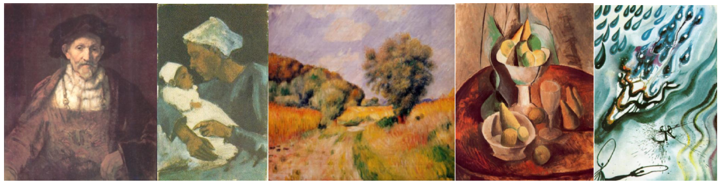
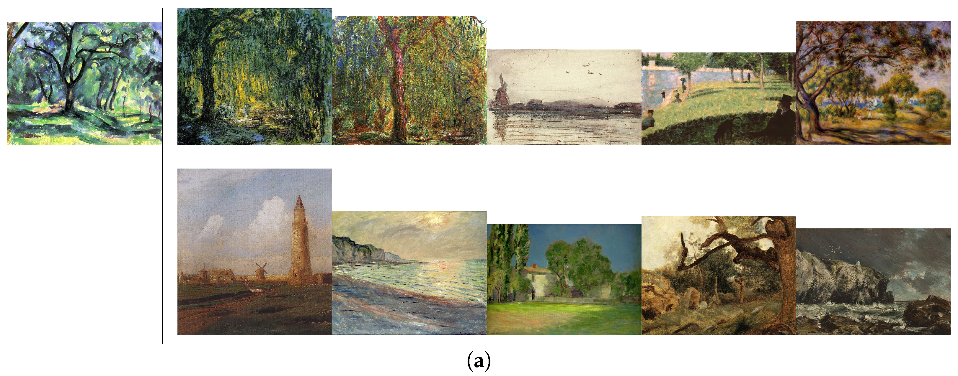
5.3. Transferability of the Approach: Evaluation on the WikiArt Dataset

The results of the second series of experiments, based on the WikiArt dataset utilizing the best model variant in terms of the F1 score identified in the preceding section as well as the variant using all loss terms sem + co + slf + C, can be found in

Table 6. Quality metrics of two model variants on the WikiArt test dataset.

Quality Metric	Model	Style	Genre	Artist	Average
OA [%]	sem + C	43.0	69.9	54.5	55.8
	sem + co + slf + C	40.6	67.6	50.7	53.0
F1 score [%]	sem + C	37.3	64.7	51.2	51.1
	sem + co + slf + C	33.1	62.1	47.1	47.4

. The table provides both information about the percentage of correctly classified images per variable (overall accuracy) as well as the variable-specific mean F1 scores. Comparing the two investigated CNN model variants, both the OAs as well as the F1 scores are higher for a kNN-classification with descriptors produced by the model sem + C. Whereas the average OA over all variables is 2.8% higher for sem + C than for sem + co + slf + C, the variable-specific OAs differ by 2.3% for genre, 2.4% for style and 3.8% for artist. A similar behavior can be observed for the F1 scores: the average score is 3.7% higher for sem + C, where the score of genre is improved by 2.1%, the score of artist is improved by 4.1%, and style obtains a 4.2% higher F1 score.

Comparing the experimental results on the WikiArt dataset shown in Table 6 to those on the SILKNOW dataset (cf. Table 3), the model variant sem + C performs best on both of the datasets. Whereas the average OA on the test set of 63.9% is 8.1% higher for the SILKNOW dataset than the one obtained on the WikiArt dataset, the F1 scores are higher on the WikiArt dataset; the average F1 score of 51.1% on the WikiArt dataset is 12.2% higher than the one on the SILKNOW dataset. This is a somewhat surprising behavior, as one would expect the F1 scores on the SILKNOW dataset to be higher having applied the training hyperparameters resulting from a tuning on the SILKNOW dataset. A possible reason could be that the classes of the WikiArt variables style, genre and artist are more easy to distinguish than those of the SILKNOW variables.

In contrast, the fact that the highest quality metrics were obtained for sem + C could have been expected. The k-NN classification used to evaluate the image retrieval performance considers exclusively semantic aspects of the learned descriptors, and both the semantic similarity loss as well as the auxiliary classification loss aim to produce a semantically meaningful clustering in descriptor space. The model variants considering additionally color similarity and self-similarity may provide the best descriptors for image retrieval from the perspective of a user as the results are assumed to be both visually as well as semantically similar. However, these aspects of the results would have required a manual evaluation by experts as in [21], which, besides being very subjective, is beyond the scope of this paper. Accordingly, benefits resulting from considering concepts of visual similarity in training cannot be empirically reflected by the presented evaluation strategy. In any case, we consider the results to indicate that our method can indeed be transferred to another domain and that it does have the ability to retrieve images with similar properties to those of the query images, even though further work involving task-specific hyperparameter tuning might be required to bring the resultant overall accuracies to a similar level as those achieved for the SILKNOW dataset.

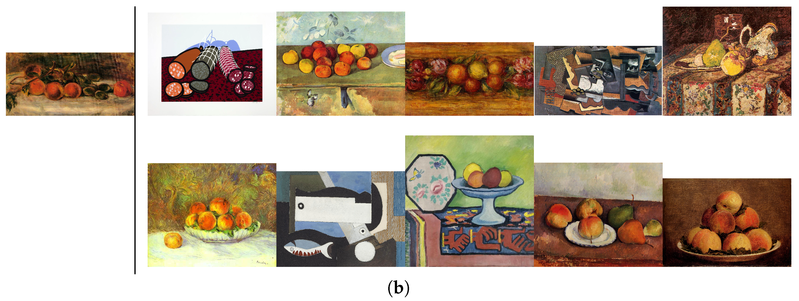
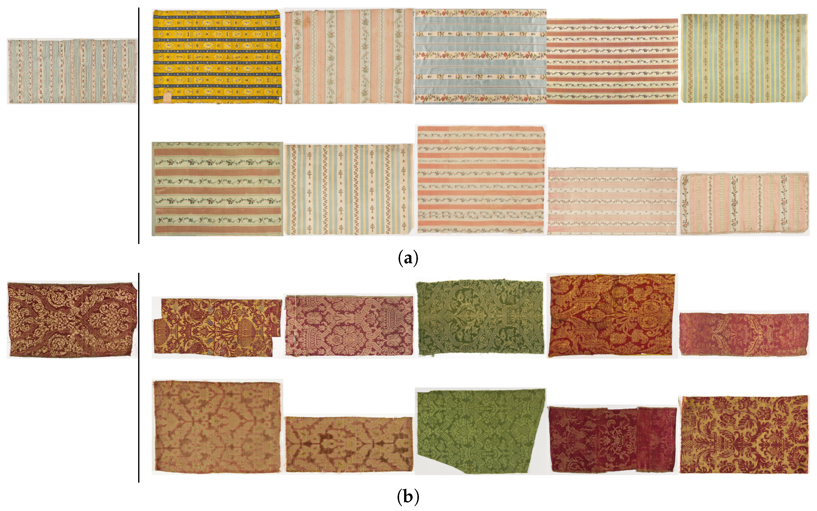
5.4. Qualitative Evaluation of the Results

In addition to the quantitative results presented in the previous sections, this section contains some qualitative results of the proposed image retrieval method for both datasets used in the evaluation. Examples for query images as well as the corresponding 10 most similar images retrieved by our method from the SILKNOW database are shown in Figure 5. Figure 6 shows two examples based on the WikiArt dataset. All of these examples result from the model variant sem + C, identified to be the best one in terms of the quantitative evaluation.

Even though exclusively semantic aspects of the depicted artifacts were considered in the training process, the results seem to be visually homogeneous. In the examples from the SILKNOW dataset (Figure 5), both the colors and the patterns of the query image and the retrieved images are predominantly similar. Figure 5a contains fabrics of a bright color with a stripe pattern, and Figure 5b shows fabrics in earth tones with fine-grained ornamental pattern. Similarly, the image retrieval examples from the WikiArt dataset mostly have colors matching those of the query images and show similar contents. Figure 6a contains images dominated by green and brown tones and depicts landscapes; Figure 6b shows mostly images of still-life images in red and brown. These examples also indicate that the semantics of a depicted artifact and its appearance is related to a certain degree.

6. Conclusions and Outlook

We have presented an approach for CNN-based descriptor learning in order to derive suitable image descriptors for silk image retrieval in the context of preserving European silk heritage. The training of the CNN considers both visual similarity concepts as well as semantic similarity concepts, where training data can be generated automatically by exploiting annotations related to the images in a digital collection. In this context, the annotations assigned to an image do not have to be complete to allow the image to contribute to training, which is of special interest given a real-world dataset. Besides similarity concepts that allow for the generation of training data without manual labeling, we proposed the integration of an auxiliary multi-task classification loss with the goal of supporting the clustering of the learned descriptors with respect to the characteristics of the depicted objects. Comprehensive experiments allow for an analysis of the impact of the individual loss components on the descriptors’ ability to reflect the similarity of a query image and the retrieved images in terms of the semantic annotations. In the experiments, k-NN-classification was conducted to allow for a quantitative evaluation without the need for a reference defining the optimal retrieval results for a set of test images or a known similarity status for each pair of images. The evaluation based on a dataset consisting of images of silk fabrics shows that utilizing the auxiliary classification loss during training indeed improves the performance by up to 3.3% in terms of the variable-specific overall accuracy and by up to 8.4% in terms of variable-specific F1 scores. It was observed that the largest improvements were achieved for variables with imbalanced class distributions. Further experiments on the WikiArt dataset showed the transferability of our approach to other digital collections, even though it was developed in the context of querying silk databases.

Future work could either focus on variations of the dataset to further investigate the transferability of the proposed method or to give hints for required modifications of the approach. As the presented descriptor learning approach relies on images with annotations indicating the classes of at least one semantic variable, it could theoretically be applied to any dataset or digital collection consisting of image and class labels of one or several variables. Thus, it would be interesting to analyze its behavior on other cultural heritage datasets, e.g., Art500k [17] or OmniArt [43], both consisting of images of artworks from different centuries, on other datasets related to fabrics, e.g., DeepFashion [67], consisting of images depicting clothes, and finally, on datasets showing images from a completely different domain, e.g., CelebA [68], consisting of face images with different face attributes. As far as the WikiArt data are concerned, additional hyperparameter tuning might improve the results beyond what could be shown in this paper.

From a methodological point of view, it would be interesting to investigate further auxiliary losses in order to improve the clustering behavior. This could include losses that directly address the clustering in descriptor space, such as the spherical loss or the center loss presented in [35]. Alternatively, a variation of the proposed self-similarity loss—e.g., the representation learning approach in [69]—could be investigated, which forces the descriptors to be invariant to different appearances of an object in an image. In contrast to the self-similarity loss presented in this paper, which directly forces the descriptors of two images of the same object to be similar, ref. [69] allows the network to learn a mapping between the descriptors. A further possibility would be to introduce not only further restrictions on the descriptors by formulating constraints in a loss function but to exploit further information about the depicted objects by considering descriptive texts assigned to images. Possible datasets to develop and test such approaches could either be generated from the SILKNOW knowledge graph [1], like the dataset in the present work, or other multi-modal datasets with both annotations for multiple semantic variables as well as descriptive texts; e.g., SemArt [70].

Furthermore, an evaluation with another focus of the results of the presented image retrieval method would be interesting. Such an evaluation could aim to obtain an impression of how visually similar the retrieved images are, which probably requires interactive assessment by domain experts. Another conceivable goal of a further evaluation could be to analyze the impact of the similarity losses on the image classification. Instead of handling the classification loss as an auxiliary loss, one or several similarity losses could be analyzed with respect to their ability to improve image classification, where the similarity losses would than function as auxiliary losses for image classification. A strong motivation for such experiments is our observation that the combination of descriptor learning and image classification during training improves the ability of the learned descriptors to represent semantic properties, primarily those of variables with many classes and imbalanced class structures at test time. In this context, it would be interesting to compare the utilization of auxiliary similarity losses with other strategies that aim to tackle class imbalance problems in image classification.

References

1. Alba Pagán, E.; Gaitán Salvatella, M.; Pitarch, M.D.; León Muñoz, A.; Moya Toledo, M.; Marin Ruiz, J.; Vitella, M.; Lo Cicero, G.; Rottensteiner, F.; Clermont, D.; et al. From silk to digital technologies: A gateway to new opportunities for creative industries, traditional crafts and designers. The SILKNOW case. Sustainability 2020, 12, 8279. [Google Scholar] [CrossRef]
2. Bentley, J. Multidimensional Binary Search Trees Used for Associative Searching. Commun. ACM 1975, 18, 509–517. [Google Scholar] [CrossRef]
3. Jain, A.K.; Vailaya, A. Image retrieval using color and shape. Pattern Recognit. 1996, 29, 1233–1244. [Google Scholar] [CrossRef]
4. Gudivada, V.N.; Raghavan, V.V. Content based image retrieval systems. Computer 1995, 28, 18–22. [Google Scholar] [CrossRef] [Green Version]
5. Yang, H.C.; Lee, C.H. Image semantics discovery from web pages for semantic-based image retrieval using self-organizing maps. Expert Syst. Appl. 2008, 34, 266–279. [Google Scholar] [CrossRef]
6. LeCun, Y.; Boser, B.; Denker, J.S.; Henderson, D.; Howard, R.E.; Hubbard, W.; Jackel, L.D. Backpropagation applied to handwritten ZIP code recognition. Neural Comput. 1989, 1, 541–551. [Google Scholar] [CrossRef]
7. Krizhevsky, A.; Sutskever, I.; Hinton, G.E. ImageNet classification with deep convolutional neural networks. Adv. Neural Inf. Process. Syst. 2012, 25, 1097–1105. [Google Scholar] [CrossRef]
8. Chopra, S.; Hadsell, R.; LeCun, Y. Learning a similarity metric discriminatively, with application to face verification. In Proceedings of the 2005 IEEE Computer Society Conference on Computer Vision and Pattern Recognition (CVPR’05), San Diego, CA, USA, 20–25 June 2005; Volume 1, pp. 539–546. [Google Scholar] [CrossRef]
9. Wang, J.; Song, Y.; Leung, T.; Rosenberg, C.; Wang, J.; Philbin, J.; Chen, B.; Wu, Y. Learning fine-grained image similarity with deep ranking. In Proceedings of the IEEE Conference on Computer Vision and Pattern Recognition (CVPR), Columbus, OH, USA, 23–28 June 2014; pp. 1386–1393. [Google Scholar] [CrossRef] [Green Version]
10. Qi, Y.; Song, Y.Z.; Zhang, H.; Liu, J. Sketch-based image retrieval via siamese convolutional neural network. In Proceedings of the 2016 IEEE International Conference on Image Processing (ICIP), Phoenix, AZ, USA, 25–28 September 2016; pp. 2460–2464. [Google Scholar] [CrossRef]
11. Cao, Y.; Long, M.; Liu, B.; Wang, J. Deep cauchy hashing for hamming space retrieval. In Proceedings of the IEEE Conference on Computer Vision and Pattern Recognition (CVPR), Salt Lake City, UT, USA, 18–23 June 2018; pp. 1229–1237. [Google Scholar] [CrossRef]
12. Zhao, F.; Huang, Y.; Wang, L.; Tan, T. Deep semantic ranking based hashing for multi-label image retrieval. In Proceedings of the IEEE Conference on Computer Vision and Pattern Recognition (CVPR), Boston, MA, USA, 7–12 June 2015; pp. 1556–1564. [Google Scholar] [CrossRef]
13. Wu, D.; Lin, Z.; Li, B.; Ye, M.; Wang, W. Deep supervised hashing for multi-label and large-scale image retrieval. In Proceedings of the 2017 ACM on International Conference on Multimedia Retrieval (ICMR’17), Bucharest, Romania, 6–9 June 2017; Association for Computing Machinery: New York, NY, USA, 2017; pp. 150–158. [Google Scholar] [CrossRef]
14. Zhang, Z.; Zou, Q.; Lin, Y.; Chen, L.; Wang, S. Improved deep hashing with soft pairwise similarity for multi-label image retrieval. IEEE Trans. Multimed. 2019, 22, 540–553. [Google Scholar] [CrossRef] [Green Version]
15. Gordo, A.; Larlus, D. Beyond Instance-Level Image Retrieval: Leveraging Captions to Learn a Global Visual Representation for Semantic Retrieval. In Proceedings of the IEEE Conference on Computer Vision and Pattern Recognition (CVPR), Honolulu, HI, USA, 21–26 July 2017; pp. 5272–5281. [Google Scholar] [CrossRef]
16. Kim, S.; Seo, M.; Laptev, I.; Cho, M.; Kwak, S. Deep Metric Learning Beyond Binary Supervision. In Proceedings of the IEEE/CVF Conference on Computer Vision and Pattern Recognition (CVPR), Long Beach, CA, USA, 15–20 June 2019; pp. 2283–2292. [Google Scholar] [CrossRef] [Green Version]
17. Mao, H.; Cheung, M.; She, J. Deepart: Learning joint representations of visual arts. In Proceedings of the 25th ACM International Conference on Multimedia, Mountain View, CA, USA, 23–27 October 2017; pp. 1183–1191. [Google Scholar] [CrossRef]
18. Stefanini, M.; Cornia, M.; Baraldi, L.; Corsini, M.; Cucchiara, R. Artpedia: A new visual-semantic dataset with visual and contextual sentences in the artistic domain. In International Conference on Image Analysis and Processing (ICIAP); Springer: Cham, Switzerland, 2019; pp. 729–740. [Google Scholar] [CrossRef] [Green Version]
19. Garcia, N.; Renoust, B.; Nakashima, Y. ContextNet: Representation and exploration for painting classification and retrieval in context. Int. J. Multimed. Inf. Retr. 2020, 9, 17–30. [Google Scholar] [CrossRef] [Green Version]
20. Clermont, D.; Dorozynski, M.; Wittich, D.; Rottensteiner, F. Assessing the semantic similarity of images of silk fabrics using convolutional neural network. In ISPRS Annals of the Photogrammetry, Remote Sensing and Spatial Information Sciences; Copernicus GmbH: Göttingen, Germany, 2020; Volume V-2, pp. 641–648. [Google Scholar] [CrossRef]
21. Schleider, T.; Troncy, R.; Ehrhart, T.; Dorozynski, M.; Rottensteiner, F.; Lozano, J.S.; Lo Cicero, G. Searching Silk Fabrics by Images Leveraging on Knowledge Graph and Domain Expert Rules. In Proceedings of the 3rd Workshop on Structuring and Understanding of Multimedia HeritAge Contents (SUMAC ’21), Association for Computing Machinery (ACM), Chengdu, China, 20 October 2021; pp. 41–49. [Google Scholar] [CrossRef]
22. Li, J.; Ng, W.W.; Tian, X.; Kwong, S.; Wang, H. Weighted multi-deep ranking supervised hashing for efficient image retrieval. Int. J. Mach. Learn. Cybern. 2020, 11, 883–897. [Google Scholar] [CrossRef]
23. Shen, C.; Zhou, C.; Jin, Z.; Chu, W.; Jiang, R.; Chen, Y.; Hua, X.S. Learning feature embedding with strong neural activations for fine-grained retrieval. In Proceedings of the on Thematic Workshops of ACM Multimedia, Mountain View, CA, USA, 23–27 October 2017; Association for Computing Machinery: New York, NY, USA, 2017; pp. 424–432. [Google Scholar] [CrossRef]
24. Jun, H.; Ko, B.; Kim, Y.; Kim, I.; Kim, J. Combination of multiple global descriptors for image retrieval. arXiv 2019, arXiv:1903.10663. [Google Scholar]
25. Schroff, F.; Kalenichenko, D.; Philbin, J. FaceNet: A unified embedding for face recognition and clustering. In Proceedings of the 2015 IEEE Conference on Computer Vision and Pattern Recognition (CVPR), Boston, MA, USA, 7–12 June 2015; pp. 815–823. [Google Scholar] [CrossRef] [Green Version]
26. Zhou, X.S.; Huang, T.S. Relevance feedback in image retrieval: A comprehensive review. Multimed. Syst. 2003, 8, 536–544. [Google Scholar] [CrossRef]
27. Chen, Z.; Wenyin, L.; Zhang, F.; Li, M.; Zhang, H. Web mining for web image retrieval. J. Am. Soc. Inf. Sci. Technol. 2001, 52, 831–839. [Google Scholar] [CrossRef]
28. Sharif Razavian, A.; Azizpour, H.; Sullivan, J.; Carlsson, S. CNN features off-the-shelf: An astounding baseline for recognition. In Proceedings of the IEEE Conference on Computer Vision and Pattern Recognition (CVPR) Workshops, Columbus, OH, USA, 23–28 June 2014; pp. 512–519. [Google Scholar] [CrossRef] [Green Version]
29. Bromley, J.; Bentz, J.W.; Bottou, L.; Guyon, I.; LeCun, Y.; Moore, C.; Säckinger, E.; Shah, R. Signature verification using a “siamese” time delay neural network. Int. J. Pattern Recognit. Artif. Intell. 1993, 7, 669–688. [Google Scholar] [CrossRef] [Green Version]
30. Dutta, A.; Akata, Z. Semantically Tied Paired Cycle Consistency for Zero-Shot Sketch-Based Image Retrieval. In Proceedings of the IEEE/CVF Conference on Computer Vision and Pattern Recognition (CVPR), Long Beach, CA, USA, 15–20 June 2019; pp. 5084–5093. [Google Scholar] [CrossRef] [Green Version]
31. Deng, Y.; Tang, F.; Dong, W.; Ma, C.; Huang, F.; Deussen, O.; Xu, C. Exploring the representativity of art paintings. IEEE Trans. Multimed. 2021, 23, 2794–2805. [Google Scholar] [CrossRef]
32. Efthymiou, A.; Rudinac, S.; Kackovic, M.; Worring, M.; Wijnberg, N. Graph Neural Networks for Knowledge Enhanced Visual Representation of Paintings. In Proceedings of the 29th ACM International Conference on Multimedia, Virtual Event, China, 20–24 October 2021; Association for Computing Machinery: New York, NY, USA, 2021; pp. 3710–3719. [Google Scholar] [CrossRef]
33. Hamreras, S.; Boucheham, B.; Molina-Cabello, M.A.; Benitez-Rochel, R.; Lopez-Rubio, E. Content based image retrieval by ensembles of deep learning object classifiers. Integr. Comput.-Aided Eng. 2020, 27, 317–331. [Google Scholar] [CrossRef]
34. Liu, F.; Wang, B.; Zhang, Q. Deep Learning of Pre-Classification for Fast Image Retrieval. In Proceedings of the 2018 International Conference on Algorithms, Computing and Artificial Intelligence; Association for Computing Machinery, Sanya, China, 21–23 December 2018; pp. 1–5. [Google Scholar] [CrossRef]
35. Lin, H.; Fu, Y.; Lu, P.; Gong, S.; Xue, X.; Jiang, Y.G. Tc-net for isbir: Triplet classification network for instance-level sketch based image retrieval. In Proceedings of the 27th ACM International Conference on Multimedia, Nice, France, 2–25 October 2019; Association for Computing Machinery: New York, NY, USA, 2019; pp. 1676–1684. [Google Scholar] [CrossRef]
36. Huang, J.; Feris, R.S.; Chen, Q.; Yan, S. Cross-Domain Image Retrieval With a Dual Attribute-Aware Ranking Network. In Proceedings of the IEEE International Conference on Computer Vision (ICCV), Santiago, Chile, 7–13 December 2015; pp. 1062–1070. [Google Scholar] [CrossRef] [Green Version]
37. Barz, B.; Denzler, J. Hierarchy-based image embeddings for semantic image retrieval. In Proceedings of the 2019 IEEE Winter Conference on Applications of Computer Vision (WACV), Waikoloa, HI, USA, 7–11 January 2019; pp. 638–647. [Google Scholar] [CrossRef] [Green Version]
38. Fellbaum, C. WordNet: Wiley online library. Encycl. Appl. Linguist. 1998, 7. [Google Scholar] [CrossRef]
39. Mensink, T.; Van Gemert, J. The rijksmuseum challenge: Museum-centered visual recognition. In Proceedings of the International Conference on Multimedia Retrieval (ICMR’14), Glasgow, UK, 1–4 April 2014; Association for Computing Machinery: New York, NY, USA, 2014; pp. 451–454. [Google Scholar] [CrossRef]
40. Tan, W.R.; Chan, C.S.; Aguirre, H.E.; Tanaka, K. Ceci n’est pas une pipe: A deep convolutional network for fine-art paintings classification. In Proceedings of the 2016 IEEE International Conference on Image Processing (ICIP), Phoenix, AZ, USA, 25–28 September 2016; pp. 3703–3707. [Google Scholar] [CrossRef]
41. Sur, D.; Blaine, E. Cross-Depiction Transfer Learning for Art Classification; Technical Report CS 231A and CS 231N; Stanford University: Stanford, CA, USA, 2017. [Google Scholar]
42. Belhi, A.; Bouras, A.; Foufou, S. Towards a hierarchical multitask classification framework for cultural heritage. In Proceedings of the 2018 IEEE/ACS 15th International Conference on Computer Systems and Applications (AICCSA), Aqaba, Jordan, 28 October–1 November 2018; pp. 1–7. [Google Scholar] [CrossRef]
43. Strezoski, G.; Worring, M. Omniart: Multi-task deep learning for artistic data analysis. arXiv 2017, arXiv:1708.00684. [Google Scholar]
44. Bianco, S.; Mazzini, D.; Napoletano, P.; Schettini, R. Multitask painting categorization by deep multibranch neural network. Expert Syst. Appl. 2019, 135, 90–101. [Google Scholar] [CrossRef] [Green Version]
45. Castellano, G.; Vessio, G. Deep learning approaches to pattern extraction and recognition in paintings and drawings: An overview. Neural Comput. Appl. 2021, 33, 12263–12282. [Google Scholar] [CrossRef]
46. Stalmann, K.; Wegener, D.; Doerr, M.; Hill, H.J.; Friesen, N. Semantic-based retrieval of cultural heritage multimedia objects. Int. J. Semant. Comput. 2012, 6, 315–327. [Google Scholar] [CrossRef]
47. Castellano, G.; Lella, E.; Vessio, G. Visual link retrieval and knowledge discovery in painting datasets. Multimed. Tools Appl. 2021, 80, 6599–6616. [Google Scholar] [CrossRef]
48. Jain, N.; Bartz, C.; Bredow, T.; Metzenthin, E.; Otholt, J.; Krestel, R. Semantic Analysis of Cultural Heritage Data: Aligning Paintings and Descriptions in Art-Historic Collections. In International Conference on Pattern Recognition (ICPR); Springer: Berlin/Heidelberg, Germany, 2021; pp. 517–530. [Google Scholar] [CrossRef]
49. Grover, A.; Leskovec, J. node2vec: Scalable feature learning for networks. In Proceedings of the 22nd ACM SIGKDD International Conference on Knowledge Discovery and Data Mining, San Francisco, CA, USA, 13–17 August 2016; pp. 855–864. [Google Scholar] [CrossRef] [Green Version]
50. Chen, Y.W.; Sobue, S.; Huang, X. KANSEI based clothing fabric image retrieval. In International Workshop on Computational Color Imaging; Springer: Berlin/Heidelberg, Germany, 2009; pp. 71–80. [Google Scholar] [CrossRef] [Green Version]
51. Corbiere, C.; Ben-Younes, H.; Rame, A.; Ollion, C. Leveraging Weakly Annotated Data for Fashion Image Retrieval and Label Prediction. In Proceedings of the IEEE International Conference on Computer Vision (ICCV) Workshops, Venice, Italy, 22–29 October 2017; pp. 2268–2274. [Google Scholar] [CrossRef] [Green Version]
52. D’Innocente, A.; Garg, N.; Zhang, Y.; Bazzani, L.; Donoser, M. Localized Triplet Loss for Fine-Grained Fashion Image Retrieval. In Proceedings of the IEEE/CVF Conference on Computer Vision and Pattern Recognition (CVPR) Workshops, Nashville, TN, USA, 19–25 June 2021; pp. 3910–3915. [Google Scholar] [CrossRef]
53. Deng, D.; Wang, R.; Wu, H.; He, H.; Li, Q.; Luo, X. Learning deep similarity models with focus ranking for fabric image retrieval. Image Vis. Comput. 2018, 70, 11–20. [Google Scholar] [CrossRef] [Green Version]
54. Xiang, J.; Zhang, N.; Pan, R.; Gao, W. Fabric image retrieval system using hierarchical search based on deep convolutional neural network. IEEE Access 2019, 7, 35405–35417. [Google Scholar] [CrossRef]
55. Dorozynski, M.; Clermont, D.; Rottensteiner, F. Multi-task deep learning with incomplete training samples for the image-based prediction of variables describing silk fabrics. In ISPRS Annals of the Photogrammetry, Remote Sensing and Spatial Information Sciences; Copernicus GmbH: Göttingen, Germany, 2019; Volume IV-2/W6, pp. 47–54. [Google Scholar] [CrossRef] [Green Version]
56. He, K.; Zhang, X.; Ren, S.; Sun, J. Identity mappings in deep residual networks. In Computer Vision—ECCV 2016; Springer: Cham, Switzerland, 2016; pp. 630–645. [Google Scholar] [CrossRef] [Green Version]
57. Nair, V.; Hinton, G.E. Rectified linear units improve restricted boltzmann machines. In Proceedings of the 27th International Conference on Machine Learning (ICML-10), Haifa, Israel, 21–24 June 2010; pp. 807–814. [Google Scholar]
58. Srivastava, N.; Hinton, G.; Krizhevsky, A.; Sutskever, I.; Salakhutdinov, R. Dropout: A simple way to prevent neural networks from overfitting. J. Mach. Learn. Res. 2014, 15, 1929–1958. [Google Scholar]
59. Bishop, C.M. Pattern Recognition and Machine Learning, 1st ed.; Springer: New York, NY, USA, 2006. [Google Scholar]
60. Russakovsky, O.; Deng, J.; Su, H.; Krause, J.; Satheesh, S.; Ma, S.; Huang, Z.; Karpathy, A.; Khosla, A.; Bernstein, M.; et al. ImageNet Large Scale Visual Recognition Challenge. Int. J. Comput. Vis. 2015, 115, 211–252. [Google Scholar] [CrossRef] [Green Version]
61. He, K.; Zhang, X.; Ren, S.; Sun, J. Delving deep into rectifiers: Surpassing human-level performance on imagenet classification. In Proceedings of the IEEE International Conference on Computer Vision (ICCV), Santiago, Chile, 7–13 December 2015; pp. 1026–1034. [Google Scholar] [CrossRef] [Green Version]
62. Yosinski, J.; Clune, J.; Bengio, Y.; Lipson, H. How transferable are features in deep neural networks? arXiv 2014, arXiv:1411.1792. [Google Scholar]
63. Kingma, D.P.; Ba, J. Adam: A method for stochastic optimization. arXiv 2015, arXiv:1412.6980. [Google Scholar]
64. Lin, T.Y.; Goyal, P.; Girshick, R.; He, K.; Dollár, P. Focal loss for dense object detection. In Proceedings of the IEEE International Conference on Computer Vision (ICCV), Venice, Italy, 22–29 October 2017; pp. 2999–3007. [Google Scholar] [CrossRef] [Green Version]
65. Liu, W.; Chen, L.; Chen, Y. Age Classification Using Convolutional Neural Networks with the Multi-class Focal Loss. IOP Conf. Ser. Mater. Sci. Eng. 2018, 428, 012043. [Google Scholar] [CrossRef]
66. IMATEX. Centre de Documentació i Museu Tèxtil, CMDT’s Textilteca Online. 2018. Available online: http://imatex.cdmt.cat (accessed on 14 February 2019).
67. Liu, Z.; Luo, P.; Qiu, S.; Wang, X.; Tang, X. Deepfashion: Powering robust clothes recognition and retrieval with rich annotations. In Proceedings of the IEEE Conference on Computer Vision and Pattern Recognition (CVPR), Las Vegas, NV, USA, 27–30 June 2016; pp. 1096–1104. [Google Scholar] [CrossRef]
68. Liu, Z.; Luo, P.; Wang, X.; Tang, X. Deep Learning Face Attributes in the Wild. In Proceedings of the IEEE International Conference on Computer Vision (ICCV), Santiago, Chile, 7–13 December 2015; pp. 3730–3738. [Google Scholar] [CrossRef] [Green Version]
69. Chen, X.; He, K. Exploring Simple Siamese Representation Learning. In Proceedings of the IEEE/CVF Conference on Computer Vision and Pattern Recognition (CVPR), Nashville, TN, USA, 20–25 June 2021; pp. 15750–15758. [Google Scholar] [CrossRef]
70. Garcia, N.; Vogiatzis, G. How to read paintings: Semantic art understanding with multi-modal retrieval. In Computer Vision—ECCV 2018 Workshops; Springer International Publishing: Berlin/Heidelberg, Germany, 2018; pp. 676–691. [Google Scholar] [CrossRef] [Green Version]
71. SILKNOW Knowledge Graph. https://doi.org/10.5281/zenodo.5743090 (accessed on 29 November 2021).
Figure 1. CNN architecture. The input is an RGB image x of 224 × 224 pixels that is passed to a ResNet152 [56] backbone, resulting in a 2048-dimensional feature vector f R N ( x ) . After a ReLU activation and a dropout layer, the feature vector is presented to N L j f c fully connected layers joint fc consisting of N N j f c nodes each and delivering the feature vector f j f c ( x ) . The head of the network consists of two branches: a classification head and an image retrieval head. The image retrieval head normalizes the vectors f j f c ( x ) to unit length, leading to the descriptors f ( x ) for image retrieval; it is used both in training and in testing. The classification head consists of N L f c- t m further fully connected layers f c - t m with ReLU, each consisting of N N f c- t m nodes. They map the joint representation f j f c ( x ) to task-specific representations and m classification layers f c - c m for multi-task classification with as many nodes as there are classes for the mth variable. The softmax activations y m k can be interpreted as posterior probabilities P ( C m k | x ) for the kth class of the mth variable. The broken line indicates that the classification head exists only at training time.
Ijgi 11 00082 g001
Figure 2. Examples for images in the SILKNOW dataset from the IMATEX collection. The five images have the following class labels (from left to right): timespan: unknown, 18th century, unknown, 19th century, unknown; place: IR, unknown, unknown, FR, unknown; material: metal thread, animal fibre, vegetal fibre, animal fibre, vegetal fibre; technique: unknown, damask, unknown, unknown, embroidery. © Museu Tèxtil de Terrassa/Quico Ortega [66].
Ijgi 11 00082 g002
Figure 3. Class structures and class distributions of the WikiArt dataset for the three variables genre (a), artist (b) and style (c). The blue bars indicate the number of images in the training set, the red bars correspond to the validation set, and the green bars correspond to the test set.
Ijgi 11 00082 g003
Figure 4. Examples for images in the WikiArt dataset. The five images have the following class labels (from left to right): artist: Rembrandt, Vincent van Gogh, Pierre Auguste Renoir, Pablo Picasso, Salvador Dali; genre: portrait, genre painting, landscape, still life, illustration; style: Baroque, Realism, Impressionism, Cubism, Abstract Expressionism.
Ijgi 11 00082 g004
Figure 5. Qualitative results of the experiment sem + C conducted on the SILKNOW dataset, where (a) and (b) each show one result. The first column shows the query image and the second column lists the corresponding ten most similar images according to our method, in ascending order by descriptor distance from top left to bottom right. © Museu Tèxtil de Terrassa/Quico Ortega [66].
Ijgi 11 00082 g005
Figure 6. Qualitative results of the experiment sem + C conducted on the WikiArt dataset, where (a) and (b) each show one result. The first column shows the query image and the second column lists the retrieved ten most similar images to the query image in ascending order by descriptor distance from top left to bottom right.
Ijgi 11 00082 g006aIjgi 11 00082 g006b