Commuter Mobility Patterns in Social Media: Correlating Twitter and LODES Data

Abstract

The Longitudinal Employer-Household Dynamics Origin-Destination Employment Statistics (LODES) are an important city planning resource in the USA. However, curating these statistics is resource-intensive, and their accuracy deteriorates when changes in population and urban structures lead to shifts in commuter patterns. Our study area is the San Francisco Bay area, and it has seen rapid population growth over the past years, which makes frequent updates to LODES or the availability of an appropriate substitute desirable. In this paper, we derive mobility flows from a set of over 40 million georeferenced tweets of the study area and compare them with LODES data. These tweets are publicly available and offer fine spatial and temporal resolution. Based on an exploratory analysis of the Twitter data, we pose research questions addressing different aspects of the integration of LODES and Twitter data. Furthermore, we develop methods for their comparative analysis on different spatial scales: at the county, census tract, census block, and individual street segment level. We thereby show that Twitter data can be used to approximate LODES on the county level and on the street segment level, but it also contains information about non-commuting-related regular travel. Leveraging Twitter’s high temporal resolution, we also show how factors like rush hour times and weekends impact mobility. We discuss the merits and shortcomings of the different methods for use in urban planning and close with directions for future research avenues.

1. Introduction

Historical land-use and development patterns, coupled with federal, state, and local policies have resulted in severe imbalances between jobs and housing in many sprawling metropolitan regions [1]. In most major American metropolitan areas, the results are apparent—rising housing costs, long commute times and bad traffic. The aim of transportation planning is to reduce the friction of distance, thereby increasing people’s mobility [2].

By focusing on work commutes rather than non-work trips, policymakers streamlined and simplified the complexities of travel behavior, although research has consistently acknowledged their importance and influence [3,4]. Much of what has been written about the journey to work appears to be based on conventional/traditional attitudes where the journey is characterized as a trip that occurs from a permanent residential location to a permanent work location. Transportation planning and policy developed in the 20th century struggles to keep up with the changing and dynamic nature of work in the 21st century, since statistics capturing human mobility are expensive to obtain and deteriorate quickly as existing mobility patterns change and new ones emerge [5,6]. The most detailed U.S. example of such statistics currently available are the Longitudinal Employer-Household Dynamics Origin-Destination Employment Statistics (LODES) [7], which are made available by the U.S. Census Bureau. The LODES data cover the entire U.S. and quantify commuter flows between census blocks. Because of their fine spatial granularity, high quality and coverage, they serve as an important tool to inform decision-making in regional and urban planning. One significant drawback of the LODES data is that they exclusively cover commuting traffic, which means that they do not cover trip types such as shopping or social activities. Yet, based on the survey data provided by the Federal Highway Administration (FHWA) [8], only a small portion, namely 16.6% of all trips, or 20.8% of vehicle miles, account for trips to or from work made with privately operated vehicles. Some regional transportation authorities have developed expensive yet sparse surveys trying to capture the mobility not covered by LODES, but they cover less than one percent of the population in the study area. Therefore, LODES data have been used as a surrogate for all forms of U.S. mobility. About 86% of Americans use a car to get around. In our study region, the San Francisco Bay Area, that number is approximately 76%, although this average is skewed by the only 41% commuters recorded in central San Francisco, while the rest of the region follows the national trend. Another outlier characteristic of San Francisco that we will explore when discussing our results is that some 50% of workers in the city work at home or commute short distances on foot or by bicycle [6].

For this study, we use geo-social network data (GSND) in the form of “tweets”, taken from the social media platform Twitter to derive mobility patterns, which we correlate with LODES data. They can be harvested in an automated fashion via the platform’s provided application programming interface [9]. Each of the tweets used in the study has a singular timestamp and position, thereby enabling us to aggregate the data temporally and spatially at any required scale. By counting the number of recurring connections between different regions, we derive weighted connectivity information. We refer to these weighted connections as Twitter flows throughout the remainder of the paper. The origin-destination (OD) data structure of the twitter flows is identical to that of the LODES data, which also represent flows. By partitioning and aggregating tweets, we can test how stable the association between Twitter flows and LODES is in different contexts. The finest available spatial granularity of LODES data is the census block level, which makes the census block level an appropriate aggregation level for the GSND to conduct direct comparisons. In the research presented in this paper, we address the following research questions:

• To what degree do commuter flow patterns identified in GSND correlate with official LODES commuting data?
• Which traffic flow information beyond commuting is contained in GSND?
• How strong is the influence of spatial scale on correlations between flows extracted from GSND and LODES commuting flows?

We compare Twitter and LODES flows with two different approaches to address the research questions. The first approach consists of an exploratory part, in which we show different spatiotemporal characteristics like changes in flow magnitudes and distribution over time and how the flows are affected by cyclical temporal phenomena like the time of day. Additionally, we integrate land-use data on the parcel-level into the analysis, to show the flow connectivity between pairs of land-use classes. For the second approach, we correlate OD data to assess how Twitter and LODES flows are associated. We do this comparison in a region-based approach on three spatial scales, as well as on the basis of individual street segments.

2. Related Work

Twitter and other GSND sources were used in a number of other studies pertaining to human mobility, for example in the detection and visualization of mobility patterns [10], events and traffic disruptions [11], and a range of other applications concerning urban planning and activity and mobility in general [12]. In one study carried out in the New York City area, researchers estimated mobility patterns and human activity on the county level based on Twitter data, concluding that the data is suitable for the purpose [13]. Similarly, Twitter data were shown to be suitable predictors of human mobility in a variety of urban settings. [14,15]. Depending on the use case, it can be useful to extract movement information in the form of OD matrices from GSND, as is the case in this study. One approach to do this is by regionalization of the GSND and then deriving trips from sequences of visited regions. These can then be aggregated to form an OD matrix [16]. The regionalization of tweets in this study works similar, although we utilize only those regions that contain a tweet cluster to skew the OD matrix towards regularly occurring trips.

The problems surrounding the identification of work-related activity and mobility in Twitter data have also been addressed using spatial autocorrelation and semantic text analysis methods in temporal bins [17].

The use of GSND as a new data source in urban planning is not limited to traditional study designs, however. The data’s high temporal resolution allows us to conduct studies on virtually any temporal scale [18]. This potential for high temporal resolution of mobility data is a factor that motivates this study, because if linked with other data, it would allow researchers to explore a myriad of temporally dependent effects, such as traffic volumes, traffic jams or accidents and the role that seasonality, daytime or weather conditions play in them.

For the interpretation of the study results, the temporal and spatial heterogeneous nature of the input data [19,20] should be taken into account. The temporal aspect is not only of linear nature, but has also cyclical aspects like daytime and day of the week to consider [21]. In this study, we address these effects through feature engineering prior to the temporal clustering process.

One research question posed above concerns the traffic not generated by commute trips. This number is largely unknown, because of the high costs to obtain relevant data. Aside from a small, municipality-based study [22] and a small national study [23], we identify only a few examples of related work in this topic area. In one instance, GSND in combination with a set of points of interest were used to develop a gravitation model for the city of Chicago [24]. A study conducted in New York City describes training a neural network model based on GSND for augmentation of a gravity model [25]. The aforementioned gravity model [26] also defines the principles based on which we derive flow data from GSND in this study.

GSND [27,28] have also been integrated with simulation models to determine travel demand [29]. One way to estimate travel demand and commuting patterns very similar to our approach is to derive them from geolocate tweets based on regularly visited locations [30]. The authors achieved similar results when using GSND to estimate official commuter numbers. However, they do not address non-commuter trips. We contribute to this body of knowledge by exploring the exchangeability between Twitter and LODES data. Another contribution to the work listed above are to highlight the importance of scale and the difference between OD and graph-based comparisons of the results.

3. Materials

3.1. Study Area Description

Our study area is located in the San Francisco Bay Area, shown in Figure 1. Over the past two decades, the region has seen rapid population growth. In 2020, it housed 7.75 million people, living in 101 municipalities. An estimate for the year 2040 predicts an additional 2.1 million inhabitants and 1.1 million jobs for the area [31]. The increasing demand in housing that follows this trend, in combination with the present regulatory and topographic constraints has led to land-use changes and aggravated traffic and environmental problems [32,33].

The nine counties that make up the area exhibit very different growth patterns. This, in combination with existing settlement patterns, has resulted in large discrepancies between the demand for housing and the availability of jobs [34]. Because the traffic system is constrained by the area’s topography necessitating bridge crossings, the resulting travel demand overloads the road system [35].

3.2. Data Description and Preprocessing

The LODES data are a product derived from employment statistics, surveys and administrative data. While most professions are covered in LODES, some of them, like military, security-related or self-employed are not represented. The data also only lists one OD pair per worker and employment site, which leads to a possible misrepresentation of work trips from people working at multiple locations. The quality of geographic information included in the data is not entirely consistent. While most workplaces and home locations are reported with sub-county precision, three percent of work locations and four percent of home locations are either reported on the county level or have no valid address. Further information about the LODES specifics is available in the supplementary materials [36]. The data are provided as text files that encode a sparse matrix in long-form format.

California has 710,485 census blocks. The corresponding LODES data list a total of 15,327,971 flows between blocks as home-work connections. The data also contain the number of jobs based in each individual block, totalling 16,566,140. LODES data contain no information about the modal split, though. Census data on the tract level [37], however, provides some insights into the means of transport. The LODES data contain a total of 3,252,286 individual commuter connections between 109,228 census blocks in the nine-county study area. Some of these connections occur between the same pair of census blocks and aggregating all LODES data results in 2,972,821 flows.

The raw twitter data consist of 44,812,476 tweets from the time between 8 October 2010 and 19 April 2020, all of which are geolocated in the study area. Among other attributes, they each contain one timestamp, the text of the tweet that was posted by the user as well as a point location in form of geographic coordinates. Figure 2 shows the temporal distribution of tweets. The high variance seen in the curves can be explained by changing user behavior, irregular sampling or changes in Twitter’s data sharing policy. Throughout the years, Twitter, Inc. (San Francisco, CA, USA) changed its data-sharing policy several times, which affects data availability. Up until 09/2012, only a very small fraction of tweets were available to us, making analysis prior to that date less reliable. Tweets are not only posted by human users, but also automatically generated by bots. However, our study design assumes that the tweets were written manually. We therefore removed a portion of the raw data based on content that appeared to be automatically generated, such as updates from weather stations or advertisements [38]. We implemented the filtering process by manually identifying Twitter users that generated tweets that consisted of highly repetitive advertisements, news articles or weather stations in a randomly selected subset and deleting all tweets generated by that user. We repeated this procedure iteratively until we did not identify any more offending tweets. Applying the criteria resulted in a total of 33,755,914 tweets that we ended up using in the study.

For clustering the data by their timestamps, we did not use the absolute values of the timestamps, but rather the time of day regardless of the tweet’s date. Conventional clustering methods do not account for the cyclical nature of timestamps, thus introducing a seemingly large gap between the far ends of the scale, in this case shortly before and after midnight. To mitigate this effect, we matched each timestamp t onto a two-dimensional space with the coordinates $x=sin\left(\right(2\pi t)/T)$ and $y=cos\left(\right(2\pi t)/T)$ with $T=24$ h before clustering.

The geometries associated with the tweets are given as point coordinates with latitude and longitude. To meet the assumptions of our spatial analysis methods, we projected the data onto a Cartesian coordinate system.

The geometries of the outline data of the counties, census tracts and census blocks we use throughout the study were taken from the website of the United States Census Bureau [39]. As a brief overview, selected characteristics of the outline geometries and contained twitter data are shown in

Table 1. Study area description.

	County	Census Tract	Census Block
Number of Regions	9	1584	109,228
Mean Area [km2]	2357.7	13.4	0.2
Median Area [km2]	2126.5	1.6	0.02
Standard Deviation Area [km2]	1028.9	69.0	2.1
CV Area	0.44	5.15	10.50
Mean Number of Tweets	3,750,657	21,310	352
Median Number of Tweets	3,013,390	15,503	54
Standard Deviation Number of Tweets	2,794,267	27,339	1863
CV Number of Tweets	0.75	1.28	5.29

. Both the numbers of tweets and the region sizes have higher variations in the smaller regions, as indicated by their standard deviations and coefficients of variation (CV).

An additional dimension of the flows, relating to research question 2, is the trip purpose. By combining parcel-level land-use data from Boundary Solutions [40] and census block outlines, we can understand what motivates particular trips. However, the geometries of the two data sets are not exact matches. A large number of census blocks contain more than one land-use parcel. To harmonize them, we assigned the land-use class to a census block that makes up the majority of its area.

We also performed experiments on the street network level, for which we required a road graph. We used the graph data provided by OpenStreetMap [41]. Data download and preprocessing operations were handled using the Python module OSMnx [42]. We used all data of drivable public streets within a radius of 250 km around the study area center. The reason for extending the data this way was to be able to capture results of the routing process even though they contain street segments from outside the original study area, which could easily occur close to the edges. We used the NetworkX [43] implementation of the well-known Dijkstra’s algorithm for routing, with edge weights that aim to represent car travel.

Apart from the aforementioned libraries, we used PostgreSQL [44] databases with PostGIS [45] for handling and analysing spatial data. For further processing and visualization, we used Python [46], R [47] and QGIS [48].

4. Methods

This section describes the methods used to carry out our research. The results produced through our workflow are then presented in Section 5. Figure 3 illustrates the overall methodological workflow of the research presented in this paper. On the top left, preprocessing and analysis steps transform raw Twitter and LODES data into two corresponding OD matrices. The box on the right describes the integration of street network and land-use data to produce intermediate outputs, that is, trip purpose datasets and flow graphs. At the bottom of the figure, these intermediate outputs and the OD are combined to produce the final correlations and visualizations, each marked up with which research questions they are answering.

4.1. Computing Trajectories and Flows in Twitter Data

4.1.1. Detecting Clusters of User Locations

The emphasis of our research is on modeling the flows of regularly occurring trips, omitting one-off visits to random locations. For this, we identify the locations that have been visited by the same user multiple times and at similar times of the day. Only the tweets that were posted by a user in one of their routinely visited locations are then used for calculating flows. We employ the DBSCAN clustering algorithm [49] to determine spatial and temporal clusters in each individual’s tweets and hence identify potential origins or destinations of regular occurring trips. The algorithm requires the specification of a minimum number of points per cluster ($minpts$) and a search radius ($ϵ$). Using the “elbows” method [50], we chose a temporal threshold of ${ϵ}_t=30$ min and specified a minimum of five points and a search radius of 100 m for the spatial dimension. After identifying the clustered individual tweets, the census block that contains the centroid of the tweets is identified as a regularly visited location of that user.

4.1.2. Identifying Individual User Trajectories

Based on a user’s list of routinely visited blocks, we can now determine their movements between them. If a user sends tweets from two different blocks within a three-hour time span, we consider the resulting connection between the blocks a trip. The three-hour maximum was chosen as it represents the maximum amount of time needed to move between the furthest ends of our study area. It also leaves some room for the assumption that a user might not send a tweet immediately after beginning or ending their trip. As we are aiming to identify regular occurring direct trips, we want to avoid longer time spans that may involve intermediate stops. We do not explicitly distinguish between origins and destinations other than identifying the sequence in which two locations are visited. Applying this logic, we identified 1,060,393 connections as trips between regularly visited census blocks.

4.1.3. Identifying Directed Flows at Different Scales

With the list of all trips, we can now create the sums of all movements between any two census blocks and label the non-zero elements of such an adjacency matrix as flows between regularly frequented locations. Structurally, the LODES and Twitter matrices are identical, which allows us to compare them with each other. An added advantage of this aggregation is that it hides individual-level data, allowing for compliance with best practices in privacy protection [51,52].

One of our research questions is to see whether different temporal partitions of the Twitter may be used to identify non-commute trips and distinguish them from the commutes that are captured by the LODES data. In addition, planners would benefit from learning about fluctuations over time. For longer term trend analyses, the data was split into two-year chunks, which also helped to deal with the large variations in georeferenced Twitter data. The population of commute trips can be associated with flow data during typical rush hour times (6:00–8:00 a.m. or 3:00–5:00 p.m.) in the Bay Area. For this particular region, the rush hour times are relatively early in the day, because many companies have adjusted their business hours to be in sync with their business partners on the U.S. East Coast. We also selected subsets of the data based on whether they were produced during or outside of the weekend to capture differences in the resulting mobility behavior.

We also aggregated the flow data into higher-level census area units to determine the robustness of Twitter data at different spatial scales. The U.S. Census Bureau’s spatial hierarchy is a perfect tessellation of $censusblock\subset censustract\subset county$.

4.2. Flows between Spatial Regions and Land-Use Classes

We saw in the previous sub-section that structurally and functionally, the adjacency matrices of both the LODES and the Twitter data are identical, which allows us to compare every single OD pair and to quantify the differences. Since not every commuter tweets during their commute, the absolute number of flows between census blocks is much smaller and must be scaled proportionally to match the LODES data. Our comparison is based on correlation coefficients. Each datum of the LODES and Twitter OD pairs represents aggregated movement between a pair of census blocks. We compare these LODES pairs with the Twitter flow data and quantify differences between the two datasets. This comparison is possible, because even though the LODES and Twitter data are from different sources, they contain some shared information between them. We use the nonparametric Spearman’s rank correlation coefficient $\rho$. As we aggregated the data also to census tracts and counties, we ran the calculations at all three spatial scales.

Another way to distinguish commuter trips from other regularly occurring flows is to look at the land use of flow destinations. After aggregating parcel-level land use data to the census block level (and subsequently tract and county level) we can compare the OD pairs of the two adjacency matrices by their destination land use, which opens another avenue to distinguish the two statistical populations.

Given that LODES data by definition only contain work trips, whereas the Twitter data has no such constraints, we can use both the temporal as well as the land use dimension to conclusively identify differences between the two datasets. Commute and non-commute trips are, of course, not mutually exclusive, and we may expect to have both during rush hour times, just as we may observe commute destinations to lie in census blocks that in their majority (but not exclusively) have been classified as less likely to accommodate employment locations. But it would be fair to assume that commute trips will dominate rush hour times and destination land uses such as offices, commercial, or industrial. We employ Sankey diagrams visualizing land-use class connections to illustrate the flow magnitudes between land-use classes for both data sources. This follows similar uses of this technique for the visualization of land cover dynamics [53].

4.3. Mapping Flows to Street Segments

With the exception of the city of San Francisco, most commuters in the study area are travelling by car [6]. This is why we have mapped the travel paths for our OD pairs onto a street network weighted for car usage. For routing between pairs of census blocks, we chose the graph’s node closest to the centroid of each block. The routing routine returns a set of street segments used by each OD pair that multiplied by the number of trips for each pair gives us the total demand on each street segment exerted by both the LODES and Twitter flow data allowing for direct comparisons between the two data sets on an edge-by-edge basis. We used standard scores to account for the differences in flow volumes.

To inform the choice of comparison measure, we then calculated the correlation between the segment loads of the LODES and Twitter flows as shown in Figure 4. At the scale of the whole study area, and incorporating all Twitter-derived trajectories with the LODES-based ones, we could not find any statistically discernible difference between the two datasets (the correlation rates are perfect beyond the highest Z scores).

Given that Twitter and LODES flows should represent different aspects of mobility, such a high correlation rate is suspicious, and we chose to apply a spatial regression on the two data sets. This required to translate from a graph into an irregularly distributed point structure, taking the midpoints of over 3.1 million street segments (median length: 92 m) and assigning them the values of their respective travel demand. As we know how each original trip contributes to the street segment use, we could calculate the total demand for each of our temporal partitions of the Twitter data.

4.3.1. Correlating Twitter Flows and Lodes Flows

The incredibly high correlation between the approximately 3 million LODES trips and the approximately 1 million Twitter-derived trips can be ascribed to the law of large numbers: the two samples are drawn mainly from the same population, the Bay Area residents. Given sufficiently large sample sizes, the two samples are going to resemble each other more and more. This suggests that a comparison of the LODES data on one hand and different temporal partitions of the Twitter data on the other is more meaningful. We therefore investigated the relationships between different subsets of the Twitter data as well as between those and the LODES data with the goal to see whether the Twitter data may be used to provide short-term updates of the LODES data that may represent behavior changes.

Table 2. Comparison of the comprehensiveness of the datasets used in this study. The features are the street segments of the OSM network for the study area.

Layer	Feature Count
Total OSM network	541,898
LODES	136,492
All Twitter	114,002
Twitter—Outside of rush hour	112,769
Twitter—Weekends	97,997
Twitter—Rush hour	96,896
Twitter—Outside of rush hour 2018/19 only	38,330
Twitter—Weekends 2018/19 only	31,766
Twitter—Rush hour 2018/19 only	31,441

provides an overview of the number of street segment that form the basis of the comparison.

We then ran spatial regression models on all the possible combinations of the entries in Table 2. Judging by their $r^2$ values shown in

Table 3. Explanatory power of different Twitter data subsets predicting LODES street segment loads.

LODES Prediction	Spatial Lag	Spatial Error
All Twitter	0.76117	0.766143
Twitter—Outside of rush hour	0.764129	0.770077
Twitter—Rush hour	0.728379	0.736184
Twitter—Weekends	0.763587	0.772134
Twitter—Outside of rush hour 2018/19 only	0.352977	0.425247
Twitter—Rush hour 2018/19 only	0.266606	0.320049
Twitter—Weekends 2018/19 only	0.349353	0.41174

and

Table 4. Explanatory power of subsets from the 2018/19 Twitter data predicting Twitter street segment loads for the entire study period.

All-Twitter Predictions 2018/19	Spatial Lag	Spatial Error
Twitter—Outside of rush hour	0.505801	0.602277
Twitter—Rush hour	0.418713	0.492426
Twitter—Weekends	0.515357	0.609862

, the spatial error model performs slightly better than the spatial lag model [54,55].

The results allow for the following conclusions. The two-year temporal subsets are insufficient to replace LODES-based street segment use but are indicative for overall Twitter-based street segment usage. This is a first evidence that the Twitter data does indeed represent different populations than the LODES data.

4.3.2. Determining Non-Work-Related Twitter-Derived Street Segment Usage

Another way to identify different trip types is to incorporate trip purpose. The safest (but also most difficult) way to do this is to semantically analyze a tweet’s content [17]. Here, we rely instead on the more indirect but complete co-variables of land use type as well as known point of interest at the trip destination and the time of day and day of week to derive trip purposes. The street segment assignment described in the previous section serves now for the creation of maps such as the ones shown in Figure 5. Map (a) shows where within the study area the detailed maps (b) and (c) depicting non-commute trips are located. The green lines in map (b) represent road segments usage on weekends, while the red lines in map (c) show road segments that are used on weekdays but outside of rush-hours. In addition to the expected differences in travel patterns, the two maps also match the trip purposes derived from the analysis of destination land-uses (e.g., short residential-to-residential trips during weekday non-rush hours and shopping and restaurant destinations on weekends.

5. Results

5.1. Flows between Spatial Regions and Land-Use Classes

Exploratory data analyses provide an overview of the region-based differences between Twitter and LODES data.

Table 5. Number of connections within and between regions by aggregation level and data source. The percentages indicate the relative share of connections for a given data source and aggregation level.

	Within Region		Across Regions
	Twitter	LODES	Twitter	LODES
Census Block	0 (0%)	4313 (0.1%)	946,907 (100%)	3,248,031 (99.9%)
Census Tract	404,121 (42.7%)	110,630 (3.4%)	542,786 (57.3%)	3,141,714 (96.6%)
County	833,318 (88.0%)	1,897,982 (58.4%)	113,589 (12.0%)	1,354,362 (41.6%)

shows a comparison of inter- and intraregional Twitter and LODES flows, so the number of flows that occur within a given spatial region versus the flows that occur between regions. Note that the number of Twitter flows within a block is zero by definition because we only count movement that happens between two distinct census blocks.

At a purely descriptive level, there are some notable differences between the LODES and the Twitter data. The vast majority of Twitter flows happen within their census tract and county, whereas over 40% of LODES connections cross county borders. The difference is particularly strong at the census tract level, where 42.7% of Twitter flows happen within a tract, whereas the same is true for only 3.4% of the LODES flows. This corresponds with the descriptive statistics of trip lengths and estimated car travel times given in

Table 6. Trip lengths on the OSM network.

	LODES	Twitter
Minimum	0.001 km/0 min	0.008 km/0 min
Median	12.660 km/14 min	2.800 km/3 min
Mean	22.538 km/19 min	7.561 km/6 min
Maximum	259.761 km/178 min	366.315 km/264 min

.

In addition to the inter- and intraregional comparisons of Twitter and LODES flows, we calculated Spearman’s rank correlation coefficient $\rho$ of flow magnitudes between regions for the three spatial scale levels and partitioned temporally. The results are shown in Figure 6. The scale dependence of correlations is salient, the comparison of smaller aggregation levels consistently results in lower correlation coefficients. The results during and outside of rush hours are very similar, although the correlations are a bit higher during rush hours.

Figure 7 is a county-level analysis of Twitter flows during rush hours (a), weekday Twitter flows outside of rush hours (b), and LODES data (c). The color-coded arrows of this chord diagram visualize both the direction and magnitude of flow between any of the nine counties. The numbers of connections show the higher absolute flow magnitudes of the LODES data. In addition, there are a lot more inter-county LODES connections than for the Twitter flows. For example, around half of the outgoing connections of Alameda County connect to other counties in the LODES data, whereas only about 15% of Twitter connections are outbound. The chord diagrams also highlight the exceptional nature of San Francisco, where the Twitter flows are a lot stronger compared to other counties.

The Sankey diagrams of Figure 8 show the connections between land-use classes for Twitter flows during rush hours (a), outside of rush hours (b) and LODES data (c). Compared to (c), the two Twitter flow diagrams appear at first glance to be quite similar, yet there are noteworthy differences between them. As we hypothesized before, there are fewer connections between residential areas during rush hour and this particular time span is dominated by connections between residential areas and work-related land-use classes. The distribution of land use classes for Twitter flow origin and destination areas compared to those of the LODES data is another indication for the clear separation of home and work location in the latter; something that cannot be expected of the Twitter data, which represent a wider functional range of trips.

5.1.1. Comparing Lodes with Twitter-Derived Street Segment Usage

A surprising result of the spatial error model in Table 3 is that rush hour trips are a poorer predictor of LODES trips than the ones outside of rush hour and during the weekends. This can be explained by the fact that actual work-related trips are less likely to be accompanied by tweets than non-commuting trips. The fact that a significant number of Twitter flows have residential origins and destinations is supportive of this notion and compares well with the results of national surveys of the FHWA. We already observed the relatively poor predictive capacity of the two-year subsets but would like to add here that relaxing the stringent individual road segment-based constraint might improve the results. We endeavor to continue our studies towards determining the appropriate scale thresholds for such predictions.

Approaching the question of whether the finer temporal resolution of the Twitter data could be used to update existing US Census datasets, we compared the 2018/19 subset to the much more voluminous Twitter data from previous years, again using spatial regression models. With the exception of rush trips, the results in

Table 7. Robustness of a two-year subset of Twitter data predicting LODES street segment usage.

Temporal Subset	${\mathit{r}}^2$
Twitter—Weekends	0.6098
Twitter—Outside of rush hour	0.6023
Twitter—Rush hour	0.4924

give us some satisfactory correlations.

5.1.2. Determining Rush Hour Twitter-Derived Street Segment Usage

As reported above, our goal to use rush hour Twitter data to predict the commutes provided by LODES proved to be elusive. The assumption that movement data from similar times of day should be similar in nature is contradicted by both the high number of residential-to-residential trips as well as by the significant differences in trip lengths. We now hypothesize that tweets before or after a trip to work are relatively rare and that the movements we observe during rush hour actually represent non-work trips—in spite of the time of day.

5.1.3. Determining Non-Work-Related Twitter-Derived Street Segment Usage

The main insight gained from the map in Figure 9, which depicts trips not captured by the traditionally used LODES data, is that people who tweet are first and foremost people who move about like everybody else. The attempt to discern differences between LODES-based movements and those derived from weekend Twitter data results in a maximum correlation of $-0.13$—a truly small difference. In addition, the areas of difference show no spatial autocorrelation, which means that they are randomly distributed. Most of these small differences occur in residential areas (with a few others in remote areas) and none match known points of interest, such as shopping centers or sports venues. To the contrary, for well-known traffic chokepoints, the street segment loads confirm what we know from the LODES data. Complementing our insights from the rush hour data and the national surveys of the FHWA, the ubiquity of the flows derived from our Twitter data points to its potential as a new source of information about trips outside the commute realm that has hitherto not been available. In this context, it is important, however, to remind the reader that the way we selected the Twitter data purposefully excludes trips that do not show up repeatedly for the same individual and hence underestimates the amount of non-routine trips.

6. Discussion and Limitations

6.1. Discussion of Research Questions

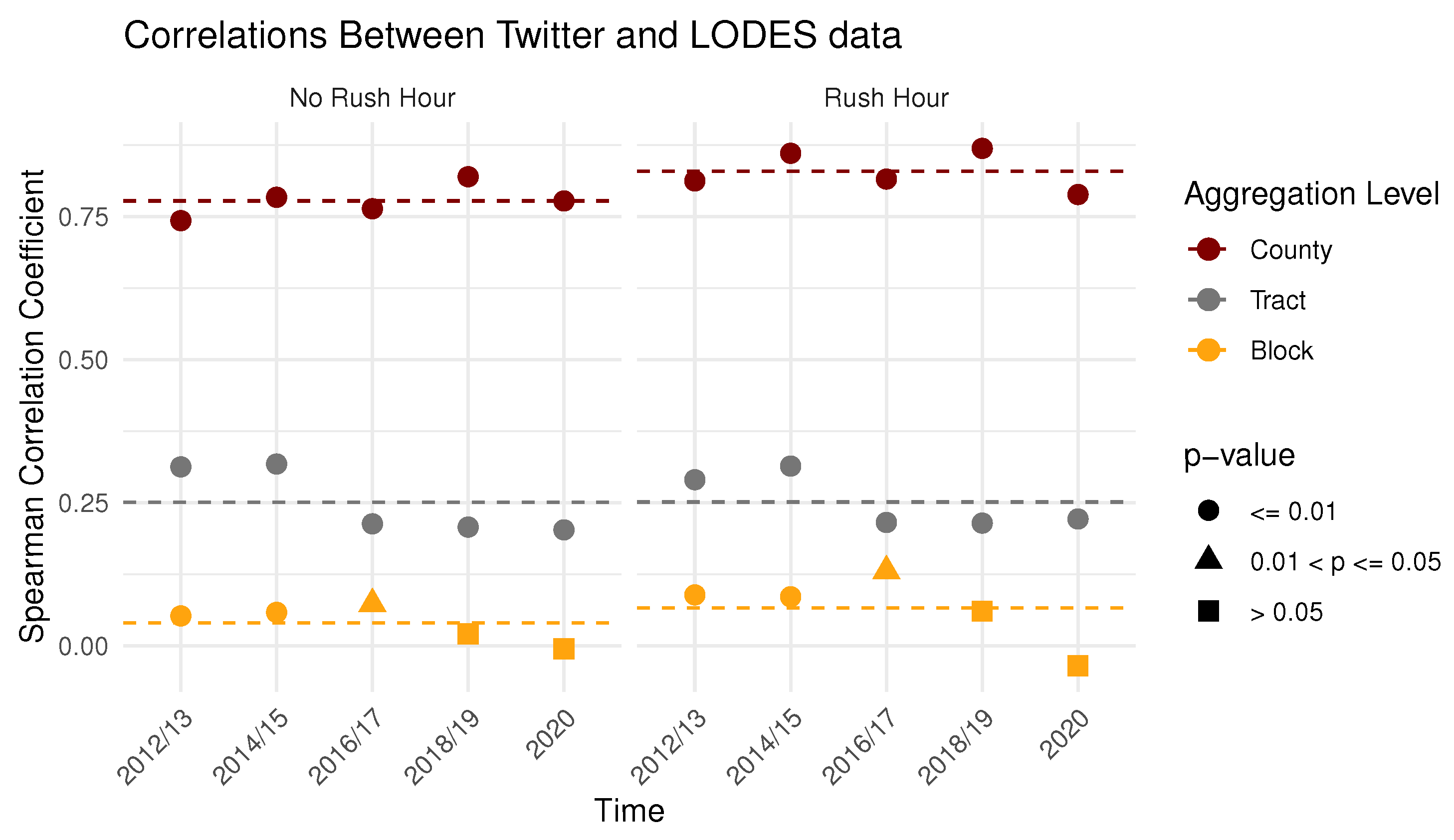
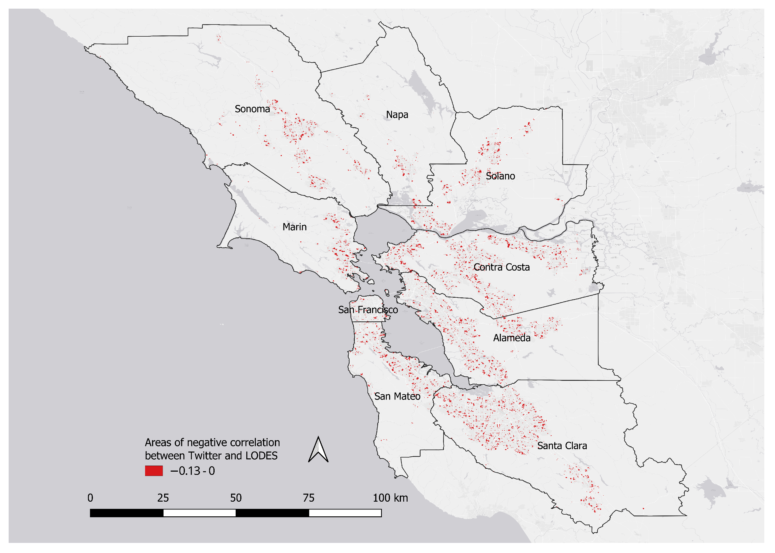
To address research question 1, to what degree do commuter flow patterns identified in GSND correlate with official LODES commuting data, we analyzed the correlations among the OD pairs of both data sources at multiple spatial scales. As confirmed by other county-level analyses of Twitter-based flow data, we found that there is a strong correlation at smaller spatial scales. In contrast, when we mapped the flows at highly localized to the street segment levels, we found indications that a large portion of Twitter flows are different from direct work trips. They tend to be significantly shorter, even if they occur during rush hour times.

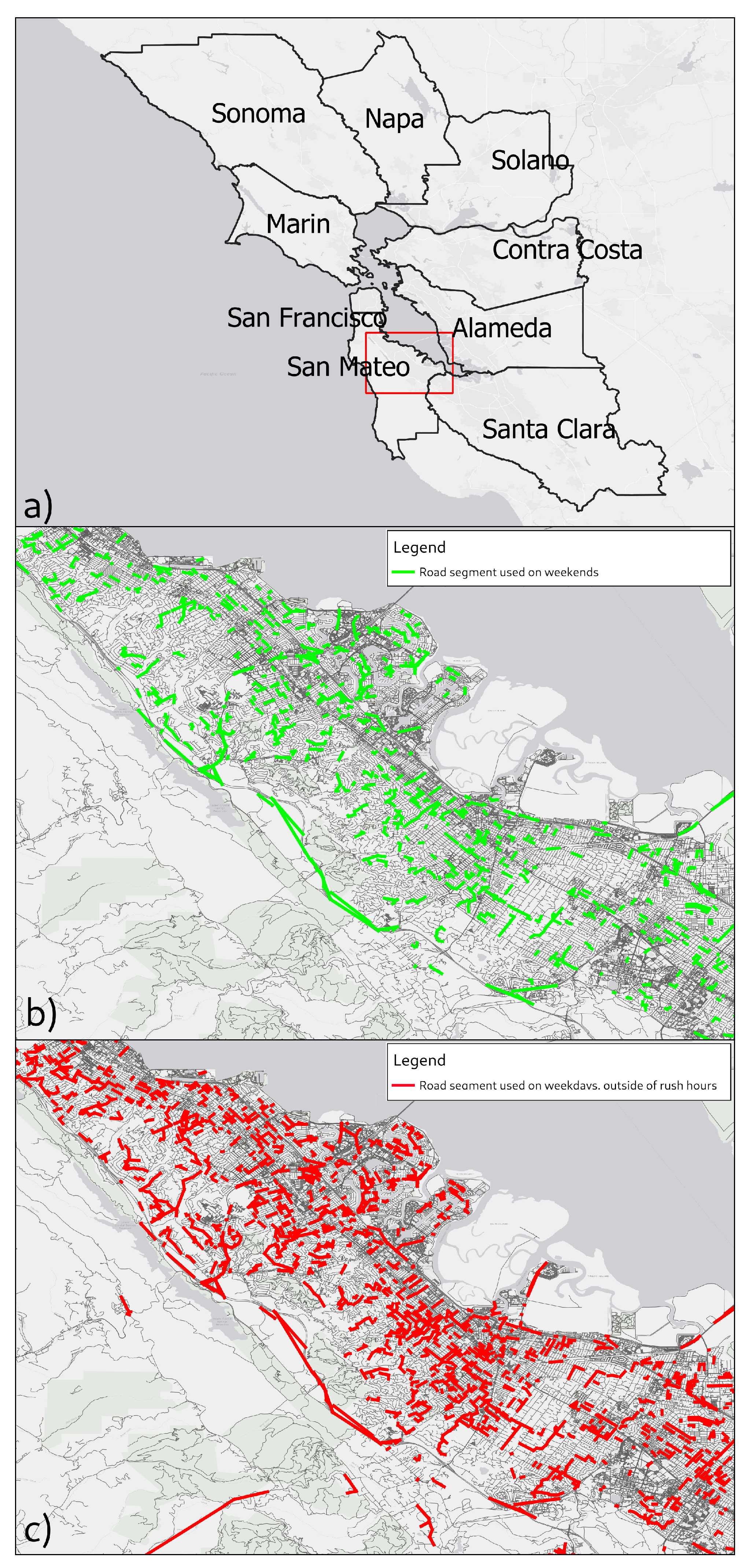
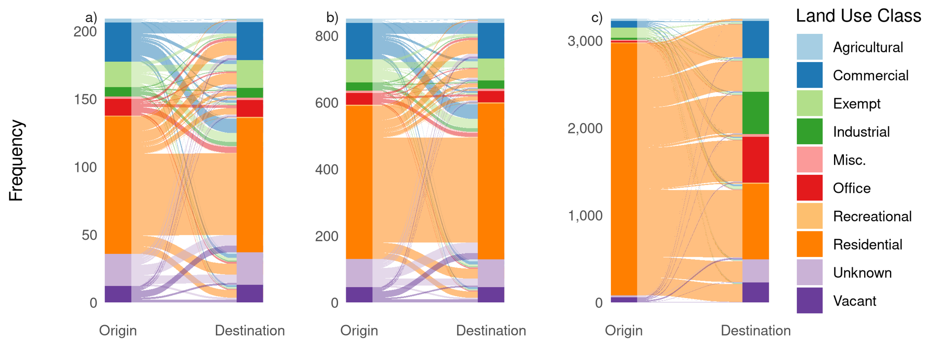
To address research question 2, which traffic flow information beyond commuting is contained in GSND, we used both destination land use classes as well as time stamps outside of typical rush hours to derive different trip populations. Both methods lead to clearly distinguishable movement patterns. Our assumption that LODES trips show a stronger linkage between residential and work-related land uses than non-commuter movements is confirmed by the comparison of parts (a) and (b) in the Sankey diagrams of Figure 8.

To address research question 3, how strong is the influence of spatial scale on correlations between flows extracted from GSND and LODES commuting flows, we again refer to the correlation coefficients of Twitter and LODES flows at different times and on different spatial scales. The correlation coefficients show that for county-level mobility, Twitter and LODES exhibit robust, high correlations. This is consistent with a number of nation-wide, county-level resolution studies.

6.2. Discussion of Methods

For the purpose of this study, we focused on movements within our study area that a user visits repeatedly. We implemented this premise by only including fine-grained areas (no bigger than a census block) in which we detected spatiotemporal clusters of tweets by a given user. We implemented this constraint to ascertain that we capture routine travel behavior, which means that rarely visited locations have purposefully been excluded from this analysis. A built-in assumption here is that frequent visits to a location result in frequent tweets. This is a limitation that is not borne out of any particular conceptual model but based in the nature of the data. Another limitation of our work is that trip chains between home and work, in which the user makes regular stops at intermediate locations can be picked up as regularly occurring trips that skew the Twitter OD data away from the LODES data. This effect can also be beneficial, however, if the actual road use patterns created by commuters are of interest.

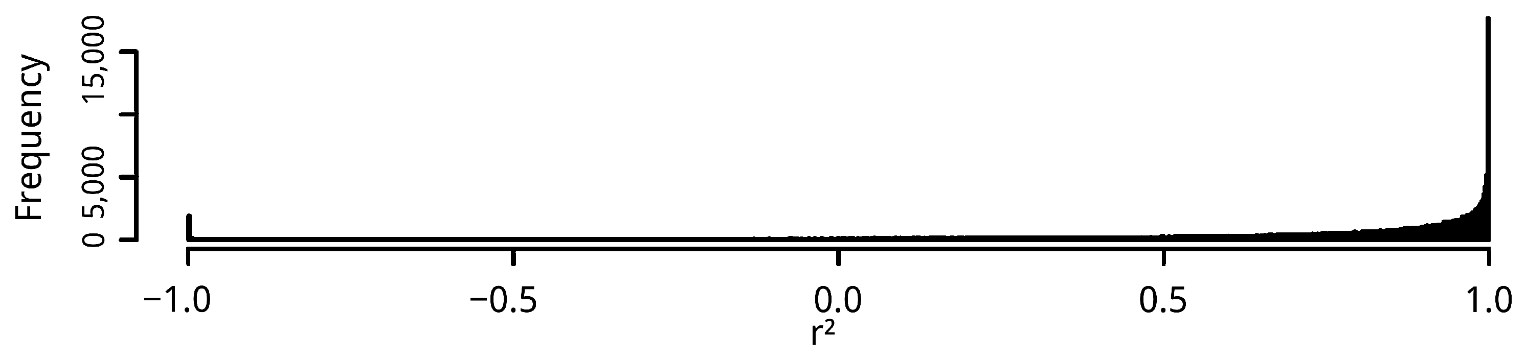
For our area-based approaches, we emphasize flow magnitudes, as well as the origin and destination areas. The direct comparisons of correlation coefficients result in simple summary statistics, which are compact and easy to compare, but do not provide deeper insights into the spatial characteristics of the results. This is compounded by the inherently binary nature of OD pair comparisons: Two OD pairs are either identical or they are not. This distorts the reality that each OD pair is a simplified representation of what is actually a route along a street network. Two OD pairs with starting or end points in close spatial proximity but in different area units, are likely to share some street segments in their routes. However, they are not identical and are therefore, a mismatch from an area-based perspective. This skews the correlation statistics towards low values, especially for smaller areas. The graph-based reasoning methods are better suited to capture such spatially similar but non-identical connections. This effect can be observed when comparing the region-based results in Figure 6 with the graph-based ones from Table 3. Although the median street segment length of $92m$ constitute a finer scale than the census block level, the predictive power is significantly higher. It is worth noting, however, that using a least-cost path algorithm to derive road segment usage from OD pairs assumes highly efficient travelling behavior, which might not be given.

Aside from road graphs, the finest area unit for direct comparisons of LODES and Twitter data used in this study is the census block. Georeferenced Twitter data typically derive their location from a mobile device’s Global Positioning System (GPS) sensor. Using GPS locations would potentially allow comparisons on an even finer spatial scale, however this would also require appropriate reference data. In the case of this study, we chose the census block scale of the LODES data as the limit.

A significant portion of the land-use class connections are residential to residential trips. This is not a surprising result for the Twitter flows, since we expected movement between different private residences as part of day-to-day social interactions. In the LODES data, however, this was unexpected, since we did not expect many residential areas to function as workplaces. We identified possible reasons for this discrepancy. Areas classified as residential areas in our land-use data could in fact be compound areas of different land-use classes. Also, by integrating the land-use data on the census block level, compound areas could have been aggregated to the most dominant land-use class, thereby obscuring some commercial land-use class parcels. A possible alternative would be to use a weighted approach to account for such areas.

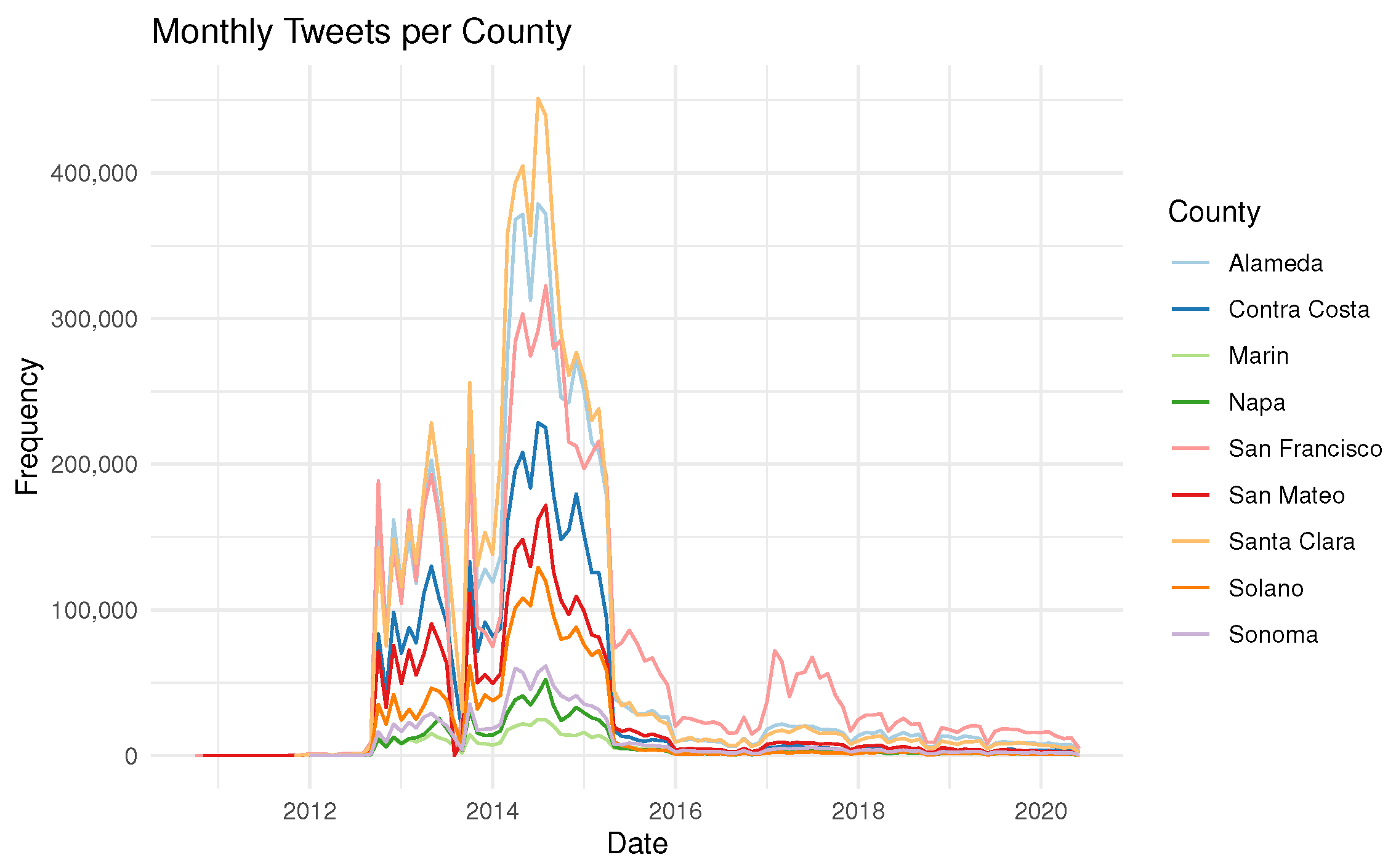
Twitter usage is skewed by demographic and geographic context. The population of some regions and the movements of their members will be represented more strongly than others. There might, for example, be residential areas with few active Twitter users, but a large working population. Or there might be places with few permanent residents that attract large numbers of visitors like sports venues or shopping centers. It is important to incorporate knowledge of such places when interpreting the results of a study like ours. Another factor that influences the availability of georeferenced Twitter data is time. There can be multiple reasons for changes in data availability over time, for example changes in user numbers, data sharing policies by Twitter or differences in user activity over time. To ensure that the results of the study still hold despite these changes, it is important to validate temporal subsets of the data to ensure their integrity.

While LODES is limited to home-to-work mobility, Twitter flows represent other travel purposes as well. Ideally, the difference between the two datasets should be based on non-commuting mobility only. In reality, however, there is some overlap between commuting and non-commuting trips during rush hours and there is also a not insignificant number of commute trips outside of traditional rush hours, which make it hard to separate the movement populations.

From the perspective of statistical error analysis, it is possible to scale the Twitter origin land-use class distributions to resemble the distributions from LODES and adjust the Twitter destination land-use classes accordingly. This would skew the distribution of Twitter flows towards that of LODES at the cost of introducing an additional error term. Another issue regarding the use of LODES data as reference for Twitter flows is the temporal lag between the two data sources. The LODES data used in this study are from 2019 and therefore more recent than most of the Twitter data. Discerning the effects of this lag on results is problematic, because the amount of Twitter data, user demographics and data availability may also vary over time. Results with high temporal lags must therefore be interpreted carefully and, where possible, substantiated with additional data.

LODES data do not contain information about temporal trip characteristics like the time of day or weekday. Having this additional information would be beneficial for the quality of time-sensitive analysis and for specifying assumptions about the commuting process.

Movement data of a person may reveal intimate insights into their life. Following the geo-privacy by design guidelines by [51,52], we apply the principle of data economy throughout the entire workflow and only disclose results where the spatial and temporal aggregation prevents the identification of individuals. It is therefore crucial, that researchers utilizing similar methods and data sources uphold the principles of information privacy and ideally, develop methods that obscure personal information in GSND adequately without compromising study outcomes.

6.3. Discussion of Results and Relevance for Urban Planning

Our comparison of the two differently sourced flow data employed methods designed to highlight different aspects of the data. Focusing on flow magnitudes, we found spatial scale to be the most influential factor. At small scales such as the county level, we are able to model the proportion of flows well, whereas on larger scales, we observe significant differences between Twitter and LODES flows. Given the observed differences between three spatial scales, we recommend investigating even more scale levels to learn more about this aspect of the data. Alternatively, one could abandon the use of administrative boundaries altogether and use regularly spaced grid cells to explore the impact of spatial scales.

The transition to a road network analysis with its comparison of street segment loads allowed us to compare different flow populations with much higher granularity. We found that during rush hours, the data sources deviate significantly, which suggests that Twitter flows capture regular trips with purposes other than commuting. The graph-based analysis also shows that Twitter trips are generally much shorter than LODES commutes, which lends support to trip purposes other than direct travel to work as well, even if many of them fall into rush hour times. This interpretation is also supported by the analysis of land use class connections, which again show significant differences between LODES and Twitter. One assumption that is built into the model based on the street network is that the mode of transport is by car, which is implemented via the graph weighting scheme. This skews the results towards car-specific infrastructure like highways, which has to be considered when interpreting them. As one would expect from trips to work, LODES data contain fewer connections between residential areas when compared to Twitter flows. Finally, the proportions of the remaining land use classes point again to differences in trip purpose.

Potential Use in Urban Planning

Transportation planning and policy requires long-range planning that uses demographic forecasting and travel demand modeling to direct infrastructure investments. The existing data sources like the decennial census and its derivative data products such as LODES are well suited to support these analyses. In recent years, the prevalence of volunteered geographic information and similar data sources made available by commercial providers like SeeClickFix [56], Waze [57], or, in the case of this study, Twitter, have helped planners and managers undertake just-in-time planning, making adjustments in response to public requests for intervention. We argue that GSND from Twitter can be used to support planning in the three to five-year time frame, to undertake modest capital improvements and other planning and policy interventions that are likely to benefit the public because the data are reliable and immediately usable to planners. Given that Twitter data availability varies significantly over time and the volume declined toward the end of the study period, alternative, more stable data sources of comparable data structure would be beneficial when using these methods in urban planning.

Given that only 16.6% of vehicle trips on U.S. streets are work-related [8], the remaining 83.4% of trips are not addressed by the LODES data. As we could show in our large-scale, region-based comparisons, Twitter-derived trips differ in their spatiotemporal characteristics from work- related ones, which raises questions about the validity of transportation models purely based on LODES data. There is an obvious need for data that complements LODES and captures the remaining flows at a comparable spatial scale. We suggest that the methods presented in this article are a step toward the development of such a dataset. Another important finding, however, is the high correlation between Twitter and LODES flows on the street segment level. Given that the general-purpose Twitter flows and commuter-based LODES flows are similar on this scale, we can conclude that LODES flows do not only represent commuter travel, but are also appropriate for general-purpose transportation modeling.

7. Conclusions and Outlook

Although our analysis is situated in the well-researched Bay Area, the two data sets, LODES and Twitter are available for the entire U.S. This should make it possible for readers to transfer our study design to other parts of the country, although local variations in Twitter usage patterns may impact the explanatory value of the results. Outside the U.S., LODES data do not exist, but many countries have similar statistics. In other parts of the world, other GSND platforms may be better suited for the task. A look for alternatives to Twitter may even be useful in the U.S. if georeferenced Twitter data are not available due to declining user numbers or restrictions by Twitter, Inc.

Another reason for looking forward to applying our methods outside the Bay Area is the unusual high number of IT-literate people in the region. The percentage of people who are not willing or able to participate in social media and share private geolocated information is likely to be smaller in the Bay Area and it would be important to see how the results would hold up in areas where GSND is underrepresented. Similar restrictions apply for jurisdictions that heavily restrict the usage of GSND for location privacy protection. In such cases, more inclusive mobility monitoring alternatives like traffic counting stations may be a more appropriate data source for assessing commuter traffic.

Starting in early 2020, the COVID-19 pandemic hit the U.S. and, subsequently, a large portion of everyday mobility was affected by lockdown measures intended to curb the disease. Twitter, as a data source, offers high temporal resolution and has been used successfully as a predictor for COVID-19 outbreaks [58] in a text-based analysis, albeit on the U.S. state level. The methods presented in this paper could potentially allow us to capture the effect of the lockdown measures on mobility patterns on the county level or below.

References

1. Ihlanfeldt, K.R.; Sjoquist, D.L. The spatial mismatch hypothesis: A review of recent studies and their implications for welfare reform. Hous. Policy Debate 1998, 9, 849–892. [Google Scholar] [CrossRef]
2. Rodrigue, J.P. The Geography of Transport Systems, 5th ed.; Routledge: Abingdon, UK; New York, NY, USA, 2020. [Google Scholar] [CrossRef]
3. Giuliano, G.; Small, K.A. Is the Journey to Work Explained by Urban Structure? Urban Stud. 1993, 30, 1485–1500. [Google Scholar] [CrossRef] [Green Version]
4. Kockelman, K.M. Travel Behavior as Function of Accessibility, Land Use Mixing, and Land Use Balance: Evidence from San Francisco Bay Area. Transp. Res. Rec. J. Transp. Res. Board 1997, 1607, 116–125. [Google Scholar] [CrossRef]
5. Schleith, D.; Widener, M.; Kim, C. An examination of the jobs-housing balance of different categories of workers across 26 metropolitan regions. J. Transp. Geogr. 2016, 57, 145–160. [Google Scholar] [CrossRef]
6. McKenzie, B. Who Drives to Work? Commuting by Automobile in the United States: 2013; American Community Survey Reports; U.S. Census Bureau: Washington, DC, USA, 2015.
7. U.S. Census Bureau. LODES Data Directory. 2019. Available online: https://lehd.ces.census.gov/data/lodes/ (accessed on 13 November 2020).
8. National Household Travel Survey; Federal Highway Administration, U.S. Department of Transportation: Washington, DC, USA, 2017. Available online: https://nhts.ornl.gov (accessed on 23 February 2020).
9. Twitter, Inc. Twitter Developer API v1.1. 2020. Available online: https://developer.twitter.com/en/docs/twitter-api/v1 (accessed on 13 November 2020).
10. Gao, S. Spatio-Temporal Analytics for Exploring Human Mobility Patterns and Urban Dynamics in the Mobile Age. Spat. Cognit. Comput. 2015, 15, 86–114. [Google Scholar] [CrossRef]
11. Steiger, E.; Resch, B.; de Albuquerque, J.P.; Zipf, A. Mining and correlating traffic events from human sensor observations with official transport data using self-organizing-maps. Transp. Res. Part Emerg. Technol. 2016, 73, 91–104. [Google Scholar] [CrossRef] [Green Version]
12. Martí, P.; Serrano-Estrada, L.; Nolasco-Cirugeda, A. Social Media data: Challenges, opportunities and limitations in urban studies. Comput. Environ. Urban Syst. 2019, 74, 161–174. [Google Scholar] [CrossRef]
13. Kurkcu, A.; Ozbay, K.; Morgul, E.F. Evaluating the usability of geo-located twitter as a tool for human activity and mobility patterns: A case study for nyc. In Proceedings of the Transportation Research Board’s 95th Annual Meeting, Washington, DC, USA, 10–14 January 2016; pp. 1–20. [Google Scholar]
14. Jurdak, R.; Zhao, K.; Liu, J.; AbouJaoude, M.; Cameron, M.; Newth, D. Understanding Human Mobility from Twitter. PLoS ONE 2015, 10, e0131469. [Google Scholar] [CrossRef]
15. Osorio-Arjona, J.; García-Palomares, J.C. Social media and urban mobility: Using twitter to calculate home-work travel matrices. Cities 2019, 89, 268–280. [Google Scholar] [CrossRef]
16. Gao, S.; Yang, J.A.; Yan, B.; Hu, Y.; Janowicz, K.; McKenzie, G. Detecting origin-destination mobility flows from geotagged tweets in greater Los Angeles area. In Proceedings of the Eighth International Conference on Geographic Information Science, Vienna, Austria, 24–26 September 2014; pp. 1–4. [Google Scholar]
17. Steiger, E.; Westerholt, R.; Resch, B.; Zipf, A. Twitter as an indicator for whereabouts of people? Correlating Twitter with UK census data. Comput. Environ. Urban Syst. 2015, 54, 255–265. [Google Scholar] [CrossRef]
18. Batty, M. Big data, smart cities and city planning. Dialogues Hum. Geogr. 2013, 3, 274–279. [Google Scholar] [CrossRef]
19. Li, L.; Goodchild, M.F.; Xu, B. Spatial, temporal, and socioeconomic patterns in the use of twitter and flickr. Cartogr. Geogr. Inf. Sci. 2013, 40, 61–77. [Google Scholar] [CrossRef]
20. Petutschnig, A.; Resch, B.; Lang, S.; Havas, C. Evaluating the Representativeness of Socio-Demographic Variables over Time for Geo-Social Media Data. ISPRS Int. J. Geo-Inf. 2021, 10, 323. [Google Scholar] [CrossRef]
21. Zhang, G.; Zhu, A.X. The representativeness and spatial bias of volunteered geographic information: A review. Ann. GIS 2018, 24, 151–162. [Google Scholar] [CrossRef]
22. City of Walnut Creek. Rethinking Mobility. 2020. Available online: http://www.rethinkingmobilitywc.com/ (accessed on 13 November 2020).
23. Convery, S.; Williams, B. Determinants of Transport Mode Choice for Non-Commuting Trips: The Roles of Transport, Land Use and Socio-Demographic Characteristics. Urban Sci. 2019, 3, 82. [Google Scholar] [CrossRef] [Green Version]
24. Yang, F.; Jin, P.J.; Cheng, Y.; Zhang, J.; Ran, B. Origin-Destination Estimation for Non-Commuting Trips Using Location-Based Social Networking Data. Int. J. Sustain. Transp. 2015, 9, 551–564. [Google Scholar] [CrossRef]
25. Pourebrahim, N.; Sultana, S.; Thill, J.C.; Mohanty, S. Enhancing trip distribution prediction with twitter data: Comparison of neural network and gravity models. In Proceedings of the 2nd ACM Sigspatial International Workshop on AI for Geographic Knowledge Discovery, GeoAI 2018, Seattle, WA, USA, 6 November 2018; pp. 33–42. [Google Scholar] [CrossRef]
26. Wilson, A.G. A statistical theory of spatial distribution models. Transp. Res. 1967, 1, 253–269. [Google Scholar] [CrossRef]
27. Lee, J.H.; Davis, A.W.; Yoon, S.Y.; Goulias, K.G. Activity space estimation with longitudinal observations of social media data. Transportation 2016, 43, 955–977. [Google Scholar] [CrossRef]
28. Liao, Y.; Yeh, S.; Gil, J. Feasibility of estimating travel demand using geolocations of social media data. Transportation 2021. [Google Scholar] [CrossRef]
29. Waddell, P. Integrated land use and transportation planning and modelling: Addressing challenges in research and practice. Transp. Rev. 2011, 31, 209–229. [Google Scholar] [CrossRef]
30. McNeill, G.; Bright, J.; Hale, S.A. Estimating local commuting patterns from geolocated Twitter data. EPJ Data Sci. 2017, 6, 24. [Google Scholar] [CrossRef] [Green Version]
31. Mackenzie, J.; Azumbrado, T.; Connolly, D.; Dutra-vernaci, C.; Halsted, A.W.; Schaaf, L.; Slocum, W.; Worth, A.R.; Pierce, C.J.; Gibbons, M.L.; et al. Plan Bay Area 2040; Metropolitan Transportation Commission: San Francisco, CA, USA, 2017.
32. Cervero, R. Jobs-Housing Balance Revisited: Trends and Impacts in the San Francisco Bay Area. J. Am. Plan. Assoc. 1996, 62, 492–511. [Google Scholar] [CrossRef]
33. Cervero, R.; Duncan, M. Which Reduces Vehicle Travel More: Jobs-Housing Balance or Retail-Housing Mixing? J. Am. Plan. Assoc. 2006, 72, 475–490. [Google Scholar] [CrossRef]
34. Chapple, K.; Zuk, M. Case Studies on Gentrification and Displacement in the San Francisco Bay Area; Technical Report; Unviersity of California Berkeley: Berkeley, CA, USA, 2015. [Google Scholar]
35. Nguyen, V.B.; Stivers, E. Moving Silicon Valley Forward; Technical Report; Urban Habitat: Oakland, CA, USA, 2012. [Google Scholar]
36. Graham, M.R.; Kutzbach, M.J.; McKenzie, B. Design Comparison of LODES and ACS Commuting Data Products; Working Papers 14-38; Center for Economic Studies, U.S. Census Bureau: Washington, DC, USA, 2014.
37. U.S. Census Bureau. Means of Transportation to Work by Selected Characteristics. 2019. Available online: https://data.census.gov/cedsci/table?q=S0802&tid=ACSST1Y2019.S0802 (accessed on 13 November 2020).
38. Petutschnig, A.; Havas, C.R.; Resch, B.; Krieger, V.; Ferner, C. Exploratory Spatiotemporal Language Analysis of Geo-Social Network Data for Identifying Movements of Refugees. GI_Forum 2020, 1, 137–152. [Google Scholar] [CrossRef]
39. U.S. Census Bureau. Geographic Region Outline Data. 2019. Available online: https://www.census.gov/cgi-bin/geo/shapefiles/index.php?year=2019 (accessed on 13 November 2020).
40. Boundary Solutions, Inc. ParcelAtlas User Manual. 2020. Available online: https://www.boundarysolutions.com/ParcelAtlas/ParcelAtlasUserManual.pdf (accessed on 13 November 2020).
41. OpenStreetMap Foundation. OpenStreetMap Contributors. 2020. Available online: https://www.openstreetmap.org (accessed on 13 November 2020).
42. Boeing, G. OSMnx: New methods for acquiring, constructing, analyzing, and visualizing complex street networks. Comput. Environ. Urban Syst. 2017, 65, 126–139. [Google Scholar] [CrossRef] [Green Version]
43. Hagberg, A.A.; Schult, D.A.; Swart, P.J. Exploring network structure, dynamics, and function using NetworkX. In Proceedings of the 7th Python in Science Conference (SciPy 2008), Pasadena, CA, USA, 19–24 August 2008; pp. 11–15. [Google Scholar]
44. PostgreSQL Global Development Group. PostgreSQL. 2020. Available online: https://www.postgresql.org (accessed on 13 November 2020).
45. PostGIS. PostGIS. 2020. Available online: https://www.postgis.net (accessed on 13 November 2020).
46. Python Software Foundation. Python. 2020. Available online: https://www.python.org (accessed on 13 November 2020).
47. R Core Team. The R Project for Statistical Computing. 2020. Available online: https://www.r-project.org (accessed on 13 November 2020).
48. QGIS Development Team. QGIS. 2020. Available online: https://www.qgis.org (accessed on 13 November 2020).
49. Ester, M.; Kriegel, H.P.; Sander, J.; Xu, X. A Density-Based Algorithm for Discovering Clusters in Large Spatial Databases with Noise. In Proceedings of the 2nd International Conference on Knowledge Discovery and Data Mining, Portland, OR, USA, 2–4 August 1996; pp. 226–231. [Google Scholar]
50. Schubert, E.; Sander, J.; Ester, M.; Kriegel, H.P.; Xu, X. DBSCAN revisited, revisited: Why and how you should (still) use DBSCAN. ACM Trans. Database Syst. 2017, 42, 1–21. [Google Scholar] [CrossRef]
51. Kounadi, O.; Resch, B. A Geoprivacy by Design Guideline for Research Campaigns That Use Participatory Sensing Data. J. Empir. Res. Hum. Res. Ethics 2018, 13, 203–222. [Google Scholar] [CrossRef] [Green Version]
52. Kounadi, O.; Resch, B.; Petutschnig, A. Privacy Threats and Protection Recommendations for the Use of Geosocial Network Data in Research. Soc. Sci. 2018, 7, 191. [Google Scholar] [CrossRef] [Green Version]
53. Cuba, N. Research note: Sankey diagrams for visualizing land cover dynamics. Landsc. Urban Plan. 2015, 139, 163–167. [Google Scholar] [CrossRef]
54. Anselin, L. Spatial Econometrics: Methods and Models; Volume 4, Studies in Operational Regional Science; Springer: Dordrecht, The Netherlands, 1988. [Google Scholar] [CrossRef] [Green Version]
55. Ward, M.D.; Gleditsch, K.S. Spatial Regression Models; Sage Publications: Thousand Oaks, CA, USA, 2008. [Google Scholar] [CrossRef] [Green Version]
56. SeeClickFix, Inc. SeeClickFix. 2020. Available online: https://seeclickfix.com/ (accessed on 13 November 2020).
57. Waze Online. Waze. 2020. Available online: https://www.waze.com/ (accessed on 13 November 2020).
58. Kogan, N.E.; Clemente, L.; Liautaud, P.; Kaashoek, J.; Link, N.B.; Nguyen, A.T.; Lu, F.S.; Huybers, P.; Resch, B.; Havas, C.; et al. An early warning approach to monitor COVID-19 activity with multiple digital traces in near real time. Sci. Adv. 2021, 7, eabd6989. [Google Scholar] [CrossRef] [PubMed]
Figure 1. Study area overview.
Ijgi 11 00015 g001
Figure 2. Tweets per Month and County for the entire observation period.
Ijgi 11 00015 g002
Figure 3. Schematic workflow illustrating input data, analysis steps and outputs.
Ijgi 11 00015 g003
Figure 4. Frequency distribution of r 2 values for the comparison of LODES to all Twitter data.
Ijgi 11 00015 g004
Figure 5. Comparison of road segment use for different temporal subsets of the Twitter data. Map (a) shows the location of the detailed maps within the study area. Maps (b,c) show the road segment usage for different temporal subsets.
Ijgi 11 00015 g005
Figure 6. Correlation coefficients between Twitter and LODES flows between regions. The mean of correlation coefficients for the spatial scale levels is indicated with a dashed line.
Ijgi 11 00015 g006
Figure 7. Chord diagrams for County-level connections of (a) Twitter flows during rush hours, (b) Twitter flows outside of rush hours and (c) LODES data (magnitude × 1000).
Ijgi 11 00015 g007
Figure 8. Sankey diagrams of land-use pairs from (a) Twitter flows during rush hours, (b) Twitter flows outside of rush hours and (c) LODES data (magnitude × 1000).
Ijgi 11 00015 g008
Figure 9. Areas with a (mildly, up to 0.13 ) negative r 2 for Twitter data predicting LODES street segment use. The areas in red are the only areas, where there is a significant difference for all the tweets that were filtered for the purpose of simulating LODES data. The total sum of these areas is small and not spatially autocorrelated.
Ijgi 11 00015 g009