Abstract
In the past decades, technology-based agriculture, also known as Precision Agriculture (PA) or smart farming, has grown, developing new technologies and innovative tools to manage data for the whole agricultural processes. In this framework, geographic information, and spatial data and tools such as UAVs (Unmanned Aerial Vehicles) and multispectral optical sensors play a crucial role in the geomatics as support techniques. PA needs software to store and process spatial data and the Free and Open Software System (FOSS) community kept pace with PA’s needs: several FOSS software tools have been developed for data gathering, analysis, and restitution. The adoption of FOSS solutions, WebGIS platforms, open databases, and spatial data infrastructure to process and store spatial and nonspatial acquired data helps to share information among different actors with user-friendly solutions. Nevertheless, a comprehensive open-source platform that, besides processing UAV data, allows directly storing, visualising, sharing, and querying the final results and the related information does not exist. Indeed, today, the PA’s data elaboration and management with a FOSS approach still require several different software tools. Moreover, although some commercial solutions presented platforms to support management in PA activities, none of these present a complete workflow including data from acquisition phase to processed and stored information. In this scenario, the paper aims to provide UAV and PA users with a FOSS-replicable methodology that can fit farming activities’ operational and management needs. Therefore, this work focuses on developing a totally FOSS workflow to visualise, process, analyse, and manage PA data. In detail, a multidisciplinary approach is adopted for creating an operative web-sharing tool able to manage Very High Resolution (VHR) agricultural multispectral-derived information gathered by UAV systems. A vineyard in Northern Italy is used as an example to show the workflow of data generation and the data structure of the web tool. A UAV survey was carried out using a six-band multispectral camera and the data were elaborated through the Structure from Motion (SfM) technique, resulting in 3 cm resolution orthophoto. A supervised classifier identified the phenological stage of under-row weeds and the rows with a 95% overall accuracy. Then, a set of GIS-developed algorithms allowed Individual Tree Detection (ITD) and spectral indices for monitoring the plant-based phytosanitary conditions. A spatial data structure was implemented to gather the data at canopy scale. The last step of the workflow concerned publishing data in an interactive 3D webGIS, allowing users to update the spatial database. The webGIS can be operated from web browsers and desktop GIS. The final result is a shared open platform obtained with nonproprietary software that can store data of different sources and scales.
1. Introduction
Open Source (OS) software is a name for applications in which source code is available for users, who can use, modify, and implement it. OS software lays its foundations in collaborative programming of the early 1980s; since then, open source software has rapidly widespread in many domains, including the geospatial field [1]. Today, under the label of OS geospatial software, a broad range of libraries, tools, applications, and platforms are developed and released with different Open Source Initiative (OSI) licenses [1]. Numerous OS geospatial software packages for processing, analysing and visualising geospatial data are available and promoted by governments, academia, and industry [2].
The variety and plentiful number of OS geospatial solutions stimulated the birth of related organisations, such as the Open Source Geospatial Foundation (OSGeo, https://www.osgeo.org/, accessed on 2 February 2021), which aim to promote the collaboration and interoperability of OS geospatial software [1]. OSGeo includes much software for geospatial data, classified in [3,4]:
- The Desktop GIS applications, mapping software installed on a PC, allow users to display, query, update, and analyse geographic information such as Quantum GIS [5].
- The open-source libraries, which are tools for vector and raster data processing as well as SAGA [6], Grass [7] and Gdal [8].
- The Spatial Data Base Management Systems (SDBMS) include systems to manage and store data, such as the open-source object-relational database PostgreSQL [9] with its graphic interface PgAdmin and the spatial extension PostGIS.
- The WebMap Servers are tools to share maps. They support the OGC standards described in paragraph 2.1.
- The Server GIS and WebGISclient, in the GIS domain, allow access to maps and databases via the web. Some examples are Geoserver [10], MapServer [11] and GeoNode [12].
- The Structure from Motion (SfM) OS solutions are photogrammetric software for 3D reconstruction. Some examples are MicMac [13], Visual SfM [14] and Open Drone Map [15].
The spread of Open Source geospatial software has not yet been stopped, and in the future, growth for Open Source geospatial software is predicted in terms of users and services [1]. The OS software is expected to keep pace with geospatial technology advancements such as the Global Navigation Satellite System (GNSS); Remote Sensing (RS), digital image processing and photogrammetry; 3D Geographical Information Systems OS-GIS) [2], and digital mapping. This spread of OS geospatial software is expected to happen in public and private sectors, and academia. This trend is already verified by several recent OS applications [1] dealing with different research fields, such as hydrology [16], urban studies [17,18,19], forestry management [20], and the development of dedicated software for geospatial data treatment. RTKlib [21] for GNSS processing, Orfeo toolbox [22] and Qgis Semi-Automatic classification plugin [23] for remote sensing, and Visual SfM [14] and Open Drone Map [15] for SfM are only a few of the available OS geospatial software packages.
One of the sectors that should benefit the most from OS geospatial software is the agricultural domain. Modern technology-based agriculture, known with different names such as smart, digital or Agriculture 5.0 [24], needs geospatial information for crop management and precision agriculture. Indeed, advanced sensing technologies and data management tools in smart farming can collect and store a wide range of agricultural parameters. In addition, the United Nations has recognised the pivotal role of OS in Precision agriculture. Indeed, the Sustainable Development Goal (SDG) 12 calls for the provision of ICT services in agriculture [25,26] and, since OS software ensures universal access to information and knowledge, it contributes to digital inclusion remarked by SDG 16 [26].
Smart agriculture is based on the combination of Precision Agriculture (PA), Information and Communications Technologies (ICT), and data management. PA applies sensors and innovative techniques to obtain data on land and crops in a complete, correct and timely way for strategic and operational decisions. It can be defined as a green cyclic optimisation approach based on both spatial-wise and time-wise variability within crops. It is made possible by using geospatial technologies such as GNSS, digital image processing and photogrammetry, Geographical Information Systems (GIS), and digital mapping [27,28]. These geospatial technologies can cover the whole precision agriculture process that consists of three main steps:
- Data acquisition can be performed using either proximal sensing or remote sensing techniques;
- Information extraction can be achieved by processing and transforming the raw data acquired through sensing techniques and GIS software;
- Crop management can be performed using the information acquired as decision support.
Hence, in this scenario of innovative technologies’ progress in managing and sharing spatial data, a crucial role could be identified in developing new free, open and user-friendly tools. Such platforms can archive, share, analyse, manage, and visualise knowledge and information of detailed data regarding vineyard or crops [27,29].
The evolving concept of digitalization and the advanced techniques of automatic information extraction lead to improving the efficiency, productivity and quality of the PA process. The stakeholders indeed can be supported by tools for a rapid decision-making process. As presented by [24], significant efforts have been made to accelerate Smart Farming’s move from academics to actual farms in the past decade. Analysing and visualising the data are operations that can be performed using mainly commercial software and services. Indeed, the main limitations of using smart farming technologies (SFT) in real farms are related to the costs of storing and analysing data, and the release of private data to a commercial company [30,31]. In this realm, new affordable tools for small-scale agriculture are needed. Since many OS geospatial software is free, called Free and Open Source Software (FOSS), geospatial FOSS can be a powerful solution for the technology call of real farms.
Open hardware and OS software are used for monitoring many agricultural parameters, such as biomass, Leaf Area Index (LAI), and chlorophyll [32,33,34,35]. Despite the fact that OS software, and hardware, are widely applied for PA measures, the OS component is seldom analysed in geospatial analysis and data management for PA. Although workflows for agriculture geospatial data collection and management have been studied and carried out using proprietary software [36,37,38,39], as far as the authors know, none has focused on the open source issue. An open and free solution for agriculture data collection and management could permit the reuse of existing knowledge from regional and local geoportal, datasets, SDIs (Spatial Data Infrastructure), and examples from consolidated case studies. This knowledge can be later compared and combined with information of selected areas of interest and real case studies of different crops or vineyards (both public and private). The existing free and open tools for farming data management [40,41] do not consider the spatial component of data and the relation between the information and its spatiality.
In this framework, the present research aims to propose an open source geospatial workflow to create a free and open GIS platform for mapping, visualisation, and agricultural information management. The paper considers three geomatics techniques (photogrammetry, remote sensing, and GIS), which, although deeply related to each other, need to be treated by several different OS geospatial software tools and require different types of expertise.
The final goal is to create a unique web-based framework in which different actors can share results, and advanced characteristics and parameters. Indeed, to reach and validate the OS workflow, a selected vineyard area was chosen as a case study. In this way, each step of the workflow was tested and evaluated showing the reliability of the whole process. Section 2 of this paper presents the materials used, including some considerations regarding the PA’s spatial database and the methodology’s workflow, showing FOSS tools adopted from data acquisition to data store. Section 3 illustrates this method’s outcomes by the data analysis and classifications results, data visualisation and web publication. Section 4 describes discussions, conclusions, and future developments.
2. Materials and Methods
2.1. Spatial Database and Smart Agriculture Data Sharing
The request for geospatial information systems and open spatial data to support crops and vineyard management in precision farming is increasing everywhere. Recent studies [37,42] reported the adoption of GIS application for precision viticulture and agriculture and WebGIS solution; these examples demonstrate the massive demand for new practical solutions. In this sense, the present research focuses on the fruition of structured and classified spatial data in an OS and shared GIS platform. This solution could allow different users involved in smart farming activities to query, manipulate, and access, for instance, geographic data, documents, and historical archives stored in a unique database.
In the past decades, many works presented application case studies of GIS and WebGIS platforms to represent and query archaeological sites, built heritage, landscape, crops, and city areas with different aims and purposes (such as documentation, preservation, fruition, urban planning, and agriculture management) [43,44,45,46,47]. Many of these applications have been selected for WebGIS solutions. It is a significant GIS milestone that provides tools for people (technicians or not) to use geographic systems in real time and using the only Web mean (without installing any software). These web geographic information systems allow storing, processing, analysing, visualising, and spatial query data [42]. Furthermore, thanks to the WebGIS or open datasets from national or regional SDIs or geoportals, it is also possible to take advantage of the web services. The standards of the OGC (Open Geospatial Consortium) are internationally widespread in the field of GIS and WebGIS. They are Web Map Service (WMS), Web Feature Service (WFS) and Web Coverage Service (WCS). These concern access to data via the Web (HTTP) [48].
Moreover, the geographic information spatial standards play a crucial role in the scenario of open spatial data. They have a significant impact on the interoperability among different types of data. For example, the European Directive 2007/2/EC INSPIRE (Infrastructure for spatial information in Europe) aims to create a European Union spatial data infrastructure [49].
In the framework of the investigation of datasets and spatial information systems able to manage smart agriculture data, it is possible to mention the works of [50] and [51]. They reported many useful parameters and data functions to drive viticulture activities and production quality that could be taken into consideration. The main limitation of these examples is the lack of a unique multiscale spatial system that stores the different sets of data and their changes during the times. Despite this, these works could be the base to potentially define entities and relations of a spatial database to manage precision agriculture data.
2.2. Study Area
A vineyard located in Grugliasco (Northern Italy) is the test site of this work. It is located inside the University of Turin campus (Figure 1), specifically at the School of Agriculture and Veterinary Medicine in the Department of Agricultural, Forest and Food Science.
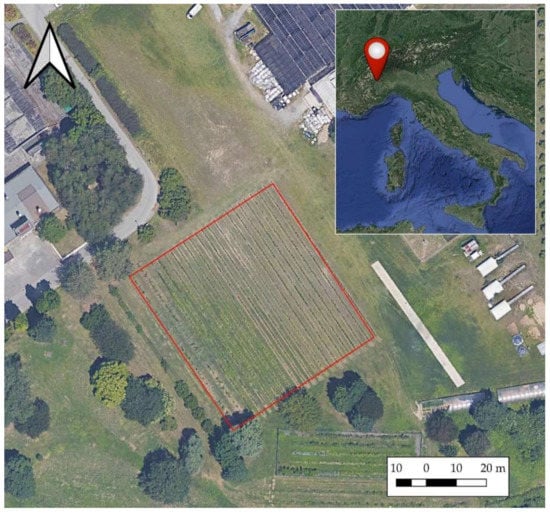
Figure 1.
Case study area: the vineyard in Grugliasco University (Piedmont Region, Italy), contoured by red line.
The vineyard extends for half a hectare and consists of 20 rows of different vine varieties, mainly Barbera, Nebbiolo, Moscato, Pinot Noir, and Sauvignon Blanc. The presence of many types is due to research purposes.
2.3. The Workflow
The workflow, shown in Figure 2, comprises three main phases:
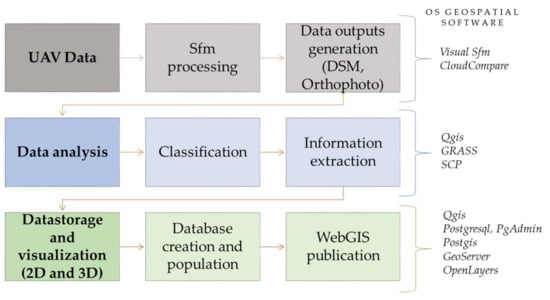
Figure 2.
The workflow of the methodology. SfM = Str5ucture from Motion; DSM = Digital Surface Model; SCP = Semi-Automatic Classification Plugin.
- drone mapping, data analysis, and information extraction;
- database construction;
- web-sharing.
Each step requires specific FOSS software, which differs in functionality and purpose.
2.3.1. Data Collection
As a first operation, it is necessary to acquire a complete representation of the area and therefore, a comprehensive survey of the entire area was carried out using a UAV.
Fifteen plastic markers, used as Ground Control Points (GCPs), were placed on the ground to allow a subsequent georeferencing of the digital model. The coordinates of the centre of each target were acquired using a Real-Time Kinematic (RTK) Global Navigation Satellite System (GNSS) technique [52]. For this application, which aims, as full detail, to identify the different plants within the rows, an accuracy of about 3–4 cm was enough for the elevation model and the orthophoto.
The UAV platform and the embedded sensors were selected according to the needs of the survey. Specifically, information regarding the infrared part of the electromagnetic spectrum was required to describe the vegetation efficiently [53]. Based on this, the multispectral camera SlantRange 4p+ was chosen. The kit of the camera consists of three elements (Table 1):

Table 1.
Data acquisition system specifications.
- a multispectral camera with four optical sensors:
- RGB (Center 470 nm (Blue) 520 nm (Green) 620 nm (Red), Width 110 nm);
- Red (Center 650 nm, Width 40 nm);
- Red Edge (Center 715 nm, Width 30 nm);
- Near IR (Center 850 nm, Width 70 nm);
- a Precision Navigation Module (LiDAR Rangefinder and Integrated Dual Antenna RTK GPS), which allows for obtaining better accuracy and quality of results in areas of uneven terrain [54];
- An Ambient Illumination Sensor (AIS) that allows for gaining sunlight-calibrated spectral images.
The SlantRange system needs the compatibility of the DJI SKYPORT as regards the UAV on which it is mounted. For this reason and, according to the SlantRange system weight of about 350 g, a DJI Matrice 210 V2 was used.
Then, based on the sensor and UAV’s characteristics, the flight was planned. The distance above the ground was about 70 m, to ensure a Ground Sample Distance (GSD) of about 1.5 cm on the object, in agreement with the survey requirements. A grid-schemed flight was carried out to obtain a total coverage of the area and an optimal overlap of the acquired images. The flight resulted in 465 images acquired for each SlantRange 4p+ sensor.
2.3.2. Data Processing
As a first pre-processing operation, the images acquired by the SlantRange system were calibrated with the software SlantView [54]. The sensor producer supplies this software, and it is part of the SlantRange system product. It processes the raw data recorded by the LiDAR module, the GPS/GNSS module and the Ambient Illumination Sensor, and extracts images radiometrically calibrated [55]. Moreover, Slantrange software allows separate of each band of the captured pictures in a single TIFF file.
After extracting the sets of calibrated images grouped by the band, the six datasets (one for each band of the electromagnetic spectrum: Blue, Green, Red W, Red N, Red Edge and NIR) were processed separately using the photogrammetric well-established Structure from Motion (SfM) approach [56]. SfM is now implemented in several commercial and FOSS software packages and, regardless of the software nature, it leads to the image alignment and generation of dense point clouds.
In this study, the photogrammetric process was carried out using Visual SfM [14,57] (FOSS). Several GCPs were collimated in the photos to georeference the photogrammetric block.
3D dense point clouds were produced with a high level of detail (about 28 million points for each set of images) (Figure 3 and Figure 4).
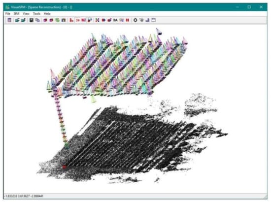
Figure 3.
Sparse cloud and cameras of the set relative to the RED W band.
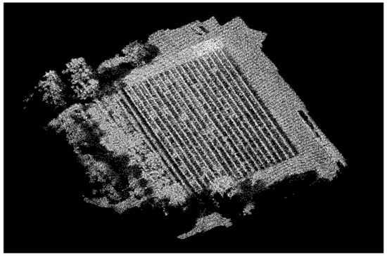
Figure 4.
Dense cloud relative to the RED W band in grey-level visualisation.
After generating six dense clouds, one for each set of images, they were imported in CloudCompare, an Open-source tool for the point cloud and mesh processing first developed by Daniel Girardeau-Montaut [58,59]. Finally, using the “rasterize” tool in Cloud Compare, which allows for transforming a point cloud into a 2.5D grid by setting the pixel size and the projection directions, the orthomosaics and the Digital Surface Model (DSM) were generated with a pixel size of 3 cm.
2.3.3. Mapping and Classification
The orthomosaics generated with the SfM technique were used to (i) map the vineyard rows and the single trees, and (ii) extract punctual information regarding the phenological conditions of the inter-row herbaceous vegetation.
First, a pixel-based supervised classification was performed that identified six classes (Table 2) using a Minimum Distance algorithm [60]. The classification was carried out in QGIS environment (version 3.14.0), using Gdal and Grass algorithms, and the QGIS semiautomatic classification plugin (SCP) developed by Luca Congedo [23].
Table 2.
Qualitative description of the classes according to first level classification (Classification I) and second-level classification (Classification II).
The structure of the classification was organised at two levels. The first level defined four classes (Shadows, Rows, Dense Herbaceous Vegetation, and Sparse Herbaceous Vegetation). The second level consisted of the reclassification of Shadows class to distinguish between Shaded Dense Herbaceous Vegetation and Shaded Sparse Herbaceous Vegetation. The Rows class helped in the definition of health condition of the vines. Shadows classes served the single-tree segmentation process and were used as geometry input, while the herbaceous vegetation classes described where under-row weeds needed to be mowed at the time of the survey.
Five derivative features were extracted from the Slantrange spectral bands to improve the classification’s final accuracy. These features are spectral indices that, along with the six Slantrange spectral bands and the DSM, constitute the final classification input dataset. Table 3 reports the list of the derivative features computed.
Table 3.
List of derivative features selected and used in the classification dataset.
Once the input dataset was created, a supervised classification was performed. Supervised classification algorithms require the definition of training samples. Thus, areas of class-homogeneous pixels and regions of interest (ROIs) were manually identified and made up the training dataset. Each ROI extends for 4180 pixels on average. Figure 5 shows the spectral signature of the classes and the scaled distance between each other.
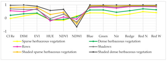
Figure 5.
Spectral signatures of the classes. The values were scaled on a −1—1 range to facilitate the reading of the graph.
The first level classification (Classification I) was performed using the Minimum Distance algorithm, with a threshold (standard deviation from the mean) of 2-sigma for classes Rows, Shaded Sparse Herbaceous Vegetation, Shaded Dense Herbaceous Vegetation, and Sparse Herbaceous Vegetation and 3-sigma for Shadows and Dense Herbaceous Vegetation. The result was then postprocessed applying a 15-pixel sieving filter and 4-pixel dilation on the Rows class. The areas classified as Shadows were masked and used for the second classification (Classification II). It was realised with the same algorithm and settings of Classification I. The main accuracy measures based on the error matrix (Producer’s accuracy, User’s accuracy, Overall accuracy, and F1-score) were computed for both classifications using 100 randomly placed points per class. The resulting classifications were merged.
The database built in this work also needs to store information at the single-tree level. The cultivation structure consisted of several grape trees in which vines grow together on three metal wires parallel to the ground. This structure made it impossible to detect each tree from the nadiral view of the rows. Thus, the single trees were segmented using the information derived from the shadows. The segmentation was performed on vector data. First, an intersection between the directional buffer of each row’s major axis and the shadows was computed and the centroids of the intersections were extracted.
Then, the centroids were snapped on the major axis of the rows. Voronoi polygons were computed on the centroid and clipped according to the row borders. Finally, the results were transformed from multipolygons to single polygons and visually checked. Figure 6 summarises the entire segmentation process.
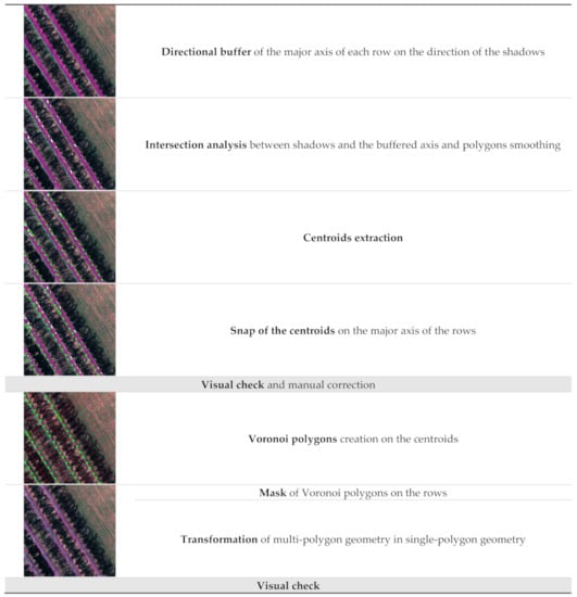
Figure 6.
Workflow for the detection of the single tree.
The modal values of the spectral indices EVI, NDVI, NDVI Red Edge, and Chlorophyll Index were then calculated and plotted for each object (tree) to scale the tree health [65].
3. Results and Discussion
The following sections present the outputs and outcomes of the described FOSS methodology: UAV survey processing products, classified data of rows and single-tree identification, and 2D and 3D web visualisation of data and attributes according to a structure geodatabase.
3.1. Orthophoto and DSM
Thanks to the operations described in Section 2.3, it was possible to extract orthophoto and DSM with the pixel size of 3 cm for each of the six bands separately. Figure 7 shows the DSM and the RGB orthomosaic obtained by the multichannel visualisation of Red, Green, and Blue bands.
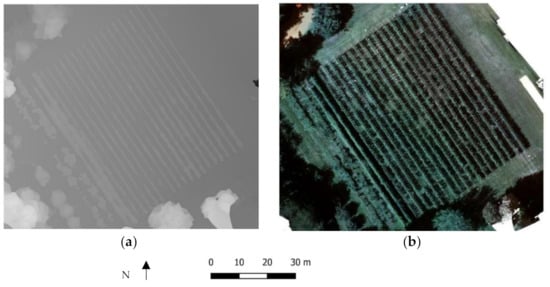
Figure 7.
(a) Digital Elevation Model (DEM), and (b) RGB orthophoto obtained by combining Red W, Green and Blue orthophotos.
It is worth notice that the SfM process required some practical measures to process multispectral data. The five multispectral bands were processed separately since Virtual SfM cannot deal with the 4p+ dataset.
3.2. Classification of the Rows and Single Tree Detection
The first classification was performed using the Minimum Distance algorithm on four classes with about 16,000 pixels as training. Its result shows some “salt and pepper” effect; indeed, some single pixels were not classified and some were misclassified (see Figure 8).
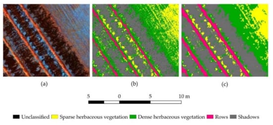
Figure 8.
Detail of the results of classification I. The (a) is the orthophoto in false colour (redEdge, Green, Red); (b) shows the classification I without postprocessing; (c) shows postprocessed classification I.
Nevertheless, these inaccuracies were corrected in the postprocessing phase through the sieving and dilation processes.
The final accuracy assessment on classification was measured on 400 points randomly placed, and it had an overall accuracy of 95% (Table 4). The Dense Herbaceous Vegetation represents the most critical classes and the Shadows as the F1-score indicates (respectively, 90% and 94%). This is mainly due to the difficulty of classification in the edge areas between the two classes. It is worth underlining that the shadows of the canopies’ upper parts are irregular and the illumination conditions are not uniform. The Producer’s accuracy is particularly low for the Dense Herbaceous Vegetation (only 0.87).
Table 4.
Error matrix of classification I. PA = Producer’s Accuracy; UA = User’s Accuracy; OA = Overall Accuracy.
Classification II was realised using the Minimum Distance algorithm on the pixels classified as Shadows from classification I. Only two classes are included in classification II: Shaded Sparse Herbaceous Vegetation and Shaded Dense Herbaceous Vegetation. Similarly to classification I, the results present some “salt and pepper” effect all over the scene of unclassified pixels, which was corrected in the postprocessing phase.
The accuracy assessment was measured on 200 randomly placed points, and it has an overall accuracy of 95% (Table 5). Eight validation points of Shaded Dense Herbaceous Vegetation were classified as Shaded Sparse Herbaceous Vegetation, and only two are in the opposite condition. The results of the accuracy measures are outstanding: both User’s and Producer’s accuracies were never below 92%. The presence of only two classes undoubtedly influences these positive results.
Table 5.
Error matrix of classification II. PA = Producer’s Accuracy; UA = User’s Accuracy; OA = Overall Accuracy.
The segmentation of single trees resulted in 1269 plants distributed on 20 rows. It is worth mentioning that the method does not provide the precise size of the canopies, but it assumes that the canopy of a grapevine is symmetrically developed on the metal wires and it extends until mid-distance to the next plant. This assumption is the base for using Voronoi polygon construction. Figure 9 shows the results of the classification and the segmentation.
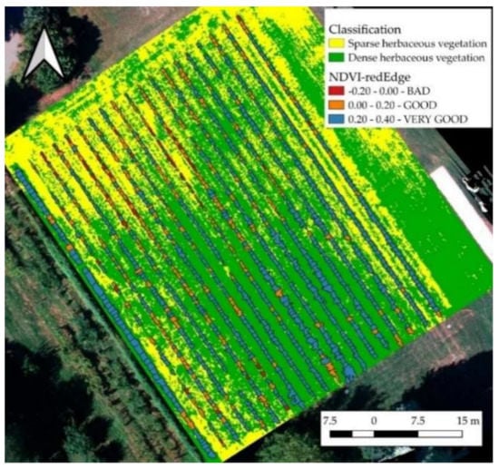
Figure 9.
The result of the classification and the segmentation of the single trees. The image shows the example of NDVI values calculated on the Red Edge band for each plant. NDVI-Red Edge was classified in BAD (<0.00), GOOD (0.00–0.20) and VERY GOOD (>0.20).
Finally, the EVI, NDVI, NDVI Red Edge, and Chlorophyll Index were calculated on the entire scene. The pixels’ mode value corresponding to single-tree geometries was calculated and scaled to identify the unhealthy plants.
3.3. Data Storage, Visualisation, and Querying
Following data generation, analysis and classification, the ending phases of the presented workflow aim to organise, store, visualise and query the postprocessed data. This final step, carried out by adopting open-source software, aims to develop a spatial database storing knowledge of vineyard and publishing information in a web- and user-friendly platform. This last process consists in the steps reported in Figure 10.
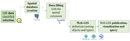
Figure 10.
Data visualisation and querying process.
For the generation and publication of the spatial dataset of the vineyard, different FOSS solutions were adopted. QGIS (version 3.14.0) was used for the database creation and for visualising 2D and 3D data, as Figure 6 shows (Section 2.3), while for the data publication, PostgreSQL with its interface PgAdmin, was selected. The spatial extension PostGIS was added for the geometry population. GeoServer, OpenLayer and Google Earth were used for the online publication of the database with three-dimensional visualisation and query elements. Figure 11 graphically describes the data storage, visualisation, and querying process.
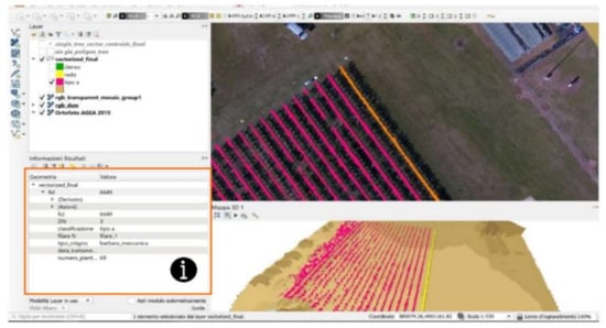
Figure 11.
QGIS project with 2D and 3D visualisation and querying of Grugliasco vineyard data.
3.3.1. 3D Visualisation of Data in QGIS and Spatial Database Creation
The first part of the methodological workflow regarded the QGIS project creation (Figure 11). This operation aimed to defined entities useful for the database creation to store information of the site area. Thanks to the 2D and 3D maps of Qgis, it was possible to plan a possible user-friendly web interface (explained in the next section). The following entities were selected to populate the table of attributes of the GIS project:
- DSM, raster data from drone acquisition;
- orthomosaic, raster data resulting from the SfM elaboration (Section 3.1) visualised in real colour (RGB);
- vineyard row, polygons obtained from the vectorisation of the class Rows;
- single trees and plants, centroid-points of the single tree;
- state of health, a classified vector composed polygons of single trees. It contains information regarding vegetation health indices.
In addition to the attributes derived from the data collected in the field, the classified vectors contain new attributes useful for the vineyard’s agricultural management, such as the identification number (ID), the grape variety, the number of rows, the history of phytosanitary treatments, and the number of vines. Further information can be added anytime. For example, as reported in the studies analysed in Section 1, it is possible to add additional data from national and international standards or based on the necessity of the performed analysis (such as soil description, climate conditions, characteristics of treetops, and variety of grape). Thanks to the new 3D Map implemented in QGIS, it was possible to visualise vector data on the surface model in 3D.
Then, the structure of the database was designed to support queries and data retrieval. A table of entities was created in PostgreSQL (Figure 12), and the column geometry was added thanks to the PostGIS extension. Then the geometries were populated connecting the database in QGIS by the DB manager tool, by setting the correct reference system (for this area WGS84-32N) and adding user and password of the localhost (PostgreSQL server works on port 5432).
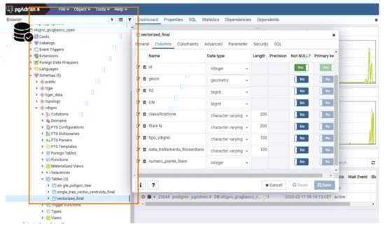
Figure 12.
Database tables creation in PostgreSQL (in the PgAdmin interface).
3.3.2. The WebGIS Platform
As mentioned before, the final output of this FOSS methodology consists of the WebGIS publication that allows any actors involved in the production of the grapes to interact with the 2D/3D database. To obtain a web address of the 2D model of the project, we selected GeoServer. It is an Open Source server for sharing geospatial data that provides maps and data such as web browsers and desktop GIS. Hence, it is possible to store spatial data in many formats, and users are not required to have GIS data structure knowledge. Moreover, GeoServer provides different types of data as well as vectors; Shapefiles; External WFS; PostGIS, ArcSDE, DB2, Oracle Spatial, MySql, SQL Server; Raster; GeoTiff, JPG and PNG; pyramids, GDAL formats, Image Mosaic, Oracle GeoRaster. It supports the EPSG projection as the WGS84-32N one.
Here the main steps are listed:
- Connection of the PostGIS Database in GeoServer with the localhost http://localhost:8080/geoserver/web, accessed on 5 April 2021;
- Workspace creation: Grugliasco vineyard (URI: http://localhost:8080/geoserver/Grugliascovineyard, accessed on 18 December 2020), Figure 13;
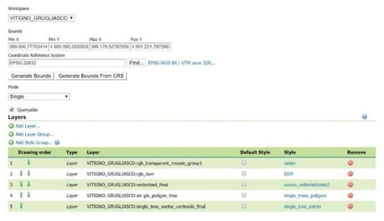 Figure 13. Workspace creation for the Grugliasco vineyard WebGIS.
 - Inserting layers from PostGIS (vectors and raster) with their style of visualisation. slt as defined in the QGIS project;
- Publication of the Grugliasco vineyard WebGIS in GeoServer;
- Visualisation of the 2D Map with OpenLayers (it is a JavaScript library for viewing interactive maps in web browsers) (Figure 14);
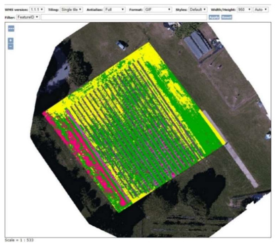 Figure 14. OpenLayers visualisation.
 - Downloading.kml, JSON or WFS file and 3D viewing in GIS environment or in Google Earth for a fast and for not-GIS specialised users’ immediate visualisation.
Finally, thanks to previous steps, it was possible to query the spatial data and the vineyard’s geometries, such as rows, trees, and plants, to gain all the information inserted in the QGIS project for the crop management.
The present research also tested another FOSS WebGIS solution using the QGIS plugin “QGIS2web” viewer and visualising the data of the WebMap with Leaflet (an open-source JavaScript library for mobile-friendly interactive maps [66]).
Despite the fact that this solution is faster and already integrated in the QGIS software, it does not provide the possibility to modify and implement the vineyard data into a spatial relational database structure. Indeed, it is not editable directly on the web using a FOSS GIS server.
4. Conclusions and Future Perspective
This paper presents a complete workflow based on FOSS procedure and software compared to the previous knowledge and the already published studies. The structure of the proposed workflow is the base for any applications based on SfM and automatic information extraction techniques. Indeed, it has a wide application range and can also be adapted to non-agricultural purposes, such as inventory management of cargo and urban green monitoring.
The paper aims to present and validate a FOSS workflow for smart farms and, at the same time, to point to possible future developments in this application field. This open-source research workflow starts with the acquisition phase of data with a multispectral sensor and traces the traditional photogrammetric process via SfM, classification of spatial data, and GIS visualization and querying processes adopting OS tools, combined under the precision agriculture hat. Moreover, the present study proposes a webGIS and user-friendly solution for smart farming, capable of garnering, updating, and querying information about crops and vineyard processes in a unique spatial database system. The reliability of the whole process is demonstrated with a real case study used for testing the single steps and validating them.
Although the three main steps of the workflow could be applied and validated separately, the methodology assessment could be improved. With this in mind, the present research tends to set the base for the following developments. Hence, future works should focus on evaluating the workflow in terms of effectiveness and replicability. The effectiveness concerns the workflow’s appropriateness to answer the PA’s needs and can be evaluated via subjective qualitative methods, such as questionnaires and interviews to final users, and objective methods, through reliable indicators. This evaluation needs to be carried out after a significant time of usage of the webGIS platform and its data implementation.
The presented solution is easily replicable by many use cases and by different stakeholders involved in various tasks concerning precision agriculture. As mentioned in [67], the integration of geomatics techniques and methods (such as remote sensing and aerial photogrammetry by different sensors) with a geographic information system could improve the resilience of modern agriculture, managing and monitoring every step (seeding, crop growth, and harvesting and production).
Additionally, the methods’ replicability can be assessed on similar case studies or compared with commercial solutions. It is worth mentioning that the three main steps of the proposed workflow remain unaltered regardless of the study case. Nevertheless, from the replicability point of view, adjustments could be necessary for what concerns the classification. The classification parameters depend on the defining characteristics of the vineyard and the possible input data type (i.e., RGB, multispectral).
Moreover, the spatial database can be implemented and organized to store precision farming information collected by OS hardware, making a step toward OS smart farming. Total OS smart farming is the expected direction for future research.
Another fundamental aspect to take into consideration regards the possibility of targeting a wider audience, now designated to not-academic or not-GIS expert users, enriching the web-GIS DB-based platform with analysis tools and giving different level of access depending on the degree of expertise.
Future steps of our research could consider creating a new web service able to support field operation for treatments of grapes and crops, providing online digital content (also accessible from mobile devices). Even if some valuable examples of digital tools are already developed in the vineyard management field, none of these present map services or spatial datasets.
Author Contributions
Conceptualisation, Elena Belcore, Stefano Angeli, Elisabetta Colucci, Maria Angela Musci, and Irene Aicardi; methodology, Elena Belcore, Stefano Angeli, and Elisabetta Colucci; software, Elena Belcore, Stefano Angeli, and Elisabetta Colucci; validation, Elena Belcore, Stefano Angeli, and Elisabetta Colucci; formal analysis, Elena Belcore, Stefano Angeli, and Elisabetta Colucci; investigation, Elena Belcore, Stefano Angeli, Elisabetta Colucci, and Maria Angela Musci; resources, Elena Belcore, Stefano Angeli, Elisabetta Colucci, and Maria Angela Musci; data curation, Elena Belcore, Stefano Angeli, and Elisabetta Colucci; writing—original draft preparation Elena Belcore, Stefano Angeli, Elisabetta Colucci, and Maria Angela Musci; writing—review and editing, Elena Belcore, Stefano Angeli, Elisabetta Colucci, Maria Angela Musci, and Irene Aicardi; supervision, Irene Aicardi; project administration, Irene Aicardi. All authors have read and agreed to the published version of the manuscript.
Funding
This research received no external funding.
Institutional Review Board Statement
Not applicable.
Informed Consent Statement
Not applicable.
Data Availability Statement
The data presented in this study are available on request from the corresponding author.
Acknowledgments
This project was carried out within the activities of the PoliTO Interdepartmental Centre for Service Robotics (PIC4SeR) [68]. The authors would like to acknowledge “Dipartimento di Scienze Agrarie, Forestali e Alimentari” (DISAFA) of Università di Torino for giving the chance to use their vineyards as study cases.
Conflicts of Interest
The authors declare no conflict of interest.
References
- Coetzee, S.; Ivánová, I.; Mitasova, H.; Brovelli, M.A. Open Geospatial Software and Data: A Review of the Current State and A Perspective into the Future. ISPRS Int. J. Geo-Inf. 2020, 9, 90. [Google Scholar] [CrossRef]
- Mobasheri, A.; Mitasova, H.; Neteler, M.; Singleton, A.; Ledoux, H.; Brovelli, M.A. Highlighting recent trends in open source geospatial science and software. Trans. GIS 2020, 24, 1141–1146. [Google Scholar] [CrossRef]
- Brovelli, M.A.; Mitasova, H.; Neteler, M.; Raghavan, V. Free and open source desktop and Web GIS solutions. Appl. Geomat. 2012, 4, 65–66. [Google Scholar] [CrossRef]
- Steiniger, S.; Hunter, A.J.S. The 2012 free and open source GIS software map—A guide to facilitate research, development, and adoption. Comput. Environ. Urban Syst. 2013, 39, 136–150. [Google Scholar] [CrossRef]
- QGIS Development Team QGIS. Un Sistema Di Informazione Geografica Libero e Open Source. Available online: https://qgis.org/it/site/ (accessed on 15 January 2021).
- Böhner, J.; Conrad, O. SAGA-System for Automated Geoscientific Analyses. Available online: http://www.saga-gis.org/en/index.html (accessed on 15 January 2021).
- GRASS Development Team GRASS GIS-Bringing Advanced Geospatial Technologies to the World. Available online: https://grass.osgeo.org/ (accessed on 15 January 2021).
- GDAL. GDAL Documentation. Available online: https://gdal.org/ (accessed on 15 January 2021).
- PostgreSQL Global Development Group PostgreSQL. Available online: https://www.postgresql.org/ (accessed on 15 January 2021).
- GeoServer. Available online: http://geoserver.org/ (accessed on 15 January 2021).
- Open Source Geospatial Foundation. MapServer 7.6.2 Documentation. Available online: https://mapserver.org/ (accessed on 15 January 2021).
- GeoNode. Available online: https://geonode.org/ (accessed on 15 January 2021).
- MicMac. Available online: https://micmac.ensg.eu/index.php/Accueil (accessed on 15 January 2021).
- Wu, C. VisualSFM: A Visual Structure from Motion System. Available online: http://ccwu.me/vsfm/ (accessed on 15 January 2021).
- OpenDroneMap Contributors. Drone Mapping Software. Available online: https://www.opendronemap.org/ (accessed on 15 January 2021).
- Grasso, S.; Claps, P.; Ganora, D.; Libertino, A. A Web-based Open-source Geoinformation Tool for Regional Water Resources Assessment. Water Resour. Manag. 2021, 35, 675–687. [Google Scholar] [CrossRef]
- Wei, M.; Liu, T.; Sun, B. Optimal Routing Design of Feeder Transit With Stop Selection Using Aggregated Cell Phone Data and Open Source GIS Tool. IEEE Trans. Intell. Transp. Syst. 2021, 1–12. [Google Scholar] [CrossRef]
- Liu, X.; Long, Y. Automated Identification and Characterization of Parcels with OpenStreetMap and Points of Interest. Environ. Plan. B Plan. Des. 2016, 43, 341–360. [Google Scholar] [CrossRef]
- Mobasheri, A. (Ed.) An Introduction to Open Source Geospatial Science for Urban Studies. In Open Source Geospatial Science for Urban Studies: The Value of Open Geospatial Data; Springer: Cham, Switzerland, 2021; pp. 1–8. [Google Scholar]
- Bhunia, G.S.; Shit, P.K.; Sengupta, D. Free-Open Access Geospatial Data and Tools for Forest Resources Management. In Spatial Modeling in Forest Resources Management: Rural Livelihood and Sustainable Development; Shit, P.K., Pourghasemi, H.R., Das, P., Bhunia, G.S., Eds.; Springer: Cham, Switzerland, 2021; pp. 651–675. [Google Scholar]
- Takasu, T.; Yasuda, A. Development of the Low-Cost RTK-GPS Receiver with an Open Source Program Package RTKLIB. In Proceedings of the International Symposium on GPS/GNSS, Karlsruhe, Germany, 22–23 September 2009; p. 6. [Google Scholar]
- Orfeo ToolBox–Orfeo ToolBox Is Not a Black Box. Available online: https://www.orfeo-toolbox.org/ (accessed on 10 January 2021).
- Congedo, L. Semi-Automatic Classification Plugin Documentation. Available online: https://semiautomaticclassificationmanual-v5.readthedocs.io/en/latest/ (accessed on 3 February 2021).
- Saiz-Rubio, V.; Rovira-Más, F. From Smart Farming towards Agriculture 5.0: A Review on Crop Data Management. Agronomy 2020, 10, 207. [Google Scholar] [CrossRef]
- Ono, T.; Iida, K.; Yamazaki, S. Achieving Sustainable Development Goals (SDGs) through ICT Services. Fujitsu Sci. Tech. J. 2017, 53, 17–22. [Google Scholar]
- United Nations. The Sustainable Development Goals Report 2019; United Nations: New York, NY, USA, 2019. [Google Scholar]
- Bramley, R.G.V. Progress in the Development of Precision Viticulture-Variation in Yield, Quality and Soil Proporties in Contrasting Australian Vineyards; Australian Wine Research Institute: Victoria, Australia, 2001. [Google Scholar]
- Zarco-Tejada, P.J.; Hubbard, N.; Loudjani, P. Precision Agriculture: An Opportunity for EU Farmers: Potential Support with the CAP 2014–2020; European Commission: Brussels, Belgium, 2014; p. 56. [Google Scholar]
- Cook, S.E.; Bramley, R.G.V. Precision agriculture—Opportunities, benefits and pitfalls of site-specific crop management in Australia. Aust. J. Exp. Agric. 1998, 38, 753–763. [Google Scholar] [CrossRef]
- Caffaro, F.; Cavallo, E. The Effects of Individual Variables, Farming System Characteristics and Perceived Barriers on Actual Use of Smart Farming Technologies: Evidence from the Piedmont Region, Northwestern Italy. Agriculture 2019, 9, 111. [Google Scholar] [CrossRef]
- Kritikos, M. Precision Agriculture in Europe: Legal, Social and Ethical Considerations; European Parliamentary Research Service: Brussels, Belgium, 2017. [Google Scholar]
- Mesas-Carrascosa, F.J.; Santano, D.V.; Meroño, J.E.; de la Orden, M.S.; García-Ferrer, A. Open source hardware to monitor environmental parameters in precision agriculture. Biosyst. Eng. 2015, 137, 73–83. [Google Scholar] [CrossRef]
- Adenle, A.A.; Sowe, S.K.; Parayil, G.; Aginam, O. Analysis of open source biotechnology in developing countries: An emerging framework for sustainable agriculture. Technol. Soc. 2012, 34, 256–269. [Google Scholar] [CrossRef]
- Gitelson, A.A.; Viña, A.; Arkebauer, T.J.; Rundquist, D.C.; Keydan, G.; Leavitt, B. Remote estimation of leaf area index and green leaf biomass in maize canopies. Geophys. Res. Lett. 2003, 30. [Google Scholar] [CrossRef]
- Krintz, C.; Liu, B. SmartFarm: Improving Agriculture Sustainability Using Modern Information Technology; University of California: Santa Barbara, CA, USA, 2016; p. 6. [Google Scholar]
- Matese, A.; Di Gennaro, S.F. Practical Applications of a Multisensor UAV Platform Based on Multispectral, Thermal and RGB High Resolution Images in Precision Viticulture. Agriculture 2018, 8, 116. [Google Scholar] [CrossRef]
- Filippis, T.D.; Rocchi, L.; Fiorillo, E.; Genesio, L. A WebGIS application for precision viticulture: From research to operative practices. Available online: https://www.isprs.org/proceedings/XXXVIII/4-W13/ID_69.pdf (accessed on 6 February 2021).
- Rokhmana, C.A. The Potential of UAV-Based Remote Sensing for Supporting Precision Agriculture in Indonesia. Procedia Environ. Sci. 2015, 24, 245–253. [Google Scholar] [CrossRef]
- Puri, V.; Nayyar, A.; Raja, L. Agriculture drones: A modern breakthrough in precision agriculture. J. Stat. Manag. Syst. 2017, 20, 507–518. [Google Scholar] [CrossRef]
- Podagrosi, A. A FOSS Web Mapping Solution for Disparate Precision Agriculture Data. In Proceedings of the FOSS4G, Boston, MA, USA, 14–19 August 2017; p. 14. [Google Scholar]
- Trilles, S.; Torres-Sospedra, J.; Belmonte, Ó.; Zarazaga-Soria, F.J.; González-Pérez, A.; Huerta, J. Development of an open sensorized platform in a smart agriculture context: A vineyard support system for monitoring mildew disease. Sustain. Comput. Inform. Syst. 2019, 100309. [Google Scholar] [CrossRef]
- Ye, J.; Chen, B.; Liu, Q.; Fang, Y. A precision agriculture management system based on Internet of Things and WebGIS. In Proceedings of the 21st IEEE International Conference on Geoinformatics, Kaifeng, China, 20–22 June 2013. [Google Scholar] [CrossRef]
- Brocchini, D.; Chiabrando, F.; Colucci, E.; Sammartano, G.; Spanò, A.; Losè, L.T.; Villa, A. The Geomatics Contribution for the Valorisation Project in the Rocca of San Silvestro Landscape Site. ISPRS Int. J. Geo Inf. 2017, 42, 495–502. [Google Scholar] [CrossRef]
- Colucci, E. Architettura e Natura Di Paesaggi Archeologici Analisi Spaziali Integrate in Ambiente WEB-GIS per La Conservazione e La Comunicazione Della Memoria Storica: Il Parco Archeominerario Di San Silvestro. Master’s Thesis, Politecnico di Torino, Turin, Italy, 2017. [Google Scholar]
- Brovelli, M.A.; Magni, D. An Archaeological Web Gis Application Based on Mapserver and Postgis. Available online: https://www.isprs.org/proceedings/XXXIV/5-W12/proceedings/19.pdf (accessed on 3 March 2021).
- Grecea, C.; Herban, S.; Vilceanu, C.-B. WebGIS Solution for Urban Planning Strategies. Procedia Eng. 2016, 161, 1625–1630. [Google Scholar] [CrossRef]
- Pierce, F.J.; Clay, D. (Eds.) GIS Applications in Agriculture; CRC Press: Boca Raton, FL, USA, 2007. [Google Scholar]
- Open Geospatial Consortium. Finding OGC WMS, WFS, WCS Services. Available online: https://www.ogc.org/blog/2034 (accessed on 15 January 2021).
- European Commission: INSPIRE. Available online: https://inspire.ec.europa.eu/ (accessed on 15 January 2021).
- Mazzetto, F.; Gallo, R.; Sacco, P. Reflections and Methodological Proposals to Treat the Concept of “Information Precision” in Smart Agriculture Practices. Sensors 2020, 20, 2847. [Google Scholar] [CrossRef]
- Brancadoro, L.; Carnevali, P. Proximal Sensing per la Viticoltura Sito-Specifica. Available online: http://www.ricercatuscania.it/data/files/finale/4_Linea_A2_Diprove.pdf (accessed on 6 April 2021).
- Cina, A.; Dabove, P.; Manzino, A.M.; Piras, M. Network Real Time Kinematic (NRTK) Positioning–Description, Architectures and Performances. In Satellite Positioning—Methods, Models and Applications; IntechOpen: London, UK, 2015. [Google Scholar] [CrossRef]
- Kumar, L.; Schmidt, K.; Dury, S.; Skidmore, A. Imaging Spectrometry and Vegetation Science. In Imaging Spectrometry: Basic Principles and Prospective Applications; Springer: Berlin/Heidelberg, Germany, 2002; pp. 111–155. [Google Scholar]
- SlantRange. Precision Agriculture Technology, Sensors and Analytics. Available online: https://slantrange.com/ (accessed on 15 January 2021).
- Wagner, W. Radiometric calibration of small-footprint full-waveform airborne laser scanner measurements: Basic physical concepts. ISPRS Int. J. Geo Inf. 2010, 65, 505–513. [Google Scholar] [CrossRef]
- Turner, D.; Lucieer, A.; Watson, C. An Automated Technique for Generating Georectified Mosaics from Ultra-High Resolution Unmanned Aerial Vehicle (UAV) Imagery, Based on Structure from Motion (SfM) Point Clouds. Remote Sens. 2012, 4, 1392–1410. [Google Scholar] [CrossRef]
- Wu, C.; Agarwal, S.; Curless, B.; Seitz, S.M. Multicore bundle adjustment. In Proceedings of the 24th IEEE Conference on Computer Vision and Pattern Recognition, Colorado Springs, CO, USA, 20–25 June 2011; pp. 3057–3064. [Google Scholar]
- PASTEL. Available online: https://web.archive.org/web/20071227030420/http://pastel.paristech.org/1745/ (accessed on 18 December 2020).
- CloudCompare—Open Source Project. Available online: http://www.cloudcompare.org/ (accessed on 18 December 2020).
- Richards, J.A.; Jia, X. Remote Sensing Digital Image Analysis: An Introduction, 4th ed.; Springer: Berlin/Heidelberg, Germany, 2006. [Google Scholar]
- Huete, A.; Justice, C.; Liu, H. Development of vegetation and soil indices for MODIS-EOS. Remote. Sens. Environ. 1994, 49, 224–234. [Google Scholar] [CrossRef]
- Henrich, V.; Krauss, G.; Götze, C.; Sandow, C. The IndexDatabase; University of Bonn: Bonn, Germany, 2011. [Google Scholar]
- Rouse, J.W. Monitoring the Vernal Advancement and Netrogradation of Natural Vegetation; Texas A&M University: College Station, TX, USA, 1973. [Google Scholar]
- McFeeters, S.K. The use of the Normalized Difference Water Index (NDWI) in the delineation of open water features. Int. J. Remote Sens. 1996, 17, 1425–1432. [Google Scholar] [CrossRef]
- Taskos, D.G.; Koundouras, S.; Stamatiadis, S.; Zioziou, E.; Nikolaou, N.; Karakioulakis, K.; Theodorou, N. Using active canopy sensors and chlorophyll meters to estimate grapevine nitrogen status and productivity. Precis. Agric. 2015, 16, 77–98. [Google Scholar] [CrossRef]
- Agafonkin, V. Leaflet—A JavaScript Library for Interactive Maps. Available online: https://leafletjs.com/ (accessed on 15 January 2021).
- Jung, J.; Maeda, M.; Chang, A.; Bhandari, M.; Ashapure, A.; Landivar-Bowles, J. The potential of remote sensing and artificial intelligence as tools to improve the resilience of agriculture production systems. Curr. Opin. Biotechnol. 2021, 70, 15–22. [Google Scholar] [CrossRef] [PubMed]
- PIC4SeR PoliTO Interdepartmental Centre for Service Robotics. Available online: https://pic4ser.polito.it/ (accessed on 6 April 2021).


Publisher’s Note: MDPI stays neutral with regard to jurisdictional claims in published maps and institutional affiliations. |
© 2021 by the authors. Licensee MDPI, Basel, Switzerland. This article is an open access article distributed under the terms and conditions of the Creative Commons Attribution (CC BY) license (https://creativecommons.org/licenses/by/4.0/).