
End Point Rate Tool for QGIS (EPR4Q): Validation Using DSAS and AMBUR

 ,
,  ,
,
Abstract
1. Introduction
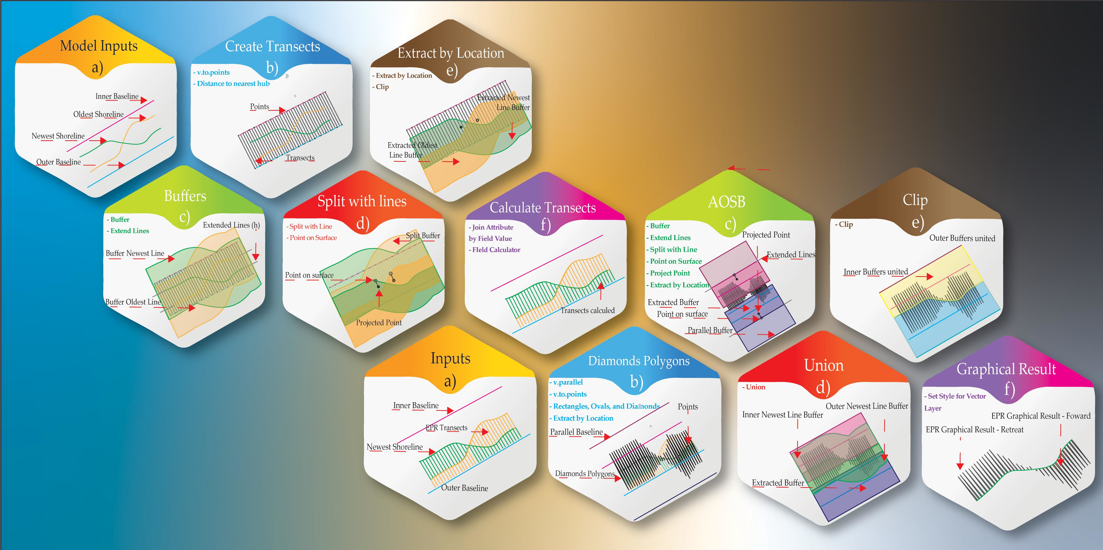
2. Study Areas
3. Materials and Methods
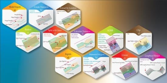
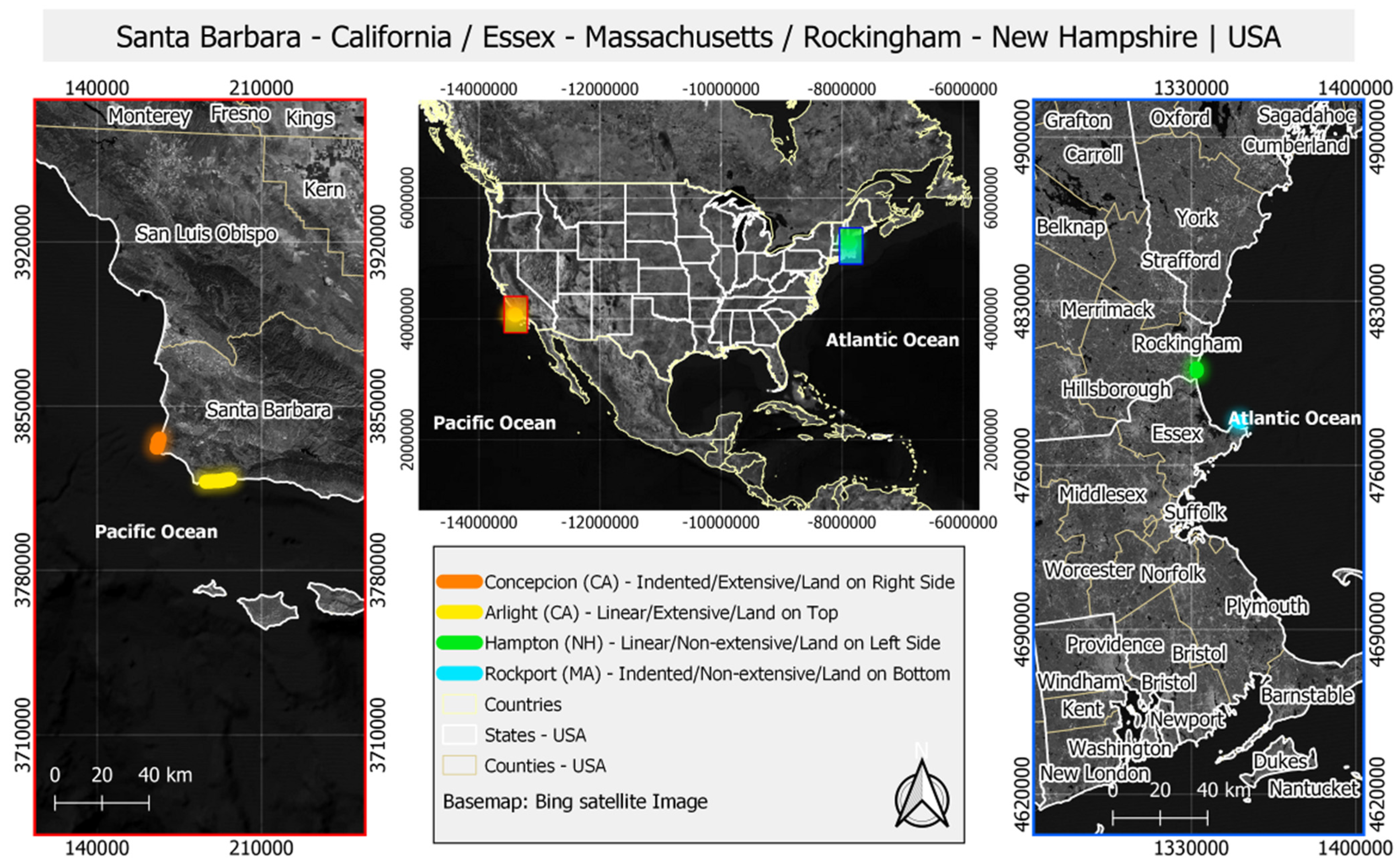
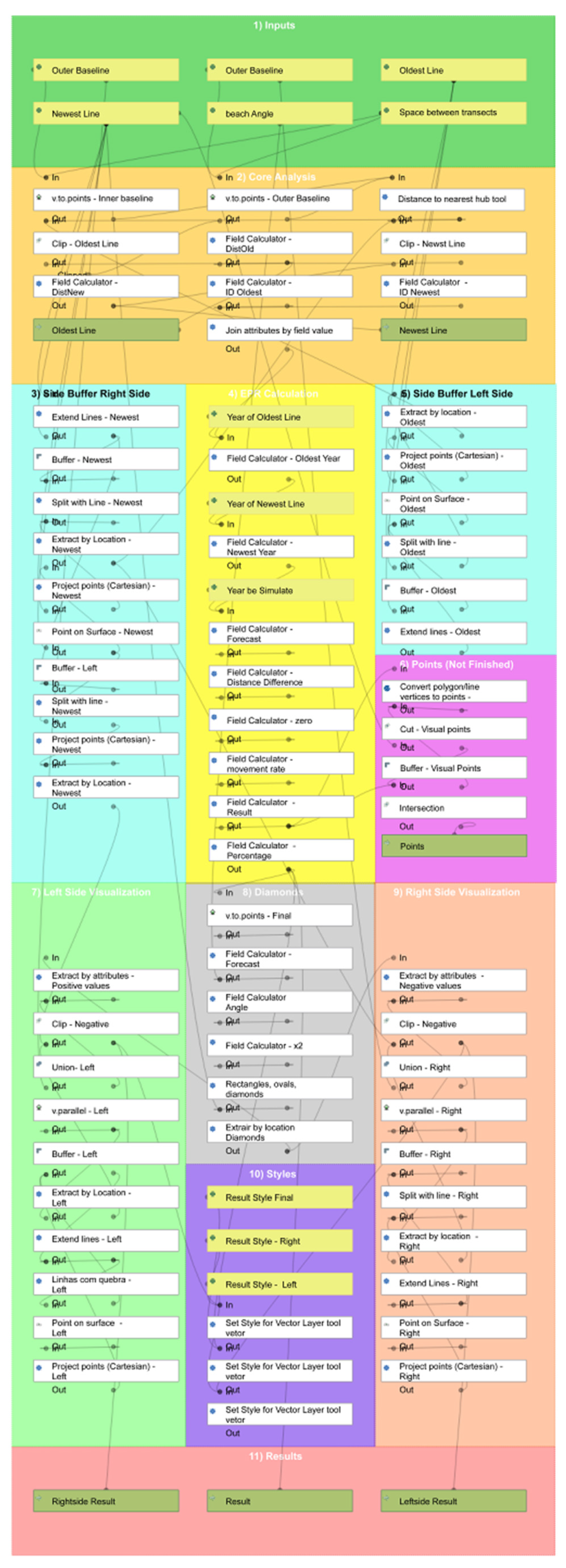
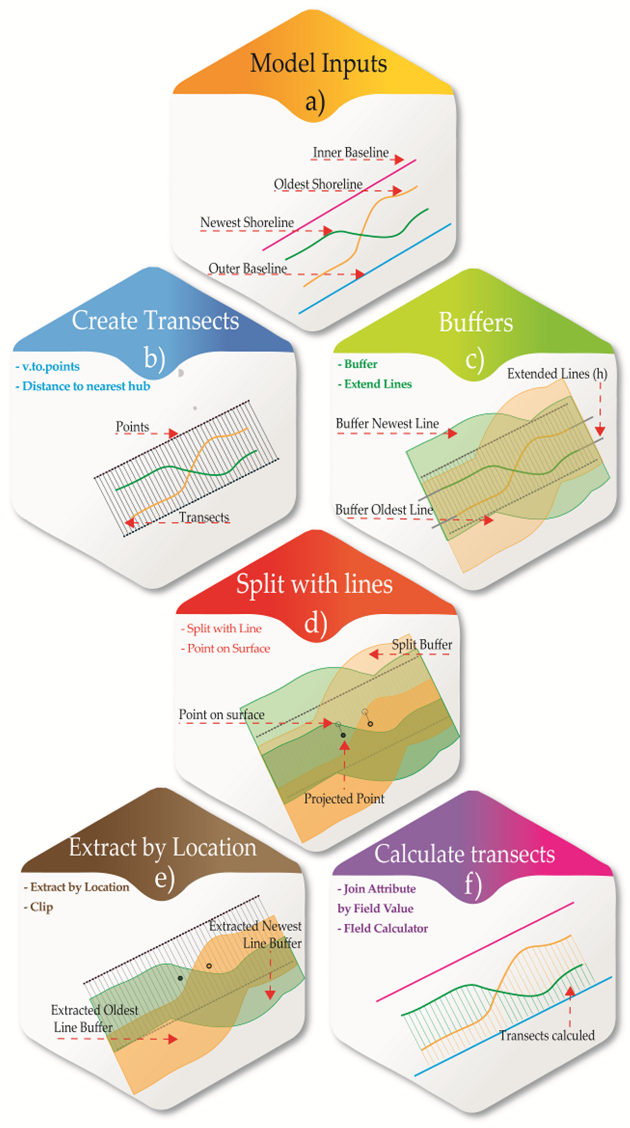
3.1. EPR4Q Tool Creation
3.1.1. EPR Method
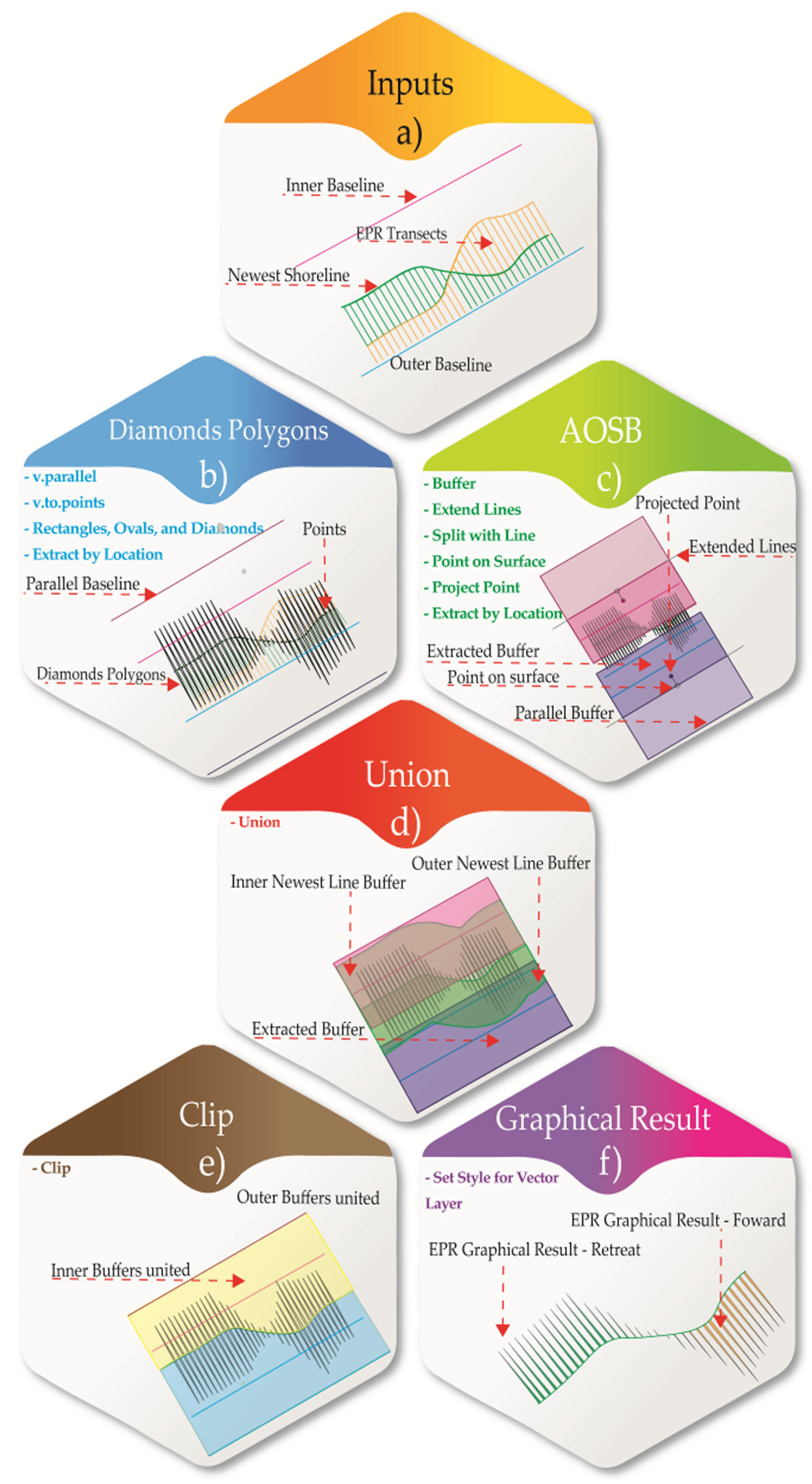
3.1.2. EPR Forecast and Visualization
3.2. Validation Process
3.2.1. Shorelines Data
3.2.2. Transects Selection and Statistical Analysis
4. Results
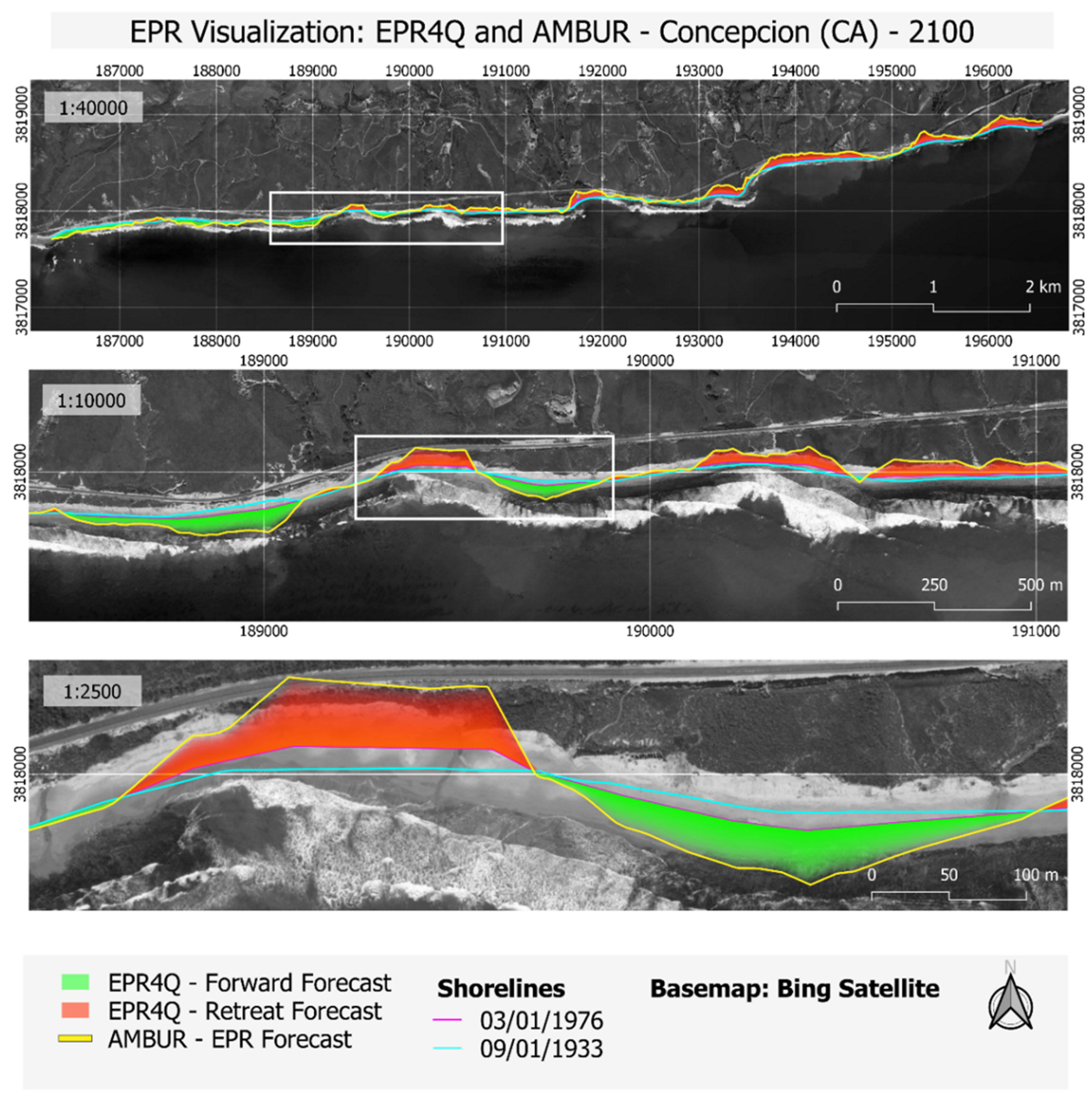
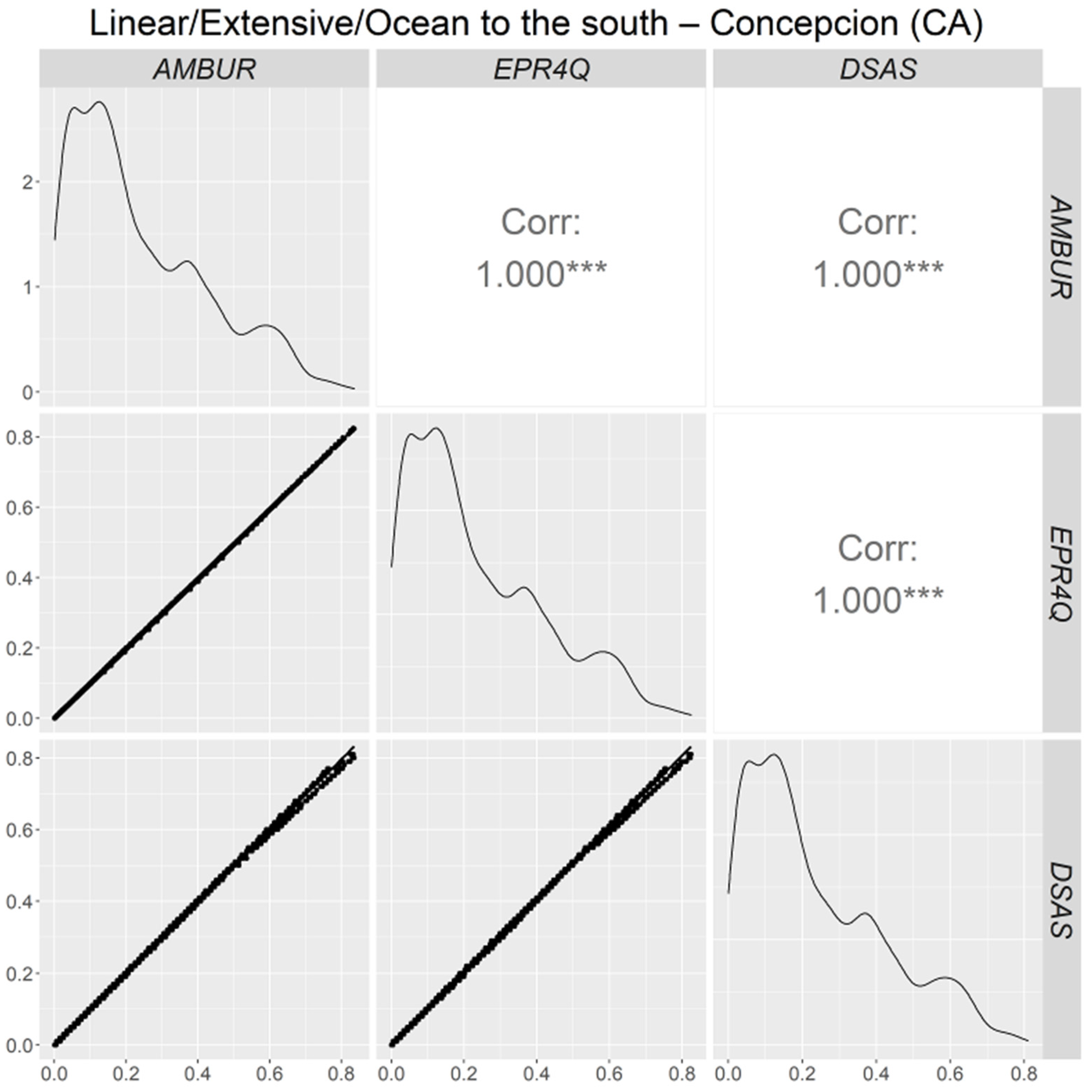
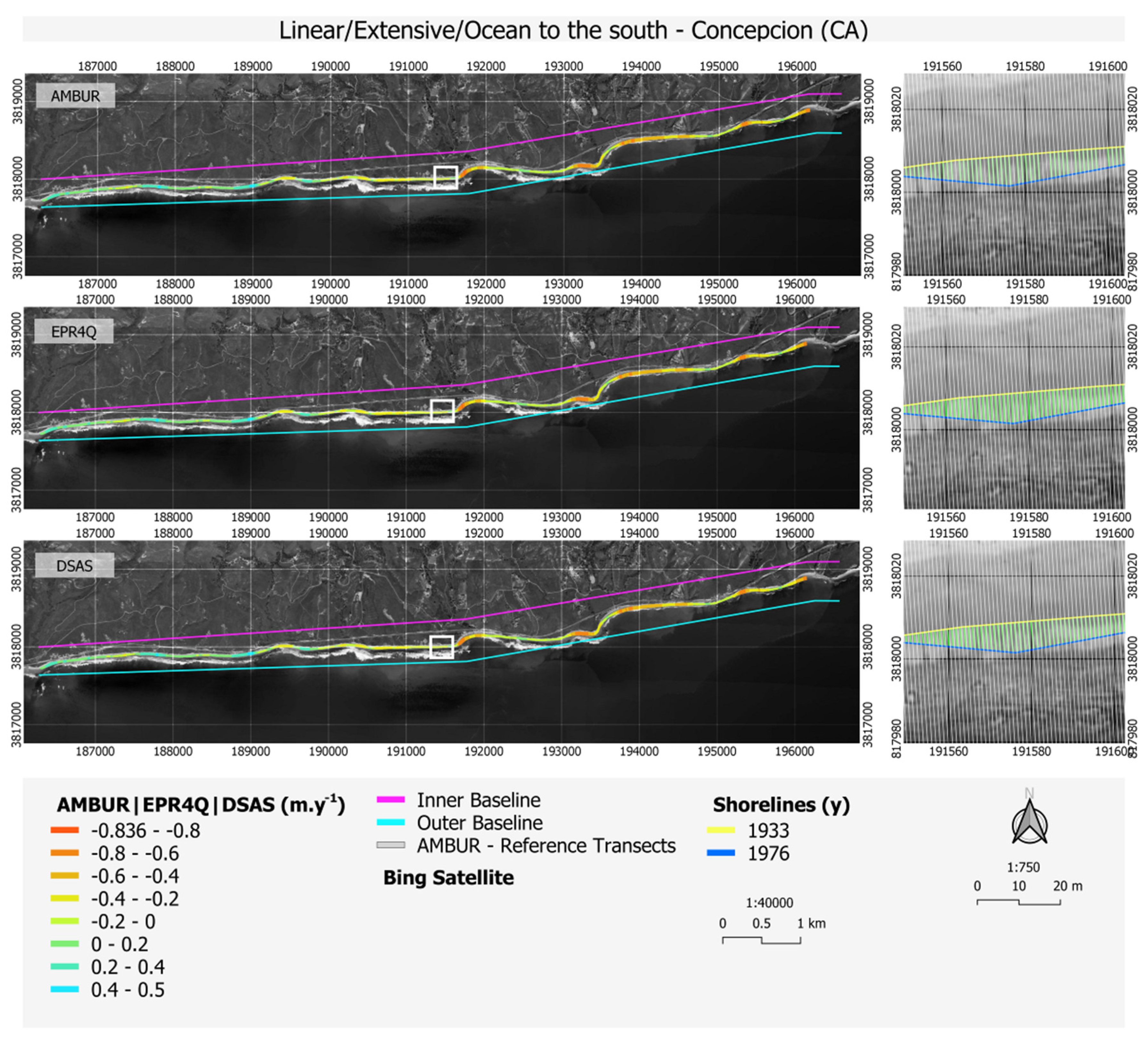
4.1. Linear/Extensive/Ocean to the South—Concepcion (CA)
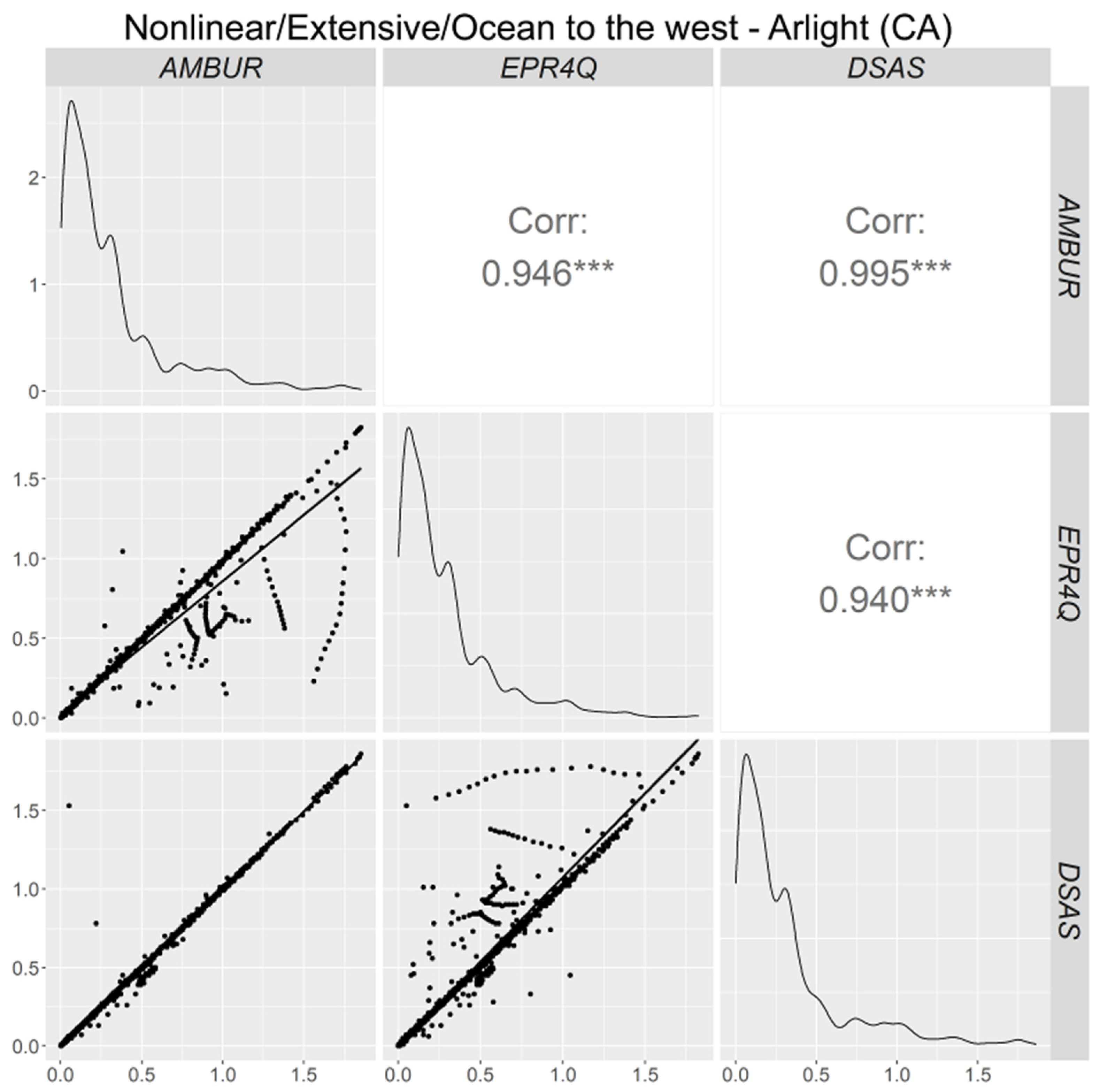
4.2. Nonlinear/Extensive/Ocean to the West—Arlight (CA)
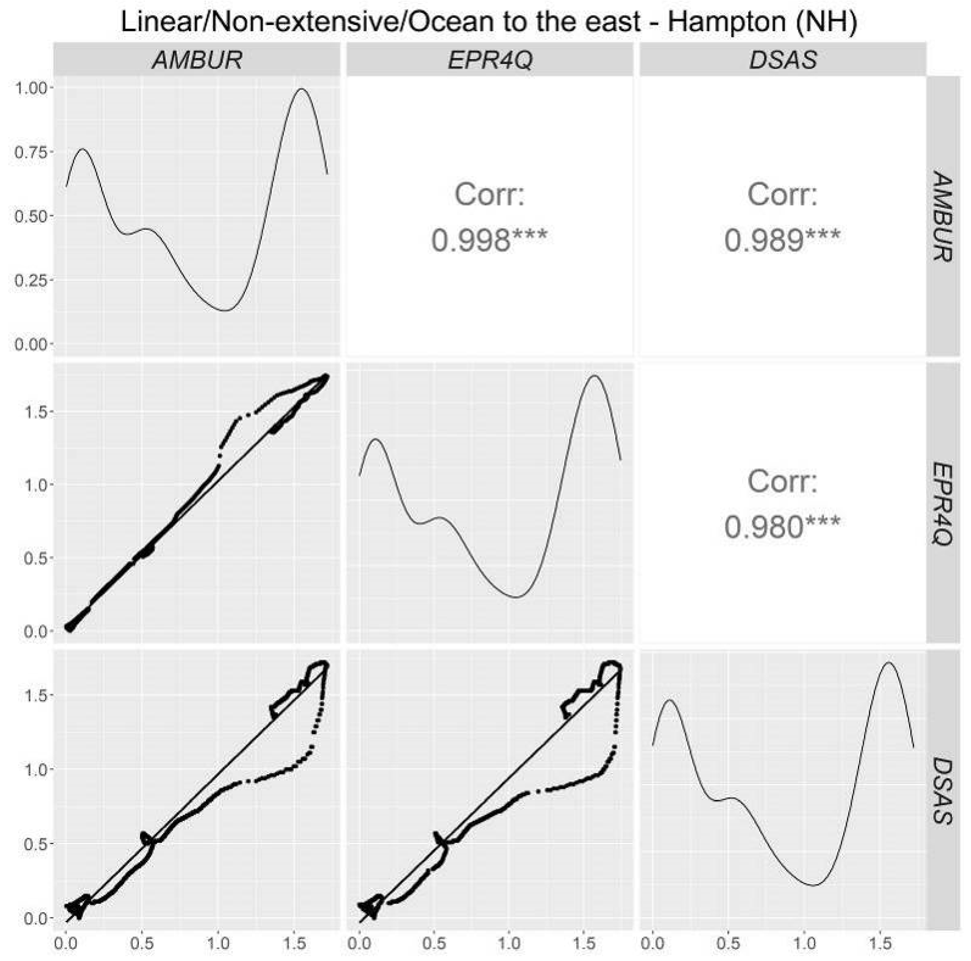
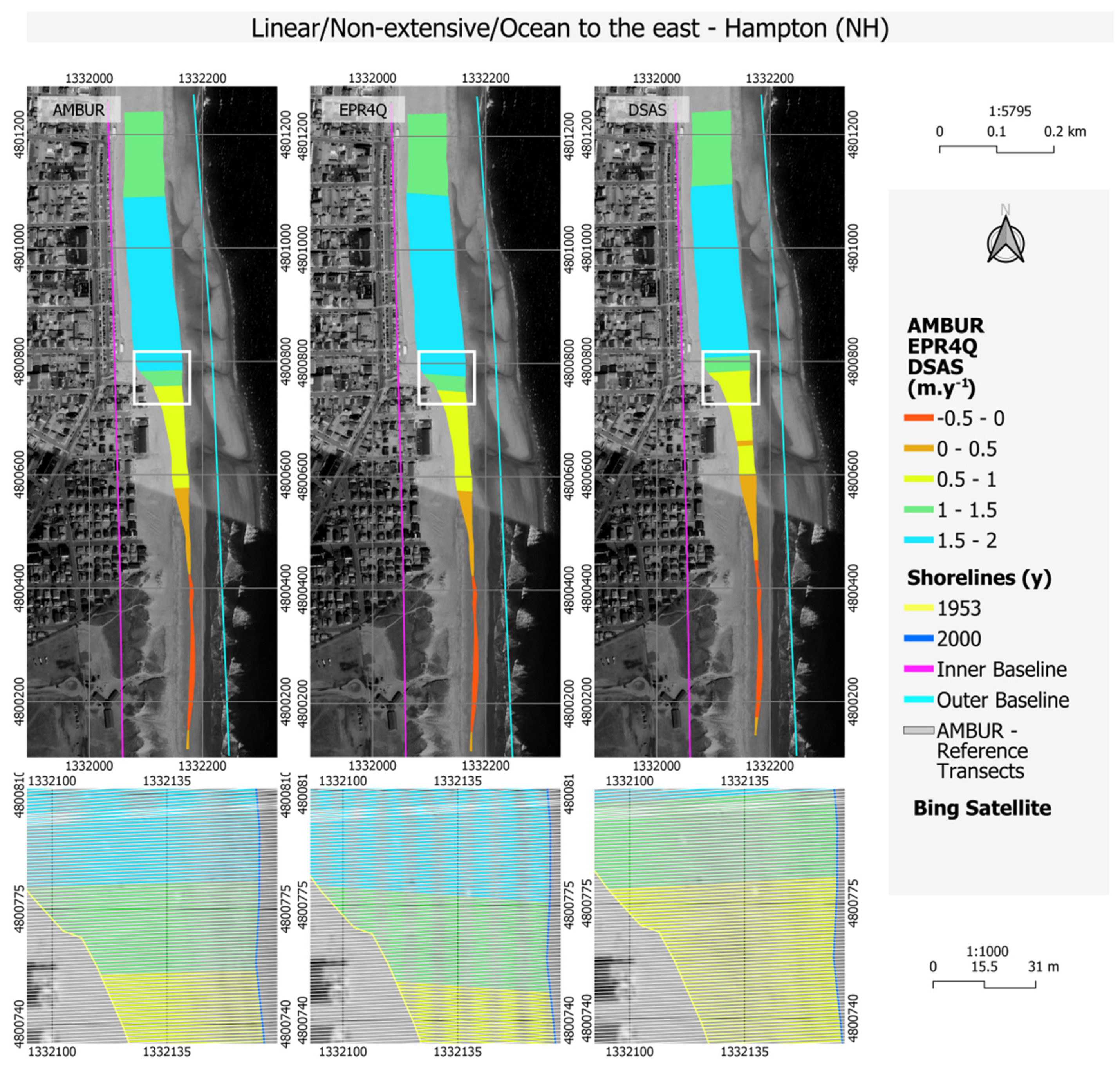
4.3. Linear/Non-Extensive/Ocean to the East—Hampton (NH)
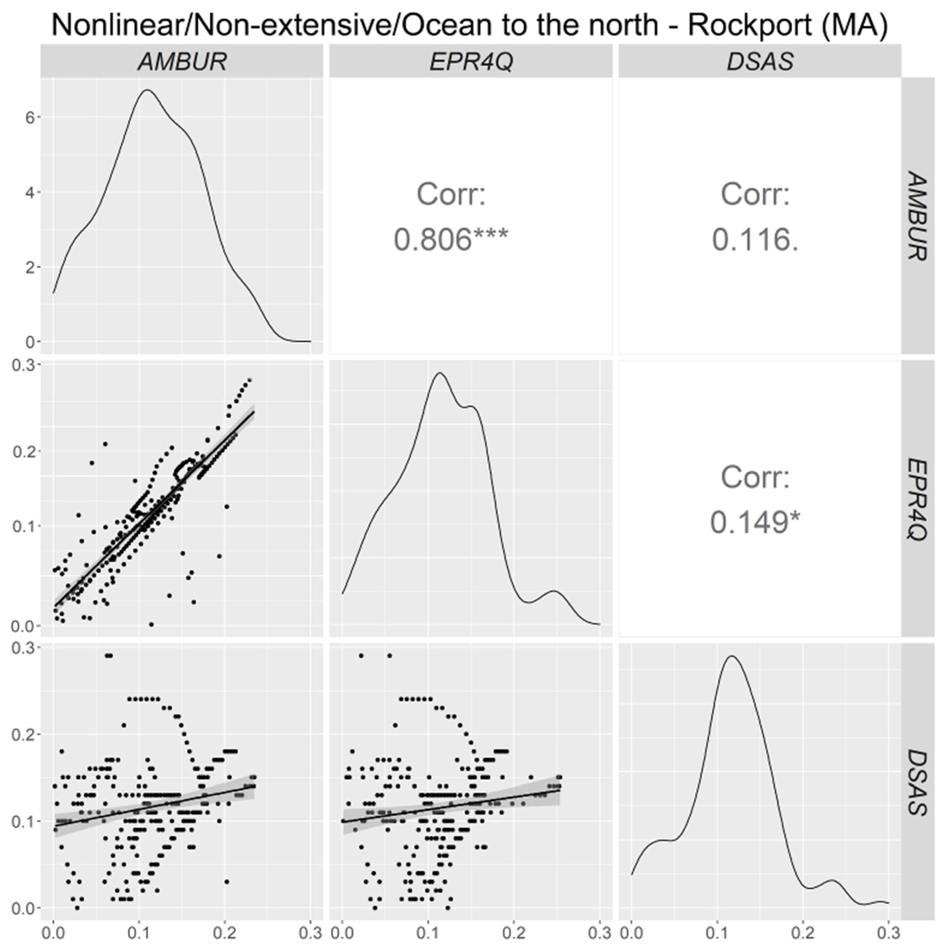
4.4. Nonlinear/Non-Extensive/Ocean to the North—Rockport (MA)
5. Discussion
6. Conclusions
Author Contributions
Funding
Data Availability Statement
Acknowledgments
Conflicts of Interest
References
- Luijendijk, A.; Hagenaars, G.; Ranasinghe, R.; Baart, F.; Donchyts, G.; Aarninkhof, S. The State of the World’s Beaches. Sci. Rep. 2018, 8, 6641. [Google Scholar] [CrossRef]
- Dritsas, S.E. The effect of sea level rise on coastal populations: The case of the Gironde (Estuaries of Gironde). Econ. Anal. Policy 2020, 66, 41–50. [Google Scholar] [CrossRef]
- Boak, E.H.; Turner, I.L. Shoreline definition and detection: A review. J. Coast. Res. 2005, 21, 688–703. [Google Scholar] [CrossRef]
- Crowell, M.; Leatherman, S.P.; Douglas, B. Erosion: Historical Analysis and Forecasting. In Encyclopedia of Coastal Science; Springer: Cham, Switzerland, 2018; pp. 1–7. [Google Scholar] [CrossRef]
- Biondo, M.; Buosi, C.; Trogu, D.; Mansfield, H.; Vacchi, M.; Ibba, A.; Porta, M.; Ruju, A.; De Muro, S. Natural vs. Anthropic Influence on the Multidecadal Shoreline Changes of Mediterranean Urban Beaches: Lessons from the Gulf of Cagliari (Sardinia). Water 2020, 12, 3578. [Google Scholar] [CrossRef]
- Castelle, B.; Bujan, S.; Marieu, V.; Ferreira, S. 16 years of topographic surveys of rip-channelled high-energy meso-macrotidal sandy beach. Sci. Data 2020, 7, 1–9. [Google Scholar] [CrossRef]
- Audère, M.; Robin, M. Assessment of the vulnerability of sandy coasts to erosion (short and medium term) for coastal risk mapping (Vendée, W France). Ocean Coast. Manag. 2021, 201, 105452. [Google Scholar] [CrossRef]
- Nave, S.; Rebêlo, L. Coastline evolution of the Portuguese south eastern coast: A high-resolution approach in a 65 years’ time-window. J. Coast. Conserv. 2021, 25, 1–22. [Google Scholar] [CrossRef]
- Pianca, C.; Holman, R.; Siegle, E. Shoreline variability from days to decades: Results of long-term video imaging. J. Geophys. Res. Ocean. 2015, 120, 2159–2178. [Google Scholar] [CrossRef]
- Valentini, N.; Saponieri, A.; Molfetta, M.G.; Damiani, L. New algorithms for shoreline monitoring from coastal video systems. Earth Sci. Inform. 2017, 10, 495–506. [Google Scholar] [CrossRef]
- Vos, K.; Harley, M.D.; Splinter, K.D.; Simmons, J.A.; Turner, I.L. Sub-annual to multi-decadal shoreline variability from publicly available satellite imagery. Coast. Eng. 2019, 150, 160–174. [Google Scholar] [CrossRef]
- Santos, C.J.; Andriolo, U.; Ferreira, J.C. Shoreline response to a sandy nourishment in a wave-dominated coast using video monitoring. Water 2020, 12, 1632. [Google Scholar] [CrossRef]
- Konlechner, T.M.; Kennedy, D.M.; O’Grady, J.J.; Leach, C.; Ranasinghe, R.; Carvalho, R.C.; Luijendijk, A.P.; McInnes, K.L.; Ierodiaconou, D. Mapping spatial variability in shoreline change hotspots from satellite data; a case study in southeast Australia. Estuar. Coast. Shelf Sci. 2020, 246, 107018. [Google Scholar] [CrossRef]
- Ribas, F.; Simarro, G.; Arriaga, J.; Luque, P. Automatic Shoreline Detection from Video Images by Combining Information from Different Methods. Remote Sens. 2020, 12, 3717. [Google Scholar] [CrossRef]
- Sánchez-García, E.; Palomar-Vázquez, J.M.; Pardo-Pascual, J.E.; Almonacid-Caballer, J.; Cabezas-Rabadán, C.; Gómez-Pujol, L. An efficient protocol for accurate and massive shoreline definition from mid-resolution satellite imagery. Coast. Eng. 2020, 160, 103732. [Google Scholar] [CrossRef]
- Santos, C.A.G.; do Nascimento, T.V.M.; Mishra, M.; da Silva, R.M. Analysis of long- and short-term shoreline change dynamics: A study case of João Pessoa city in Brazil. Sci. Total Environ. 2021, 769, 144889. [Google Scholar] [CrossRef] [PubMed]
- Harley, M.D.; Kinsela, M.A.; Sánchez-García, E.; Vos, K. Shoreline change mapping using crowd-sourced smartphone images. Coast. Eng. 2019, 150, 175–189. [Google Scholar] [CrossRef]
- Ataol, M.; Kale, M.M.; Tekkanat, İ.S. Assessment of the changes in shoreline using digital shoreline analysis system: A case study of Kızılırmak Delta in northern Turkey from 1951 to 2017. Environ. Earth Sci. 2019, 78, 1–9. [Google Scholar] [CrossRef]
- Arjasakusuma, S.; Kusuma, S.S.; Saringatin, S.; Wicaksono, P.; Mutaqin, B.W.; Rafif, R. Shoreline Dynamics in East Java Province, Indonesia, from 2000 to 2019 Using Multi-Sensor Remote Sensing Data. Land 2021, 10, 100. [Google Scholar] [CrossRef]
- Bidorn, B.; Sok, K.; Bidon, K.; Burnett, W.C. An Analysis of the Factors Responsible for the Shoreline Retreat of the Chao Phraya Delta (Thailand). Sci. Total Environ. 2021, 769, 145253. [Google Scholar] [CrossRef]
- Sengupta, M.; Ford, M.R.; Kench, P.S. Shoreline changes in coral reef islands of the Federated States of Micronesia since the mid-20th century. Geomorphology 2021, 377, 107584. [Google Scholar] [CrossRef]
- Smith, S.A.; Barnard, P.L. The impacts of the 2015/2016 El Niño on California’s sandy beaches. Geomorphology 2021, 377, 107583. [Google Scholar] [CrossRef]
- Ardeshiri, A.; Swait, J.; Heagney, E.C.; Kovac, M. Willingness-to-pay for coastline protection in New South Wales: Beach preservation management and decision making. Ocean Coast. Manag. 2019, 178, 104805. [Google Scholar] [CrossRef]
- Del Río, L.; Gracia, F.J.; Benavente, J. Shoreline change patterns in sandy coasts. A case study in SW Spain. Geomorphology 2013, 196, 252–266. [Google Scholar] [CrossRef]
- Castelle, B.; Guillot, B.; Marieu, V.; Chaumillon, E.; Hanquiez, V.; Bujan, S.; Poppeschi, C. Spatial and temporal patterns of shoreline change of a 280-km high-energy disrupted sandy coast from 1950 to 2014: SW France. Estuar. Coast. Shelf Sci. 2018, 200, 212–223. [Google Scholar] [CrossRef]
- Oyedotun, T.D.T.; Ruiz-Luna, A.; Navarro-Hernández, A.G. Contemporary shoreline changes and consequences at a tropical coastal domain. Geol. Ecol. Landsc. 2018, 2, 104–114. [Google Scholar] [CrossRef]
- Armstrong, S.B.; Lazarus, E.D. Masked Shoreline Erosion at Large Spatial Scales as a Collective Effect of Beach Nourishment. Earth’s Future 2019, 7, 74–84. [Google Scholar] [CrossRef]
- Xu, N. Detecting coastline change with all available landsat data over 1986–2015: A case study for the state of Texas, USA. Atmosphere 2018, 9, 107. [Google Scholar] [CrossRef]
- Hegde, A.V.; Akshaya, B.J. Shoreline Transformation Study of Karnataka Coast: Geospatial Approach. Aquat. Proc. 2015, 4, 151–156. [Google Scholar] [CrossRef]
- Oppenheimer, M. Global warming and the stability of the West Antarctic ice sheet. Nature 1998, 393, 325–332. [Google Scholar] [CrossRef]
- Hansen, J.; Sato, M.; Hearty, P.; Ruedy, R.; Kelley, M.; Masson-Delmotte, V.; Russell, G.; Tselioudis, G.; Cao, J.; Rignot, E.; et al. Ice melt, sea level rise and superstorms: Evidence from paleoclimate data, climate modeling, and modern observations that 2 °C global warming could be dangerous. Atmos. Chem. Phys. 2016, 16, 3761–3812. [Google Scholar] [CrossRef]
- Holland, G.; Bruyère, C.L. Recent intense hurricane response to global climate change. Clim. Dyn. 2014, 42, 617–627. [Google Scholar] [CrossRef]
- Collins, J.M.; Walsh, K. Hurricanes and Climate Change; Springer: Berlin, Germany, 2017; ISBN 9783319475943. [Google Scholar] [CrossRef]
- Mentaschi, L.; Vousdoukas, M.I.; Voukouvalas, E.; Dosio, A.; Feyen, L. Global changes of extreme coastal wave energy fluxes triggered by intensified teleconnection patterns. Geophys. Res. Lett. 2017, 44, 2416–2426. [Google Scholar] [CrossRef]
- Himmelstoss, E. DSAS 4.0 Installation Instructions and User Guide. In The Digital Shoreline Analysis System (DSAS) Version 4.0—An ArcGIS Extension for Calculating Shoreline Change: U.S. Geological Survey Open-File Rep. 2008-1278; Thierler, E.R., Himmelstoss, E., Zichichi, J., Ergul, A., Eds.; US Geological Survey: Washington, DC, USA, 2009. [Google Scholar]
- Fenster, M.S.; Dolant, R.; Elder, J.F. A New Method for Predicting Shoreline Positions from Historical Data. J. Coast. Res. 1993, 9, 147–171. [Google Scholar]
- Crowell, M.; Douglas, B.C.; Leatherman, S.P. On Forecasting Future U.S. Shoreline Positions: A Test of Algorithms. J. Coast. Res. 2015, 13, 1245–1255. [Google Scholar]
- Thieler, E.R.; Danforth, W.W. Historical shoreline mapping (II): Application of the digital shoreline mapping and analysis systems (DSMS/DSAS) to shoreline change mapping in Puerto Rico. J. Coast. Res. 1994, 10, 600–620. [Google Scholar]
- Oyedotun, T.D.T. Shoreline Geometry: DSAS as a Tool for Historical Trend Analysis. Geomorphol. Tech. 2014, 3, 1–12. [Google Scholar]
- Jabaloy-Sánchez, A.; Lobo, F.J.; Azor, A.; Martín-Rosales, W.; Pérez-Peña, J.V.; Bárcenas, P.; Macías, J.; Fernández-Salas, L.M.; Vázquez-Vílchez, M. Six thousand years of coastline evolution in the Guadalfeo deltaic system (southern Iberian Peninsula). Geomorphology 2014, 206, 374–391. [Google Scholar] [CrossRef]
- Kermani, S.; Boutiba, M.; Guendouz, M.; Guettouche, M.S.; Khelfani, D. Detection and analysis of shoreline changes using geospatial tools and automatic computation: Case of jijelian sandy coast (East Algeria). Ocean Coast. Manag. 2016, 132, 46–58. [Google Scholar] [CrossRef]
- Blue, B.; Kench, P.S. Multi-decadal shoreline change and beach connectivity in a high-energy sand system. N. Zeal. J. Mar. Freshw. Res. 2017, 51, 406–426. [Google Scholar] [CrossRef]
- Benkhattab, F.Z.; Hakkou, M.; Bagdanavičiūtė, I.; Mrini, A.E.; Zagaoui, H.; Rhinane, H.; Maanan, M. Spatial–temporal analysis of the shoreline change rate using automatic computation and geospatial tools along the Tetouan coast in Morocco. Nat. Hazards 2020, 104, 519–536. [Google Scholar] [CrossRef]
- Franco-Ochoa, C.; Zambrano-Medina, Y.; Plata-Rocha, W.; Monjardín-Armenta, S.; Rodríguez-Cueto, Y.; Escudero, M.; Mendoza, E. Long-Term Analysis of Wave Climate and Shoreline Change along the Gulf of California. Appl. Sci. 2020, 10, 8719. [Google Scholar] [CrossRef]
- Esmail, M.; Mahmod, W.E.; Fath, H. Assessment and prediction of shoreline change using multi-temporal satellite images and statistics: Case study of Damietta coast, Egypt. Appl. Ocean Res. 2019, 82, 274–282. [Google Scholar] [CrossRef]
- Al-Zubieri, A.G.; Ghandour, I.M.; Bantan, R.A.; Basaham, A.S. Shoreline Evolution Between Al Lith and Ras Mahāsin on the Red Sea Coast, Saudi Arabia Using GIS and DSAS Techniques. J. Indian Soc. Remote Sens. 2020, 48, 1455–1470. [Google Scholar] [CrossRef]
- Jackson, C.W. Quantitative Shoreline Change Analysis of an Inlet-Influenced Transgressive Barrier System; Figure Eight Island, North Carolina. Master’s Thesis, University of North Carolina at Wilmington, Wilmington, NC, USA, 2004; 86p. [Google Scholar]
- Hoeke, R.; Zarillo, G.; Synder, M. A GIS Based Tool for Extracting Shoreline Positions from Aerial Imagery (BeachTools). 2001. Available online: https://apps.dtic.mil/sti/citations/ADA588790 (accessed on 3 January 2021).
- Zarillo, G.A.; Kelley, J.; Larson, V. A GIS Based Tool for Extracting Shoreline Positions from Aerial Imagery (BeachTools) Revised. 2001. Available online: https://apps.dtic.mil/sti/citations/ADA490237 (accessed on 3 January 2021).
- Jackson, C.W.; Alexander, C.R.; Bush, D.M. Application of the AMBUR R package for spatio-temporal analysis of shoreline change: Jekyll Island, Georgia, USA. Comput. Geosci. 2012. [Google Scholar] [CrossRef]
- Eulie, D.O.; Walsh, J.P.; Corbett, D.R. High-resolution analysis of shoreline change and application of balloon-based aerial photography, Albemarle-Pamlico estuarine system, North Carolina, USA. Limnol. Oceanogr. Methods 2013, 11, 151–160. [Google Scholar] [CrossRef]
- Addo, K. Assessment of the Volta Delta Shoreline Change. J. Coast. Zone Manag. 2015, 18, 1–6. [Google Scholar] [CrossRef]
- Wakefield, K.R. Georgia Southern Assessing Shoreline Change and Vegetation Cover Adjacent to Back-Barrier Shoreline Stabilization Structures in Georgia Estuaries. Ph.D. Thesis, Georgia Southern University, Statesboro, GA, USA, 2016. [Google Scholar]
- Dennis, A.; Senthilnathan, L.; Machendiranathan, M.; Ranith, R. Shoreline demarcation on tirunelveli coast analysis moving boundaries using R (AMBUR) statistics. Ecol. Environ. Conserv. 2018, 24, 1174–1179. [Google Scholar]
- Sankar, R.D.; Donoghue, J.F.; Kish, S.A. Mapping Shoreline Variability of Two Barrier Island Segments Along the Florida Coast. Estuaries Coasts 2018, 41, 2191–2211. [Google Scholar] [CrossRef]
- Sankar, R.D.; Murray, M.S.; Wells, P. Decadal scale patterns of shoreline variability in Paulatuk, N.W.T., Canada. Polar Geogr. 2019, 42, 196–213. [Google Scholar] [CrossRef]
- QGIS Development Team QGIS Geographic Information System. 2021. Available online: http://www.qgis.org/ (accessed on 11 March 2021).
- Criollo, R.; Velasco, V.; Nardi, A.; Manuel de Vries, L.; Riera, C.; Scheiber, L.; Jurado, A.; Brouyère, S.; Pujades, E.; Rossetto, R.; et al. AkvaGIS: An open source tool for water quantity and quality management. Comput. Geosci. 2019, 127, 123–132. [Google Scholar] [CrossRef]
- De Lima, L.; Sá, M.; Bernardes, C. Shoreline Analyst QGIS Python Plugin. 2017. Available online: https://zenodo.org/record/3378016 (accessed on 3 January 2021).
- Morton, R.A.; Miller, T.L.; Moore, L.J. National Assessment of Shoreline Change: Part 1: Historical Shoreline Change and Associated Land Loss along the U.S. Gulf of Mexico: U.S. Geological Survey Open-File Report 2004-1043; USGS: Santa Cruz, CA, USA, 2004.
- Morton, R.A.; Miller, T.L. National Assessment of Shoreline Change: Part 2: Historical Shoreline Change and Associated Land Loss along the U.S. South East Atlantic Coast: U.S. Geological Survey Open-File Report 2005-1401; USGS: Santa Cruz, CA, USA, 2005.
- Hapke, C.J.; Reid, D.; Richmond, B.M.; Ruggiero, P.; List, J. National Assessment of Shoreline Change: Part 3: Historical Shoreline Change and Associated Coastal Land Loss along Sandy Shorelines of the California Coast: U.S. Geological Survey Open-File Report 2006-1219; USGS: Santa Cruz, CA, USA, 2006.
- Himmelstoss, E.A.; Kratzmann, M.; Hapke, C.; Thieler, E.R.; List, J. The National Assessment of Shoreline Change: A GIS Compilation of Vector Shorelines and Associated Shoreline Change Data for the New England and Mid-Atlantic Coasts: U.S. Geological Survey Open-File Report 2010–1119; USGS: Reston, VA, USA, 2010.
- Adams, P.N.; Inman, D.L.; Graham, N.E. Southern California Deep-Water Wave Climate: Characterization and Application to Coastal Processes. J. Coast. Res. 2008, 244, 1022–1035. [Google Scholar] [CrossRef]
- Runkle, J.; Kunkel, K.; Easterling, D.; Frankson, R.; Stewart, B. New Hampshire State Climate Summary. 2017. Available online: https://statesummaries.ncics.org/chapter/nh/ (accessed on 3 January 2021).
- Woodruff, J.D.; Venti, N.; Mabee, S.; DiTroia, A.; Beach, D. Grain Size and Beach Face Slope on Paraglacial Beaches of New England, USA. EarthArXiv 2020. [Google Scholar] [CrossRef]
- Elko, N.; Briggs, T.R.; Benedet, L.; Robertson, Q.; Thomson, G.; Webb, B.M.; Garvey, K. A century of U.S. beach nourishment. Ocean Coast. Manag. 2021, 199, 105406. [Google Scholar] [CrossRef]
- GRASS Development Team. GRASS GIS 7.9.dev Reference Manual. Available online: https://grass.osgeo.org/grass79/manuals/ (accessed on 10 February 2021).
- Himmelstoss, E.A.; Henderson, R.E.; Kratzmann, M.G.; Farris, A.S. Digital Shoreline Analysis System (DSAS) Version 5.0 User Guide; Open-File Rep. 2018-1179; U.S. Department of the Interior: Washington, DC, USA; USGS: Reston, VA, USA, 2018.
- Anfuso, G.; Bowman, D.; Danese, C.; Pranzini, E. Transect based analysis versus area based analysis to quantify shoreline displacement: Spatial resolution issues. Environ. Monit. Assess. 2016, 10, 1–14. [Google Scholar] [CrossRef]


| Shoreline | Location | Type | Extension | Orientation | Date |
|---|---|---|---|---|---|
| Concepcion | Santa Barbara | Linear | Extensive (11 km) | Ocean to the west | Mar 1976–Sep 1993 |
| Arlight | Santa Barbara | Nonlinear | Extensive (4 km) | Ocean to the south | Mar 1976–Nov 1993 |
| Hampton | Rockingham | Linear | Non-extensive (1 km) | Ocean to the east | Jul 1953–Sep 2000 |
| Rockport | Essex | Nonlinear | Non-extensive (<1 km) | Ocean to the north | Oct 1951–Oct 1994 |
| Parameter | AMBUR | EPR4Q | DSAS |
|---|---|---|---|
| Minimum (m·y−1) | −0.84 | −0.82 | −0.81 |
| Maximum (m·y−1) | 0.47 | 0.47 | 0.48 |
| Mean (m·y−1) | −0.12 | −0.12 | −0.12 |
| Median (m·y−1) | −0.08 | −0.09 | −0.08 |
| Standard deviation (m·y−1) | 0.25 | 0.25 | 0.26 |
| Parameter | AMBUR | EPR4Q | DSAS |
|---|---|---|---|
| Minimum (m·y−1) | −2.11 | −1.82 | −1.86 |
| Maximum (m·y−1) | 3.3 | 1.6 | 3.3 |
| Mean (m·y−1) | 0 | 0 | 0.01 |
| Median (m·y−1) | −0.03 | −0.03 | −0.01 |
| Standard deviation (m·y−1) | 0.47 | 0.40 | 0.46 |
| Parameter | AMBUR | EPR4Q | DSAS |
|---|---|---|---|
| Minimum (m·y−1) | −0.15 | −0.15 | −0.15 |
| Maximum (m·y−1) | 1.72 | 1.73 | 1.72 |
| Mean (m·y−1) | 0.76 | 0.78 | 0.76 |
| Median (m·y−1) | 0.62 | 0.58 | 0.62 |
| Standard deviation (m·y−1) | 0.71 | 0.71 | 0.71 |
| Parameter | AMBUR | EPR4Q | DSAS |
|---|---|---|---|
| Minimum (m·y−1) | −0.21 | −0.19 | −0.32 |
| Maximum (m·y−1) | 0.35 | 0.38 | 0.19 |
| Mean (m·y−1) | 0.05 | 0.07 | −0.07 |
| Median (m·y−1) | 0.07 | 0.09 | −0.08 |
| Standard deviation (m·y−1) | 0.11 | 0.1 | 0.1 |
Publisher’s Note: MDPI stays neutral with regard to jurisdictional claims in published maps and institutional affiliations. |
© 2021 by the authors. Licensee MDPI, Basel, Switzerland. This article is an open access article distributed under the terms and conditions of the Creative Commons Attribution (CC BY) license (http://creativecommons.org/licenses/by/4.0/).
Share and Cite
Terres de Lima, L.; Fernández-Fernández, S.; Marcel de Almeida Espinoza, J.; da Guia Albuquerque, M.; Bernardes, C. End Point Rate Tool for QGIS (EPR4Q): Validation Using DSAS and AMBUR. ISPRS Int. J. Geo-Inf. 2021, 10, 162. https://doi.org/10.3390/ijgi10030162
Terres de Lima L, Fernández-Fernández S, Marcel de Almeida Espinoza J, da Guia Albuquerque M, Bernardes C. End Point Rate Tool for QGIS (EPR4Q): Validation Using DSAS and AMBUR. ISPRS International Journal of Geo-Information. 2021; 10(3):162. https://doi.org/10.3390/ijgi10030162
Chicago/Turabian StyleTerres de Lima, Lucas, Sandra Fernández-Fernández, Jean Marcel de Almeida Espinoza, Miguel da Guia Albuquerque, and Cristina Bernardes. 2021. "End Point Rate Tool for QGIS (EPR4Q): Validation Using DSAS and AMBUR" ISPRS International Journal of Geo-Information 10, no. 3: 162. https://doi.org/10.3390/ijgi10030162
APA StyleTerres de Lima, L., Fernández-Fernández, S., Marcel de Almeida Espinoza, J., da Guia Albuquerque, M., & Bernardes, C. (2021). End Point Rate Tool for QGIS (EPR4Q): Validation Using DSAS and AMBUR. ISPRS International Journal of Geo-Information, 10(3), 162. https://doi.org/10.3390/ijgi10030162