Article

Spatial Data Sequence Selection Based on a User-Defined Condition Using GPGPU

1
Laboratoire d’Informatique (LIMOS, UMR CNRS 6158), ISIMA, Université Clermont Auvergne, 63000 Clermont-Ferrand, France
2
INRAE, UR TSCF, Centre Clermont-Auvergne-Rhône-Alpes, Université Clermont Auvergne, 63178 Aubière, France
*
Author to whom correspondence should be addressed.
ISPRS Int. J. Geo-Inf. 2021, 10(12), 816; https://doi.org/10.3390/ijgi10120816
Submission received: 29 September 2021 / Revised: 18 November 2021 / Accepted: 27 November 2021 / Published: 2 December 2021
(This article belongs to the Special Issue Large Scale Geospatial Data Management, Processing and Mining)

Abstract

:
The size of spatial data is growing intensively due to the emergence of and the tremendous advances in technology such as sensors and the internet of things. Supporting high-performance queries on this large volume of data becomes essential in several data- and compute-intensive applications. Unfortunately, most of the existing methods and approaches are based on a traditional computing framework (uniprocessors) which makes them not scalable and not adequate to deal with large-scale data. In this work, we present a high-performance query for massive spatio–temporal data. The query consists of selecting fixed size raster subsequences, based on the average of their region of interest, from a spatio–temporal raster sequence satisfying a user threshold condition. In our paper, for the purpose of simplification, we consider that the region of interest is the entire raster and not only a subregion. Our aim is to speed up the execution using parallel primitives and pure CUDA. Furthermore, we propose a new method based on a sorting step to save computations and boost the speed of the query execution. The test results show that the proposed methods are faster and good performance is achieved even with large-scale rasters and data.

1. Introduction

With the emergence and the production of a large volume of spatial data, supporting large-scale and high-performance queries becomes crucial and essential in several fields. The tremendous advances in technology such as smartphones, the internet of things, web, navigation systems and sensors, have led to the production of large size spatial datasets. For instance, data related to climate and precision agriculture sectors is produced in high precision and large temporal sequences [1,2].
Processing this large volume of data is both a challenge and a real opportunity. In fact, querying large-scale data allows for extracting more valuable and meaningful information that is vital for decision making, scientific advancement and scenario predictions. The major requirements for the data-intensive spatial applications are the processing time and scalability. Spatial query processing must be fast and able to handle more large spatial data efficiently which is the goal of our work using raster data.
One of the traditional forms for spatial data is the georeferenced 2-D matrix of cells (grid) called a raster [3,4]. Each cell in this matrix has (x, y) coordinates and value measurements which can be, for instance, a temperature, air pressure, humidity, CO2 emissions, etc. [5]. Map algebra is a set of conventions and techniques for raster processing [6]. Hence, several kinds of functions are proposed having as an input one or many rasters and as an output one raster or one indicator [7]. For example, the authors in [8] use the average and the addition operations in order to select rasters based on a user-defined condition. In addition, map algebra can also be used to produce raster data summaries [9].
Unfortunately, most existing spatial data processing methods are based on CPU uniprocessors which are no longer suitable since spatial queries have become increasingly data- and compute-intensive. Hence, processing based on the GPGPU can be a good alternative to deal with the large-scale raster data and especially since it is based on the SIMD paradigm (single instruction multiple data) which is a suitable approach for speeding up data-parallel computation-intensive applications.
Driven by the challenges related to large-scale raster data processing and motivated by the power provided by the GPGPUs, we propose and test, in this paper, a GPGPU-based method to implement the following traditional raster query: the selection of spatio–temporal raster subsequences (a sequence of rasters for the same region and for a defined period of time) from a large spatio–temporal raster set, based on a user-defined condition. In our case the average of the raster cells must be less than a certain threshold, since we consider, for the purpose of simplicity, that the interest region is the entire raster and not only a sub-region.
The motivation behind this work is to provide fast, efficient and scalable techniques for processing such a query over big spatial data. Our method is used for the selection of rasters in a large raster set representing the evolution of a pheromone over time. Take the example of rasters representing temperature in the same region. The query selects the rasters that satisfy a given user-defined constraint, e.g., the average temperature of the rasters is greater than a given threshold. In this scenario with temperature data, this type of query can be used to select the rasters which correspond to a heat wave, for example. The query calculates the average of the temperature stored in the rasters and provide as a result the sequence of rasters corresponding to the desired environmental phenomena (e.g., period of intense rain). With another application such as rasters representing soil humidity, it is possible to select the rasters that correspond to a period of intense rain (or of drought). These analyses are very important in many environmental fields and in very large datasets, it is therefore essential to be able to select these rasters of interest very quickly.
The results presented in the paper show that GPGPU-based methods reduce the execution time and enable us to obtain the query response three times faster than the sequential methods. Moreover, we propose a sorting step using a GPGPU to boost the response time of the query by rejecting the unwanted results in the early stages and, hence, saving computations. For example, it is useless to continue to calculate a temperature average for the rest of the rasters in a data set, if whatever the remaining temperature values, the user-defined temperature threshold can never be reached. A sorting data step was introduced in the method in order to improve the performance for rasters having a high variation of values. This result is presented and discussed in the experiment section.
Unlike our previous work in [9] which is based on overlapping aggregation raster subsequences and limited to providing a data summary for simulated datasets, the actual work deals with a specific selection spatial data query based on the user condition. Hence, besides the aggregation of disjoint raster subsequences, the query resolution requires a testing step which rejects the subsequences not satisfying the condition. Therefore, compared to the previous work, first, we have designed and implemented both a straightforward CPU and GPU version methods for that query. Second, we propose a sophisticated rejection heuristic in order to reject the unwanted subsequences in the early stages and as a result, the useless, heavy computations are avoided. We have introduced the idea of early data rejection in a single raster in [8]. Finally, the proposed methods are tested on a real dataset and can be used for other types of data that have the same characteristics and can be extended to other operations.
The rest of the paper is organized as follows. Section 2 reviews, firstly, the main related works and secondly, introduces some basics of spatial data, presents a description of our query and provides the main principles of the heterogeneous computing, the GPU architecture, and the main Nvidia libraries: CUB [10] and Thrust [11]. In Section 3, we provide the query formulation and the different proposed sequential and GPGPU-based methods. The experiments and the used dataset are presented in Section 4. In this section, we also provide a comparison between the parallel (GPGPU) and the sequential (CPU) version. Finally, Section 5 gives an outline of our proposal and suggests new research tracks to extend our work.

2. State of the Art and Background

2.1. State of the Art

In the last decade, many researchers have tried to use the GPGPU for speeding up many fields, for instance: simulation, image processing, machine learning, and GIS. For example, the research presented in [12], tackled the problem of various non-linear filters for volume smoothing with edge preservation in image processing using the GPGPU. The authors of [13] propose the implementation of several image processing algorithms like histogram equalization, edge detection and others, based on the GPGPU using CUDA. In [14], implementation using the GPGPU is proposed for image and video processing to tackle real-time issues and optimization. Another relevant work presented in [15], tried to optimize the use of the GPU in deep learning, more specifically in the inference phase, where the power of the GPU is not fully leveraged due to the small batch sizes. Thus, the authors propose a new approach called “dynamic space-time scheduling” based on a trade-off of space and time multiplexing inference strategies.
In recent years, different works have been proposed to speed up the processing and the analysis of spatial data. In the work described in [16], the addition operator of two large rasters was accelerated using the GPGPU. In [17], the authors propose GPU-based parallel designs of spatial indexing, spatial joins, and several other spatial operations. The authors of [18] show the speedup of the batch processing of rasters by implementing algorithms on a GPU. The work presented in [19], aims to design and implement a data management framework for large-scale Ubiquitous Urban Sensing Origin-Destination (U2 SOD) data, while also proposing the parallel processing of spatio–temporal aggregations and data management platforms on multi-core CPUs and many-core graphics processing units (GPUs) in an OLAP setting. In [20], the quadtree construction is implemented based on the GPU parallel primitive approach. Motivated by the power of the GPU and the need to perform interactive exploration over large-scale spatial data, the authors of [21] propose to use GPU-specific native operations instead of the traditional approach based on CPU designs in order to maximally leverage the power of the GPU, hence achieving a significant performance gain and avoiding an ineffective use of GPU capabilities. Thus, the authors propose new spatial algebra based on five fundamental operators, based on common computer graphics operations, e.g., Mask. Moreover, in their work they propose a new data model by introducing a new and unique geometric data model called a “geometric object” that encapsulates different geometric objects in one type and hence uniforming the representation of different geometric objects in order to propose generic solutions. In an effort to raise the challenge of providing interactive queries over large spatial data sets and efficient support for visualization, the work presented in [22] proposes a new GPU-based index to speed up interactive spatio–temporal queries over large historical data. The proposed method, STIG (spatio-temporal indexing using GPUs), was implemented in MongoDB [23] and tested using two large data sets: NYC taxi trips and Twitter data. The results of the experiments have shown the efficiency of STIG which was capable of obtaining interactive, sub-second response times for queries over the two large datasets and has overcome the existing solutions.
Other works have been proposed to use the GPGPUs for GIS and spatial data. For instance, in [24], the researchers proposed to use the GPGPU so as to speed up the interpolation of massive point clouds, using the natural neighbor interpolation method (NNI). The work presented in [25] proposes to use the GPGPU to speed up some spatial database queries, and in particular, distance queries. The authors of [26], suggest an implementation of seismic wave, rock magnetism propagation and computational fluid dynamics based on the GPU. Finally, the work proposed in [27], implements basic operations for raster analysis based on the GPGPU.
Recently, in [9], we proposed a parallel approach to speed up the overlapping aggregation process of raster sequences used for generating data summaries. The method is based on the use of prefix sum and reduction algorithms implemented on a GPU using the CUB and Thrust libraries. The results highlight more than 40 examples of speedups. In [28], we proposed an algorithm based on a GPGPU implementation to accelerate the large-scale raster selection queries based on a threshold fixed by the user. This work has been only applied for the individual raster selection and not for the selection of raster subsequences.
As far as we know, no previous research has been proposed to deal with large-scale disjoint raster subsequences selection satisfying the user’s threshold using the power of the GPGPU, hence the interest for this work. We note that the proposal presented in the paper is the continuation of the works proposed in [9,28].

2.2. Background

2.2.1. Spatio–Temporal Raster Data

Raster data (also known as grid data) is a georeferenced 2-D matrix of cells [5]. Each cell in this matrix has two coordinates (x, y) and is associated with a measurement value which can be temperature, pressure, humidity, CO2 emissions, etc. (Figure 1).
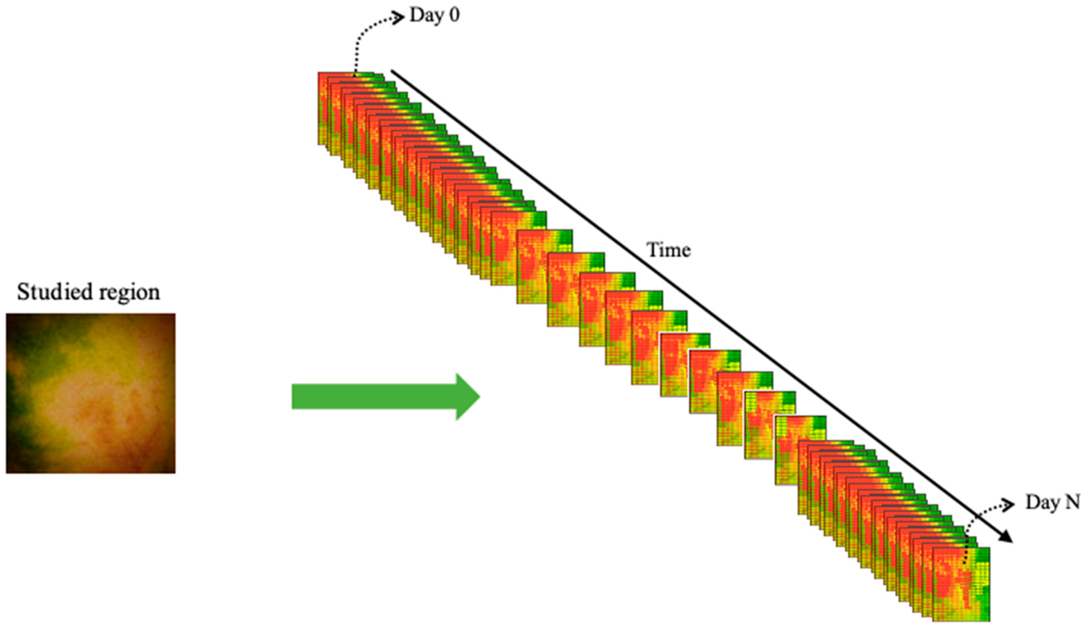
Spatio–temporal rasters can be viewed as a sequence of rasters for the same region and for a defined period of time. Each raster represents information related to the studied region at regular intervals of time (e.g., every second, minute, hour, etc.)—see Figure 2. Spatio–temporal rasters allow the analysis of the gradual evolution of temporal phenomena such as the detection of abnormal phenomenon evolution over time in the studied region.
Spatio–temporal rasters are used in many applications such as climate science to analyze data related to atmospheric and oceanic conditions, which allow us to better understand the Earth’s system. Precision agriculture analyses the different factors impacting the crop yields in order to optimize the production cycle. As mentioned above, in the most real cases, the region of interest can be a sub-region of the raster and not the entire raster, but for the sake of simplification, in this paper, we consider that the sub-region is the entire raster.

2.2.2. Query Spatio–Temporal Raster Data

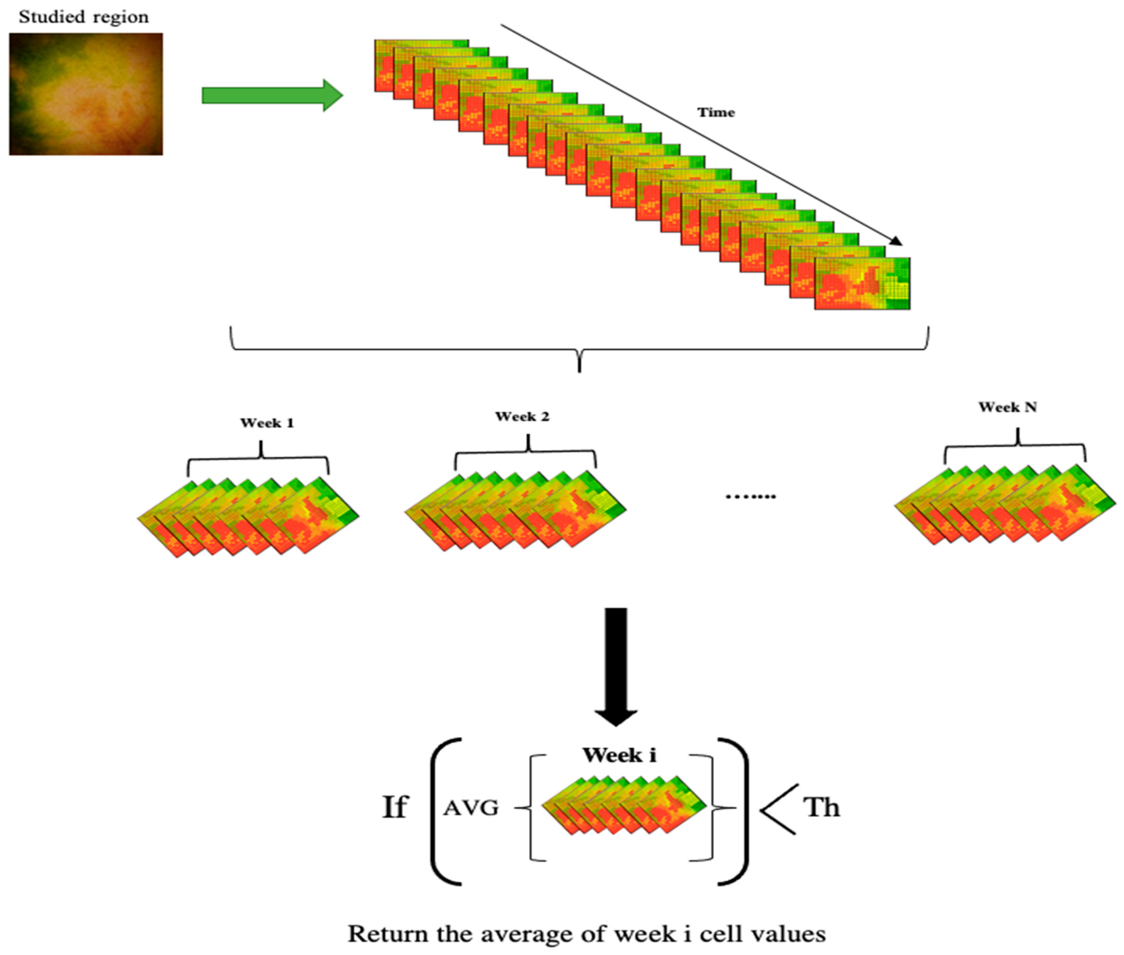
The objective of our query is to provide users with a tool to analyze spatio–temporal rasters measuring a characteristic C (e.g., temperature) collected in a regular time interval (e.g., every hour). More precisely, the query consists of selecting periods of time (subsequences of rasters) where the average of C, over the raster subsequences, is lower than a threshold fixed by the user. For instance, suppose that a scientist wants to know the weeks where the temperature is less than 20 °C. She/he can analyze such a case on an object of study (e.g., a crop in agriculture).
The workflow of the query is presented in Figure 3. It consists of computing a spatio–temporal average of raster cells. A single numerical indicator is returned, i.e., the average of the cells in all the rasters in the studied temporal subsequence (a week).

2.2.3. Heterogenous Computing

In the last decade, HPC (high-performance computing) has seen a significant evolution, because of the emergence of GPU–CPU heterogeneous architectures, which has led to a great revolution in parallel programming. The previous generations of computers contained only central processing units (CPUs) that were dedicated to performing general programming tasks; however, in the last decades, several computers with different architectures have emerged including other processing elements, for instance, GPUs (Graphics Processing Units).
In its beginning, the GPU was a simple device dedicated to graphical processing tasks (i.e., rendering); however, in the last decade, thanks to the industrial success of computer games development, GPUs become powerful tools capable of solving more complicated problems since they are provided with massively parallel programmable processors. A typical heterogeneous architecture is composed of one CPU called the host and one or more GPUs called the device. The communication between the Host and the Device is achieved through the PCI-express bus. The cooperation of the CPU and the GPU led to high-performances and powerful computing capabilities which make the heterogeneous architectures suitable tools for HPC (High Performance Computing). The host code is run on the CPU while the device code is run on the GPU. An application executing on a heterogeneous platform is firstly initialized by the CPU which is responsible for managing the environment, code, and data for the device. In the end, parallel tasks are loaded on the device.

2.2.4. GPU Architecture

The GPGPUs are suitable for data parallelism since they are based on the SIMD paradigm (single instruction multiple data). Therefore, multiple cores perform the same instructions on different parts of the data. Thus, many works have used the GPGPU for several problems, for instance: simulations, image processing, optimizations, etc. The GPGPU device is composed of several SMs (streaming multiprocessor) which are responsible for running the parallel functions called kernels. Each SM contains a set of elements among which include:
  • Registers,
  • Memory caches,
  • Warp schedulers,
  • Execution pipelines.
There are many APIs proposed to exploit the power of the GPGPUs such as OpenCL and CUDA (Compute Unified Device Architecture). This later is a parallel platform and programming model created by NVIDIA to use the GPGPU computing in an efficient and easy way since its syntax is quite similar to C programming. Indeed, NVIDIA uses C with additional specifications expressing the parallelism related to CUDA; however, there are other features which must be mastered and be familiarized, in order to use CUDA properly, such as the programming and memory model.
To execute the CUDA program, three steps are required:
  • Initializing and transferring the data from the Host (CPU) to the Device (GPU),
  • Calling the kernel (parallel function executed on the device by many threads),
  • At the end of the data processing, transferring the results from the Device to the Host.
CUDA provides a specific thread organization which offers the programmer a flexible thread organization. Threads are grouped in blocks which are then grouped in grids [29]. To launch the kernels, we need to specify the size of the grids and the blocks.

2.2.5. GPU-Accelerated Libraries for Computing

NVIDIA GPU-accelerated libraries provide highly optimized functions that can help users to write and optimally scale applications. Using them allows for highly efficient implementations of algorithms that are widely used as building blocks for many applications in several fields and many kinds of libraries are available. There are libraries for linear algebra (cuBLAS and CUDA Math library). For deep learning, there are libraries for parallel algorithms such as Thrust (used for parallel algorithms and data structures). The libraries that interest us in this work are Thrust and CUB since they provide a set of fundamental parallel algorithms that are implemented in an optimized and efficient way, such as reduction and sort, which are used in this work.

Thrust

Developed by NVIDIA, Thrust is a high-level CUDA library that enables the programmers to obtain a high performance and improve their productivity since it is based on the STL (Standard Template Library). The power of Thrust relies on its interoperability with other technologies, for example, C++, Open MP, etc. Additionally, it is a part of the CUDA toolkit.

CUB

CUB is a very fast library founded using the CUDA programming model. It provides state-of-the-art, reusable software components for every layer of the CUDA programming model.
For instance:
  • Device-wide primitives,
  • Block-wide “collective” primitives;
  • Warp-wide “collective” primitives.
Like Thrust, it allows the programmer to obtain a very high performance and efficiency.

3. Query Definition and the Proposed Methods

3.1. Query Formulation

Here, we provide a description of our query.
Let D be the data set (R1, …, RN) of N rasters, where each Ri is a 2D grid that has the size of p × q. All the rasters have the same size and correspond to the same geographical region. Let cellx,y(Ri) be the cell in the raster Ri, and (x, y) be the coordinates of the cell in the raster. The query relies on: Finding all the disjoint (i.e., non-overlapping) raster subsequences Sj in D of length L, such that the mean over Sj is less than T. (T is a threshold defined by the user).

3.2. Sequential Method for Query Processing

The serial straightforward method is as follows:
D = list of rasters
N = the number of rasters in D
L = the size of subsequences
T = the threshold chosen by the user
Result = { }
for every Sj in D {
sum_subseq = 0
for every raster Ri in Sj
  {
   avg_raster = the cell average for Ri
   sum_subseq = (sum _subseq +avg_raster)
  }
avg_subseq = (sum_ subseq)/L
if (avg < T)
  then Result = Result { Sj }.
}

3.3. Parallel Methods for Query Processing

In this subsection, we present the different approaches to implement the query based on the GPGPU.

3.3.1. Straightforward Parallel Approach

This approach consists, as the first step, computing the average of each subsequence in D and then verifying if it satisfies the user condition. Concerning this step, we have used the segmented reduction technique with the sum operator. This later is a building block for many algorithms. In general, it relies on reducing data over many irregular-length segments. In our case, the segments have the same length which is the size of the subsequences L.
In our method, the rasters are aligned and stored in one array. The segments are composed of the cells of all the rasters belonging to them. To perform the segmented reduction, one unique key is assigned to each segment and therefore to each subsequence in our array. If there are N subsequences of size L, there will be N fixed-size segments.
This approach allows for performing the reduction on all the subsequences only once (based on their keys). Hence the function (kernel) responsible for the reduction is called just once on the array containing the data. The output will be a single 1D array containing the means of all the subsequences Sj. An illustrative example is presented below with six rasters: Ijgi 10 00816 i001
Rasters are aligned and stored in one array as follow: Ijgi 10 00816 i002
Our query allows for selecting subsequences of size L such that the average over these subsequences satisfies the user’s condition. In our example L = 3 (3 rasters): Ijgi 10 00816 i003
Now, the same key is assigned to each cell in the same subsequence. Hence, we obtain two segments and the sum of each subsequence is computed based on their keys. Ijgi 10 00816 i004
Concerning the second step which consists of testing if the average of each subsequence Sj is satisfying the user’s condition, we assign one thread to each result in the output array which will be responsible for checking the condition.
The straightforward parallel approach is quite simple since the segmented reduction function is called only once. After that, threads are launched to check the user’s threshold condition; however, the main limitation of this straightforward approach is that the reduction operation is very expensive in time and computation.

3.3.2. Improved Parallel Approach

Based on a Sort

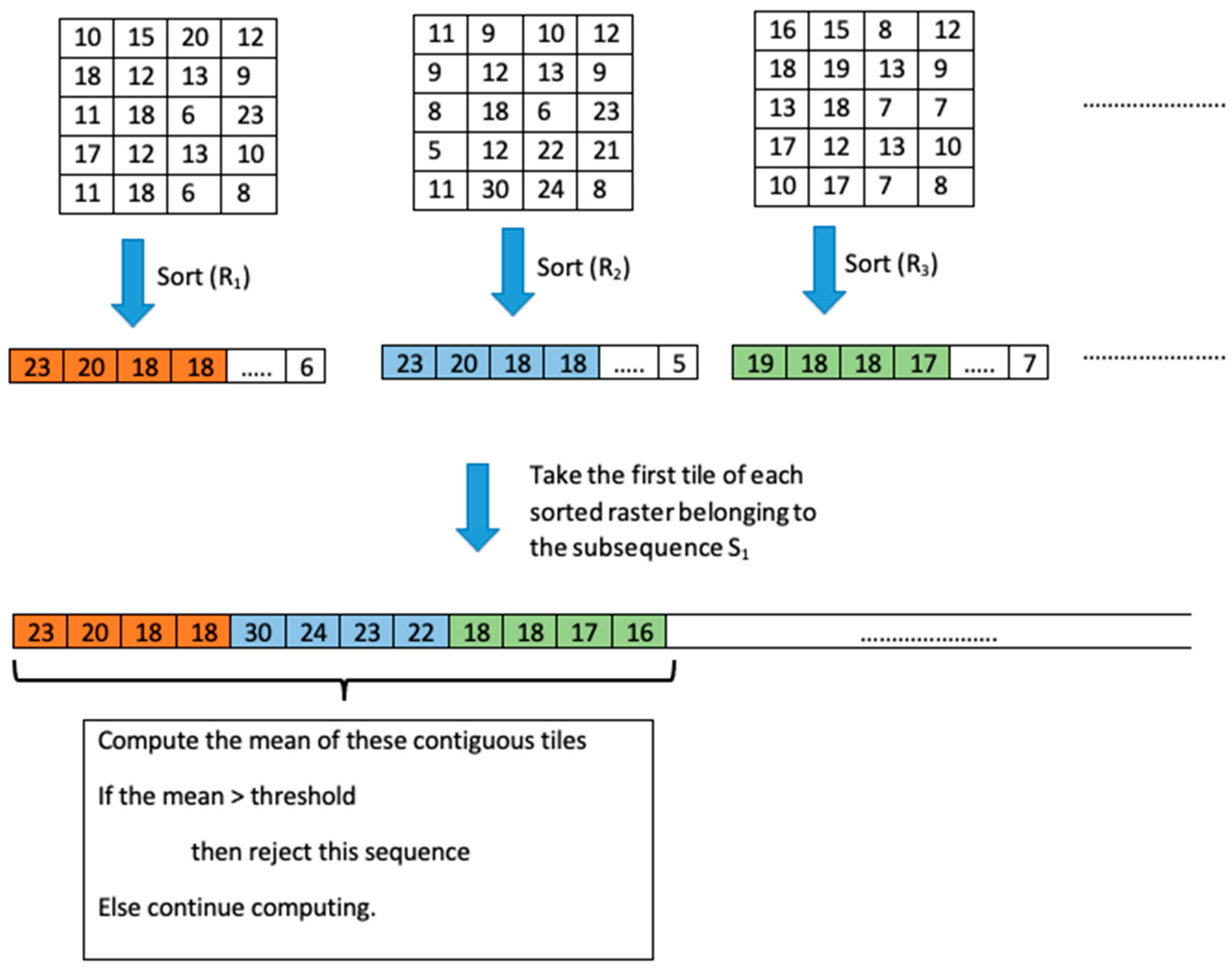
In this subsection, we overcome the limitation of the straightforward parallel approach by introducing a sorting step in the process. We have introduced the main principle for the individual selection of rasters in [8,28]. The idea behind the sorting is to try to reject the subsequences not satisfying the query condition in the early stages to avoid useless computations, since the goal of the query is not to compute the average of all subsequences. We do not have to complete the average computation for a subsequence that does not satisfy the condition. A subsequence average computation can be stopped as soon as we are sure that the user-defined condition will not be satisfied. As a first step, we propose to sort the cells of each raster in descending order. In that case, the threshold is reached faster for the subsequence Sj that does not satisfy the user-defined threshold.
As we can see in Figure 4, the first step consists in sorting all the rasters in parallel and descending order. To do that efficiently and optimally we have adopted the segmented-sort parallel technique to ensure all rasters are sorted in one shot. To achieve this objective, we have chosen a data parallel primitive approach, for instance the cub::DeviceSegmentedRadixSort parallel primitive function which allows the performing of a batched radix sort across multiple, non-overlapping sequences. The reason why we decided to use these parallel primitives was to reduce the implementation complexity and maximize the performance of our algorithms, since these parallel primitives are highly optimized.
Once the rasters are sorted, we move to the second step and it consists of splitting each sorted raster into equal segments (tiles). Thus, the first tile of each raster contains the cells of the largest numbers. We consider the positive numbers for cell values. In the case of negative numbers in the datasets, shifting by a large number is needed (e.g., adding 100 to all the values).
In the first iteration, we compute only the sum of the first tiles of each raster for a given subsequence Sj. If the result Res1 is not satisfying the query condition, then the subsequence Sj is rejected. Otherwise, we repeat the same processing for the second tiles of each raster in Sj, add it to Res1(the previous results of the first segments) and check the results. If the Res2 is not satisfying the query condition then Sj is rejected. Otherwise, we repeat the process for the third segment of rasters in Sj and so on. This will be done in parallel at the same time for all the disjoint subsequences.
The main drawback of this approach is that the sorting process is expensive in time and computations, especially in the case of large rasters. To overcome this limitation, we propose in the next subsection avoiding sorting all the rasters and settling for sorting only a few of them. The others will be somehow reordered according to the sorted rasters. This is the subject of the next subsection.
In our example, we consider that the user condition is “the mean must be less than a threshold”. Note that if the user-defined condition would be “the mean must be greater than a threshold”, the operation in Figure 5 will be “if the mean > threshold then accept this sequence”.

Based on the Sophisticated Sort

We consider that we do not know in advance on which datasets the query will be applied as the data set can change from one query to another. We take the point of view of a database management system (DBMS) designer and the goal is to implement generic DBMS operations. Our goal is not to improve the computation for a particular data set. Sorting is expensive, i.e., the time complexity of a sort is O(n log n) in the case of quicksort, and is higher than the sum computation, i.e., O(n). In practice, the sorting cannot be a pre-processing step of all the rasters of the whole data set before the query execution, because this process is too time-consuming and the dataset used for a query will not necessarily be reused for later queries. We propose to execute the sorting at the query runtime on only some rasters. More precisely, we propose the following:
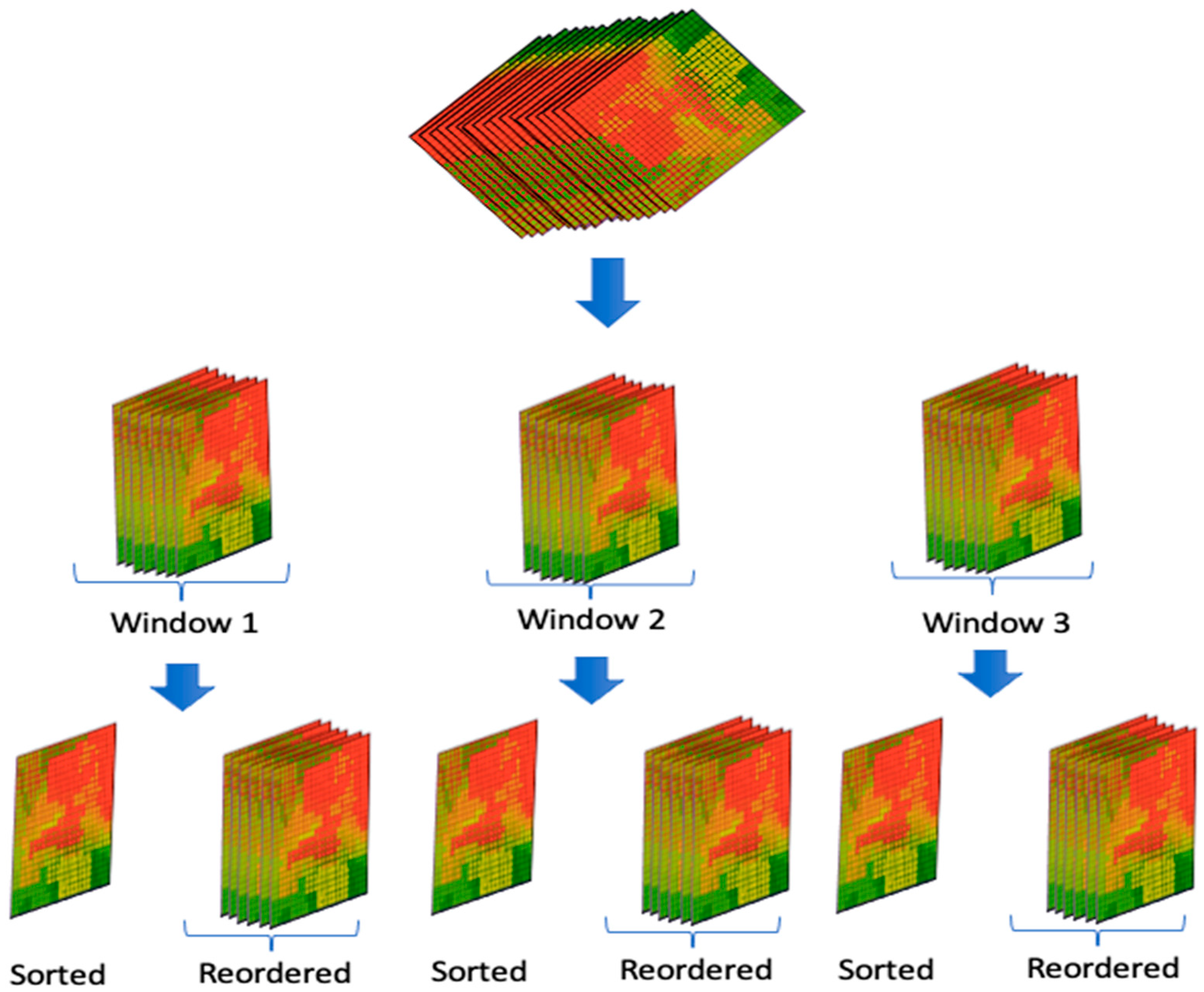
  • Split the dataset of our rasters in time windows containing a fixed number of rasters. Thus, we propose to sort only one raster from each time window. The sorting result can be viewed as an array M mapping a cell position (x, y) to an order position I.
  • The cells of rasters falling in the same time window will be reordered based on the sorted raster of this time window. To do this, the array M will be directly used during the average computation without an impact on time complexity. The time window can be the size of the subsequences.
Figure 5 illustrates this approach. As we can see in this figure, the data sets are divided in three-time windows of a fixed size 7. In the second step, for each segment, one raster is sorted and the rest are reordered accordingly. This strategy allows us to avoid the heavy computations of sorting all the rasters. We propose to sort only a few among them which gives us the possibility to reduce the processing time of the sorting step.
The idea behind this method is that in many phenomena the spatial distribution of values evaluates rather slowly over time. Therefore, we suppose that the rasters that are falling in a certain window of time have the same behavior in term of the cell values. For example, if the rasters represent the hourly temperature of a specific region, the main spatial distribution of temperature will not change or will make only a slight change during a certain period of time (window), so the rasters that fall in the same time window have the same behavior. Thus, we need to sort only one raster from each window and reorder the others accordingly.
In practice, performance improvement depends on two things:
  • The size of the time window—which must not be too large and also not too small. If it is too large, the difference between the estimated cell sorting and the real cell sorting may increase inside the time window. Hence the performance may drop (the sort becomes useless). If the time window size is too small, the number of the sorted rasters will increase in the global processing and it will slow down the execution time.
  • The type of data (the temperature, pressure, etc.). The less the data is evolving over time the more the sorting is accurate. The proposed methods perform better when the spatial locations of maximal and minimal values evolve slowly over time.
To implement that, first we sorted the indexes (keys) of the rasters that must be sorted. We used the sorted keys to reorder the other rasters. To sort the raster and indexes, two solutions are available: the solution based on CUB with cub::DeviceRadixSort::SortPairs, and the solution based on Thrust with thrust::sort_by_key. The other rasters that fell in the same time windows were reordered (sorted) according to the sorted raster using the gather transformation that could be implemented using the primitive thrust::gather. Once the rasters were sorted, we needed to implement the kernel responsible for computing the average of the subsequences using our method described above. To do that, the primitives thrust::reduce or the cub::DeviceReduce::Reduce could be used.

4. Tests and Analysis

4.1. Configuration of the Experimental Environment

Our experiments were performed on two platforms. Concerning the parallel methods, we have used a GPU-based platform: Tesla K20 C, while the sequential approaches were performed on Intel(R) Core(TM). To implement our methods we have used C++, CUDA and the libraries Thrust and CUB.
Table 1 shows the details related to the used hardware and software configuration.
In the tests, we aimed to outline the power of using the GPGPU platform to speed up the spatio–temporal raster queries over the classical approaches based on the CPU. Besides this, we showed that based on the type and the distribution of data in our dataset, we could gain more performance by using the sort heuristic presented above.

4.2. Dataset

4.2.1. INRAE Montoldre Site

In our experiments, we used a dataset provided by the INRAE Montoldre site [30,31], which is a large experimental farm located in Montoldre. This was later dedicated to the development and the experimentation of agri-environmental techniques. Based on a sensor network composed by LiveNode [32] (developed by LIMOS), this platform provides real data that are used by researchers in their work related to the environment. The measurements used were air and soil humidity, temperature and light and they were measured using several sensors distributed over the Montoldre site.
The Montoldre raw dataset produced by LiveNode is composed of two SQL tables, the network table and the sensors table.
  • The network table concerns information about 10 sensor nodes,
  • The sensors table contains columns such as: myNodeID, battery, temperature, humidity, light, etc., and 14,970,995 rows which correspond to the measurements of the different sensors during many months with a different fine-grained frequency of acquisition.
The table below (Table 2) shows the description of some measures.
The inverse distance weighted IDW [33] interpolation method was used for predicting the missing values of the unsampled locations to produce rasters based on the raw INRAE dataset. Hence, 3550 rasters were produced in four different resolutions (300 × 300, 350 × 350, 400 × 400, 450 × 450) for three types of measures (temperature, humidity, watermark 2).
For each type of measurement and each resolution, one raster was generated per hour, with a value between the Min. and Max. (Table 3) available sensor measures—since all the sensors were not always active at the same time.

4.2.2. Statistical Description of the Montoldre Hourly Dataset

Hereunder is a table (Table 3) which shows the statistical description of the datasets such that:
  • Min: is the minimum value of the measure in the whole dataset,
  • Max: is the maximum value of the measure in the whole dataset,
  • Mean: is the mean value of the measure in the whole dataset,
  • Standard deviation: is the standard deviation of the measure in the whole dataset,
  • Mean of rasters means: to compute this value, first we computed the mean of each raster used for our experiments then we computed the global mean which is the mean over the raster means,
  • Mean of rasters standard deviation: to compute this value, first we computed the standard deviation of each raster used for our experiments then we computed the mean over all the standard deviations of the rasters.

4.3. Experiment Results and Analysis

4.3.1. Experiment Results

In this subsection we present the results of our method. As cited before we have used several datasets with three measures: temperature (Table 4), humidity (Table 5), and watermark 2 (Table 6). Hence, we present the results for each measure. To do this, we have generated four datasets and each one contains: 3550 rasters with a different raster size. We have fixed the size of the time windows at 10 and the size of the sequences as equal to 6.
As you can see, hereunder, The Table 4 represents the results on the temperature measure, the Table 5 concerns the air humidity measure, while the Table 6 shows the results using the watermark 2 measure.
As we can see in the results, using the temperature datasets always showed good results for using the GPU over the CPU version; however, our improved method based on the rejection step based on sorting, showed bad results for the CPU-sorting and the GPU-sorting for the temperature dataset. The time of execution was worse compared to the methods without sorting. Our improved methods are based on a sorting step that must allow for rejecting the raster sequences earlier; however, the values of the temperature dataset were too close to each other in the rasters. The mean of rasters standard deviation of temperature was equal to 2.73, which explains the low variation of the values in the temperature rasters data. The goal of the sorting step was to allow for summing the highest values first. Consequently, when the values were too close in the rasters, the sorting step was useless in reaching the threshold quickly and rejecting rasters in an earlier stage. In this case, the sorting step became a heavy burden on the method, since sorting is expensive in term of computations. Hence the execution time was higher than the methods without sorting.
Concerning the humidity and watermark 2 datasets, the GPU-based methods were always better than the CPU methods (Table 5 and Table 6); however, unlike the previous results based on the temperature dataset, our methods using the sorting step enhanced the results of the parallel version. This is due to the sorting step which allowed for rejecting raster sequences in earlier stages, because of the distribution of the humidity and watermark data values. The mean of rasters standard deviation of the humidity dataset was equal to 15.20, and 43.79 for the watermark 2 dataset (Table 3).
As a summary, our methods without sorting based on the GPU give good results compared to the CPU over all the datasets and the measures however, when the dataset has a high variation of values such as for humidity and watermark 2, using our methods based on sorting can improve the results, since it allows us to reject data not satisfying the user condition in the early stages. When data has a low variation of values, the method based on sorting must be avoided.

4.3.2. The Impact of the Time Window Size on the Performance

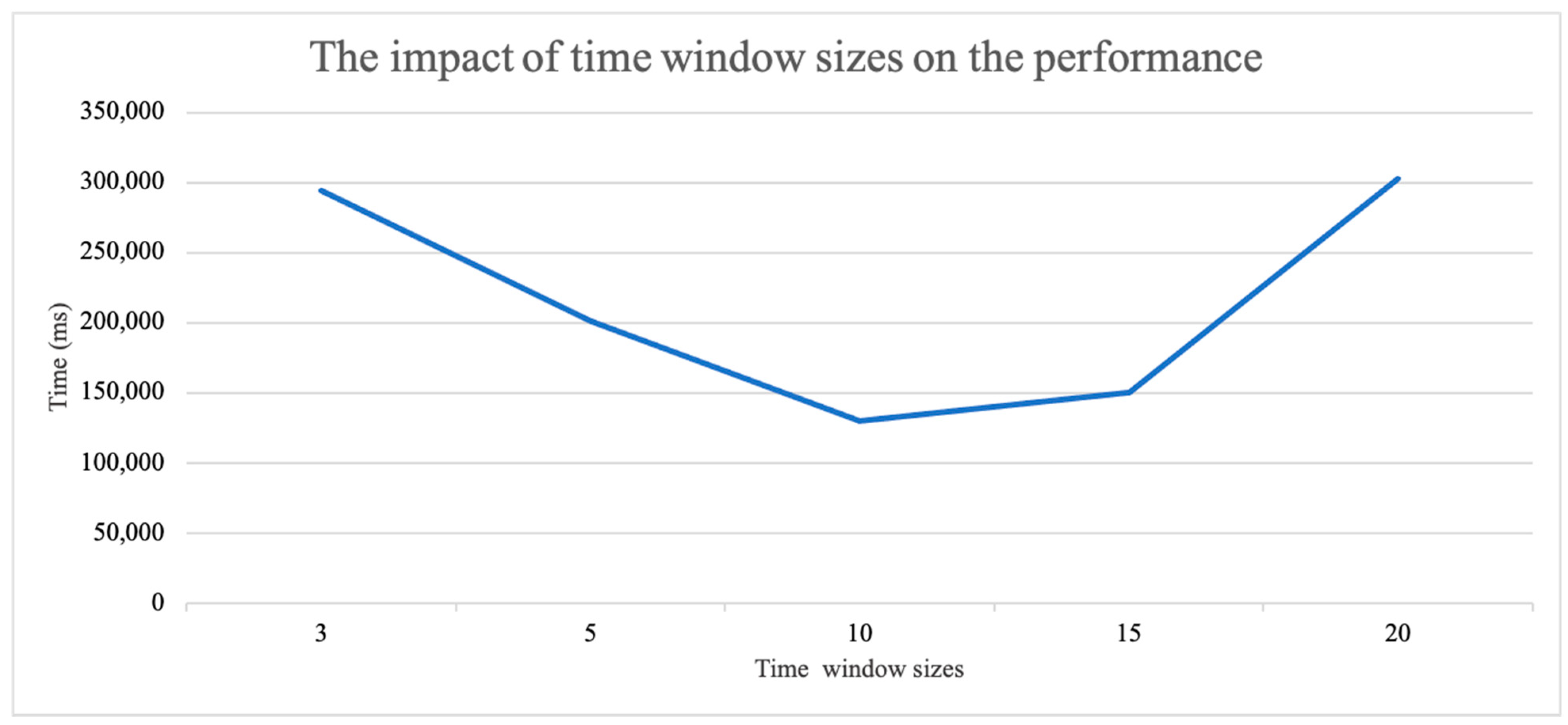
Here we show how the time window size impacts the performance over “dataset 4” for the watermark 2 measurement using the same fixed parameters cited above. As we can see in Figure 6, when the time window size is too small (size = 3), the number of time windows increases as well as the number of sorted rasters. Since the sorting is expensive, this will increase the time execution. On the contrary, when the time window size is too large (size = 20), it will impact the reordering precision of the rasters and hence the sorting becomes useless which will lead to a performance drop; however, when the time window is not too small and not too large (size = 10), we obtain a good performance.

5. Conclusions and Future Work

Processing large-scale spatio–temporal data is experiencing an increasing importance and is required by many fields among which is included precision agriculture. Analyzing these data, for instance, weather, soil humidity, etc., allows for extracting more valuable, crucial and accurate information required to analyze environmental phenomena.
The main requirement for spatial data-intensive applications is the processing time and scalability. Unfortunately, most of the existing methods are based on traditional approaches and are not appropriate for querying massive spatial data efficiently.
In this paper, we addressed the problem of speeding up the spatio–temporal rasters data-based query consisting of selecting only disjoint raster subsequences of a fixed size, such that the average of the cells over these subsequences is less than a user defined threshold.
In recent years, several big raster spatio–temporal data processing infrastructures have been developed for information mining. For instance, XArray [34], which is an efficient tool for processing scientific datasets and widely used by the GIS community for processing raster spatial data. Fully integrated in DASK [35], it allows the processing of big raster data.
Despite their simplicity and their efficiency, most of these solutions are based on high level languages, e.g., Python, and provide high level pre-built functions which make them slower and without the high flexibility to implement very bespoke algorithms.
In this paper, we are working on a very specific query which is not yet implemented in the existing raster data processing systems. Our goal is to propose a generic and very fast solution and this can be achieved only by using low level programming languages (e.g., C++). Moreover, their flexibility allows us to include a heuristic based on sorting in order to save computations, remembering that our problem belongs to massive data computations which are very suitable for a GPU parallel, which justifies our solution.
Thus, in our work, first we have shown that we can improve the processing of the said query by using the power of recent GPU devices. Furthermore, using parallel primitives based on CUDA allowed us to further optimize our implementation and reduce the coding complexity. Second, we have designed and implemented a new method based on a sort process to avoid useless computations and hence further accelerated the processing time of our query. The proposed approaches have been tested on the real dataset provided by the INRAE experiment farm using three measures: temperature, humidity and watermark 2, that are essential for agriculture.
The experimental results on temperature show that our method without sorting based on the GPU performs better than the CPU over all the datasets; however, the methods (CPU and GPU) based on sorting show poor results (The time of execution is worse compared to the methods without sorting). As cited above, this is due to the nature of the temperature data (mean of rasters standard deviation = 2.73).
Concerning the air humidity and watermark 2 measures, the experimental results have shown that GPU-based methods are always better than the CPU methods over all the datasets. Furthermore, our methods using the sorting step enhance the results, especially, for the parallel version. Thus, a significant speed up is obtained (4,8) for the dataset 4 for watermark 2 and humidity.
As mentioned above, our optimized method based on sorting is sensitive to data distribution; it works only in the case of high variations in data (e.g., in our case humidity and watermark 2) and it does not work in the case of data with low variations such as temperature.
We have to highlight that our method based on sorting is not limited to spatial data but it can be used in other applications which use the same form and characteristics of data. Furthermore, the query can be extended to other operations besides the average, for example, min. or max. and the user can also change the constraint.
As future work, we would like to predict mathematically the optimal size of the time window and the size of the tiles, as this will help to avoid the empirical method which is a time consuming and imprecise method for choosing the best values for tile and time window sizes. Furthermore, we want to provide more precise statical parameters for the dataset description in order to provide a decision-making support for either using the sorting-based method or remaining content with the GPU-based method without sorting. Additionally, the investigation of the use of our methods (for instance, the rejection process based on sorting) on other fields will be very useful in order to study the behavior of our methods on other types of data from other fields and applications. The proposed GPGPU-based sorting method to improve raster selection performance is currently not implemented in traditional libraries such as spatial XArray [34]. The proposed improvement is generic and can be integrated in such libraries.
A future work can include implementing the proposed method (with sorting) in this manuscript as an XArray module and compared with an XArray-based method (without sorting).
Finally, we would like to expand the use of the power of the GPU for more massive computations and complex queries, and running our methods on different heterogeneous computing solutions such as OpenCL, which will be very useful for making a complete comparison between all the solutions.

Author Contributions

Supervision, F.P. and M.-A.K.; writing—original draft, D.E.-N.; writing—review and editing, D.E.-N., F.P. and M.-A.K. All authors have read and agreed to the published version of the manuscript.

Funding

This work was funded by grants from the French program “investissement d’Avenir” managed by the Agence Nationale de la Recherche of the French government (ANR), the European Commission (Auvergne FEDER funds) and” Région Auvergne” in the framework of LabEx IMobS 3 (ANR-10- LABX-16-01).

Acknowledgments

We acknowledge the support received from the Agence Nationale de la Recherche of the French government through the program “Investissements d’Avenir” 16-IDEX-0001 CAP 20-25 on the general topic of this paper. Also, we would like to thank all the members of LIMOS (UCA) and the COPAIN team (INRAE) involved in the deployment of the LiveNode network in INRAE Montoldre and in the collection and documentation of data.

Conflicts of Interest

The authors declare no conflict of interest.

References

  1. Sawant, S.; Durbha, S.S.; Jagarlapudi, A. Interoperable agro-meteorological observation and analysis platform for precision agriculture: A case study in citrus crop water requirement estimation. Comput. Electron. Agric. 2017, 138, 175–187. [Google Scholar] [CrossRef]
  2. Pinet, F. Entity-relationship and object-oriented formalisms for modeling spatial environmental data. Environ. Model. Softw. 2012, 30, 80–91. [Google Scholar] [CrossRef]
  3. Laurini, R.; Thompson, D. 6—Tessellations: Regular and Irregular Cells, Hierarchies. In Fundamentals of Spatial Information Systems; Laurini, R., Thompson, D., Eds.; Academic Press: Cambridge, MA, USA, 1992; pp. 217–256. ISBN 9780124383807. [Google Scholar] [CrossRef]
  4. Kang, M.A.; Zaamoune, M.; Pinet, F.; Bimonte, S.; Beaune, P. Optimisation des performances des opérations d’agrégation au sein des entrepôts de grilles spatialisées (in French). In Proceedings of the SAGEO 2013 Conférence Internationale de Géomatique et d’analyse Spatiale, Brest, France, 26 September 2013. [Google Scholar]
  5. Kang, M.-A.; Zaamoune, M.; Pinet, F.; Bimonte, S.; Beaune, P. Performance optimization of grid aggregation in spatial data warehouses. Int. J. Digit. Earth 2015, 8, 970–988. [Google Scholar] [CrossRef]
  6. Pullar, D. MapScript: A Map Algebra Programming Language Incorporating Neighborhood Analysis. GeoInformatica 2001, 5, 145–163. [Google Scholar] [CrossRef]
  7. Tomlin, C.D. Map algebra: One perspective. Landsc. Urban Plan. 1994, 30, 3–12. [Google Scholar] [CrossRef]
  8. En-Nejjary, D.; Pinet, F.; Kang, M.-A. A Method to Improve the Performance of Raster Selection Based on a User-Defined Condition: An Example of Application for Agri-environmental Data. Adv. Intell. Syst. Comput. 2018, 893, 190–201. [Google Scholar]
  9. En-Nejjary, D.; Pinet, F.; Kang, M. Modeling and Computing Overlapping Aggregation of Large Data Sequences in Geographic Information Systems. Int. J. Inf. Syst. Modeling Des. 2019, 10, 20–41. [Google Scholar] [CrossRef]
  10. Thrust. Available online: https://thrust.github.io (accessed on 28 November 2021).
  11. CUB. Available online: https://nvlabs.github.io/cub (accessed on 28 November 2021).
  12. Viola, I.; Kanitsar, A.; Groller, M.E. Hardware-based nonlinear filtering and segmentation using high-level shading languages. In Proceedings of the the IEEE Visualization 2003, Seattle, WA, USA, 19–24 October 2003; pp. 309–316. [Google Scholar] [CrossRef]
  13. Yang, Z.; Zhu, Y.; Pu, Y. Parallel Image Processing Based on CUDA. In Proceedings of the the 2008 International Conference on Computer Science and Software Engineering, Wuhan, China, 12–14 December 2008; pp. 198–201. [Google Scholar] [CrossRef]
  14. Temizel, A.; Halici, T.; Logoglu, B.; Temizel, T.T.; Omruuzun, F.; Karaman, E. Experiences on image and video processing with CUDA and OpenCL. In GPU Computing Gems; Morgan Kaufmann: Boston, MA, USA, 2011; pp. 547–567. [Google Scholar]
  15. Jain, P.; Mo, X.; Jain, A.; Subbaraj, H.; Durrani, R.S.; Tumanov, A.; Gonzalez, J.; Stoica, I. Dynamic Space-Time Scheduling for GPU Inference. arXiv 2018, arXiv:1901.00041. [Google Scholar]
  16. Jianbo, Z.; Wenxin, Y.; Jing, S.; Yonghong, L. GPU-accelerated parallel algorithms for map algebra. In Proceedings of the the 2010 The 2nd Conference on Environmental Science and Information Application Technology, Wuhan, China, 17–18 July 2010; pp. 882–885. [Google Scholar] [CrossRef]
  17. Jianting, Z.; Simin, Y.; Le, G. Large-scale spatial data processing on GPUs and GPU-accelerated clusters. Sigspatial Spec. 2015, 6, 27–34. [Google Scholar] [CrossRef] [Green Version]
  18. Steinbach, M.; Hemmerling, R. Accelerating batch processing of spatial raster analysis using GPU. Comput. Geosci. 2012, 45, 212–220. [Google Scholar] [CrossRef]
  19. Zhang, J.; You, S.; Gruenwald, L. Parallel online spatial and temporal aggregations on multi-core CPUs and many-core GPUs. Inf. Syst. 2014, 44, 134–154. [Google Scholar] [CrossRef]
  20. Jianting, Z.; Simin, Y. High-performance quadtree constructions on large-scale geospatial rasters using GPGPU parallel primitives. Int. J. Geogr. Inf. Sci. 2013, 27, 2207–2226. [Google Scholar] [CrossRef]
  21. Doraiswamy, H.; Freire, J. A GPU-friendly Geometric Data Model and Algebra for Spatial Queries. In Proceedings of the ACM SIGMOD International Conference on Management of Data, SIGMOD ’20, Portland, OR, USA, 14–19 June 2020; pp. 1875–1885. [Google Scholar] [CrossRef]
  22. Doraiswamy, H.; Vo, H.T.; Silva, C.T.; Freire, J. A GPU-based index to support interactive spatio-temporal queries over historical data. In Proceedings of the 2016 IEEE 32nd International Conference on Data Engineering, ICDE, Helsinki, Finland, 16–20 May 2016; pp. 1086–1097. [Google Scholar] [CrossRef]
  23. MongoDB. Available online: http://www.mongodb.org (accessed on 28 November 2021).
  24. Beutel, A.; Mølhave, T.; Agarwal, P.K. Natural Neighbor Interpolation Based Grid DEM Construction Using a GPU. In Proceedings of the 18th SIGSPATIAL International Conference on Advances in Geographic Information Systems, San Jose, CA, USA, 2–5 November 2010; pp. 172–181. [Google Scholar] [CrossRef] [Green Version]
  25. Simion, B.; Ray, S.; Brown, A.D. Speeding up Spatial Database Query Execution using GPUs. Procedia Comput. Sci. 2012, 9, 1870–1879. [Google Scholar] [CrossRef] [Green Version]
  26. Walsh, S.D.C.; Saar, M.; Bailey, P.; Lilja, D. Accelerating geoscience and engineering system simulations on graphics hardware. Comput. Geosci. 2009, 35, 2353–2364. [Google Scholar] [CrossRef]
  27. Wu, Y.; Ge, Y.; Yan, W.; Li, X. Improving the performance of spatial raster analysis in GIS using GPU. In Proceedings of the SPIE-The International Society for Optical Engineering, Nanjing, China, 7 August 2007. [Google Scholar]
  28. En-Nejjary, D.; Pinet, F.; Kang, M. Large-scale geo-spatial raster selection method based on a User-defined condition using GPGPU. In Proceedings of the 11th International Conference on Computer Science and Information Technology, Paris, France, 21–23 December 2018; p. 8. [Google Scholar]
  29. Cheng, J.; Grossman, M.; McKercher, T. Professional CUDA C Programming; John Wiley & Sons: Hoboken, NJ, USA, 2014. [Google Scholar]
  30. Roussey, C.; Bernard, S.; André, G.; Boffety, D. Weather data publication on the LOD using SOSA/SSN ontology. Semant. Web 2020, 11, 581–591. [Google Scholar] [CrossRef]
  31. Touseau, L.; Le Sommer, N.L. Contribution of the web of things and of the opportunistic computing to the smart agriculture: A practical experiment. Future Internet 2019, 11, 33. [Google Scholar] [CrossRef] [Green Version]
  32. Hou, K.M.; de Sousa, G.; Chanet, J.P.; Zhou, H.Y.; Kara, M.; Amamra, A.; Diao, X.; de Vaulx, C.; Li, J.J.; Jacquot, A. LiveNode: LIMOS versatile embedded wireless sensor node. In Proceedings of the Workshop International sur Les Réseaux de Capteurs sans Fil en Conjonction avec la 7ème Conférence Internationale sur les NOuvelles TEchnologies de la REpartition (NOTERE), Marrakech, Marrakech, 4 June 2007; p. 5. [Google Scholar]
  33. Li, Z.; Wang, K.; Ma, H.; Wu, Y. An Adjusted Inverse Distance Weighted Spatial Interpolation Method. In Proceedings of the 2018 3rd International Conference on Communications, Information Management and Network Security (CIMNS 2018), Wuhan, China, 27–28 September 2018; pp. 128–132. [Google Scholar] [CrossRef] [Green Version]
  34. Hoyer, S.; Hamman, J. xarray: N-D labeled Arrays and Datasets in Python. J. Open Res. Softw. 2017, 5, 10. [Google Scholar] [CrossRef] [Green Version]
  35. Dask Development Team. Dask: Library for Dynamic Task Scheduling. 2016. Available online: https://dask.org (accessed on 25 November 2021).
Figure 1. A raster is composed of rows and columns of cells.
Ijgi 10 00816 g001
Figure 2. Spatio–temporal rasters representing the evolution of the temperature during N days for a studied region.
Ijgi 10 00816 g002
Figure 3. Overall framework for the query process.
Ijgi 10 00816 g003
Figure 4. Illustration of our method for the first subsequence S1.
Ijgi 10 00816 g004
Figure 5. Strategy to avoid sorting all the rasters.
Ijgi 10 00816 g005
Figure 6. The time windows’ sizes impact on the performance over the dataset 4.
Ijgi 10 00816 g006
Table 1. Hardware and software configurations.
PlatformHardware ConfigurationSoftware Configuration
CPUIntel(R) Core(TM) i7-2600K
CPU @ 3.40 GHz
Device global memory: 16 GB
Cache size: 20,480 KB
Linux Ubuntu 19.04
C/C++
CUDA 8.0
Thrust v10.1.105
CUB v1.8.0
GPUTesla K20C
CUDA Cores: 2496
Device global memory: 5 GB
Memory Bandwidth: 208 GB/s
Table 2. Description of the measures.
MeasureMeaningUnits
BatteryBattery state of nodemV
TemperatureTemperature measurementC degree
HumidityAir humidity measurementPercent
LightLight measurementN/A
Watermark nMeasurement value of the
n-th watermark device. Watermark is a soil humidity sensor. The Watermark sensors are in the soil at different soil depth.
Watermark’s unit (range: 0 to 200)
Note: Watermark1: this sensor is deployed at 10 cm depth in the soil; watermark 2: this sensor is deployed at 20 cm depth in the soil; watermark3: this sensor is deployed at 30 cm depth in the soil.
Table 3. Statistical description of the dataset.
MeasureMinMaxMeanStandard DeviationMean of Rasters MeansMean of Rasters Standard Deviation
Temperature (°C)045.711.898.73122.73
Humidity
(%)
9.91007821.9778.1515.20
Watermark 2
(watermark’s unit)
120063.8088.9661.7143.79
Table 4. Experiments on Temperature.
DatasetSize of RastersCPU (ms)Sophisticated CPU-Sorting (ms)GPU (ms)Sophisticated GPU-Sorting (ms)
Dataset 1100 × 10025,46434,18021,02329,117
Dataset 2200 × 200240,255380,521190,762316,284
Dataset 31000 × 100349,654471,290260,273397,641
Dataset 4500 × 500587,323697,138418,012631,540
Table 5. Experiments on Air Humidity.
DatasetSize of RastersCPU (ms)GPU (ms)Sophisticated GPU-Sorting (ms)
Dataset 1100 × 10028,23117,3287133
Dataset 2200 × 200250,165131,57161,604
Dataset 31000 × 100369,719171,80383,251
Dataset 4500 × 500608,413372,631127,679
Table 6. Experiments on Watermark 2.
DatasetSize of RastersCPU (ms)GPU (ms)Sophisticated
GPU-Sorting (ms)
Dataset 1100 × 10027,64712,9817276
Dataset 2200 × 200266,499116,73063,452
Dataset 31000 × 100382,122162,01484,916
Dataset 4500 × 500625,116302,833130,233
Publisher’s Note: MDPI stays neutral with regard to jurisdictional claims in published maps and institutional affiliations.