Efficient Group K Nearest-Neighbor Spatial Query Processing in Apache Spark

Abstract

Aiming at the problem of spatial query processing in distributed computing systems, the design and implementation of new distributed spatial query algorithms is a current challenge. Apache Spark is a memory-based framework suitable for real-time and batch processing. Spark-based systems allow users to work on distributed in-memory data, without worrying about the data distribution mechanism and fault-tolerance. Given two datasets of points (called Query and Training), the group K nearest-neighbor (GKNN) query retrieves (K) points of the Training with the smallest sum of distances to every point of the Query. This spatial query has been actively studied in centralized environments and several performance improving techniques and pruning heuristics have been also proposed, while, a distributed algorithm in Apache Hadoop was recently proposed by our team. Since, in general, Apache Hadoop exhibits lower performance than Spark, in this paper, we present the first distributed GKNN query algorithm in Apache Spark and compare it against the one in Apache Hadoop. This algorithm incorporates programming features and facilities that are specific to Apache Spark. Moreover, techniques that improve performance and are applicable in Apache Spark are also incorporated. The results of an extensive set of experiments with real-world spatial datasets are presented, demonstrating that our Apache Spark GKNN solution, with its improvements, is efficient and a clear winner in comparison to processing this query in Apache Hadoop.

1. Introduction

Nowadays, a huge amount of spatial data is generated daily from GPS-enabled devices, such as smart phones, smart watches, cars, sensors, location-tagged posts in Facebook, Instagram, etc. The term big spatial data is related to the process of capturing, storing, managing, analyzing, and visualizing huge amounts of spatial data, not using traditional tools and systems. How to process such big spatial data efficiently has become one of the current research hotspots. To carry out this target, distributed computing using shared-nothing clusters on extreme-scale data has become a dominating trend in the context of data processing and analysis.

Hadoop MapReduce [1] and Apache Spark [2] are the dominating distributed frameworks for processing and managing big data on a cluster of computers. MapReduce is a disk-based distributed framework more suitable for batch processing and not suitable for iterative processing. Apache Spark is a memory-based framework suitable for real-time and batch processing. Following these two distributed frameworks, two types of research prototype systems to manage large-scale spatial data query processing have emerged. One is the Hadoop-based prototype systems, where SpatialHadoop [3] is the most representative system to manage efficiently massive spatial datasets stored on disk. The other type is Spark-based prototype systems, where Sedona (formerly GeoSpark [4]) is actively under development and several companies are currently using it, because it is very efficient to manage spatial datasets that can all fit into main memory. These research prototype systems provide some basic spatial query operations for big spatial data, such as spatial join, range query and other common spatial operators, but they do not provide more specific spatial queries.

The Group (K) Nearest-Neighbor (GKNN) query [5] belongs to the big family of nearest-neighbor searches [6], which has been widely studied in computer science and has numerous modern applications, such as GIS [7], mobile computing [8], clustering [9], outlier detection [10], facilities management [5], etc. Between two datasets of points, the GKNN query retrieves the K points of one dataset (called Training) with the smallest sum of distances to every point of the other dataset (called Query). The Training dataset is considered a static dataset queried by multiple Query datasets. As an example, consider a group of friends (Query points) residing in different areas of a city, arranging for a meeting to a public place (Training point), e.g., restaurant, or pub. They would make a list of K such places with the smallest sum of distances to all friends (as a group) and then choose among these places the one that best suits most of them. Such an example can be constructed for several similar problems. For instance, consider a conference organizing company that wants to find the building location (where the conference could be organized), minimizing the sum of distances (displacement) of all possible assistants to the conference. Another example could be to consider a supermarket chain that wants to find the warehouse location, minimizing the sum of distances to all stores served by the new warehouse. Finally, another application case could be related to a franchise that wants to open a restaurant in order to attract the maximum number of customers from a set of urban areas. A GNNQ reports the restaurant location that minimizes the sum of distances to all urban areas. The evolution of mobile devices, the WWW and sensors create an explosion of data and more applications based on larger datasets, which will require this query to rise.

Without effective pruning and calculation techniques, this query can be very demanding (time consuming) because it involves distance calculations that may be in the order of millions or more. The GKNN query has been actively studied in centralized environments; several performance improving techniques and pruning heuristics have also been proposed and used ([5,7,11,12]). Our recent research works [13,14] are based on the MapReduce programming framework to solve this query in parallel. We have proposed and studied the first algorithm for the GKNN query in Hadoop [13]. This algorithm was significantly improved and implemented in Hadoop and SpatialHadoop [14]. Since Hadoop is a general purpose (not spatially oriented) distributed system, in this paper, we present the first algorithm for this important and demanding query, in another, general purpose and popular distributed system, Apache Spark. In general, Spark is considered more efficient than Hadoop. Examining the performance of these two widely used systems for processing a demanding query like the GKNN, one further highlights their relative efficiency.

More specifically, our contribution in this paper is summarized as follows.

• We present the first Apache Spark based algorithm for the GKNN query, which is based on the MapReduce algorithm of [13,14], suitably modified to take advantage of Spark specific features.
• We present improvements of this algorithm, based on specific functionalities of the Spark framework.
• We extensively compare the new algorithm against the best Hadoop based algorithm of [14], using big real and synthetic datasets.
• Using synthetic datasets, we experimentally study the scalability of the Spark-based algorithm and the effect of each of its embedded improvements on performance.

The work presented in this paper is the first step for the development of a GKNN algorithm in a spatially enabled Spark-based system, such as Sedona [4], since extending such a system with more useful spatial operators, processed by efficient algorithms is important for exploiting its potential in emerging big-data applications.

The rest of this paper is organized as follows. Section 2 reviews spatial query processing in Spark and distributed GKNN query processing. In Section 3, we present the formal definition of the GKNN query and the basic features of Spark. Section 4 follows, where we present in detail the new algorithm for processing the GKNN query in Spark, while in Section 6, we present the improvements of this algorithm. Next, in Section 7, we present the experimentation we performed and the results we obtained, while in Section 8, we evaluate and interpret these results. Finally, in Section 9, we present the conclusions arising from our work and our future plans for extending it.

2. Related Work

In this section, we present a comprehensive overview of the state of the art of spatial query processing in Apache Spark, the spatial-aware platforms that are based on it and, finally, a literature review of the papers aiming to solve the GKNN query in distributed environments.

2.1. Spatial Query Processing in Apache Spark

Recently, several spatial analytics systems (SASs) were proposed to support different type of spatial queries (e.g., range queries, nearest neighbor queries, and spatial joins) over large-scale spatial datasets on shared-nothing clusters in distributed environments. These SASs are mainly based on Hadoop MapReduce or Spark, and several surveys were recently published to describe and classify them [15,16,17,18]. The most representative Spark-based SASs are SpatialSpark [19], GeoSpark (currently Sedona) [4], Simba [20], LocationSpark [21], STARK [22], SparkGIS [23], Elcano [24] and Beast [25]. These Spark-based SASs and the spatial queries that they support are shown in

Table 1. Spatial queries supported in the most representative existing SASs based on Spark.

Spatial Analytics System	RQ	KNNQ	SJ	KNNJQ	DJ
SpatialSpark  [19]	✓	✗	✓	✗	✗
GeoSpark [4]	✓	✓	✓	✗	✓
Simba [20]	✓	✓	✗	✓	✓
LocationSpark [21]	✓	✓	✗	✓	✓
STARK [22]	✓	✓	✓	✗	✗
SparkGIS [23]	✓	✓	✓	✗	✗
Elcano [24]	✗	✗	✓	✗	✗
Beast [25]	✓	✗	✓	✗	✗

.

For a better understanding of Table 1, the meaning of the supported spatial queries of previous SASs is described as follows. The range query (RQ) finds all spatial objects located within a query area. The query area is often a rectangular or circular region represented by two corner points or a point and a distance threshold, respectively. A KNN query (KNNQ) takes a set of spatial points, a query point, and an integer K as input, and returns the K closest points to the query point in the dataset. A spatial join query (SJQ) takes two spatial datasets and a spatial join predicate (e.g., overlaps) as input, and returns the set of all the possible different pairs of spatial objects, where the join predicate is true. A KNN join query (KNNJQ) takes two sets of spatial points and an integer K as input, and the purpose of this distance-based join query is to find for each point in one dataset, its KNN points from the other dataset. Typically, the distance join query (DJQ) or spatial range join query takes two sets of spatial points and a distance threshold as input, and returns all the possible different pairs of spatial points that have a distance of each other smaller than, or equal to the distance threshold.

The previous SASs are either using the on-top or the built-in implementation approach for spatial query processing, utilizing well-known partitioning and indexing techniques. However, other spatial queries have been implemented directly in Apache Spark with sophisticated processing strategies. For instance, in [26] a Spark-based indexing scheme (called Spark-based interpolation search—SPIS) was presented that supports range queries in such large-scale decentralized environments and scales well with respect to the number of nodes and the data items stored. In [27], a generic framework for optimizing the performance of K nearest-neighbors queries by using clustering methods on top of Apache Spark is introduced. To also improve the KNNQ in Apache Spark, in [28] an in-memory partitioning and indexing system (SparkNN) is presented. SparkNN is implemented on top of Apache Spark and consists of three layers: (1) a spatial-aware partitioning layer, which partitions the spatial data into several partitions ensuring that the load of the partitions is balanced and data objects with close proximity are placed in the same partitions; (2) a local indexing layer, which provides a spatial index inside each partition to speed up the data search within the partition; (3) a global index layer, which is placed in the master node of Spark to route spatial queries to the relevant partitions.

Spatial join is one of the most important and studied spatial operators because during its processing, a spatial dataset may need to be scanned more than once, and the super-linear cost of the spatial operator renders its efficient processing of great importance [29]. The spatial joins processing methods can be classified as (1) algorithms that do not consider indexes, (2) single-index join methods and (3) index-based methods; the most representative algorithms are plane-sweep, iterative spatial join, partition-based spatial-merge (PBSM) join, size separation spatial join, slot index spatial join, index nested-loop join using R-trees [30,31] or quadtrees [32], etc. Distributed processing is an effective technique for improving the efficiency of spatial joins. With the emergence of cloud computing, many studies use open source big data computing frameworks, such as Hadoop MapReduce and Apache Spark, to improve spatial join efficiency. Apart from the distributed spatial join algorithms included in the SASs of Table 1, in [33] the spatial join with Spark (SJS) was presented, and it used a simple, but efficient, uniform spatial grid to partition datasets and joins the partitions with the built-in join transformation of Spark. Additionally, SJS utilizes the distributed in-memory iterative computation of Spark, then introduces a calculation-evaluating model and in-memory spatial repartition technology, which optimize the initial partition by evaluating the calculation amount of local join algorithms without any disk access. Recently, in [34] two methods for spatial joins in Spark were proposed, called broadcast join and bin join, and the type of join used for any given operation is dependent on the effective size of both datasets. Experimental results demonstrated that the most effective and efficient distributed spatial join algorithm depends on the characteristics of the two input datasets; broadcast join is generally fastest when one of the datasets is modest in size (and only one is large) but cannot complete when both datasets are large. In [35], a comparative study of common join algorithms in MapReduce was provided. The join algorithms (map-side join, reduce-side join, broadcast join, bloom join and intersection bloom join) based on general cost model and experiments in Spark were evaluated. As a general conclusion from the experimental results, joins based on intersection bloom filters dominated over the other joins because they require no special input data and minimize non-joining data as well as communication costs.

Other more sophisticated spatial queries have also been implemented in Spark. In [36] a Spark-based top-K spatial join (STKSJ) query processing algorithm was proposed. This algorithm uses a grid partitioning method to divide the whole data space into grid cells of the same size, and each spatial object in one dataset is projected into a grid cell. The minimum bounding rectangle (MBR) of all spatial objects in each grid cell is also computed. The spatial objects overlapping with these MBRs in another spatial dataset are replicated to the corresponding grid cells, thereby filtering out spatial objects for which there are no join results, thus reducing the cost of subsequent spatial join processing. An improved plane-sweeping algorithm was also proposed to accelerate the scanning mode and applies threshold filtering. In [37], a K nearest neighbor join query algorithm using locality-sensitive hashing (LSH) was implemented on Spark for high-dimensional data. The LSH algorithm first maps similar objects onto the same bucket, which can reduce the set of K nearest neighbors; then, the distance of objects in the cluster can be calculated, based on Spark. In [38], an effective high-performance multiway spatial join algorithm with Spark (MSJS) was presented to overcome the multiway spatial join bottleneck. MSJS realizes a natural solution of multiway spatial join via cascaded pairwise join, which means that the whole query problem is decomposed into a series of pairwise spatial joins. By making full use of the in-memory iterative computation characteristics of Spark, MSJS is able to improve a cascaded pairwise join and achieve better performance by caching the intermediate results in memory with minimal disk-access costs. MSJS also uses an efficient fixed uniform grid to partition the spatial datasets. It then executes a pairwise cascade join via a cycle of in-memory operations (partition join, nested-loop join, merge, and repartition). In [39], a Spark-based spatio-textual skyline query processing algorithm (multi-PSS) was presented. Multi-PSS consists of the computing of spatio-textual distance, data partitioning and filtering, local skyline computing and global skyline computing. An interesting property of multi-PSS is that a regular grid partition approach is used to divide the multi-dimensional data space into equal cells, and the data objects are projected onto these cells to form RDD. The experimental results of multi-PSS algorithm showed good performance and scalability for large synthetic datasets.

The problem of answering the K closest pairs (KCPQ) and distance join (DJQ) queries in Spark was studied in [40,41,42]. In [40], a specialized and fast algorithm for KCPQ and DJQ in Apache Spark (called SliceNBound, SnB) was presented. SnB is a family of new parallel algorithms on big spatial datasets, utilizing parent–child and common-merged strip partitioning, local/global bounding and the plane-sweep technique; it can easily be imported in any spatial-oriented or general Spark-based system. In [41], a distributed algorithm for processing KCPQ in Apache Spark was also presented. This algorithm splits the datasets in strips, and processing is done by plane-sweep within each strip, similarly to the KCPQ algorithm proposed in [43] when the datasets reside in secondary storage. Finally, Ref. [42] extends [41] with two variations of the binary space partitioning (BSP) technique to partition the datasets according to two different criteria: equal size (R-split) and equal width (Q-split) of the child strips. Experimentally, R-split was shown to work better than Q-split.

Table 2. Spatial queries implemented directly on Apache Spark.

Spatial Query	Ref.	Algorithms/Applied Techniques for Query Processing
RQ	[26]	Spark-based Interpolation Search (SPIS)
KNNQ	[27]	Generic framework using clustering methods
	[28]	In-memory partitioning and indexing system (SparkNN)
SJQ	[33]	Spatial Join with Spark (SJS), uniform grid partitioning
	[34]	Distributed join methods: Broadcast Join and Bin Join
	[35]	Comparative study of common join algorithms in Spark
TKSJQ	[36]	Uniform grid partitioning and improved plane-sweeping
KNNJQ	[37]	Locality-Sensitive Hashing (LSH) algorithm in Spark
MwSJQ	[38]	Multiway Spatial Join algorithm in Spark (MSJS), using
		cascaded pairwise join technique
STSQ	[39]	Spark-based spatio-textual skyline query alg. (Multi-PSS)
KCPQ, DJQ	[40]	SliceNBound (SnB), parent-child and common-merged
		strip partitioning and, plane-sweep technique
	[41]	Strip-based partitioning and plane-sweep technique
	[42]	Binary Space Partitioning (BSP). Two criteria: R-split
		(equal size) and Q-split (equal width) of the child strip

shows the syntheses of the implementations directly on Apache Spark of distributed algorithms with sophisticated processing techniques for other spatial queries, not using the previous SASs.

2.2. GKNN Query in Distributed Environments

To the best of our knowledge, the first algorithm in the literature for the GNN query on a parallel and distributed environment was presented in [13]. In this work, a multi-phased algorithm, using the MapReduce programming framework, was designed to effectively process the GNN query in the case that the Query dataset fits in the memory and the Training dataset belongs to the big data category. The algorithm, consisting of four local and three distributed alternating phases, was extensively tested in four setup combinations, for several query datasets. More specifically, the algorithm uses grid or quadtree space partitioning and brute-force or plane-sweep during the two distributed phases when the actual parallel computation of the candidate group nearest neighbors sets is performed. Additionally, the algorithm makes use of some of the pruning heuristics and effective calculation techniques from the literature. As was reported, the local phases cost less than 10% of the total execution time. The algorithm generally worked better with a larger number of splitting cells, and the brute-force technique achieved better performance compared to the plane-sweep technique. On the other hand, grid and quadtree were reported to perform similarly in almost every case.

A significantly improved algorithm was presented in [14]. The algorithm incorporates a new high performance refining method that uses the centroid of the Query and an expanding circle to select cells containing suitable Training points. Additionally, a fast technique to calculate distance sums for pruning purposes is added. This (“Fast Sums”) technique breaks an iterative sum calculation each time the target value is exceeded. Furthermore, along with several other minor coding and algorithmic improvements, the algorithm minimizes the output size of MapReduce phases, by drastically reducing the information that is not necessary to be transmitted to subsequent phases. This new improved algorithm was implemented on the MapReduce framework, but was also ported to SpatialHadoop, the popular spatial-aware distributed framework. The major special characteristics of the implementation on SpatialHadoop are that it starts with a partitioning step, using any available built-in partition technique from SpatialHadoop followed by a repartitioning step (grid) to better redistribute the workload. Additionally, the use of spatial indexes and filter functions occurs in different phases than in the implementation on MapReduce. Both variations of the algorithm were extensively tested on various aspects of their design characteristics; it was shown that the algorithm outperforms the one presented in [13] by 96% and 97% on Hadoop MapReduce and SpatialHadoop, respectively.

In both of the above algorithms, there is a repeated reading of the Training dataset in every distributed phase, a process that is costly and affects the total execution time. In [44], this is treated by applying prepartitioning on the Training dataset, as a first step, before the actual algorithm starts. Prepartitioning is performed once, and the resulting cells and their contained training points are stored on the HDFS and subsequently used during the algorithm execution. Experiments showed that this technique reduces the total time of a single query by 11% to 24%. It has to be noted here that prepartitioning consumes almost half of the total execution time, so if we plan to use multiple queries on the same Training dataset, this time gradually becomes negligible and finally the performance may almost double. To the best of the authors’ knowledge, Refs. [13,14,44] are the only papers in the literature that solve the group K nearest-neighbor (GKNN) query in parallel and distributed systems.

3. Background

This section deals with the major constituent parts of the research being presented in the current paper. We first present the problem being tackled, namely the group K nearest-neighbor (GKNN) query. By relying on the description that appears in [5] also presented in [13,14,44], we elaborate a formal definition of the query. Next, we present the major characteristics of Apache Spark, the framework that our algorithm relies on.

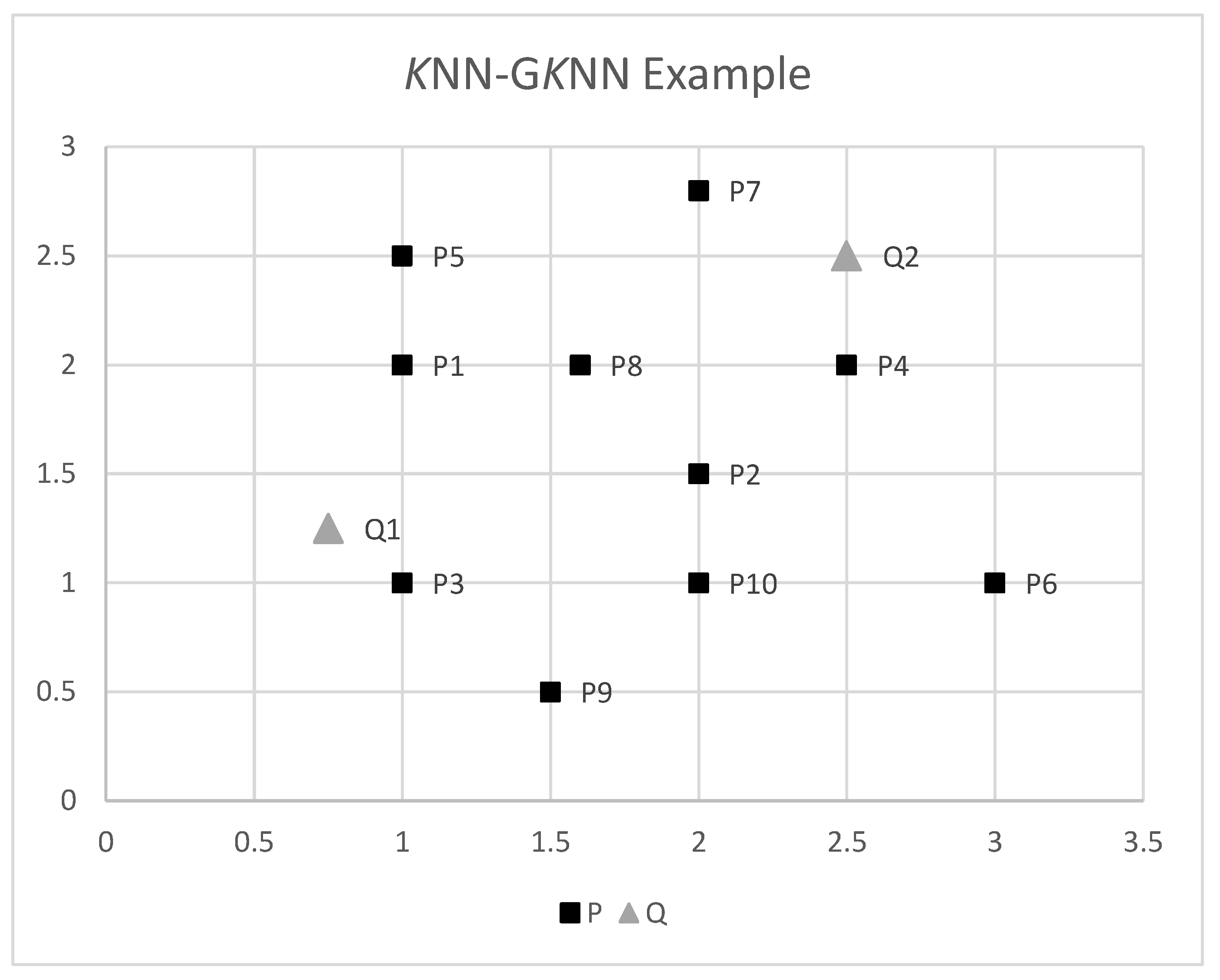
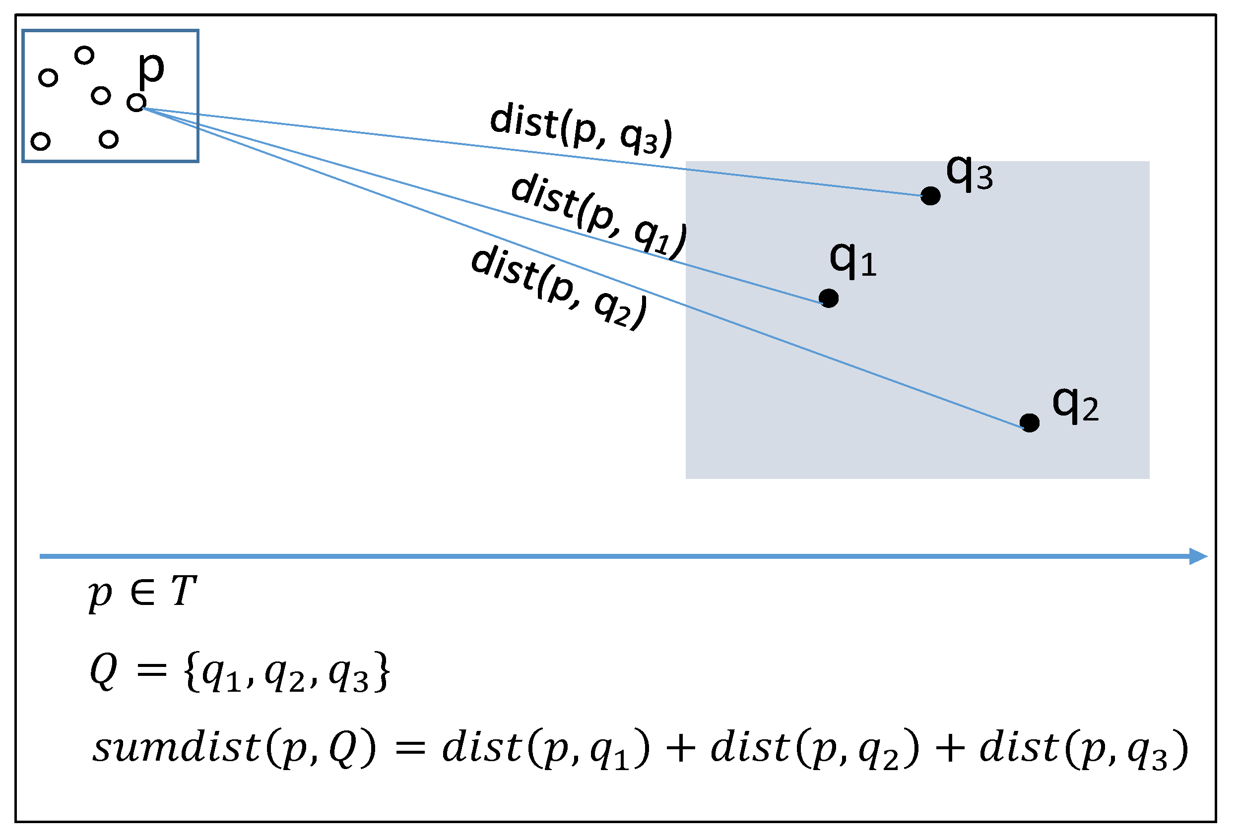
3.1. Group (K) Nearest-Neighbor (GKNN) Query

As it was introduced in [5], the GKNN query retrieves the K points from a set P (Training dataset) that has the smallest sum of distances from all points in another set Q (Query dataset).

GKNN query can be seen as an extension of the well-known and studied KNN query, where we search for the K closest points of a dataset to a given point.

Definition 1

(kNN). Given a point p, a dataset S and an integer K, the K nearest neighbors of p from S, denoted as $KNN(p,S)$, is a set of K points from S such that $\forall r\in kNN(p,S),\forall q\in S-kNN(p,S),dist(p,r)\le dist(p,q)$.

The distance function $dist$ is a distance metric defined on points in the data space. A very commonly used such distance function in spatial applications is the Euclidean distance, which is the one we will be using in this paper.

Definition 2

(GKNN). Given a dataset of points $P=\{P_1,P_2,P_3, \dots ,P_N\}$, a dataset of query points $Q=\{Q_1,Q_2, \dots ,Q_n\}$ and a number $K\in \mathbb{N},1\le K\le N$, the group K nearest-neighbor query is an ordered subset of P, denoted by $GNN(P,Q,K)$, where

$$GNN(P,Q,K)=\{p_1,p_2, \dots ,p_K:p_i\in P,p_i\ne p_j,1\le i,j\le K\}$$

and

$$\forall p\in P-GNN(P,Q,K):$$

$$\sum _{j=1}^{n}dist(p_1,Q_j)\le \sum _{j=1}^{n}dist(p_2,Q_j)\le \dots \le \sum _{j=1}^{n}dist(p_K,Q_j)\le \sum _{j=1}^{n}dist(p,Q_j)$$

So, the KNN query is a special case of the GKNN query, if the Query dataset only had one point. However, our algorithm incorporates several distinguishing characteristics that set it apart from other distributed KNN query solutions, such as sums of distances computations, with or without using the fast-sums technique, pruning heuristics for distant points and cells, cell-refining methods, and the mixing of local and distributed phases. These were thoroughly presented in [14] and are also briefly revised in Section 4.

In order to fully clarify the above definition, we present an easy to follow numerical example. For the sake of the example, consider the points in Figure 1. Suppose that we seek in P the 3 nearest neighbors ($K=3$) of the group of points Q, namely $GNN(P,Q,3)$. We also find the three nearest neighbors of every single Q point, namely KNN$(Q_1,P)$ and KNN$(Q_2,P)$. The (naive) approach for GKNN would be to calculate for each point in P the distances to every point in Q. Then, for each point in P, we find the sum of distances to all points in Q, then sort in increasing order, and select the 3 points of P with the smaller sum.

Table 3. Distance calculations.

	${\mathit{Q}}_1(0.75,1.25)$	${\mathit{Q}}_2(2.5,2.5)$	$\mathit{sumdist}({\mathit{Q}}_1,{\mathit{Q}}_2)$
$P_1(1,2)$	0.79	1.58	2.37
$P_2(2,1.5)$	1.27	1.12	2.39
$P_3(1,1)$	0.35	2.12	2.47
$P_4(2.5,2)$	1.9	0.5	2.4
$P_5(1,2.5)$	1.27	1.5	2.77
$P_6(3,1)$	2.26	1.58	3.84
$P_7(2,2.8)$	1.99	0.58	2.57
$P_8(1.6,2)$	1.13	1.03	2.16
$P_9(1.5,0.5)$	1.06	2.24	3.3
$P_{10}(2,1)$	1.27	1.58	2.85

shows their coordinates and the calculated distances, from which we easily deduce that KNN$(Q_1,P)=\{P_3,P_1,P_9\}$, KNN$(Q_2,P)=\{P_4,P_7,P_8\}$ and GKNN$(P,Q)=\{P_8,P_1,P_2\}$, ordered by ascending distance.

3.2. Apache Spark

Apache Spark [45] was first released in 2014 as an enhancement of Hadoop MapReduce [46,47,48]. Its later version is 3.1.2 and during these years of development it was proven to be much faster than Hadoop MapReduce in many cases [49,50,51]. Although the Spark machine aims to exploit the computing power of multi-core networked computers, recent efforts are underway toward integrating GPU acceleration within Spark.

Spark provides in-memory caching of data to a user application and allows the user to decide what data are cached and at what point of execution. By means of the in-memory caching, the disk I/O and network load are reduced, and data from intermediate computations are becoming directly available when needed. Spark offers APIs (with unequal maturity level) for writing code in R, Python, Scala and Java, but there exist several other interfaces for languages, such as JavaScript or C#. The most “natural” programming language to develop an application for Spark is Scala, but other JVM-based languages (and, of course, Java) may be used without serious performance overhead.

A Spark system consists of a driver running on a node designated as master of the cluster. Several executors are run within JVM instances on the slave nodes, communicate with the driver and perform the operations on data in parallel. In most cases, there is a single executor running per slave.

Spark is usually used in combination with a distributed file system, such as HDFS, where data are kept, and a cluster manager that coordinates the distribution of executors on the system, subject to the parameters set by the application. Its API relies on the abstraction of the resilient distributed dataset (RDD). Data are represented as RDDs in the Spark context, immutable collections of objects, and are distributed among slaves of the cluster. RDDs consist of logical partitions, regardless of the actual physical location of data (for example, in an HDFS file system) and Spark tries to allocate to each executor a task that requires data as close as possible to it in order to minimize network traffic. Several methods that operate on the RDDs and finally on the underlying data are provided. Additionally, Spark provides two kinds of shared variables: the broadcast variables that are written by the driver and read by the executors, and the accumulators that are written on the executors and read on the driver. By using a broadcast variable, one can broadcast a relatively small set of data from the driver to all executors, thus reducing traffic, and afterwards combine it with a larger dataset on them.

One significant characteristic of Apache Spark is that it exploits RDD dependencies and creates a directed acyclic /graph (DAG) of the execution plan, which allows executors to work in parallel on the data. To do so, Spark distinguishes two types of operations on the data: transformations and actions. The former returns a new RDD and is evaluated lazily, which means that it is not actually executed until an action is involved. A transformation may cause narrow or wide dependencies on the involved RDDs. In the case of narrow transformations, a single input partition creates a (modified) output partition, while in the case of wide transformations, data from more than one partitions need to be used/combined in order to create the child partitions of the new RDD. Typically, a wide transformation causes data shuffling, that is, network traffic.

Each time an action is invoked, the system inspects the lineage and creates an optimized execution plan, known as a job. Each job contains a number of stages, corresponding to wide transformations, and each stage consists of several tasks—one task per each partition of the output RDD, the actual parallel part of the execution, running locally on the executors.

Spark supports two built-in data partitioning schemes of RDDs on the nodes of the cluster. A hash partitioner spreads data across partitions by using a hash function on the key–value pairs of RDDs. A range partitioner assigns each partition data whose keys are in the same range. Since the default Spark partitioning techniques do not take into account the special characteristics of spatial data, it is obvious that they may not work well in spatial applications because, unless taken care of, Spark will distribute the data in a more or less random manner, ignoring the proximity among points. Therefore, implementing a proximity-aware partitioning of the data could significantly speed up performance because data points would be assigned to partitions depending on their spatial proximity [28]. In order to do so, one can either use a distributed spatial data management system built on top of Spark, as we will see in the next paragraph, or, if one wants to remain in plain Spark, then one must appropriately prepare the data and apply a custom partitioner.

4. GKNNQ Algorithm Essentials

While our algorithm for solving the GKNNQ in Spark is based on our MapReduce algorithm, as presented in [13,14], it is modified to exploit several Spark specific features, such as in-memory processing, functional programming and re-usability of local variables and RDDs.

4.1. MapReduce Algorithm Overview

The MapReduce algorithm consists of seven phases, four local and three distributed, with each local phase followed by a distributed one:

• Preliminary step. Local calculation of a sample-based quadtree, the sorted list of query points, query MBR and centroid coordinates, the sum of distances from centroid to Q. These are needed by most of the pruning heuristics.
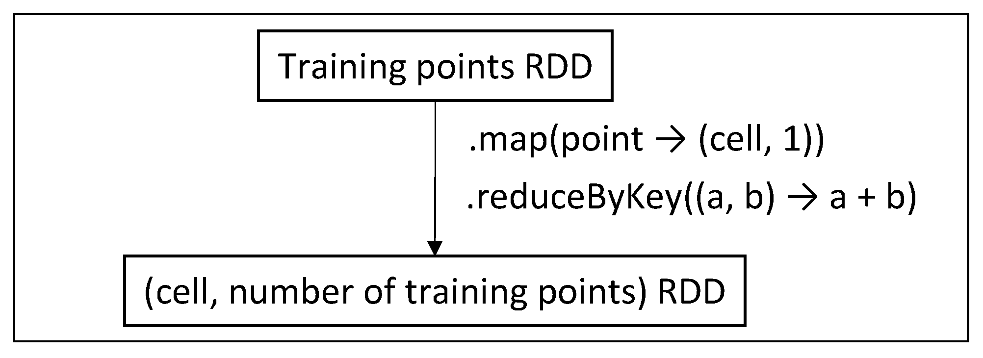
• Phase 1. Distributed computation of the number of training points per cell (needed by Phase 1.5).
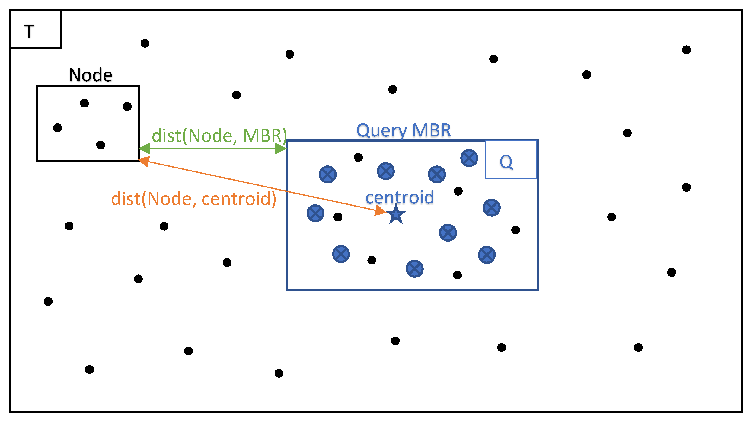
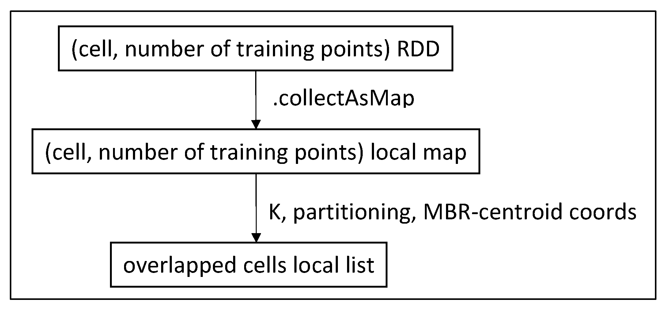
• Phase 1.5. Local discovery of a group of cells that contain at least K training points in total. Two methods are available so far: MBR and centroid circle overlapping. The second method is proved to be much more efficient because it includes fewer but generally better candidate points.
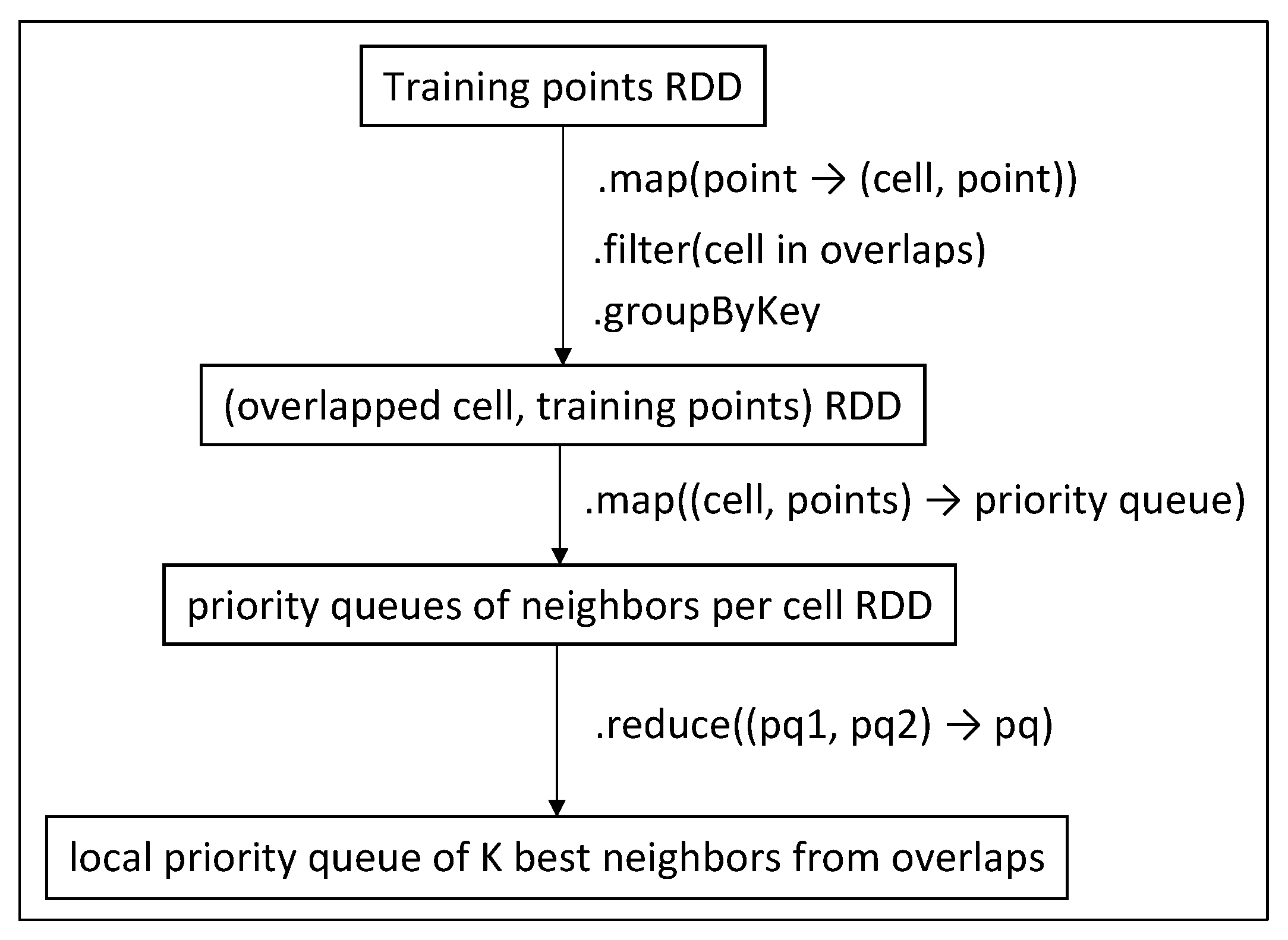
• Phase 2. Distributed computation of GKNN lists, one per intersected cell. Pruning heuristics are applied.
• Phase 2.5. Local merging of the GKNN lists into one with the best points found so far.
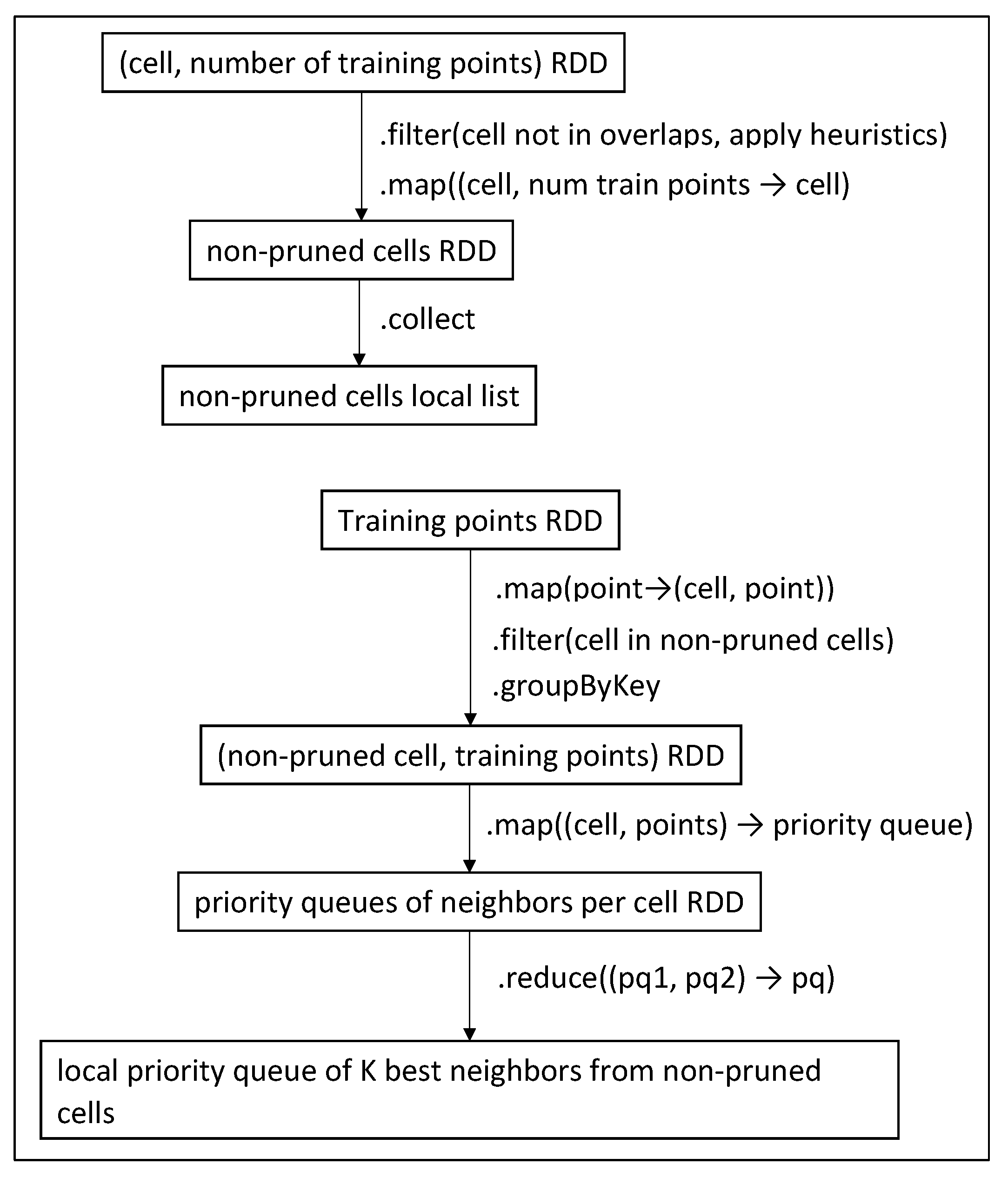
• Phase 3. Distributed computation of GKNN lists for the non-intersected cells. Heuristics are applied to prune distant cells to save unnecessary calculations. All new candidate neighbors are checked against the best ones from Phase 2.5.
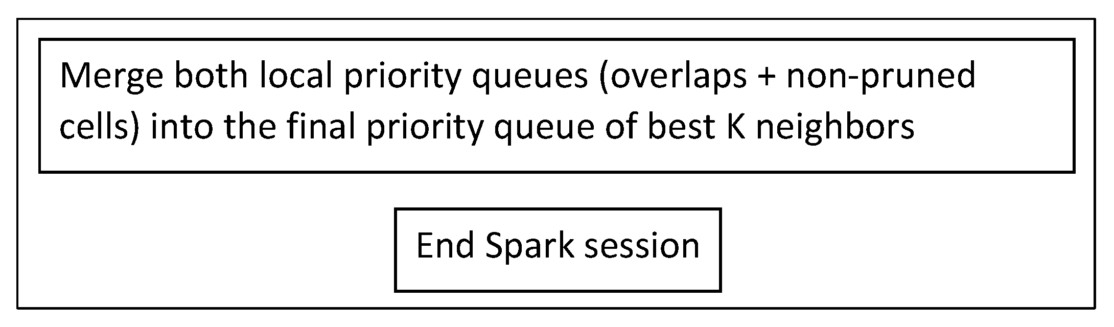
• Phase 3.5. Local phase (final) that merges the list of Phase 2.5 with lists from Phase 3 into the final one.

The experiments of [14] showed that between grid and quadtree partitioning, brute-force and plane-sweep reducers and MBR and centroid circle overlaps, the best performing combination is grid with brute-force using centroid cell overlaps, so this is the combination we use in this paper. We now briefly present these methods.

4.2. MBR and Centroid Circle Selection Methods

In local Phase 1.5, we seek a first estimation of the final GKNN query, that would be as close as possible to optimal. This may be achieved by discovering a (small as possible) “target” group of cells that are more likely to obtain this good estimation. Needless to say, these cells must contain at least K training points in total. In Phase 1, we have counted the points within each cell, so we can use this result.

In the MBR selection method, all cells that intersect with the query MBR are eligible for searching for candidate neighbors. The problem is that there are too many points to examine, and Phase 2 has an excessive amount of work to do. In the centroid circle method, the eligible cells are significantly reduced so that only those who intersect with a generally small circle around the centroid (expanded if necessary to include at least K training points) are checked for neighbors. Both methods are shown in Figure 2 and Figure 3. See [14] for the pseudo-codes.

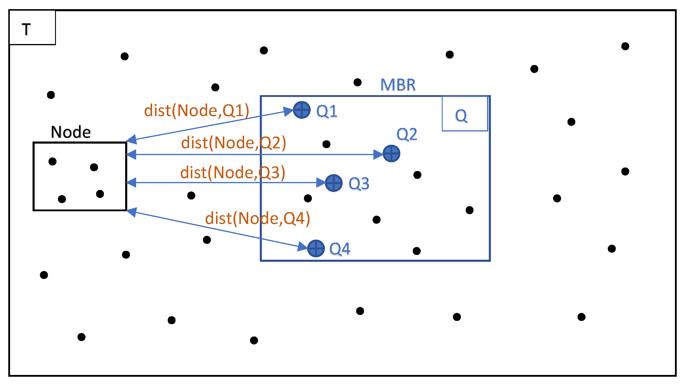
4.3. Pruning Heuristics

In Figure 4 we can see the query dataset’s MBR and centroid, surrounded by the Training dataset and an arbitrary node (cell), created by partitioning.

The centroid, which we use quite frequently, is a point in space that has the minimum sum of distances to all query points. If it coincides with a Training point, it would make it the ideal nearest neighbor for this query. However, it generally is an imaginary point, and its coordinates are calculated numerically in the preliminary phase of the algorithm (see [5,14]).

Table 4. Symbols.

Symbol	Description
$\left|Q\right|$	cardinality of Q
$sumdist(p,Q)$	sum of distances from point p to all points of Q
$best\_dist$	K-th nearest-neighbor distance
$dist(Node,p)$	min distance between $Node$ and point p
$dist(Node,MBR)$	min distance between $Node$ and Query $MBR$

contains the symbols used to describe the pruning heuristics that help us prune lots of non-eligible Training points and cells.

• Heuristic 1: $Node$ can be pruned if:

  $$dist(Node,centroid)\ge \frac{best\_dist+sumdist(centroid,Q)}{\left|Q\right|}$$
• Heuristic 2: $Node$ cannot contain qualified points if:

  $$dist(Node,MBR)\ge \frac{best\_dist}{\left|Q\right|}$$
• Heuristic 3: $Node$ can be pruned if:

  $$\sum _{q\in Q}dist(Node,q)\ge best\_dist$$
• Heuristic 4: Training point p can be pruned if:

  $$dist(p,centroid)\ge \frac{best\_dist+sumdist(centroid,Q)}{\left|Q\right|}$$

Heuristics 1, 2 and 4 are visualized for better understanding, in Figure 5. The geometric data are taken from datasets used in experiments and depicted in Figure 6.

The circle has its center on the query centroid, and its radius is calculated from the right member of the Heuristic 1 inequality. The rounded rectangle’s perimeter has a distance from the query MBR equal to the right member of the Heuristic 2 inequality.

Any cell from any partitioning method that intersects with the circle will not be pruned by Heuristic 1. Any cell from any partition method that intersects with the rounded rectangle will not be pruned by Heuristic 2. All cells outside these two shapes are automatically pruned. The circle also works for Heuristic 4; every single training point outside the circle is pruned. The cells that pass Heuristics 1 and 2 will be checked by Heuristic 3, which is more costly (Figure 7); those cells which will not be pruned at all and will be checked for neighbors inside Phase 3.

Figure 7 shows a visualization of Heuristic 3. The node depicted either intersects the circle or the rounded rectangle of Figure 5 or is located inside them; in any case, it was not pruned by Heuristics 1 and 2. If $Q=\{Q1,Q2,Q3,Q4\}$, then the left member of the Heuristic 3 inequality takes the form

$$dist(Node,Q1)+dist(Node,Q2)+dist(Node,Q3)+dist(Node,Q4)$$

In simple words, if the node’s sum of distances to all query points is bigger than the K-th nearest-neighbor’s distance, then any of its points will have an ever bigger sum of distances and thus, will not qualify as the better nearest neighbors. The gain is that we have to calculate only |Q| distances, instead of

$$\left(numberoftrainingpointsinsideNode\right)\times \left|Q\right|$$

Heuristics 1, 2 and 3 are found in the first filter function of Figure 8, while Heuristic 4 is applied in Figure 8 and Figure 9 when we map the points to a priority queue (inside the brute-force algorithm).

4.4. Grid Partitioning

Only grid partitioning is used in this paper. In grid partitioning, the space is divided into $N\times N$ equal square cells. N is a user-defined parameter, and it plays a major role in the algorithm’s performance. When changing N, we modify each cell’s size (bigger N means more, smaller cells, smaller N means fewer, bigger cells) and thus, its ability to contain more or less points. When a cell contains many points, the number of calculations inside it grows quadratically. Few but big cells will give the executors a lot of calculations to perform. Many but small cells will result in faster computations, but will generate many executor processes, which is also undesired.

The grid’s advantage is fast point and cell location. If we know N, we are just a few easy algebraic calculations away from knowing where each cell and point is located. Its disadvantage is that we cannot control the number of points inside each cell; it just applies blind cuts. Some cells may have few or no points, while others may have thousands or more.

4.5. Brute-Force Computation Method

In [14], we used two computational methods: brute-force and plane-sweep. Plane-sweep is more sophisticated, but also more complicated, and it loses to naive brute-force because of the heuristics described in Section 4.3 that practically overcomes plane-sweep’s superior pruning capabilities. Brute-force in GKNNQ works as shown in Figure 10.

Imagine a single cell containing several training points, from which we want to find the best K ones. We start calculating the sum of distances from every training point to all query points. The first K points are inserted into a max heap, along with their sum of distances. We continue to check every other training point in the cell; and if we find a smaller sum of distances, we replace the top of the heap with this point, and so on. Only Heuristic 4 (Section 4.3) is applied here. The brute-force pseudo-code is presented in [14].

In [14], we also introduced a technique, called “Fast Sums”, to avoid performing repetitive sums of distances computations in pruning heuristics and also when checking each individual candidate neighbor. In Heuristic 3, when we calculate the left member of the inequality, if and when the sum becomes bigger than the K-th neighbor’s distance, the calculation stops and the function returns. The same thing happens when we check the sum of distances of a candidate neighbor against the K-th neighbor’s distance in the priority queue in the brute-force method. The experiments showed that it can indeed save many needless calculations. Thus, we have it turned on by default.

4.6. Usage of Techniques per Phase

In our previous works we have presented two partitioning methods (grid and quadtree), two cell selection methods (MBR and centroid circle) and two computation methods (brute-force and plane-sweep). Out of these eight possible combinations, our experiments showed that the best performing one is grid partitioning with centroid circle selection and brute-force computation, which we use in this paper.

Partitioning is used in distributed phases 1, 2 and 3, to map the training points to their cells. Centroid circle selection method is only used in local Phase 1.5. Brute-force computation is used in distributed Phases 2 and 3 to find the candidate neighbors out of the selected training points.

5. A Spark-Based GKNN Query Processing Algorithm

Utilizing the ideas and techniques from Section 4, we now present the Spark-based algorithm. The presentation compares each phase and step to the MapReduce version in order to manifest the differences and similarities in implementation.

5.1. Preliminary Phase

In the Spark approach, only the preliminary phase runs separately (Figure 11), while all the others are unified and run inside the main function.

On the other hand, in MapReduce, the preliminary phase and also every other phase runs separately.

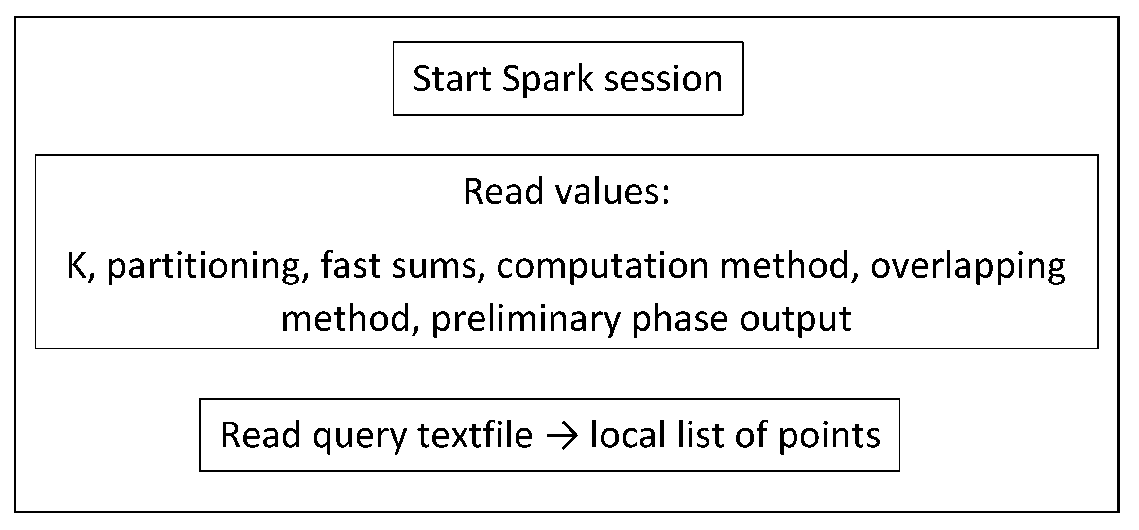
5.2. Starting Spark Session

First (Figure 12), we read the required values and the query dataset file into a local list of point objects $(id,x,y)$. The query dataset is considered small enough to fit into a local list. Then (Figure 13), we read the training dataset file into an RDD of point objects.

In Spark, these values are read only once and stored into local variables, and then are passed as parameters in functions. In MapReduce, these values are read/written from/to HDFS or given as user parameters every time they are needed in each phase. The process of Figure 13 does not occur at all; instead, the training dataset file is read again and again each time it is needed.

5.3. Computing the Number of Training Points per Cell (Phase 1)

We now need to create a “density map” which will provide us with the information of the number of training points per cell (Figure 14). Mapping a point to its cell requires information from partitioning.

In MapReduce, we employ a Mapper and a Reducer separately to implement the corresponding functions. The training points dataset is read from HDFS, while in Spark, we transform the previously prepared training points RDD into a new one, using concise functional programming code.

5.4. Searching for Overlapped Cells (Phase 1.5)

Then we run a function similar to local Phase 1.5 to discover the cells that overlap with a circle around centroid and contain at least K training points in total. This function runs on the driver only. Partitioning gives us the information of where the cells are located, and the locally collected RDD from Phase 1 tells us how many training points each one contains. The procedure is depicted in Figure 15.

This process in MapReduce is almost identical, except for the obvious difference of the input being read from HDFS files and the output being written in HDFS as well, instead of already prepared RDDs and local data structures.

5.5. Creating a First Approach of the Neighbors List (Phases 2 and 2.5)

Afterwards, we use the training points inside the overlapped cells to create an intermediate RDD of (cell, training points in this cell) tuples, using the $groupByKey$ function, on which we apply the appropriate calculation method, using the $map$ function to create a priority queue of the best K neighbors per cell. These priority queues are finally merged into a single one, using a proper $reduce$ function, and it is locally stored on the driver. The procedure is depicted in Figure 9.

Each priority queue contains the (training point id, sum of distances from all query points) tuples, ordered by the sum of distances. The second $map$ function uses the selected calculation method (brute-force in this case) to discover the best neighbors from each cell and insert them into a priority queue.

In MapReduce, the Mapper reads again the training dataset from HDFS and converts it to point objects, giving the intermediate output <$overlappedcell,trainingpoints$>, which is written to HDFS. The Reducer reads the output, converts the string values to cell and point objects, and passes them to the function that discovers the K nearest neighbors in each cell. The result is written to HDFS as text files containing the id’s and distances of the neighbors. Then, the local Phase 2.5 reads all these text files, converts the string values to objects and inserts them into a single priority queue. In Spark, we use transformations on previously prepared RDDs, without reading and converting any text files. Local Phase 2.5 is incorporated here as the $reduce$ command, which also acts on an RDD.

5.6. Searching for Neighbors in Distant Cells (Phase 3)

Now that we have created a preliminary list of neighbors from the overlaps, we must also check the rest of the cells. The sum of distances of the K-th neighbor, which was found in the previous phase, is used in the pruning heuristics (Section 4.3). We use the cell-training points RDD from Phase 1 (Figure 14), keeping the cells only and excluding the overlapped cells; then, we apply cell pruning heuristics. If any cells pass through, they are collected into a local list. The procedure is displayed in the upper half of Figure 8. Phase 3 neighbors are derived from the training points RDD, using a series of transformations, similar to Figure 9, and are presented in the lower half of Figure 8.

In MapReduce we employ two Mappers; the first one reads the output of phase 1 from HDFS and applies heuristics to prune cells, while the second one reads again the Training dataset file from HDFS and performs point location giving the output <$cell,trainingpointidandcoordinates$>. Both Mappers’ outputs are then grouped by cell and fed to the Reducer. The Reducer merges both Mappers’ outputs and passes the eligible training points to the function that discovers the K nearest neighbors in each cell. Another difference between Spark and the MapReduce version is that MapReduce’s Reducer creates multiple priority queues (one per cell) as text files in the end of Phase 3, while Spark merges them into a single one, using the $reduce$ function of Figure 8.

5.7. Creating the Final List of K Neighbors (Phase 3.5)

MapReduce’s local Phase 3.5 is now a merging of the priority queues of Figure 8 and Figure 9 on the driver, which produces the final neighbors list, as shown in Figure 16. The Spark session ends here.

In MapReduce, a local function reads the text files from HDFS that contain the multiple neighbor lists of Phase 3 and the single one from Phase 2.5 and merges them to the final one, after performing the necessary conversions from strings to doubles. In Spark, there are only two lists of neighbors as objects (one from Phase 2 and one from Phase 3) already loaded in RAM.

5.8. Review of the Similarities and Differences in Spark and MapReduce Implementation

It should be obvious at this point that the original MapReduce GKNN query algorithm has undergone several improvements in its Spark implementation.

MapReduce’s programming model demands reading and writing text files only in the form of <$key,value$> to and from the distributed file system. In a multi-phase algorithm, such as this one, this happens in every phase; the same big files have to be re-read several times, and their string values are converted to other structures and vice versa.

In Spark, we have to read each big file only once and then, applying suitable transformations, convert it to an RDD of objects, which can be loaded in distributed memory once and used many times afterwards. We did this with the training points and the query points datasets and also with the intermediate results that derived from transformation on the aforementioned RDDs. We also merged together Phases 2 and 2.5 and reduced the output size of Phase 3. In addition, by persisting some RDDs, the disk I/O was kept at a bare minimum. Spark’s functional programming model allowed us to simplify the whole process and reach the same results per phase in a more concise way.

There are, however, some functions and classes from the MapReduce version, which were transferred to the Spark version with minimal changes, such as the local phases, the partitioning, the pruning heuristics and other minor computational functions.

6. Improvements on the Spark-Based GKNN Query Processing Algorithm

The previously presented algorithm proved to be quite efficient, compared to Hadoop, but there are still a couple of improvements that may further boost its performance. We make use of two facilitations of the Spark framework, which are broadcasting local variables and persisting RDDs into memory or disk for repeated usage.

Firstly, we broadcast the local list of query points (Figure 12) to all workers as soon as it is created. This list is available locally to all workers, instead of being transmitted every time it is needed for calculations, which is for every mapping of $(cell,points)$ tuple to a priority queue in Phases 2 and 3 (Figure 8 and Figure 9). Depending on the query dataset size and the network speed, this could significantly decrease the overall time.

Secondly, we persist the most frequently used RDDs, which are the training points RDD, created right after starting the Spark session (Figure 13) and used in Phases 1, 2 and 3 (Figure 8, Figure 9 and Figure 14) and the $(cell,numberoftrainingpoints)$ RDD, created in Phase 1 (Figure 14), used in Phases 1.5 and 3 (Figure 8 and Figure 15).

The efficiency of both these improvements are tested in the experiments.

Spark DAG

A deeper look on the algorithm from Spark’s point of view and also a proof of the effectiveness of persisting the training points RDD comes from the Spark DAG.

We know that Spark’s web UI displays the DAG for each job, where vertices represent the RDDs and edges represent the transformations applied on them. We show one part of the DAG created for this algorithm and analyze it.

In Figure 17, we can see the DAG generated by the $reduce$ action of Figure 8, where the local list of neighbors from distant cells is formed. Stage 20 reads the training dataset text file from HDFS (box A) and transforms it into an RDD of point objects (box B), as shown in Figure 13. Then, it maps each point to a $(cell,point)$ tuple (box C) and filters out the pruned cells (box D), as shown in the lower half of Figure 8. All these commands belong to the same stage because they are narrow transformations and they do not require shuffling of data. Stage 20 is marked as “skipped” because we have persisted the training points RDD, so the transformations of boxes C and D are applied on the previously computed (in an earlier step) and cached RDD of box B.

However, when the wide transformation $groupByKey$ (box E) is applied, data are shuffled and a new stage is created (21). $mapValues$ of box F typically follows $groupByKey$, while $mapValues$ of box G is the transformation of points into a priority queue of neighbors, as seen in the last map function of Figure 8. The $map$ function in box H stands for the $values$ command, which is not displayed in Figure 8 for simplicity, and is used in order to remove the cells inside the $(cell,priorityqueue)$ tuples. The $reduce$ action is then executed.

7. Experimental Results

The Spark algorithm, as presented in Section 5, is thoroughly tested against its Hadoop counterpart (from [14]), using a variety of dataset combinations. A per phase direct comparison is also included. Furthermore, it is tested for scaling as K grows larger and computing nodes become fewer. Finally, we present experiments testing the improvements discussed in Section 6.

7.1. Datasets and Test System Configuration

We use three real-world datasets as training and one real and two clustered synthetic ones as query. The training datasets contain the coordinates of parks, buildings and road networks around the world from OpenStreetMap (http://spatialhadoop.cs.umn.edu/datasets.html, accessed on 16 August 2021) [3] and have 11.5M, 114.7M and 717M points, respectively. The real query is based on one that contains linear hydrography coordinates inside the U.S.A., but we have trimmed the farthest points and halved it, so it now contains 2.8 million points. The synthetic query datasets originally contain 10M and 50M points, scattered in concentrated regions all around the globe. We have cropped them to a rectangle that roughly covers the African continent and they now contain fewer points. All datasets’ coordinates are normalized in the $[0,1]$ range, in order to simplify the algorithms. We also performed experiments with one query dataset moved to other locations, for performance comparisons. Figure 6 shows the smaller clustered synthetic query and the road networks training datasets. Figure 18 shows the default and new hydrography query dataset locations over the road networks training dataset. Figure 19 shows the larger clustered synthetic query and the parks training datasets.

Table 5. Datasets.

Type	Dataset	Num. of Pts	Disk Size
Training	parks	11.5 million	373 MB
	buildings	114.7 million	3.7 GB
	roads	717 million	30 GB
Query	hydro (def. loc.)	2.8 million	91.4 MB
	hydro (new. loc.)	2.8 million	91.4 MB
	small synth.	706,000	29.5 MB
	large synth.	39 million	165.7 MB

shows some properties of the datasets used.

We have set up a cluster of nine virtual machines (one Namenode/Driver and eight Datanodes/Workers) running Ubuntu Linux 20.04 64-bit. Each machine is equipped with a Xeon quad core at 2.1 GHz and 16 GB RAM, connected to a 10 Gbit/sec network. Hadoop experiments are run on version 3.2.2, while Spark experiments are run on version 3.1.2. Each virtual machine corresponds to a single Hadoop Datanode/Spark Worker and each Worker runs one Executor process, which means that there are eight Workers/Executors in the cluster, plus the driver. Each Executor has 4 cores and 12 GB of memory allocated.

Grid partitioning is used, the cell overlapping method is the centroid circle, and neighbors discovery is performed using the brute-force approach. The fast sums method is used for pruning distance sums computations. The grid space decomposition parameter is N, which means that the training dataset is divided in $N\times N$ square cells. The broadcasting of local variables and persisting of RDDs is used, as analyzed in Section 5, unless otherwise stated. The value of K is 10 and the number of computing nodes is 8, except for the scaling experiments.

Each experiment was executed three times, and the running time was averaged. We ran the preliminary phases separately and did not include them into the performance graphs. Using these particular query datasets (on which ones the preliminary phase runs exclusively), their running time was less than a minute. So, the total running time of each experiment was from the start of the Spark session to its end (Figure 12, Figure 13, Figure 14, Figure 15 and Figure 16).

We present the graphs of the experiments in this section and discuss the results in Section 8.

7.2. Hadoop vs. Spark Experiments

In Figure 20, Figure 21 and Figure 22, we can see Spark’s performance as a function of N and compared to Hadoop. The datasets are the small synthetic queries versus the three training ones, ordered by cardinality.

The range of values of N in each graph are derived from experiments to determine the optimal N, and then we present the algorithm’s performance near it.

In Figure 23, Figure 24 and Figure 25 the small synthetic query is replaced by the large one.

Finally, Figure 26 and Figure 27 show how the real query dataset, in both default and new locations, behaves against the large training.

Figure 28 shows the absolute and relative performance differences per distributed phase and in total for a certain dataset combination.

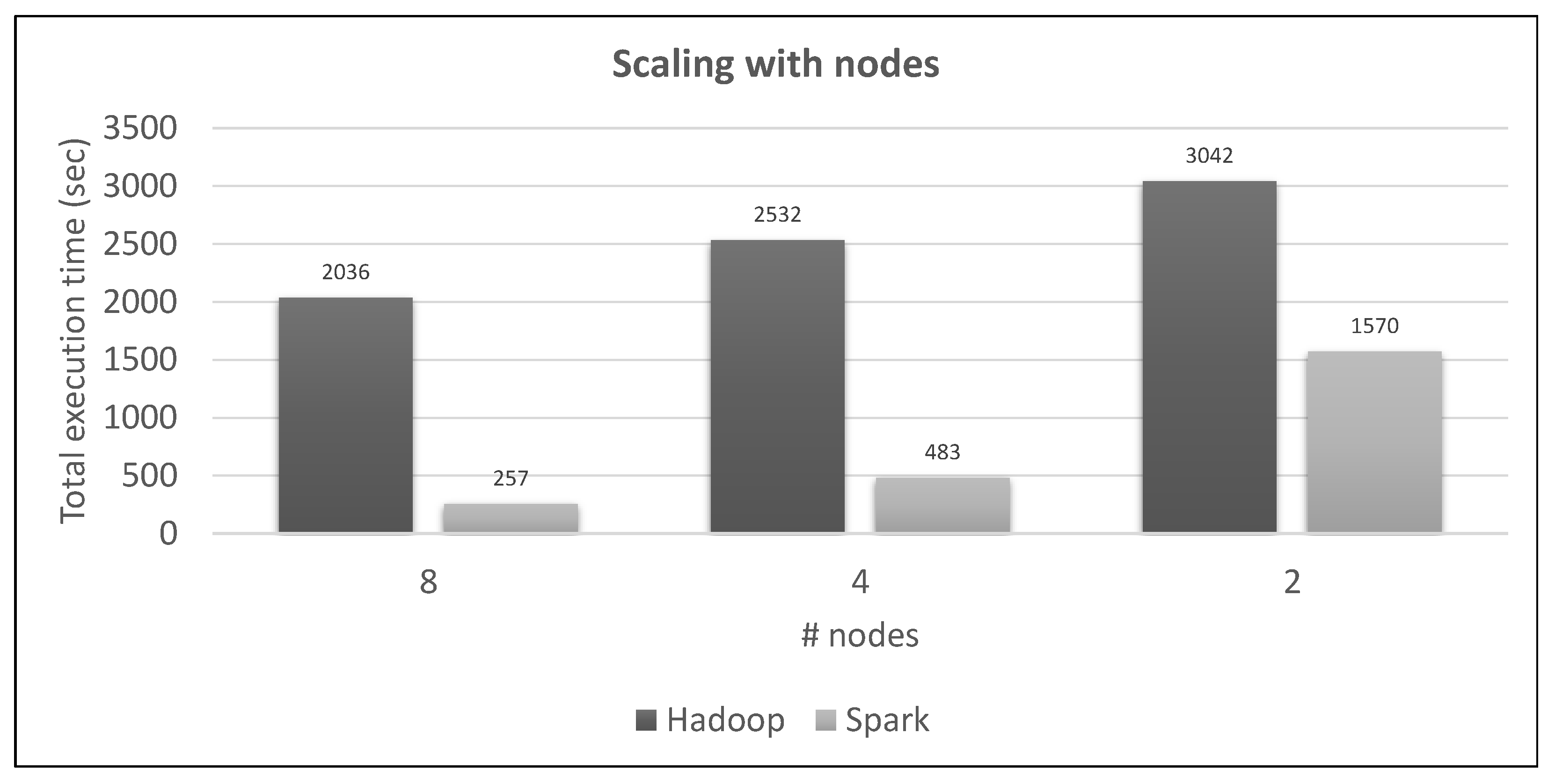
7.3. Scaling Experiments

In this section, we will test Spark’s capability of scaling with K and the number of available workers. The datasets used are small synthetic query vs. medium training (Figure 21), using the best performing N = 3600.

In Figure 29, we see how the algorithm scales on Spark with much bigger values of K.

In Figure 30, we see both frameworks running a specific combination of datasets with some computing nodes decommissioned.

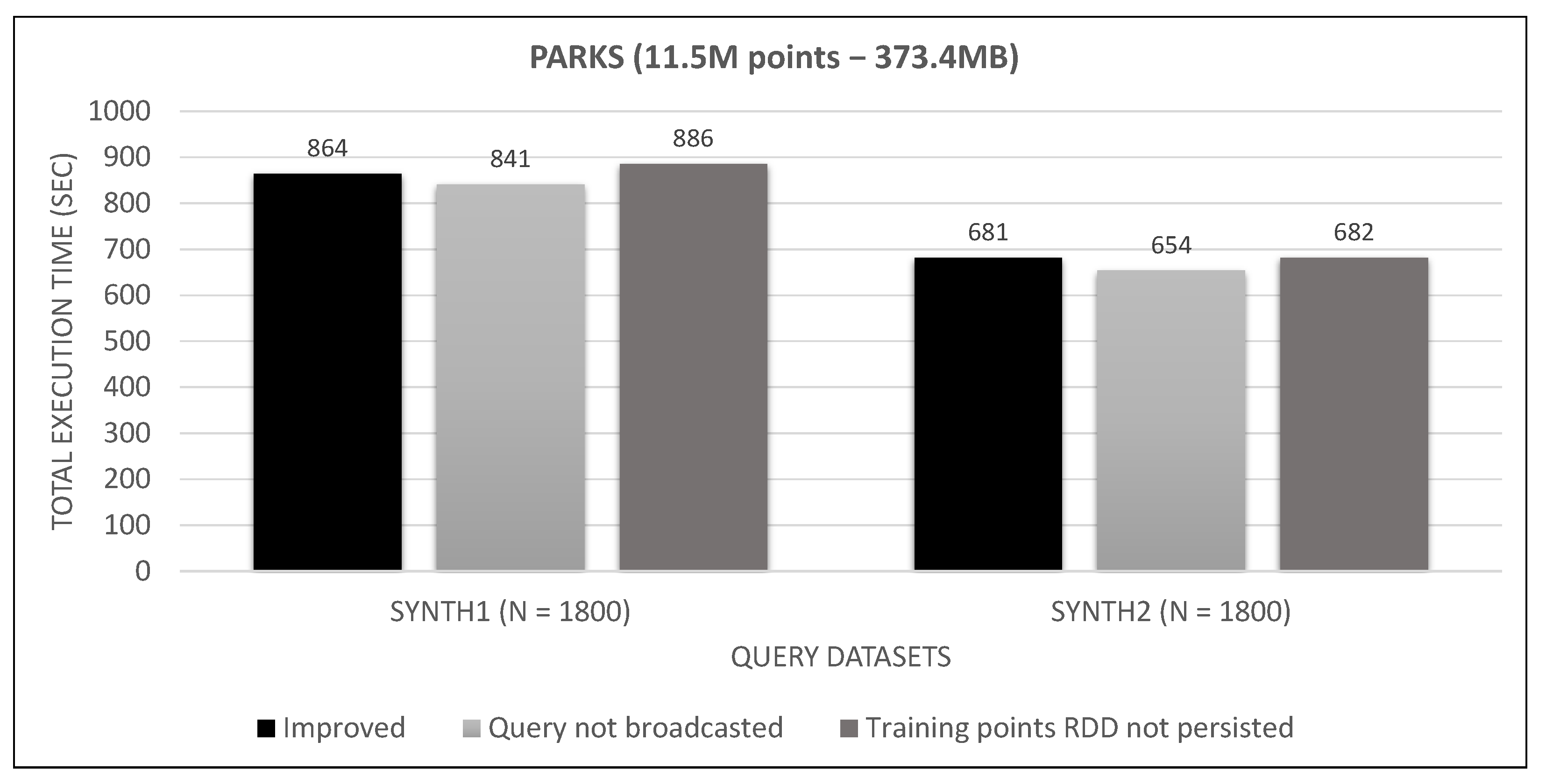
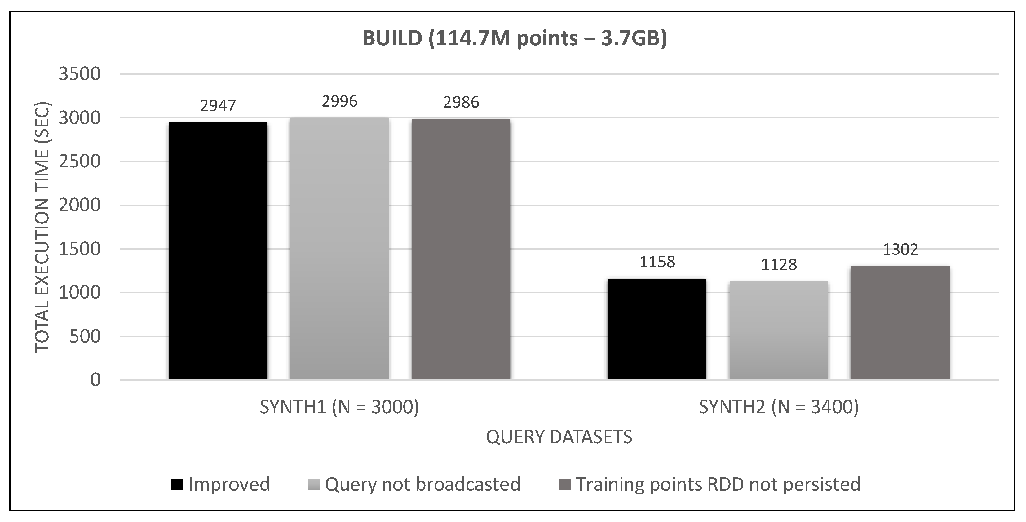
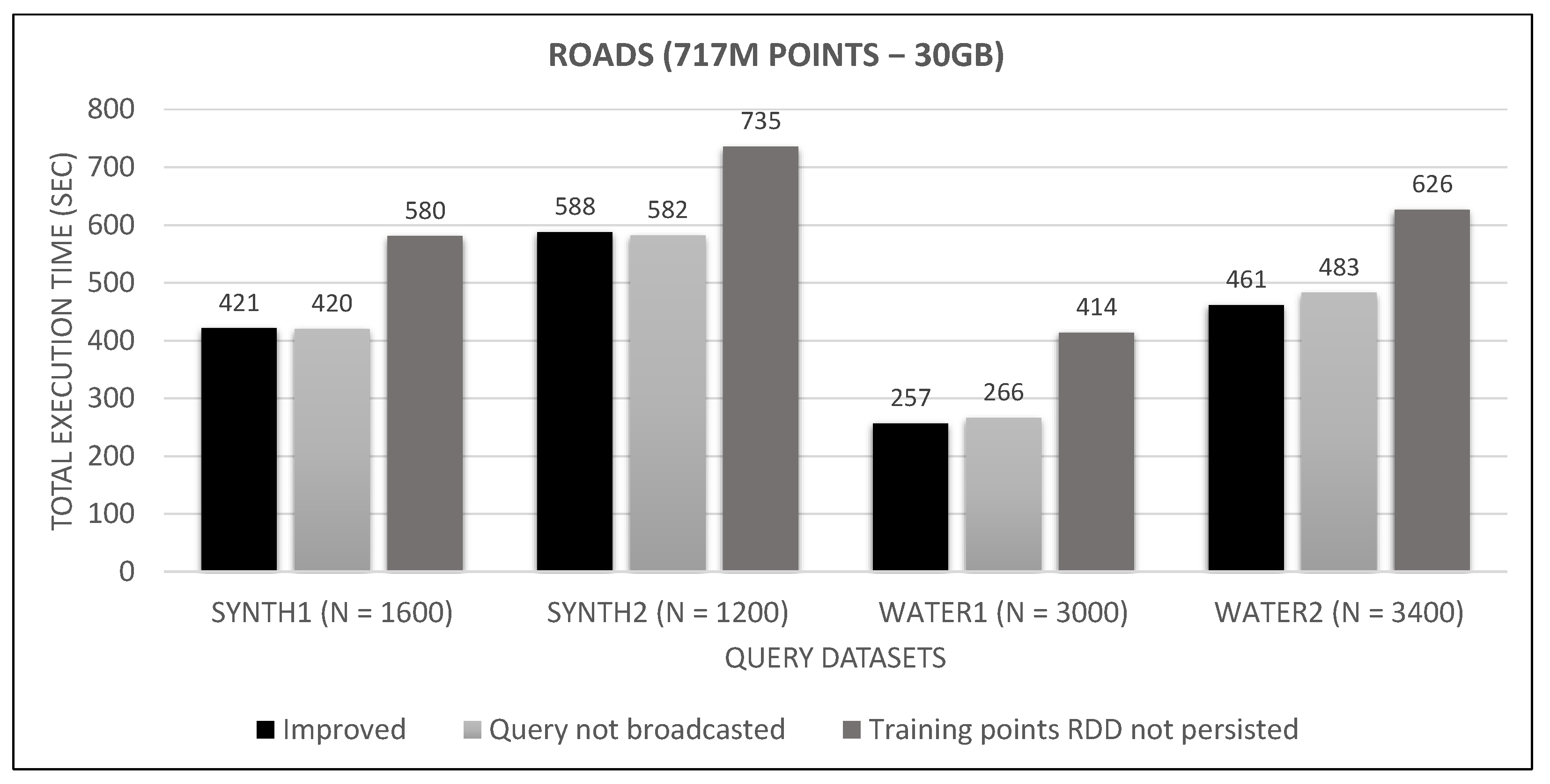
7.4. Spark Algorithm, Improved vs. Base

We now test the improved algorithm (the one used so far in the experiments) against the base one, which has some features turned off. One such feature is the broadcasting of the query dataset, and another is the persisting of the training points RDD, as described in Section 5.

Firstly, we deactivate the broadcasting of the query dataset (Figure 12) so that every time it is needed, it is transmitted to all workers. This will happen for every cell examined by Phases 2 and 3. Secondly, we try not persisting the training points RDD (Figure 13) to see if its re-computation will gain an advantage over the cached one’s serialization/de-serialization CPU overhead. The results are depicted in Figure 31, Figure 32 and Figure 33.

8. Discussion

Having presented all the graphs from the experiments, we can now discuss and interpret them. First of all, it must be noted that space partitioning is exactly the same for both systems; utility classes and functions are mostly unchanged; pruning heuristics and fast sums technique are applied similarly; and each phase processes the same points for each dataset couple and N. Consequently, Spark’s superior performance derives primarily from its in-memory handling of data and the algorithmic and coding adaptations performed toward that direction, instead of Hadoop’s constant read/write to disk.

Looking at graphs in Figure 20, Figure 21, Figure 22, Figure 23, Figure 24, Figure 25, Figure 26, Figure 27 and Figure 28, we observe the following:

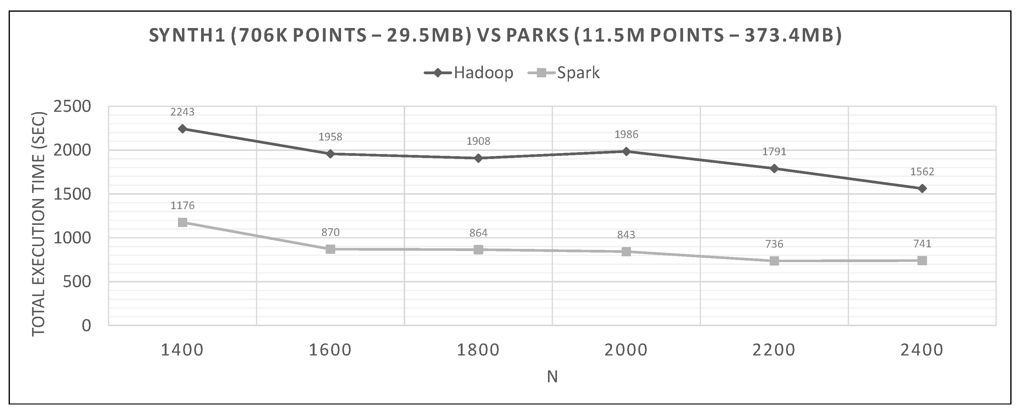
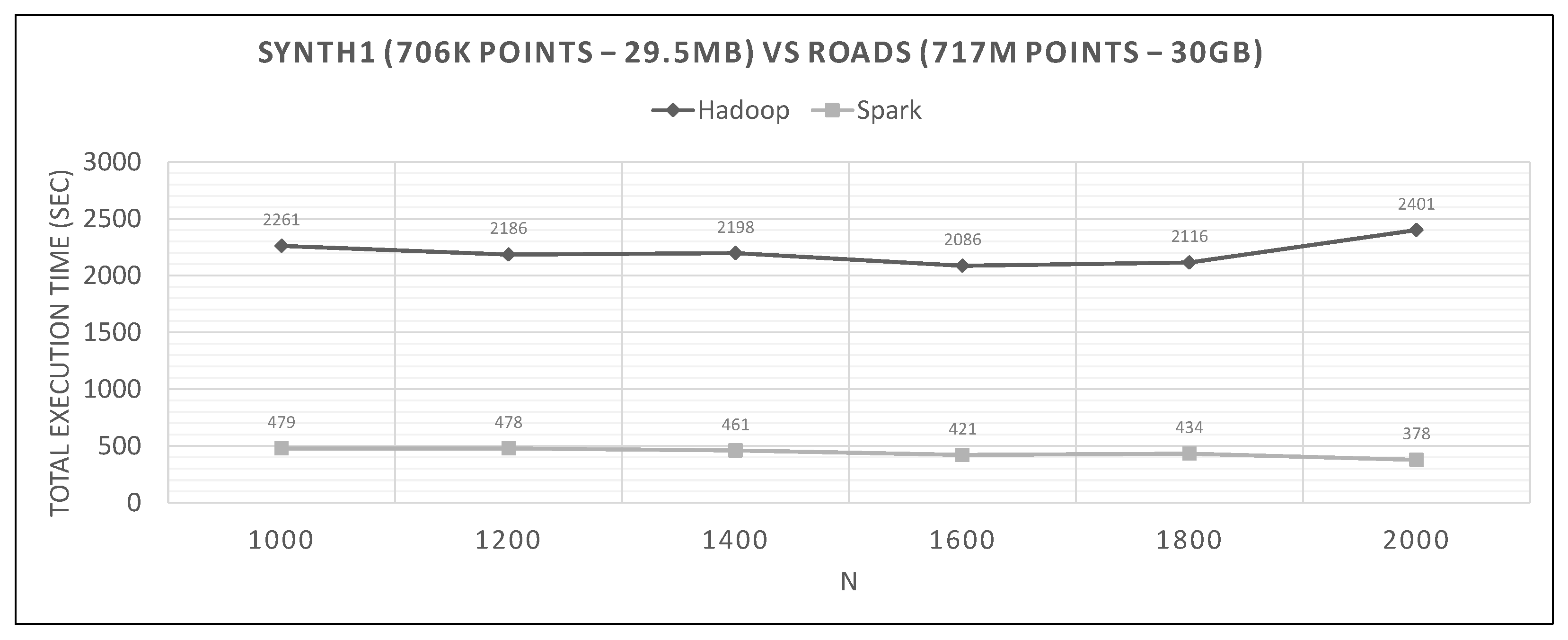
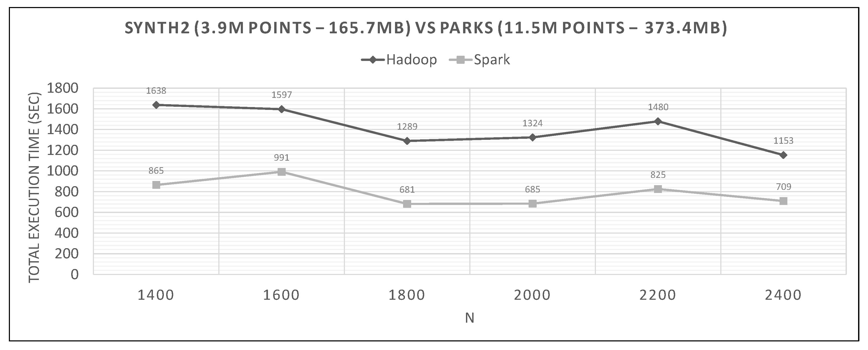
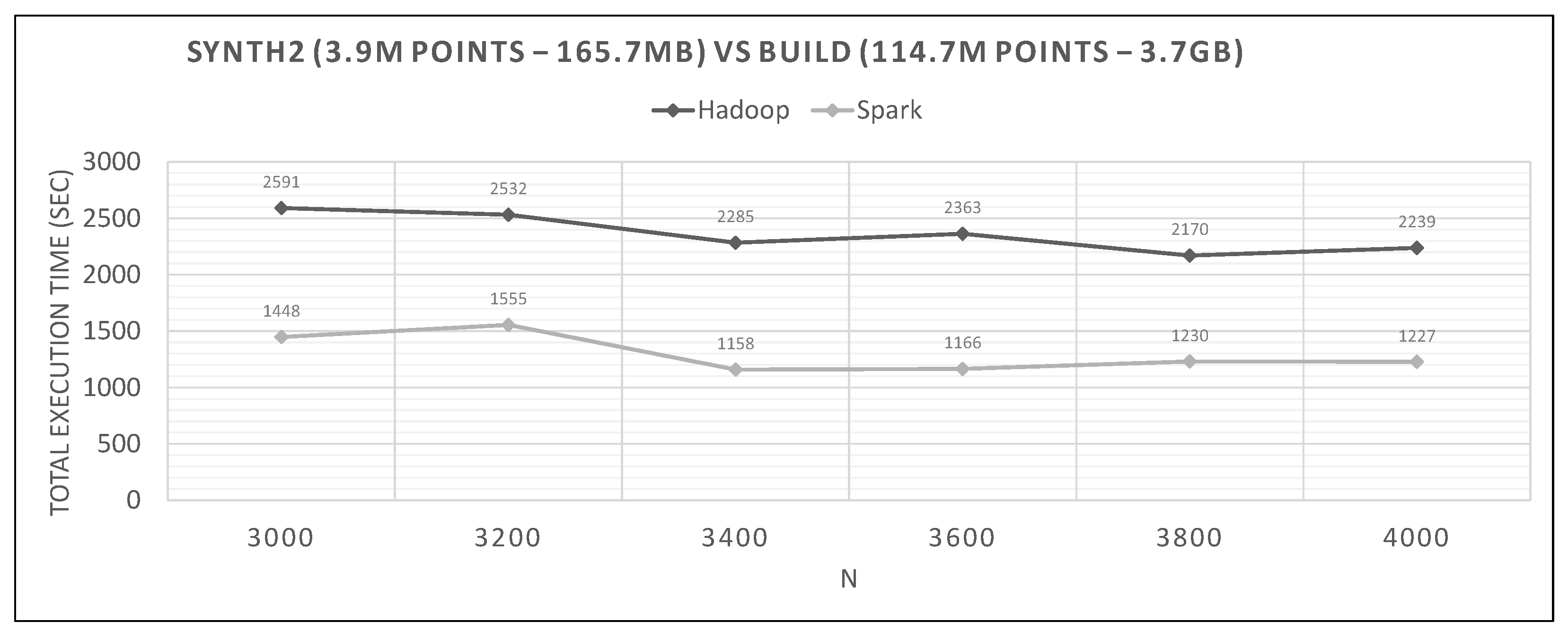
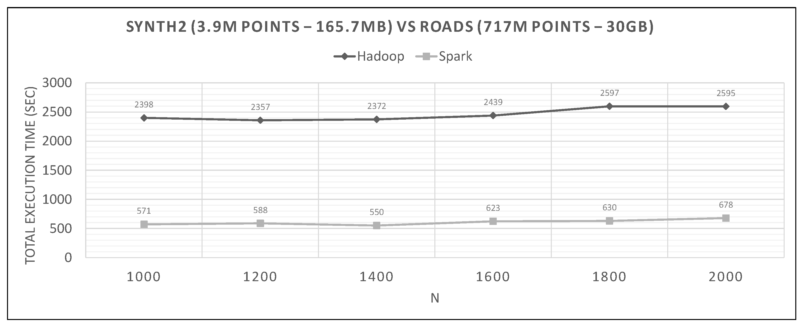
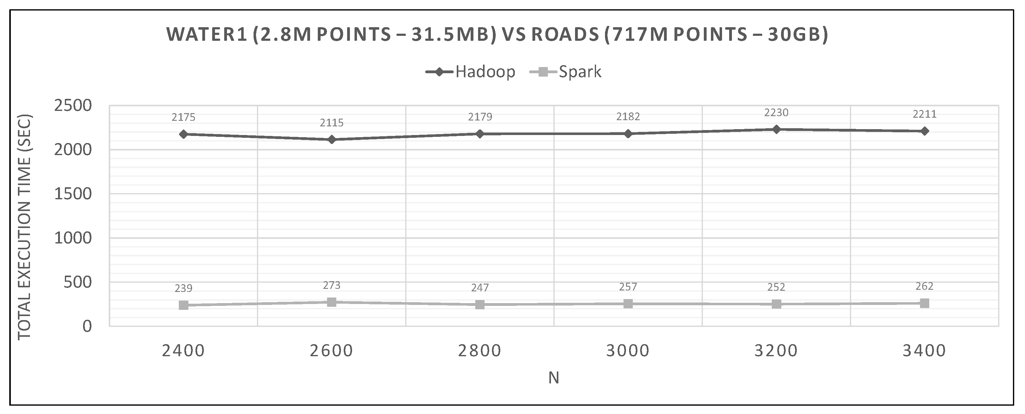
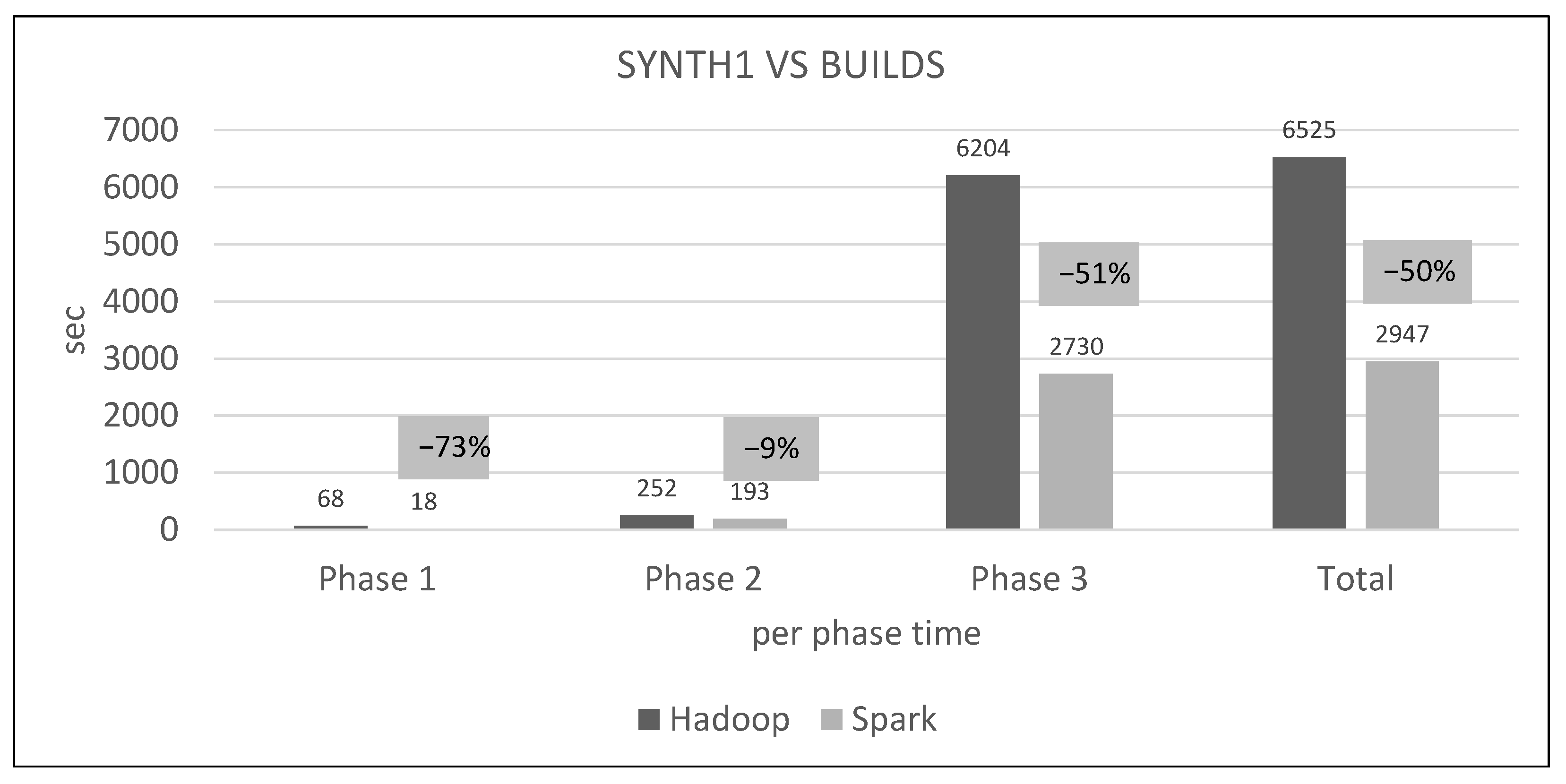
• Spark finishes 50–90% faster than Hadoop. Similar percentages apply to each distributed phase of the algorithm.
• Spark’s performance remains mostly unchanged for a wide variation of N; it is an almost flat line in many graphs. However, the best performing Ns are the larger ones, as can also be observed for Hadoop in these experiments and in the literature (Section 2.2). More cells mean fewer points inside each and, therefore, fewer calculations per cell.
• The optimal value of N varies significantly for each dataset couple, and it is hard if not impossible to foresee it without experimentation, mostly because of the unpredictable behavior of the fast sums calculation savings and the pruning heuristics, both of which depend on partitioning.
• The per phase time is proportional to the number of training points it has to process (not shown in the graphs), for a specific query dataset. Phase 2 is generally very fast because of the few cells that Phase 1.5 feeds it (usually about 10), while Phase 3 gets several hundred or even thousands of cells (after pruning has finished), which means thousands or millions of points. As an example, in Figure 21, we can see that the total time is much larger than any other graph, for both frameworks, which is the result of about 11 million training points not pruned and processed by Phase 3. In other dataset combinations, Phase 3 processes only a few hundreds or thousands of training points.
• In most figures, the performance curves of both systems are almost parallel. Both curves have the same slope with varying N, meaning that differences in partitioning have the same effect in both frameworks (number of points per cell, number of pruned cells and points, etc.). This is further proof that Spark’s constant performance distance must derive mostly from its I/O savings.

Figure 28 deserves a closer look under the hood. From Hadoop’s console output, we see that Phase 1 reads 3.7 GB from HDFS (the training dataset) and writes 1.4 MB to it (the phase output, number of points per cell). It also locally reads 3 GB and writes 4.5 GB (mappers’ output to local disks and shuffling, all of which are read by the reducers).

Hadoop’s phase 2 only reads and writes a few megabytes locally, but reads 4.5 GB from HDFS (both datasets plus metadata). HDFS output is only a few bytes (the K neighbors list).

Phase 3 reads 5.2 GB from HDFS (both datasets and phase 1 output), but locally reads 9.6 GB and writes 14.4 GB. There are two distinct mappers here, one of which is creating lists of cells and all their training points, while the other creates lists of non-pruned cells only. Both these outputs are joined. This means that there is a huge amount of intermediate and shuffled data that puts a significant load on disks and network.

Spark’s web UI shows that once persisted, the training points RDD resides in RAM until the end. Phase 1 includes a wide transformation ($reduceByKey$), but is still more economical than Hadoop’s shuffling. Phase 2 reads the persisted training points RDD from RAM and includes one wide transformation ($groupByKey$) applied on very few cells and points. Finally, Phase 3 reads two persisted RDDs, training points and the Phase 1 output, and also includes one wide transformation ($groupByKey$). All the other transformations are narrow, meaning that data are processed locally and in-memory, which explains the performance differences.

In Figure 29, we can see that for a wide range of K, from 10 to 10,000, performance remains unchanged. However, when K becomes 100,000 (comparable to query dataset’s cardinality of 706,000 points), the running time becomes about 17% higher. This increase is probably caused by the size of the priority queue structure that has to hold a very large number of neighbor objects (during Phases 2 and 3, hundreds or thousands of candidate neighbors are checked, inserted, sorted and popped).

Figure 30 shows how both frameworks scale with some nodes deactivated, using two specific datasets. Hadoop gets a 24% penalty from 8 to 4 nodes and 20% from 4 to 2 nodes. Spark’s running time is almost doubled from 8 nodes to 4 nodes and then almost tripled from 4 nodes to 2 nodes. The last abnormally big increase can be explained by the caching of the large training dataset to the disk (as web UI tells us), because the two nodes do not have the required total available RAM to host it. However, it still outperforms the 8-node Hadoop.

Looking at Figure 31, Figure 32 and Figure 33, we observe that broadcasting the query dataset barely has an impact on performance. This may have to do with its small size (30 MB to 165 MB), the high bandwidth network and the relatively few number of workers (8). Much bigger sizes in larger clusters may undergo a serious performance hit. Similarly, persisting the training points RDD has little effect on small and medium training datasets and seems to counterbalance the serialization/de-serialization CPU overhead. However, it severely affects performance in the large training RDD, where the caching of transformations on the rather large data file (as shown in Figure 17) outweighs the aforementioned overhead. Since these improvements do not hurt performance for smaller datasets, while they have a positive performance on larger datasets, we keep them enabled in our final algorithm.

9. Conclusions

In this paper, we presented the first Apache Spark based algorithm for the GKNN query. Although, it has evolved from a MapReduce algorithm in Hadoop [13,14], an extensive performance evaluation between the two algorithms (using big real and synthetic datasets) showed that the Spark algorithm is significantly better that its Hadoop counterpart. Studying information on the running of these algorithms provided by the two systems, we conclude that the key factor making Spark faster is the exploitation of RAM, instead of Hadoop’s reading, or rereading data and intermediate results from disk. Studying the effect of persisting data and intermediate results and broadcasting data (extra Spark features), we conclude that persisting improves performance when processing large datasets, paying for its overhead, while broadcasting does not affect performance significantly, due to the limited size of the broadcast dataset.

In the future, we plan to port our algorithm to Apache Sedona (formerly GeoSpark [4]) and compare its performance against its plain Spark version. Moreover, we plan to examine further optimizations, such as data prepartitioning [44] and using alternative space partitioning methods (e.g., quadtrees, Voronoi diagrams), and their effect on performance. Some of the methods we use, such as the cell filtering of local phase 1.5 and the pruning heuristics, which are based on the triangle inequality, may need to be redesigned when the distance metric changes from Euclidean to, for example, Manhattan or Minkowski. Further studies are needed to explore these possibilities. There are also plans to study spatial aware methods for extending the Spark’s hash partitioner and its effect on GKNNQ.

References

1. Dean, J.; Ghemawat, S. MapReduce: Simplified Data Processing on Large Clusters. In Proceedings of the 6th Symposium on Operating System Design and Implementation (OSDI 2004), San Francisco, CA, USA, 6–8 December 2004; pp. 137–150. [Google Scholar]
2. Zaharia, M.; Chowdhury, M.; Franklin, M.J.; Shenker, S.; Stoica, I. Spark: Cluster Computing with Working Sets. In Proceedings of the 2nd USENIX Workshop on Hot Topics in Cloud Computing, HotCloud’10, Boston, MA, USA, 22 June 2010. [Google Scholar]
3. Eldawy, A.; Mokbel, M.F. SpatialHadoop: A MapReduce framework for spatial data. In Proceedings of the 31st IEEE International Conference on Data Engineering, ICDE 2015, Seoul, Korea, 13–17 April 2015; pp. 1352–1363. [Google Scholar] [CrossRef]
4. Yu, J.; Zhang, Z.; Sarwat, M. Spatial data management in apache spark: The GeoSpark perspective and beyond. GeoInformatica 2019, 23, 37–78. [Google Scholar] [CrossRef]
5. Papadias, D.; Shen, Q.; Tao, Y.; Mouratidis, K. Group Nearest Neighbor Queries. In Proceedings of the 20th International Conference on Data Engineering, ICDE 2004, Boston, MA, USA, 30 March–2 April 2004; pp. 301–312. [Google Scholar] [CrossRef] [Green Version]
6. Papadopoulos, A.N.; Manolopoulos, Y. Nearest Neighbor Search: A Database Perspective; Series in Computer Science; Springer: New York, NY, USA, 2005. [Google Scholar] [CrossRef]
7. Papadias, D.; Tao, Y.; Mouratidis, K.; Hui, C.K. Aggregate nearest neighbor queries in spatial databases. ACM Trans. Database Syst. 2005, 30, 529–576. [Google Scholar] [CrossRef]
8. Nghiem, T.P.; Green, D.; Taniar, D. Peer-to-Peer Group k-Nearest Neighbours in Mobile Ad-Hoc Networks. In Proceedings of the 19th IEEE International Conference on Parallel and Distributed Systems, ICPADS 2013, Seoul, Korea, 15–18 December 2013; pp. 166–173. [Google Scholar] [CrossRef]
9. Jain, A.K.; Murty, M.N.; Flynn, P.J. Data Clustering: A Review. ACM Comput. Surv. 1999, 31, 264–323. [Google Scholar] [CrossRef]
10. Liu, X.; Chen, F.; Lu, C. Robust Prediction and Outlier Detection for Spatial Datasets. In Proceedings of the 12th IEEE International Conference on Data Mining, ICDM 2012, Brussels, Belgium, 10–13 December 2012; pp. 469–478. [Google Scholar] [CrossRef]
11. Roumelis, G.; Vassilakopoulos, M.; Corral, A.; Manolopoulos, Y. Plane-Sweep Algorithms for the K Group Nearest-Neighbor Query. In Proceedings of the GISTAM 2015—1st International Conference on Geographical Information Systems Theory, Applications and Management, Barcelona, Spain, 28–30 April 2015; pp. 83–93. [Google Scholar] [CrossRef]
12. Roumelis, G.; Vassilakopoulos, M.; Corral, A.; Manolopoulos, Y. The K Group Nearest-Neighbor Query on Non-indexed RAM-Resident Data. In Geographical Information Systems Theory, Applications and Management; Springer: Cham, Switzerland, 2016; pp. 69–89. [Google Scholar] [CrossRef] [Green Version]
13. Moutafis, P.; García-García, F.; Mavrommatis, G.; Vassilakopoulos, M.; Corral, A.; Iribarne, L. MapReduce algorithms for the K group nearest-neighbor query. In Proceedings of the 34th ACM/SIGAPP Symposium on Applied Computing, SAC 2019, Limassol, Cyprus, 8–12 April 2019; pp. 448–455. [Google Scholar] [CrossRef]
14. Moutafis, P.; García-García, F.; Mavrommatis, G.; Vassilakopoulos, M.; Corral, A.; Iribarne, L. Algorithms for processing the group K nearest-neighbor query on distributed frameworks. Distrib. Parallel Databases 2020. [Google Scholar] [CrossRef]
15. Pandey, V.; Kipf, A.; Neumann, T.; Kemper, A. How Good Are Modern Spatial Analytics Systems? Proc. VLDB Endow. 2018, 11, 1661–1673. [Google Scholar] [CrossRef] [Green Version]
16. de Carvalho Castro, J.P.; Carniel, A.C.; de Aguiar Ciferri, C.D. Analyzing spatial analytics systems based on Hadoop and Spark: A user perspective. Softw. Pract. Exp. 2020, 50, 2121–2144. [Google Scholar] [CrossRef]
17. Velentzas, P.; Corral, A.; Vassilakopoulos, M. Big Spatial and Spatio-Temporal Data Analytics Systems. Trans. Large-Scale Data- Knowl.-Cent. Syst. 2021, 47, 155–180. [Google Scholar] [CrossRef]
18. Alam, M.M.; Torgo, L.; Bifet, A. A Survey on Spatio-temporal Data Analytics Systems. arXiv 2021, arXiv:2103.09883. [Google Scholar]
19. You, S.; Zhang, J.; Gruenwald, L. Large-scale spatial join query processing in Cloud. In Proceedings of the 31st IEEE International Conference on Data Engineering Workshops, ICDE Workshops 2015, Seoul, Korea, 13–17 April 2015; pp. 34–41. [Google Scholar] [CrossRef]
20. Xie, D.; Li, F.; Yao, B.; Li, G.; Zhou, L.; Guo, M. Simba: Efficient In-Memory Spatial Analytics. In Proceedings of the 2016 International Conference on Management of Data, SIGMOD Conference 2016, San Francisco, CA, USA, 26 June–1 July 2016; pp. 1071–1085. [Google Scholar] [CrossRef] [Green Version]
21. Tang, M.; Yu, Y.; Mahmood, A.R.; Malluhi, Q.M.; Ouzzani, M.; Aref, W.G. LocationSpark: In-memory Distributed Spatial Query Processing and Optimization. Front. Big Data 2020, 3, 30. [Google Scholar] [CrossRef]
22. Hagedorn, S.; Götze, P.; Sattler, K. The STARK Framework for Spatio-Temporal Data Analytics on Spark. In Proceedings of the Datenbanksysteme für Business, Technologie und Web (BTW 2017), 17. Fachtagung des GI-Fachbereichs, Datenbanken und Informationssysteme (DBIS), Stuttgart, Germany, 6–10 March 2017; pp. 123–142. [Google Scholar]
23. Baig, F.; Vo, H.; Kurç, T.M.; Saltz, J.H.; Wang, F. SparkGIS: Resource Aware Efficient In-Memory Spatial Query Processing. In Proceedings of the 25th ACM SIGSPATIAL International Conference on Advances in Geographic Information Systems, GIS 2017, Redondo Beach, CA, USA, 7–10 November 2017; pp. 28:1–28:10. [Google Scholar] [CrossRef]
24. Engélinus, J.; Badard, T. Elcano: A Geospatial Big Data Processing System based on SparkSQL. In Proceedings of the 4th International Conference on Geographical Information Systems Theory, Applications and Management, GISTAM 2018, Funchal, Madeira, Portugal, 17–19 March 2018; pp. 119–128. [Google Scholar] [CrossRef]
25. Zhang, Y.; Eldawy, A. Evaluating computational geometry libraries for big spatial data exploration. In Proceedings of the Sixth International ACM SIGMOD Workshop on Managing and Mining Enriched Geo-Spatial Data, GeoRich@SIGMOD 2020, Portland, OR, USA, 14 June 2020; pp. 3:1–3:6. [Google Scholar] [CrossRef]
26. Papadopoulos, A.N.; Sioutas, S.; Zaroliagis, C.D.; Zacharatos, N. Efficient Distributed Range Query Processing in Apache Spark. In Proceedings of the 19th IEEE/ACM International Symposium on Cluster, Cloud and Grid Computing, CCGRID 2019, Larnaca, Cyprus, 14–17 May 2019; pp. 569–575. [Google Scholar] [CrossRef]
27. Aljawarneh, I.M.; Bellavista, P.; Corradi, A.; Montanari, R.; Foschini, L.; Zanotti, A. Efficient spark-based framework for big geospatial data query processing and analysis. In Proceedings of the 2017 IEEE Symposium on Computers and Communications, ISCC 2017, Heraklion, Greece, 3–6 July 2017; pp. 851–856. [Google Scholar] [CrossRef]
28. Aghbari, Z.A.; Ismail, T.; Kamel, I. SparkNN: A Distributed In-Memory Data Partitioning for KNN Queries on Big Spatial Data. Data Sci. J. 2020, 19, 35. [Google Scholar] [CrossRef]
29. Mamoulis, N. Spatial Data Management; Synthesis Lectures on Data Management; Morgan & Claypool Publishers: San Rafael, CA, USA, 2011. [Google Scholar] [CrossRef]
30. Guttman, A. R-Trees: A Dynamic Index Structure for Spatial Searching. SIGMOD Rec. 1984, 14, 47–57. [Google Scholar] [CrossRef]
31. Manolopoulos, Y.; Nanopoulos, A.; Papadopoulos, A.N.; Theodoridis, Y. R-Trees: Theory and Applications; Advanced Information and Knowledge Processing; Springer: London, UK, 2006. [Google Scholar] [CrossRef]
32. Samet, H. The Quadtree and Related Hierarchical Data Structures. ACM Comput. Surv. 1984, 16, 187–260. [Google Scholar] [CrossRef] [Green Version]
33. Zhang, F.; Zhou, J.; Liu, R.; Du, Z.; Ye, X. A New Design of High-Performance Large-Scale GIS Computing at a Finer Spatial Granularity: A Case Study of Spatial Join with Spark for Sustainability. Sustainability 2016, 8, 926. [Google Scholar] [CrossRef] [Green Version]
34. Whitman, R.T.; Marsh, B.G.; Park, M.B.; Hoel, E.G. Distributed Spatial and Spatio-Temporal Join on Apache Spark. ACM Trans. Spat. Algorithms Syst. 2019, 5, 6:1–6:28. [Google Scholar] [CrossRef]
35. Phan, A.; Phan, T.; Trieu, N. A Comparative Study of Join Algorithms in Spark. In Proceedings of the Future Data and Security Engineering—7th International Conference, FDSE 2020, Quy Nhon, Vietnam, 25–27 November 2020; pp. 185–198. [Google Scholar] [CrossRef]
36. Qiao, B.; Hu, B.; Zhu, J.; Wu, G.; Giraud-Carrier, C.; Wang, G. A top-k spatial join querying processing algorithm based on spark. Inf. Syst. 2020, 87. [Google Scholar] [CrossRef]
37. Ji, J.; Chung, Y. Research on K nearest neighbor join for big data. In Proceedings of the IEEE International Conference on Information and Automation, ICIA 2017, Macau, China, 18–20 July 2017; pp. 1077–1081. [Google Scholar] [CrossRef]
38. Du, Z.; Zhao, X.; Ye, X.; Zhou, J.; Zhang, F.; Liu, R. An Effective High-Performance Multiway Spatial Join Algorithm with Spark. ISPRS Int. J. Geo-Inf. 2017, 6, 96. [Google Scholar] [CrossRef] [Green Version]
39. Qiao, B.; Zhang, J.; Qiao, X.; Hu, B.; Zheng, Y.; Wu, G. An Efficient Spatio-Textual Skyline Query Processing Algorithm Based on Spark. In Proceedings of the Advances in Natural Computation, Fuzzy Systems and Knowledge Discovery—Proceedings of the 15th International Conference on Natural Computation, Fuzzy Systems and Knowledge Discovery (ICNC-FSKD 2019), Kunming, China, 20–22 July 2019; Volume 2, pp. 659–667. [Google Scholar] [CrossRef]
40. Mavrommatis, G.; Moutafis, P.; Vassilakopoulos, M.; García-García, F.; Corral, A. SliceNBound: Solving Closest Pairs and Distance Join Queries in Apache Spark. In Proceedings of the Advances in Databases and Information Systems—21st European Conference, ADBIS 2017, Nicosia, Cyprus, 24–27 September 2017; pp. 199–213. [Google Scholar] [CrossRef]
41. Mavrommatis, G.; Moutafis, P.; Vassilakopoulos, M. Closest-Pairs Query Processing in Apache Spark. In Proceedings of the CLOUD COMPUTING 2017, Eighth International Conference on Cloud Computing, GRIDs, and Virtualization, Athens, Greece, 19–23 February 2017; pp. 26–31. [Google Scholar]
42. Mavrommatis, G.; Moutafis, P.; Vassilakopoulos, M. Binary Space Partitioning for Parallel and Distributed Closest-Pairs Query Processing. Int. J. Adv. Softw. 2017, 10, 275–285. [Google Scholar]
43. Roumelis, G.; Corral, A.; Vassilakopoulos, M.; Manolopoulos, Y. New plane-sweep algorithms for distance-based join queries in spatial databases. GeoInformatica 2016, 20, 571–628. [Google Scholar] [CrossRef] [Green Version]
44. Moutafis, P.; Mavrommatis, G.; Velentzas, P. Prepartitioning in MapReduce Processing of Group Nearest-Neighbor Query. In Proceedings of the PCI 2020: 24th Pan-Hellenic Conference on Informatics, Athens, Greece, 20–22 November 2020; pp. 380–385. [Google Scholar] [CrossRef]
45. Damji, J.S.; Wenig, B.; Das, T.; Lee, D. Learning Spark: Lightning-Fast Data Analytics, 2nd ed.; O’Reilly Media, Inc.: Sebastopol, CA, USA, 2020. [Google Scholar]
46. Stoica, I. Apache Spark and Hadoop: Working Together. 2014. Available online: https://databricks.com/blog/2014/01/21/spark-and-hadoop.htm (accessed on 13 October 2021).
47. Verma, A.; Mansuri, A.H.; Jain, N. Big data management processing with Hadoop MapReduce and spark technology: A comparison. In Proceedings of the 2016 Symposium on Colossal Data Analysis and Networking (CDAN), Indore, India, 18–19 March 2016; pp. 1–4. [Google Scholar] [CrossRef]
48. Zaharia, M.; Xin, R.S.; Wendell, P.; Das, T.; Armbrust, M.; Dave, A.; Meng, X.; Rosen, J.; Venkataraman, S.; Franklin, M.J.; et al. Apache Spark: A unified engine for big data processing. Commun. ACM 2016, 59, 56–65. [Google Scholar] [CrossRef]
49. Samadi, Y.; Zbakh, M.; Tadonki, C. Performance comparison between Hadoop and Spark frameworks using HiBench benchmarks. Concurr. Comput. Pract. Exp. 2018, 30. [Google Scholar] [CrossRef]
50. Mostafaeipour, A.; Rafsanjani, A.J.; Ahmadi, M.; Dhanraj, J.A. Investigating the performance of Hadoop and Spark platforms on machine learning algorithms. J. Supercomput. 2021, 77, 1273–1300. [Google Scholar] [CrossRef]
51. Döschl, A.; Keller, M.; Mandl, P. Performance evaluation of Apache Hadoop and Apache Spark for parallelization of compute-intensive tasks. In Proceedings of the iiWAS ’20: The 22nd International Conference on Information Integration and Web-Based Applications & Services, Virtual Event, Chiang Mai, Thailand, 30 November–2 December 2020; Indrawan-Santiago, M., Pardede, E., Salvadori, I.L., Steinbauer, M., Khalil, I., Kotsis, G., Eds.; ACM: New York, NY, USA, 2020; pp. 313–321. [Google Scholar] [CrossRef]
Figure 1. KNN-GKNN example.
Ijgi 10 00763 g001
Figure 2. Cells overlapping with MBR.
Ijgi 10 00763 g002
Figure 3. Cells overlapping with centroid’s circle.
Ijgi 10 00763 g003
Figure 4. Query MBR and arbitrary node.
Ijgi 10 00763 g004
Figure 5. Heuristics 1, 2 and 4 visualization.
Ijgi 10 00763 g005
Figure 6. Road networks (gray) and synthetic 706,000 (black) datasets.
Ijgi 10 00763 g006
Figure 7. Heuristic 3 visualization.
Ijgi 10 00763 g007
Figure 8. Discover neighbors in non-pruned cells (Phase 3).
Ijgi 10 00763 g008
Figure 9. Discover neighbors in overlapped cells (Phases 2 and 2.5).
Ijgi 10 00763 g009
Figure 10. Brute-force.
Ijgi 10 00763 g010
Figure 11. Preliminary phase.
Ijgi 10 00763 g011
Figure 12. Starting Spark session.
Ijgi 10 00763 g012
Figure 13. Create training points RDD.
Ijgi 10 00763 g013
Figure 14. Create cell-training points RDD (Phase 1).
Ijgi 10 00763 g014
Figure 15. Discover overlapped cells (Phase 1.5).
Ijgi 10 00763 g015
Figure 16. Create final list of neighbors (Phase 3.5).
Ijgi 10 00763 g016
Figure 17. DAG of final stages. Boxes with letters A–H represent transformations on RDDs.
Ijgi 10 00763 g017
Figure 18. Road networks (gray), hydrography datasets in default (black, below South America) and new (black, over Sahara desert) location.
Ijgi 10 00763 g018
Figure 19. Parks (gray) and synthetic 3.9M (black) datasets.
Ijgi 10 00763 g019
Figure 20. Hadoop vs. Spark, small synthetic query and small training datasets.
Ijgi 10 00763 g020
Figure 21. Hadoop vs. Spark, small synthetic query and medium training datasets.
Ijgi 10 00763 g021
Figure 22. Hadoop vs. Spark, small synthetic query and large training datasets.
Ijgi 10 00763 g022
Figure 23. Hadoop vs. Spark, large synthetic query and small training datasets.
Ijgi 10 00763 g023
Figure 24. Hadoop vs. Spark, large synthetic query and medium training datasets.
Ijgi 10 00763 g024
Figure 25. Hadoop vs. Spark, large synthetic query and large training datasets.
Ijgi 10 00763 g025
Figure 26. Hadoop vs. Spark, hydro (def. loc.) query and large training datasets.
Ijgi 10 00763 g026
Figure 27. Hadoop vs. Spark, hydro (new loc.) query and large training datasets.
Ijgi 10 00763 g027
Figure 28. Hadoop vs. Spark, per phase performance (N = 1200).
Ijgi 10 00763 g028
Figure 29. Spark scaling with K, small synthetic query vs. medium training datasets.
Ijgi 10 00763 g029
Figure 30. Spark vs. Hadoop scaling with number of nodes, hydro (new loc.) query vs. large training datasets.
Ijgi 10 00763 g030
Figure 31. Small training dataset broadcast and persist tests.
Ijgi 10 00763 g031
Figure 32. Medium training dataset broadcast and persist tests.
Ijgi 10 00763 g032
Figure 33. Large training dataset broadcast and persist tests.
Ijgi 10 00763 g033