Abstract
Linear approximate segmentation and data compression of moving target spatio-temporal trajectory can reduce data storage pressure and improve the efficiency of target motion pattern mining. High quality segmentation and compression need to accurately select and store as few points as possible that can reflect the characteristics of the original trajectory, while the existing methods still have room for improvement in segmentation accuracy, reduction of compression rate and simplification of algorithm parameter setting. A trajectory segmentation and compression algorithm based on particle swarm optimization is proposed. First, the trajectory segmentation problem is transformed into a global intelligent optimization problem of segmented feature points, which makes the selection of segmented points more accurate; then, a particle update strategy combining neighborhood adjustment and random jump is established to improve the efficiency of segmentation and compression. Through experiments on a real data set and a maneuvering target simulation trajectory set, the results show that compared with the existing typical methods, this method has advantages in segmentation accuracy and compression rate.
1. Introduction
With the continuous development of global positioning technology, wireless communication technology and the wide application of mobile terminals, enormous volumes of mobile target trajectory data have appeared. Trajectory data contains rich information of target space-time characteristics. Through data mining and depth analysis, we can find high-value information, such as target activity law, behavior characteristics, interest habits, abnormal changes [1,2,3,4,5,6], etc. However, the rapid growth of trajectory data also brings many challenges to the data service based on the target space-time location, including the increase in data transmission load, the pressure of data storage, the reduction of data query efficiency and the decline of data analysis performance [7]. Trajectory data compression is an effective way of solving the above problems, and the main way to achieve compression is to segment the trajectory, i.e., to obtain trajectory segments with uniform and homogeneous internal motion behavior or semantic characteristics based on certain partition criteria. The compressed trajectory only stores feature points and segment feature information, which can not only meet the user’s requirements of similarity with the original trajectory, but also reduce the amount of data storage.
The existing methods of trajectory data compression can be divided into three categories [8,9,10,11]. The first is a trajectory data compression based on line segment simplification [12,13,14,15,16,17]; the trajectory in free space is segmented linearly by constraints, and only two end points of each approximate segment are stored to achieve compression. The second is a trajectory data compression based on road network structure [18,19,20,21,22]; the trajectory points are mapped onto the road network, and the original trajectory is represented by a grid structure to reduce the amount of data. However, this kind of method is not suitable in a scenario where there is a lack of road network information, such as at sea and in the air, and it is also difficult to apply to the ground target with high degree of motion freedom. The last method is a trajectory data compression based on semantic information [23,24,25,26,27,28,29,30,31,32]. Semantic features are extracted from the trajectory data, and the trajectory is transformed into a semantic sequence. However, this kind of method often ignores the movement characteristics of the target, and it is difficult to obtain the semantic features of the trajectory.
In our application, the main reason for trajectory data compression is that the long-term accumulated target-historical trajectories occupy a lot of storage resources, and the unsimplified data set is very difficult to use in the deep mining of target motion features. Because a large number of different types of sensors have been deployed for target reconnaissance, the data sampling rates of these sensors are generally different, and some may be very frequent, such as radar gaze tracking of targets. Therefore, the same target may get multiple trajectories, and the data of one trajectory may be very dense, so there is a lot of information redundancy in the whole database. At the same time, most of the targets we focus on are free moving targets on land, sea and air. Their activities often do not follow the road network, and it is difficult for us to know the intention of the activities, i.e., the trajectory semantic information is unknown. Therefore, among the three methods above, the trajectory data compression based on line segment simplification is the most suitable in our application, and it is also the most popular one, because it has a clear technical route, simple method, easy implementation and wide application. Therefore, the method proposed in this paper belongs to the line segment simplification type, and the following analysis is mainly focused on the research of this kind of method.
Trajectory data compression based on line segment simplification can be subdivided into two types: global-oriented method and local forward method. The representative global-oriented method is the Douglas–Peucker (DP) algorithm [12] and its related improvements [13,14,15,16]. The DP algorithm uses the perpendicular Euclidean distance to measure the error. First, the straight line formed by the start and end points of the trajectory is regarded as the approximate trajectory, and the perpendicular Euclidean distance from the point to the line is calculated for all the points in the middle; the point with the largest distance is selected. If the maximum distance exceeds the preset distance threshold, the point is regarded as the segment feature point, and then the original trajectory is divided into two segments. The above steps are to be repeated for the two segments, respectively, until the maximum perpendicular Euclidean distance calculated by all sub trajectories is less than the distance threshold, or until there are only the start and end points in the trajectories. The DP algorithm is simple and practical. When the distance threshold is set well, it can meet the user’s requirements for the similarity between the compressed trajectory and the original trajectory. At the same time, it can achieve high data compression rate. However, the distance threshold is often difficult to set and needs to be adjusted and tried repeatedly.
Based on the DP algorithm, Hershberger [33] established the trajectory point batch processing mode, which reduced the time complexity from to , but it is difficult to realize the batch processing mode in many real trajectory data compression processing instances. Top-Down Time-Ratio (TD-TR) algorithm [34,35] is an improvement on the basis of the DP algorithm. The main difference is that it uses the spatial distance of time scale as the distance function, finds the position corresponding to the original trajectory point on the approximate line segment according to the time scale and then calculates the Euclidean distance between the approximate point and the original trajectory point, so as to obtain a more accurate approximate trajectory. Muckell [36] compared the performance of the DP algorithm with TD-TR, Bellman [37], STTrace [38] and other algorithms. Finally, the DP algorithm has better performance in time efficiency, compression ratio and accuracy on multiple data sets. Liu [39] used convex hull to optimize the time complexity of the DP algorithm for segmentation of online trajectory data stream.
The local forward methods start from the initial point of the trajectory, and the trajectory points that meet the constraints can be classified as a local approximate line segment. On the contrary, the trajectory points that do not meet the conditions can continue to search forward as the initial point of the new segment [40]. The constraint condition can be defined as the distance function between the trajectory point and the approximate line segment, or the direction change function between the segments. A typical algorithm whose constraint condition is the distance function is the segment simplification part of the trajectory clustering (TRACLUS) algorithm proposed by Lee [41]. The algorithm defines three indexes: perpendicular distance, parallel distance and angle distance, and the trajectory segmentation solution is approximately solved based on the principle of minimum description length (MDL). The segmentation method has been applied in [42,43,44]. Yuan [45] divides the trajectory into a set of stationary sub-trajectory (SST) based on the detection and evaluation of trajectory position disturbance. The HTRACLUS_DL algorithm proposed by Liu [46] improved the accuracy of TRACLUS algorithm, in which a sub-trajectory parallel boundary method is constructed. Zhang [47] is also based on the MDL principle, which transforms the trajectory segmentation problem into the shortest path problem of undirected graph and then uses Dijkstra algorithm to get the best segmentation, which has higher complexity.
The distance index is used to measure the difference between the trajectory segments in the above methods, and Yuan [48,49] defines the corner index to measure the angle difference between the trajectory segments, which represents the movement trend of the trajectory, and realizes the local forward segmentation and compression based on direction change. In view of the shortcomings of position-preserving trajectory segmentation algorithm in some scenarios, Cheng [50] proposed a direction-preserving trajectory segmentation simplification algorithm, which uses the maximum angle difference instead of the average angle difference to better maintain the trajectory shape to obtain a better segmentation solution.
The prominent advantage of the local forward methods is that it has less computation, but the existing problems are mainly reflected in two aspects. The first is searching from the first point, which can only obtain local optimal segmentation, and the resulting lack of the overall consideration of the segmentation problem. The selection of feature points is difficult to ensure global optimization, which affects the accuracy of segmentation and reduces the similarity between the compressed trajectory and the original trajectory. The second is that there are dimensions in the distance and direction to measure the homogeneity and difference between the trajectories, which are very sensitive to the setting of threshold parameters.
Considering that our application pursues high trajectory approximation accuracy in order to improve the quality of subsequent trajectory data mining, rather than the segmentation and compression speed, we prefer the global-oriented method. Therefore, can segmentation accuracy be further improved without increasing the compression rate? This problem can be solved by finding the trajectory segmentation feature points that can better represent the original trajectory, and the swarm intelligence (SI) algorithm can not only meet the need of global search, but also help to find the trajectory segmentation optimization solution quickly and accurately.
Swarm intelligence, a major branch of artificial intelligence, was rendered to model the collective behavior of social swarms in nature. SI methods [51,52,53] have been widely used to solve global search problems, and particle swarm optimization (PSO) is the main paradigm [54,55]. The original idea of the PSO came from Kennedy and Eberhart’s observation of birds looking for food by sharing knowledge. They then proposed applying this evolutionary approach to the optimization of nonlinear problems [56,57]. Due to its simplicity, PSO has been successfully utilized in many fields, such as computer vision [58], path planning [59], signal processing [60] and other fields. The PSO variants mainly focus on parameter optimization [61,62,63,64] and multi-objective search [65,66,67], which improve the convergence speed, stability and applicability.
In summary, trajectory segmentation and compression mainly face the problem of how to balance trajectory segmentation accuracy and trajectory data compression rate. Intuitively, to improve the accuracy of trajectory segmentation, one can set more segmentation feature points, i.e., retain as many original trajectory points as possible; however, this will have negative impact on the trajectory data compression rate. Similarly, the local forward method can improve compression efficiency of trajectory segmentation, but it would sacrifice the accuracy of trajectory segmentation to a certain extent. Therefore, the basic consideration of this paper is to provide a better trajectory segmentation and compression method, which can obtain lower trajectory compression rate under certain trajectory approximation accuracy requirements. In other words, compared with the existing methods, this method can approximate the original trajectory with fewer trajectory points but without losing the accuracy. It will bring another potential advantage, i.e., under a certain trajectory compression rate level, the trajectory points retained by this method can better reflect the characteristics of the original trajectory, and the compressed trajectory is more similar to the original trajectory. In this way, the subsequent trajectory clustering analysis and motion feature mining will attain better accuracy.
A moving target trajectory segmentation and compression algorithm based on particle swarm optimization is proposed, which is named the PSOTSC algorithm. The general idea of the algorithm is to transform the trajectory data processing problem into a global optimization problem by using the swarm intelligence method. The prominent feature of the algorithm is to establish a mapping relationship between particles and trajectories, which gives full play to the advantages of the particle swarm optimization algorithm for global search and makes it easy to obtain the optimal solution. On this basis, a new particle update strategy for fast optimization of trajectory segmentation solution is designed and named the neighborhood adjustment and random jump (NARJ). Based on this strategy, high-quality particles can evolve into better particles faster, while low-quality particles can change in time to try new segmentation possibilities, which can not only improve the overall efficiency of the algorithm, but also prevent the algorithm from falling into local search.
The basic steps of PSOTSC are as follows. First, a trajectory segmentation optimization framework based on PSO is established. Second, the algorithm starts the search and optimization of trajectory segmentation solution, which involves many key processes, including initialization of particles, definition of particle fitness function based on fitting degree of trajectory profile and updating based on NARJ. Finally, each trajectory in the data set completes the optimal segmentation, which realizes the overall data compression. Hurricane real trajectory data set, ungulate location real data set and maneuvering target simulation trajectory data set [68] are used to verify the effectiveness of the algorithm. The comparative experiments with DP, TRACLUS and TCSS algorithms can prove the advantages of the PSOTSC algorithm.
In summary, the contributions of this paper are as follows:
- We propose a technical route based on swarm intelligence to solve the problem of trajectory segmentation and compression, and few similar studies are currently available. The heuristic search and optimization of the trajectory segmentation solution based on population behavior can quickly and accurately find the global optimal segmentation feature point set without user intervention, which lays the foundation for the application of intelligent optimization algorithm in moving target trajectory data processing.
- The proposed algorithm based on PSO has the advantage of global segmentation and compression and does not need to adjust the threshold parameters repeatedly. Compared with the local forward segmentation and compression methods, our algorithm is more accurate on the feature points selection, and the compressed trajectory has better similarity with the original trajectory.
- We propose a new NARJ particle update strategy, which can not only make the local optimal segmentation solution evolve into a better solution efficiently, but can also make the bad solution update quickly to try new segmentation possibilities. Compared with the classical particle swarm optimization method, the generation efficiency of the optimal solution is improved.
- We define the trajectory profile fitting degree as the similarity evaluation index between the compressed trajectory and the original trajectory and apply it to segmentation solution optimization. This index has no dimension, which effectively solves the difficulty in setting the parameters, such as distance threshold and direction change threshold. Therefore, it improves the applicability of the algorithm.
The rest of the paper is organized as follows. Section 2 gives the related definitions and establishes the evaluation index of trajectory profile fitting degree. Section 3 proposes a trajectory segmentation and compression algorithm based on PSO. Section 4 presents the results of experimental evaluation. Finally, Section 5 concludes the study.
2. Evaluation Index of Segmentation Accuracy
2.1. Related Definitions
First, the definitions of trajectory, trajectory segment, approximate compression of line segments and trajectory compression ratio are given.
Definition 1.
A trajectory is a set of ordered points in a multidimensional space, which can be expressed as , where is a multi-dimensional trajectory point and is the trajectory length. For different trajectories in a data set, the values of may be different. The points can be expressed as , in which and are the coordinates of the trajectory point and is the recording time.
Definition 2.
A trajectory segment is a continuous subset of trajectory points, which can be expressed as , where and are the two ends of the segment called segment feature points. The length of the trajectory segment is .
Definition 3.
The approximate compression of line segments is that the segments are approximated as straight-line segments connected by end points. Thus, the compressed trajectory only stores the first and last two points of the original trajectory and segment feature points, represented as or , where are segment feature points. The trajectory is divided into segments, and the compression ratio of trajectory data is .
2.2. Profile Fitting Degree
The segmentation accuracy of the compressed trajectory is evaluated by the trajectory profile fitting degree, and the definition is given as follows.
Definition 4.
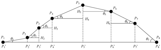
The profile fitting degree is the fitting degree between the compressed trajectory and the original trajectory after the trajectory is linearly approximated to a set of straight lines, which is recorded as . It is affected by the projection angle factor and the projection distance factor. The projection angle factor is a function of the projection length of the original trajectory and the length of the original trajectory. It describes the influence of the angle change of the approximate line segment on the similarity, which is recorded as . The projection distance factor is a function of the projection length of the original trajectory and the distance from the original trajectory to the approximate line segment, which describes the influence of the distance difference between the approximate line segments on the similarity and is recorded as . Figure 1 shows an example of the linear approximation of the original trajectory segment to .
Figure 1.
Schematic diagram of contour fit calculation.
The projection of the original trajectory sub segment is , the projection of the sub segment is , etc., all together constitute the approximate trajectory segment . For the original sub segment , the projection angle factor and the projection distance factor are defined as
where is the distance of the original trajectory segment , is the distance of the projection , and . is the length of the original trajectory sub segment and . We define , and the solution of is based on Helen formula, as shown in Figure 1. The area of is
where is the half perimeter, is the side length , and is .
Obviously, describes the influence of the angle between and on the degree of trajectory approximation. The smaller the angle is, the closer the distance of and is, and tends to 1, while the larger the angle is, tends to 0. In calculation, and are the distance from the two endpoints of the original sub segment to the projection, and takes the smaller value of both, because the difference between them reflects the change of angle, which has been reflected in the calculation of . It can be seen that describes the influence of distance on trajectory approximation. The smaller the distance is, the closer and are, and tends to 1. The larger the distance is, the farther away and are, and tends to 0.
The above calculation of and is applicable to the case where the original trajectory points are on the same side of the compressed trajectory. As shown in Figure 2, the original trajectory points are on both sides of the compressed trajectory. The calculation of and are described as follows.
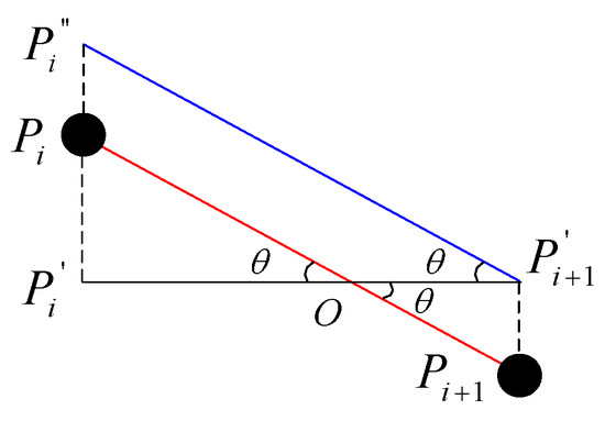
Figure 2.
Original points on both sides of compressed trajectory.
The projection angle factor is defined as the ratio of the projection length to the original sub segment length , and , therefore can reflect the influence of on the trajectory approximation degree, and the calculation of is consistent with the situation of the same side of the trajectory point. However, the original sub segment and projection intersect at point , and the influence of distance on the trajectory similarity has been considered in the calculation of , therefore .
The method of the vector cross product is used to judge whether the projection intersects with the original sub segment . We define
when intersects , and have different signs, and and are the same.
The projection angle factor and distance factor of the original trajectory segment and the approximate trajectory segment can be expressed by the aggregation of the calculation results of each sub segment:
where is the occupancy of the original sub segment in the trajectory segment, which is expressed by its length proportion as
Based on the above calculation, the projection angle factor and distance factor of the whole trajectory can be obtained:
where is the number of segments of the trajectory, and is the occupancy of the original trajectory segment in the trajectory , which can also be expressed by its length proportion.
Finally, the trajectory profile fitting degree is defined as , and are the importance weights of projection angle factor and projection distance factor respectively, and the sum of them is 1.
In summary, the calculation of trajectory profile fitting degree is an aggregation process from sub segment trajectory segment to the whole trajectory, which fully reflects the influence of the angle and distance difference between the approximate trajectory and the original trajectory on the similarity. At the same time, the trajectory profile fitting degree, the projection angle factor and the projection distance factor are all dimensionless, and the values are normalized, thus the applicability is better.
3. The PSOTSC Algorithm
The PSOTSC algorithm is developed in this section where the high-quality segmentation solution is found through particle swarm optimization to achieve better segmentation accuracy and compression rate. First, the overall framework of the algorithm is introduced. Then some key processing links in the algorithm are illustrated in detail, such as particle swarm segmentation optimization method, particle update strategy based on NARJ and the satisfaction judgment method.
3.1. Overall Framework
Trajectory segmentation and compression need to deal with the contradiction or balance between segmentation accuracy and compression rate. Retaining more original trajectory points can bring better similarity, but at the expense of compression rate. On the contrary, excessive pursuit of data compression rate will deteriorate the quality of approximate trajectory, which loses the significance of similar compression. How to optimize the whole effect of trajectory segmentation and compression? The PSOTSC algorithm is developed, which takes the selection of trajectory segmentation feature points as the starting point, and gives full play to the global optimization advantages of PSO. A better target trajectory segmentation and compression solution can be found. Compared with the results obtained by previous algorithms, the new solution can achieve better data compression rate on the same degree of trajectory similarity, i.e., fewer original trajectory points are retained. From another point of view, it can make the compressed trajectory more similar to the original trajectory under the same data compression rate level. The framework of PSOTSC is shown in Algorithm 1.
| Algorithm 1 PSOTSC |
| Input: A set of trajectories |
| Output: A set of compressed trajectories |
| A compression ratio of and a segmentation accuracy of |
| 01: for each do |
| 02: Number of segments ; |
| 03: while do |
| 04: Search optimal segmentation solution ; |
| 05: Calculate the compression ratio and segmentation accuracy of ; |
| 06: Satisfaction judgment ; |
| 07: if |
| 08: break; |
| 09: Increase number of segments ; |
| 10: end while |
| 11: end for |
| 12: Generate a set of compressed trajectories |
| 13: Calculate and of |
First, the input and output of the PSOTSC algorithm should be clarified. In general, the input of the algorithm is the original trajectory data set, which contains many trajectories with large amount of data. The output of the algorithm is the compressed trajectory data set and the evaluation values of data compression rate and segmentation accuracy. The compressed data set contains approximately processed trajectories, which are one-to-one corresponding to the trajectories in the original data set. The key links in the internal processing of the algorithm also have parameters that need to be set by the user, such as the scale of particle swarm, the number of search iterations, etc., which will be described in the subsequent parts of this section. Second, the basic method of trajectory segmentation optimization based on PSO is established (line 4), which can complete the search of the optimal segmentation solution under a fixed number of segments. After that, the fixed number of segments will start from 1 and increase from small to large to search for the corresponding optimal segmentation solution (line 2–10). By calculating and evaluating the compression ratio and segmentation accuracy, a solution meeting the satisfaction requirements will be found (line 5–8). Finally, each trajectory in the original data set is optimized by the above method (line 1–11), the compressed trajectory data set can be generated (line 12), and the compression ratio and segmentation accuracy are given (line 13).
3.2. Particle Swarm Segmentation Optimization
Particle swarm optimization is an evolutionary computation technology based on swarm intelligence. It originated from biologists’ observation and research on the behavior of birds’ foraging process. It has the characteristics of fast calculation speed, good robustness, strong global convergence ability, being easy to understand, easy to realize, etc. In the PSO algorithm, the potential solution of each optimization problem is a bird in the search space, which is called the “particle”. The particle has a fitness value representing whether it is close to the target and a speed value representing its update speed and search direction. The flow of PSO algorithm is shown in Figure 3.
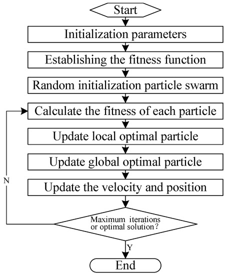
Figure 3.
Basic flow of PSO.
The algorithm is initialized as a group of random particles (random solution) and finds the optimal solution through iteration. The quality of the solution is evaluated by the fitness of the particles. In each iteration, each particle tracks two “optimal particles” to update itself; one is the local optimal particle found by itself, the other is the global optimal particle found by the swarm. The particles follow them to search in the solution space. The advantage of the PSO algorithm is that there is no crossover and mutation operation, and it relies on particle speed and fitness evaluation to complete the search. In the iterative evolution, only the optimal particle transmits information to other particles, therefore the optimization speed is fast and the solution accuracy is high. At the same time, the structure of the algorithm is simple and easy to implement.
method is designed to realize the application of PSO in trajectory segmentation solution search, which is the core of the PSOTSC algorithm shown in Algorithm 2. method needs to solve two key problems: one is how to establish the mapping relationship between the trajectory and the particle; the other is what kind of driving mechanism particles use to update and quickly optimize. To solve the first problem, method maps the compressed trajectory to the particle, which is expressed as a one-dimensional sequence with the same length as the original trajectory. The original trajectory points to be retained and discarded in the sequence are assigned different values. In this way, the problem is simplified, and the process seems simple and straightforward. However, if the length of the original trajectory is very long, it will increase the length of the particle and affect the effect of the algorithm, which leads to the second problem mentioned above. method proposes a NARJ particle update strategy, which can speed up the search of segmentation solution and improve the efficiency of the PSOTSC algorithm. The content of NARJ will be described in detail in Section 3.3.
| Algorithm 2 |
| Input: Trajectory points ordered by time |
| A set of parameters of PSO |
| A threshold of trajectory profile fitting |
| A number of compressed trajectory segments |
| Output: Compressed trajectory points ordered by time |
| 01: Initial particle swarm and velocity , |
| 02: while and do |
| 03: for each do |
| 04: Calculate fitness ; |
| 05: end for |
| 06: Find Current best particle and best fitness with maximum ; |
| 07: Update global best particle and best fitness ; |
| 08: for each do |
| 09: Calculate velocity using ; |
| 10: Update particle based on strategy ; |
| 11: end for |
| 12: end while |
| 13: Construct compressed trajectory ; |
The input of the algorithm is the original trajectory . The basic parameters of PSO include the number of particles , the maximum number of iterations , the learning factor , the maximum and minimum inertia weight and the maximum and minimum velocity .The threshold of trajectory profile fitting degree is , and is the number of trajectory segments. First, the algorithm needs to complete the initialization of particle swarm (line 1), and the premise is to define the particle format. For trajectory , the compressed trajectory is expressed as , where is the segment feature point. Then, the trajectory with segment feature points can be mapped into a sequence of 0 and 1, and the position of 1 in the sequence is . Therefore, we define the particle format as sequence and the length is . is a sequence of 0 and 1 with the length of , and the number of 1 in the sequence is . Random particle means randomizing the position of 1 or the number of 1, representing a random segmentation solution. If the number of trajectory segments is fixed, only the position of 1 needs to be randomized. In order to simplify the calculation, the particle can also be defined as , which is transformed into when the algorithm finally outputs the compressed trajectory.
The algorithm will keep on searching for optimization, as long as the number of iterations is no more than and the trajectory profile fitting degree of the global optimal segmentation solution is less than (line 2). In each iteration, the fitness is calculated for all particles (line 3–5), i.e., the fitting degree of the compressed trajectory represented by the particles and the original trajectory. The fitness function is defined as . The original trajectory TR and particle p are the inputs of this function. The calculation of the function has been described in detail in Section 2.2. The particle with the highest fitness is selected to update the global optimal particle and optimal fitness (line 6–7). Then, the speed of all particles is modified according to the global optimal particle (line 9), and the particle state is updated based on the particle update strategy of NARJ, which will be discussed later. Finally, the algorithm ends the iteration and outputs the compressed trajectory .
3.3. NARJ Particle Update Strategy
In PSO, particle updating is driven by whether the quality of the current particle is close to the quality of the optimal particle. For a particle used to represent a compressed trajectory, the quality of the particle is its profile fitting degree with the original trajectory. The higher the fit, the better the quality of the particle. Therefore, the first problem to be solved is how to evolve a high-quality particle into a better one. A high-quality particle means that the selection of trajectory segmentation feature points is basically reasonable. It only needs to adjust the position of segmentation feature points a little to try to obtain a better solution on the original basis, while excessive or random adjustment of a reasonable segmentation solution may destroy the original balance. Will this fall into the dilemma of local search? What about low-quality particles? These are the next two problems to be solved. The segmentation solution represented by a low-quality particle is not reasonable and needs to be greatly adjusted to try new possibilities. Some segmentation feature points can be selected randomly in the solution and can jump to other positions randomly. Such changes can not only solve the problem of rapid disintegration and the updating of low-quality particles, but also ensure that the PSOTSC algorithm will not fall into local optimization.
Thus, the basic consideration of NARJ particle update strategy is that the segment feature points of high-quality particles are adjusted in their neighborhood, and the probability of evolving into better particles will be larger than that of feature points randomly adjusted. Meanwhile, low-quality particles need to adjust the feature points randomly in a large range to get rid of the current state and try a new segmentation solution to improve the search efficiency. Algorithm 3 gives the of particle update strategy.
| Algorithm 3 |
| Input: A particle and its fitness |
| A neighborhood adjustment span |
| A number of adjusted feature points |
| Output: An evolved particle |
| 01: Select feature points; |
| 02: Evaluate the quality of particle with its fitness ; |
| 03: if is high-quality then |
| /* Neighborhood Adjustment*/ |
| 04: Change the feature points in range; |
| 05: else |
| /* Random Jump */ |
| 06: Change the feature points randomly; |
| 07: end if |
| 08: Set the value of the new points to 1 and the old points to 0; |
| 09: Replace the old particle with the evolved one ; |
The input of the algorithm is particle and its fitness , the neighborhood adjustment span and the number of adjusted feature points . In the evolution process, whether it is neighborhood adjustment or random jump, the segment feature points that change the position are randomly selected (line 1), generally 1~2, so that the search efficiency will not be affected because of the strong randomness. High-quality particles adjust the neighborhood of segment feature points, while low-quality particles adjust the position of segment feature points randomly (line 2–7). The direction of feature point adjustment is random, which can be adjusted forward or backward. In neighborhood adjustment, each feature point is taken as the center, and the feature point position is changed within the range (line 4). The span depends on the total length of the trajectory and the interval of the trajectory points. If the trajectory is long, the interval of the trajectory points is small or the number of points is large, it is necessary to increase the span appropriately to improve the search speed. However, if the interval of trajectory points is larger, and the number of trajectory points is less, the span should be reduced. The algorithm outputs the evolved particle and replaces the original particle .
An example is given to illustrate various situations in the process of particle update, as shown in Figure 4. Only one feature point is adjusted for each evolution, and the neighborhood adjustment span is 1.
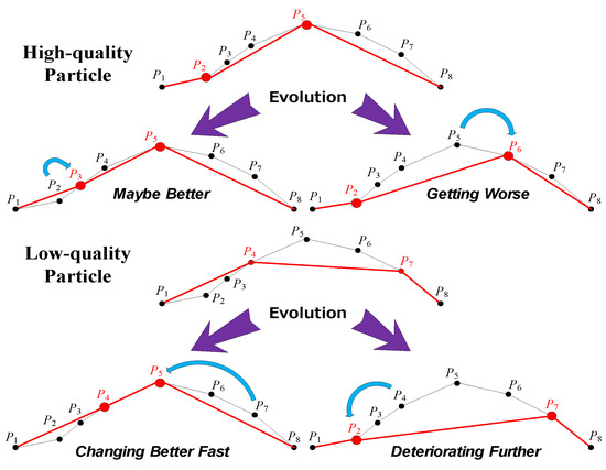
Figure 4.
NARJ particle update strategy.
For a high-quality particle, neighborhood adjustment will produce two possible results. One is the evolution into a better particle, which is obviously the expected result. The other is that the quality becomes worse. The solution is to restore the particle to its original state, so that in the next round of evolution it will try to adjust again based on a good state. In Figure 4, the segment feature points of high-quality particle are and , and adjusting to may lead to a better solution. However, adjusting to will generate a bad solution, so it is necessary to restore to . In the next evolution, will try to adjust to with a certain probability.
For a low-quality particle, the neighborhood adjustment of feature points cannot change the bad state fundamentally, but random jump can bring the possibility of “reversal”. Of course, it may also make the quality worse. In Figure 4, the selection of segment feature point for a low-quality particle is and . After evolution, jumps to , which brings a better solution. The subsequent evolution can adjust the feature points in the neighborhood, such as the high-quality particle. The jump from to further worsens the quality, and the particle will directly enter the next evolution to reflect the randomness and globality.
3.4. Satisfaction Judgment
If the number of segments of the trajectory is 1, i.e., there are no segment feature points except the first and last two points of the trajectory, then the compression ratio of the original trajectory is the best. On the contrary, the segmentation accuracy can be improved by setting as many segmentation feature points as possible and retaining the profile information of the original trajectory, but a certain data compression ratio will be sacrificed. Therefore, we need to find a balance between the number of segments and the accuracy of segmentation. When the satisfaction is reached, we judge that the trajectory segmentation and compression is complete.
Definition 5.
Compression–accuracy contribution rate is the contribution to the trajectory segmentation accuracy at the expense of a certain data compression rate, expressed as
whereis the segmentation accuracy of the trajectory divided intosegments, which is expressed by the trajectory profile fitting degree, andis the data compression ratio after the trajectory is divided intosegments, i.e., the ratio of the number of compressed trajectory points to the number of original trajectory points.
Therefore, the satisfaction decision function can be expressed by the compression–accuracy contribution rate, and the input of the function is the segmentation accuracy and data compression rate of the compression trajectory. When the rate declines continuously, it means that the improvement of segmentation accuracy by sacrificing compression rate is not obvious, and segmentation can be terminated at this time. Users can also set the threshold directly to control the segmentation and compression process according to their own separate requirements for compression rate and segmentation accuracy. When the compression rate or segmentation accuracy reaches the threshold, the process will be stopped, and the satisfaction judgment can be customized.
4. Results and Discussion
4.1. Experimental Setting
We use two real trajectory data sets and one simulated trajectory data set of maneuvering target to verify the effectiveness of the PSOTSC algorithm. The first real data set is the Atlantic hurricane data set from the National Hurricane Center (NHC). It contains all the hurricane movement data from 1851 to 2019. This paper uses all the trajectory data with more than two sampling points, including 1861 trajectories and 51,807 sampling points. The longest trajectory has 133 sampling points, and the average length is 27.8, as shown in Figure 5.
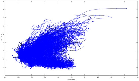
Figure 5.
Hurricane data.
Another real data set is the Starkey ungulate telemetry data set. It contains radio-telemetry locations of elk (Cervus elaphus), mule deer (Odocoileus hemionus) and cattle collected at the Starkey Experimental Forest and Range in northeastern Oregon between 1993 and 1996. We randomly selected 67 targets in the data set, including 102,976 location data. Some trajectories are shown in Figure 6. If each target is represented by only one trajectory, the number of points of the longest one is 4007.
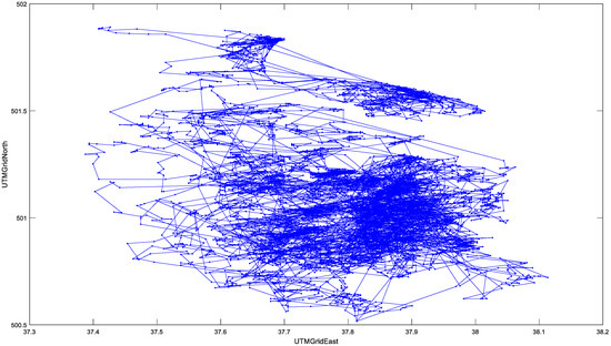
Figure 6.
Ungulate data.
The maneuvering target simulation trajectory data set is based on the maneuvering target tracking simulation model in Section 4.2 of [31], which generates 50 trajectories, each with a length of 50. Figure 7 shows all the trajectories of the simulation data set and some typical trajectories. It can be seen that the trajectories generated by the simulation reflect stronger target motion changes and contain certain randomness, which are in line with the motion characteristics of maneuvering targets in the battlefield.
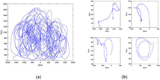
Figure 7.
Trajectory data of maneuvering target simulation: (a) Data set; (b) Typical trajectories.
The PSOTSC algorithm in this paper and the compression algorithms such as DP, TRACLUS and TCSS used for comparison were edited and implemented in MATLAB R2016b. All experiments were carried out on Windows 7 operating system with Intel® Core™ i5-7500, memory size 8 GB.
4.2. Results of Segmentation Accuracy
4.2.1. Real Trajectory Data
We use real data to test the segmentation and compression effect of this algorithm under different numbers of particles and iterations. First, some representative long trajectories in the hurricane data set are segmented. It can be seen from Figure 8 that the segmented trajectories keep the profile features of the original trajectories. By increasing the number of particles from 20 to 50 and the number of iterations from 10 to 20, the segmentation effect is obviously better.
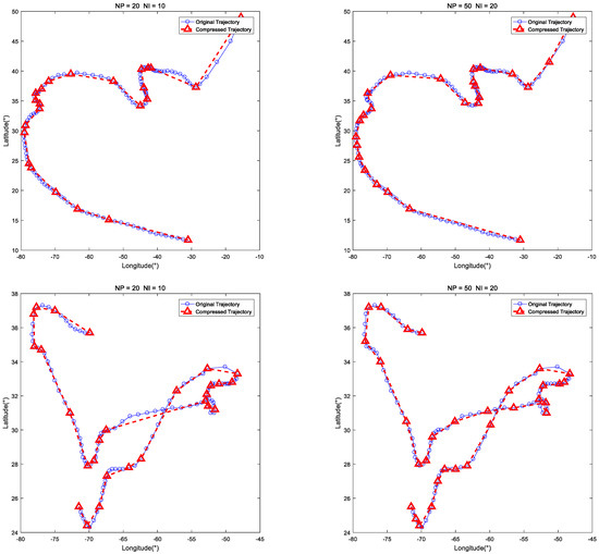
Figure 8.
Segmentation effect of typical hurricane trajectory.
One hundred Monte-Carlo statistical experiments were carried out on the whole hurricane data set to analyze the compression effect of the PSOTSC algorithm; the statistical analysis results are shown in Table 1. Let the mean values of compression rate and accuracy be m_CR and m_AY, respectively, and the standard deviation values be sd_CR and sd_AY. When the segmentation accuracy is controlled at around 98.3%, the overall trajectory compression rate increases with the increase in the number of particles or the number of iterations, which means that the particle swarm optimization can find a better segmentation and compression solution while maintaining the segmentation accuracy. It can be found from the standard deviation results that the standard deviation gradually decreases with the increase in the number of particles and iterations, which indicates that the stability of the optimal search is also increasing.

Table 1.
Performance with different parameter values in hurricane data set experiments.
For ungulate data set, the experiments of the PSOTSC algorithm were also carried out to test the performance. Unlike the experiments for hurricane data set, which uses fixed trajectory segmentation accuracy to find the change of trajectory data compression rate, this time the compression rate is stable at a certain level, i.e., it retains the same number of trajectory points, and finds the change of trajectory segmentation accuracy with the numbers of particles and iterations. One hundred Monte-Carlo statistical experiments were carried out on the whole data set, and the results are shown in Table 2. It can be seen that whether the compression ratio is controlled to 20% or 30%, we can get better trajectory segmentation accuracy with the expansion of particle swarm size and the increase in iteration times. At the same time, we also note that for the ungulate data set, the segmentation accuracy is generally lower than that of the hurricane data set. This is because the trajectories in the ungulate data set have obvious polyline characteristics. Intuitively, the points constituting these polylines should be trajectory feature points, therefore the proportion of redundant data is lower than that of hurricane trajectories, which can be seen from Figure 6.
Table 2.
Performance with different parameter values in ungulate data set experiments.
The advantages of NARJ particle update strategy are verified, and the segmentation accuracy of PSOTSC with NARJ is compared with that of standard PSOTSC with the same number of segments (the same compression ratio), particles and iterations. One hundred Monte-Carlo statistical experiments were carried out on typical trajectories in hurricane and ungulate data sets. The number of particles and iterations is 20 and 10, respectively, and the number of segment feature points increases. The average segmentation accuracy comparison of the two methods under different number of segment feature points is obtained, as shown in Figure 9. When the numbers of particles, iterations and reserved trajectory feature points are the same, the PSOTSC algorithm using NARJ strategy can obtain higher trajectory segmentation accuracy than the standard PSO algorithm. In other words, the neighborhood adjustment and random jump make the particle swarm to search the trajectory segmentation solution in a more reasonable mode.
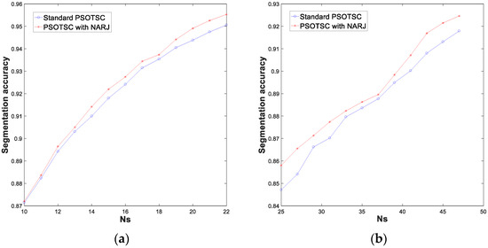
Figure 9.
Performance of NARJ particle update strategy: (a) Hurricane trajectory data set; (b) Ungulate data set.
4.2.2. Maneuvering Target Simulation Data
The profile of hurricane trajectory is relatively simple, and the trajectory generated by the maneuvering target tracking simulation model has more obvious motion changes, including sharp turning, moving along the arc, etc. The segmentation and compression experiments were carried out for typical maneuvering trajectories. As shown in Figure 10, the segmented trajectory generated by PSOTSC can fit the original trajectory profile well.
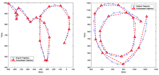
Figure 10.
Segmentation effect of maneuvering target simulation.
4.3. Results of Algorithm Comparison
Compared with DP, TRACLUS and TCSS typical segmentation and compression algorithms, the advantage of the PSOTSC algorithm is verified on real trajectory data set and maneuvering target simulation data set. The experimental results are shown in Figure 11. In the experiment of real trajectory data set, the number of initialization particles is 15 and the maximum number of iterations is 5. The DP algorithm needs to adjust the distance threshold to obtain the optimal segmentation, and the threshold sampling point in the experiment is . The segmentation algorithm in TRACLUS will be affected by trajectory scaling, and different scaling ratios will affect the segmentation accuracy. The scaling ratio in the experiment is . The segmentation accuracy of the TCSS algorithm is affected by the angle threshold setting, and the angle threshold setting in the experiment is . In the experiment of maneuvering target simulation data set, the parameters , and still need to be adjusted.
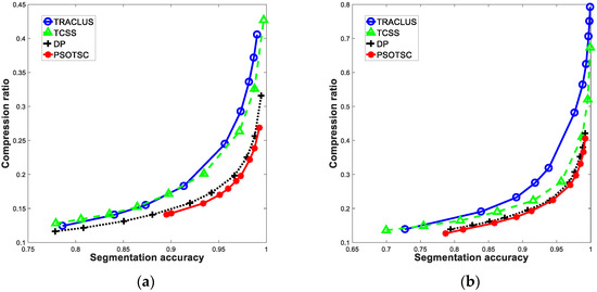
Figure 11.
Comparison results of segmentation accuracy and compression ratio: (a) Real trajectory data set; (b) Maneuvering target simulation data set.
As shown in Figure 11, the segmentation accuracy compression ratio curve obtained by the PSOTSC method is at the bottom of all comparison method curves, which can not only show that the PSOTSC method can achieve the lowest compression ratio under the same segmentation accuracy level, but can also show that the PSOTSC method can obtain the highest segmentation accuracy under the same compression ratio requirements. Therefore, this method has advantages over typical methods in segmentation accuracy and compression ratio.
5. Conclusions
In this paper, we discussed the technical route of swarm intelligence algorithm to solve the problem of trajectory segmentation and compression, and propose a PSOTSC algorithm based on particle swarm optimization, which transforms the trajectory segmentation problem into the global optimization problem of segment feature points. The PSOTSC algorithm makes the selection of feature points more accurate and improves the accuracy of trajectory segmentation. Meanwhile, the particle update strategy based on NARJ is established, which can effectively improve the search efficiency of trajectory segmentation solution. Compared with the standard particle swarm optimization method, the trajectory segmentation accuracy is higher under the same compression rate. The effectiveness of the proposed method is verified by real data set and simulation data set. The experimental results show that the PSOTSC algorithm can obtain a satisfactory segmentation and compression solution, and the compression ratio and segmentation accuracy are better than those in typical algorithms, such as DP, TRACLUS, and TCSS. Because the PSOTSC algorithm belongs to the global-oriented segmentation and compression method, the computational complexity will increase greatly when facing the long trajectory with more sampling points. In future, we will focus on reducing the time complexity of the algorithm and consider the long trajectory pre-segmentation, search by segment and synthesis optimization to expand the applicability of the algorithm. The PSOTSC algorithm takes advantage of SI to obtain the optimization solution through global search, but the problem inherent in the global search algorithm is the large computation. An intuitive and easy solution is that long trajectories can be divided into several short trajectories to search and optimize respectively and then complete the aggregation and overall optimization, but there may be some better way to deal with this issue. Therefore, the next research will focus on the long trajectory global segmentation and compression based on SI methods.
Author Contributions
Conceptualization, Zhihong Ouyang; Formal analysis, Zhihong Ouyang; Investigation, Zhihong Ouyang; Resources, Lei Xue; Supervision, Lei Xue; Visualization, Da Li; Writing—original draft, Zhihong Ouyang; Writing—review and editing, Feng Ding. All authors have read and agreed to the published version of the manuscript.
Funding
This research and the APC were funded by L.X.
Conflicts of Interest
The authors declare no conflict of interest.
References
- Kontopoulos, I.; Makris, A.; Tserpes, K. A Deep Learning Streaming Methodology for Trajectory Classification. ISPRS Int. J. Geo-Inf. 2021, 10, 250. [Google Scholar] [CrossRef]
- Hachem, F.; Damiani, M.L. Periodic stops discovery through density-based trajectory segmentation. In Proceedings of the SIGSPATIAL’18, Seattle, WA, USA, 6 November 2018. [Google Scholar]
- Bin, C.; Gu, T.; Sun, Y.; Chang, L. A personalized POI route recommendation system based on heterogeneous tourism data and sequential pattern mining. Multimed. Tools Appl. 2019, 78, 35135–35156. [Google Scholar] [CrossRef]
- Xu, J.Q.; Guting, R.H.; Gao, Y.J. Continuous k nearest neighbor queries over large multi-attribute trajectories: A systematic approach. Geoinformatica 2018, 22, 723–766. [Google Scholar] [CrossRef]
- Wang, Y.; Qin, K.; Chen, Y.; Zhao, P. Detecting anomalous trajectories and behavior patterns using hierarchical clustering from taxi GPS data. Int. J. Geo-Inf. 2018, 7, 25. [Google Scholar] [CrossRef] [Green Version]
- Yu, Q.; Luo, Y.; Chen, C.; Chen, S. Trajectory similarity clustering based on multi-feature distance measurement. Appl. Intell. 2019, 49, 2315–2338. [Google Scholar] [CrossRef]
- Cai, L.; Jiang, F.; Zhou, W.; Li, K. Design and Application of an Attractiveness Index for Urban Hotspots Based on GPS Trajectory Data. IEEE Access 2018, 6, 55976–55985. [Google Scholar] [CrossRef]
- Makris, A.; Kontopoulos, I.; Alimisis, P.; Tserpes, K. A Comparison of Trajectory Compression Algorithms Over AIS Data. IEEE Access 2021, 9, 92516–92530. [Google Scholar] [CrossRef]
- Makris, A.; da Silva, C.L.; Bogorny, V.; Alvares, L.O.; Macedo, J.A.; Tserpes, K. Evaluating the effect of compressing algorithms for trajectory similarity and classification problems. GeoInformatica 2021, 25, 679–711. [Google Scholar] [CrossRef]
- Leichsenring, Y.E.; Baldo, F. An evaluation of compression algorithms applied to moving object trajectories. Int. J. Geogr. Inf. Sci. 2019, 34, 539–558. [Google Scholar] [CrossRef]
- Sun, P.H.; Xia, S.X.; Yuan, G.; Li, D.X. An overview of moving object trajectory compression algorithms. Math. Probl. Eng. 2016, 3, 1–13. [Google Scholar] [CrossRef] [Green Version]
- Douglas, D.H.; Peucker, T.K. Algorithms for the reduction of the number of points required to represent a digitized line or its caricature. Cartogr. Int. J. Geogr. Inf. Geovis. 1973, 10, 112–122. [Google Scholar] [CrossRef] [Green Version]
- Liu, J.; Li, H.; Yang, Z.; Wu, K.; Liu, Y.; Liu, R.W. Adaptive Douglas-Peucker Algorithm with Automatic Thresholding for AIS-Based Vessel Trajectory Compression. IEEE Access 2019, 7, 150677–150692. [Google Scholar] [CrossRef]
- Zhao, L.B.; Shi, G.Y. A method for simplifying ship trajectory based on improved Douglas-Peucker algorithm. Ocean Eng. 2018, 166, 37–46. [Google Scholar] [CrossRef]
- Zhao, L.B.; Shi, G.Y. A trajectory clustering method based on Douglas-Peucker compression and density for marine traffic pattern recognition. Ocean. Eng. 2019, 172, 456–467. [Google Scholar] [CrossRef]
- Huang, Y.; Li, Y.; Zhang, Z.; Liu, R.W. GPU-Accelerated Compression and Visualization of Large-Scale Vessel Trajectories in Maritime IoT Industries. IEEE Internet Things J. 2020, 7, 10794–10812. [Google Scholar] [CrossRef]
- Mou, J.M.; Chen, P.F.; He, Y.X.; Zhang, X.J.; Zhu, J.F.; Rong, H. Fast self-tuning spectral clustering algorithm for AIS ship trajectory. J. Harbin Eng. Univ. 2018, 39, 428–431. [Google Scholar]
- Zhu, J.; Huang, C.; Yang, M.; Fung, G.P.C. Context-based prediction for road traffic state using trajectory pattern mining and recurrent convolutional neural networks. Inf. Sci. 2018, 473, 190–201. [Google Scholar] [CrossRef]
- Zhao, Y.; Shang, S.; Wang, Y.; Zheng, B.; Nguyen, Q.V.H.; Zheng, K. REST: A reference-based framework for spatio-temporal trajectory compression. In Proceedings of the 24th ACM SIGKDD Conference on Knowledge Discovery and Data Mining, London, UK, 19–23 August 2018; pp. 2797–2806. [Google Scholar]
- Roniel, S.D.S.; Azzedine, B.; Antonio, A.F.L. Vehicle Trajectory Similarity: Models, Methods, and Applications. ACM Comput. Surv. 2020, 53, 1–32. [Google Scholar]
- Zheng, K.; Zhao, Y.; Lian, D.; Zheng, B.; Liu, G.; Zhou, X. Reference-Based Framework for Spatio-Temporal Trajectory Compression and Query Processing. IEEE Trans. Knowl. Data Eng. 2020, 32, 2227–2240. [Google Scholar] [CrossRef]
- Han, Y.; Sun, W.; Zheng, B. COMPRESS: A comprehensive framework of trajectory compression in road networks. ACM Trans. Database Syst. 2017, 42, 11. [Google Scholar] [CrossRef]
- Jin, J.L.; Zhou, W.J.; Bai, C. Trajectory segmentation algorithm based on behavior pattern. J. Signal Process. 2020, 36, 2074–2084. [Google Scholar]
- Cai, G.; Lee, K.; Lee, I. Mining Semantic Trajectory Patterns from Geo-Tagged Data. J. Comput. Sci. Technol. 2018, 33, 849–862. [Google Scholar] [CrossRef]
- Cai, G.; Lee, K.; Lee, I. Mining Mobility Patterns from Geotagged Photos Through Semantic Trajectory Clustering. Cybern. Syst. 2018, 49, 234–256. [Google Scholar] [CrossRef]
- Wei, Z.; Xie, X.; Zhang, X. AIS trajectory simplification algorithm considering ship behaviours. Ocean. Eng. 2020, 216, 108086. [Google Scholar] [CrossRef]
- Giannis, F.; Kostas, P.; Alexander, A. Optimizing Vessel Trajectory Compression. In Proceedings of the 21st IEEE International Conference on Mobile Data Management, Versailles, France, 3 July 2020; pp. 2429–2436. [Google Scholar]
- Liang, M.; Liu, R.W.; Li, S.; Xiao, Z.; Liu, X.; Lu, F. An unsupervised learning method with convolutional auto-encoder for vessel trajectory similarity computation. Ocean. Eng. 2021, 225, 108803. [Google Scholar] [CrossRef]
- Etemad, M.; Soares, A.; Etemad, E.; Rose, J.; Torgo, L.; Matwin, S. SWS: An unsupervised trajectory segmentation algorithm based on change detection with interpolation kernels. GeoInformatica 2020, 25, 269–289. [Google Scholar] [CrossRef]
- Junior, A.S.; Times, V.C.; Renso, C.; Matwin, S.; Cabral, L.A. A Semi-Supervised Approach for the Semantic Segmentation of Trajectories. In Proceedings of the 19th IEEE International Conference on Mobile Data Management, Aalborg, Denmark, 26–28 June 2018; pp. 145–154. [Google Scholar]
- Fazzinga, B.; Flesca, S.; Furfaro, F.; Masciari, E. RFID-data compression for supporting aggregate queries. ACM Trans. Database Syst. 2013, 38, 1–45. [Google Scholar] [CrossRef]
- Fazzinga, B.; Flesca, S.; Furfaro, F.; Masciari, E. Efficient and effective RFID data warehousing. In Proceedings of the 2009 International Database Engineering & Applications Symposium, Cetraro, Italy, 16–18 September 2009; pp. 251–258. [Google Scholar]
- Hershberger, J.E.; Snoeyink, J. Speeding up the douglas-peucker line-simplification algorithm. In International Symposium on Spatial Data Handling; Springer: Berlin/Heidelberg, Germany, 1992; pp. 134–143. [Google Scholar]
- Meratnia, N.; Rolf, A. Spatiotemporal compression techniques for moving point objects. In Proceedings of the Advances in Database Technology (EDBT 2004); Springer: Berlin/Heidelberg, Germany, 2004; pp. 765–782. [Google Scholar]
- Muckell, J.; Olsen, P.W.; Hwang, J.H.; Lawson, C.T.; Ravi, S.S. Compression of trajectory data: A comprehensive evaluation and new approach. Geoinformatica 2014, 18, 435–460. [Google Scholar] [CrossRef]
- Muckell, J.; Hwang, J.H.; Lawson, C.T.; Ravi, S.S. Algorithms for compressing GPS trajectory data: An empirical evaluation. In Proceedings of the 18th SIGSPATIAL International Conference on Advances in Geographic Information Systems, San Jose, CA, USA, 2–5 November 2010; pp. 402–405. [Google Scholar]
- Bellman, R.E. On the approximation of curves by line segments using dynamic programming. CACM 1961, 4, 284. [Google Scholar] [CrossRef]
- Potamias, M.; Patroumpas, K.; Sellis, T. Sampling trajectory streams with spatiotemporal criteria. In Proceedings of the 18th SIGSPATIAL International Conference on Scientific and Statistical Database Management (SSDBM’06), Vienna, Austria, 3–5 July 2006; pp. 275–284. [Google Scholar]
- Liu, J.; Zhao, K.; Sommer, P.; Shang, S.; Kusy, B.; Jurdak, R. Bounded quadrant system: Error-bounded trajectory compression on the go. In Proceedings of the 31st IEEE International Conference on Data Engineering, Seoul, Korea, 13–17 April 2015; pp. 987–998. [Google Scholar]
- Chen, C.; Ding, Y.; Xie, X.; Zhang, S.; Wang, Z.; Feng, L. TrajCompressor: An Online Map-matching-based Trajectory Compression Framework Leveraging Vehicle Heading Direction and Change. IEEE Trans. Intell. Syst. 2019, 21, 1–15. [Google Scholar] [CrossRef]
- Lee, J.G.; Han, J.; Whang, K.Y. Trajectory clustering: A partition-and-group framework. In Proceedings of the 2007 ACM SIGMOD International Conference on Management of Data, Beijing, China, 12–14 June 2007; pp. 593–604. [Google Scholar]
- Lee, J.G.; Han, J.; Li, X. Trajectory outlier detection: A partition-and-detect framework. In Proceedings of the 24th International Conference on Data Engineering, Cancun, Mexico, 7–12 April 2008; pp. 140–149. [Google Scholar]
- Lee, J.G.; Han, J.; Li, X.; Gonzalez, H. TraClass: Trajectory classification using hierarchical region-based and trajectory-based clustering. Proc. VLDB Endow. 2008, 1, 1081–1094. [Google Scholar] [CrossRef]
- Lee, J.G.; Han, J.; Li, X. A unifying framework of mining trajectory patterns of various temporal tightness. IEEE Trans. Knowl. Data Eng. 2015, 27, 1478–1490. [Google Scholar] [CrossRef]
- Yuan, H.; Qian, Y.; Yang, R. Research on GPS- trajectory-based personalization POI and path mining. Syst. Eng. Theory Pract. 2015, 35, 1276–1282. [Google Scholar]
- Liu, X.; Dong, L.; Shang, C.; Wei, X. An improved high-density sub trajectory clustering algorithm. IEEE Access 2020, 8, 46041–46054. [Google Scholar] [CrossRef]
- Zhang, H.F.; Pi, D.C.; Dong, Y.L. iBTC: A trajectory clustering algorithm based on Isolation Forest. Comput. Sci. 2019, 46, 251–259. [Google Scholar]
- Guan, Y.; Xia, S.X.; Zhang, L.; Zhou, Y. Trajectory clustering algorithm based on structural similarity. J. Commun. 2011, 32, 103–110. [Google Scholar]
- Yuan, G.; Xia, S.; Zhang, L.; Zhou, Y.; Ji, C. An efficient trajectory-clustering algorithm based on an index tree. Trans. Inst. Meas. Control. 2011, 34, 850–861. [Google Scholar] [CrossRef]
- Cheng, L.; Raymond, C.W.W.; Jagadish, H.V. Direction-preserving trajectory simplification. Proc. VLDB Endow. 2013, 6, 949–960. [Google Scholar]
- Kennedy, J.; Eberhart, R.; Shi, Y.H. Swarm Intelligence; Morgan Kaufmann Publishers: San Mateo, CA, USA, 2001. [Google Scholar]
- Engelbrecht, A.P. Computational Intelligence: An Introduction; Wiley: Hoboken, NJ, USA, 2007. [Google Scholar]
- Hussain, K.; Salleh, M.N.M.; Cheng, S.; Shi, Y.H. Metaheuristic research: A comprehensive survey. Artif. Intell. Rev. 2019, 52, 2191–2233. [Google Scholar] [CrossRef] [Green Version]
- Houssein, E.H.; Gad, A.G.; Hussain, K.; Suganthan, P.N. Major Advances in Particle Swarm Optimization: Theory, Analysis, and Application. Swarm Evol. Comput. 2021, 63, 1–39. [Google Scholar] [CrossRef]
- Pace, F.; Santilano, A.; Godio, A. A Review of Geophysical Modeling Based on Particle Swarm Optimization. Surv. Geophys. 2021, 42, 1–45. [Google Scholar] [CrossRef] [PubMed]
- Kennedy, J.; Eberhart, R. Particle swarm optimization. In Proceedings of the International Conference on Neural Networks (ICNN’95), Perth, WA, Australia, 27 November–1 December 1995; pp. 1942–1948. [Google Scholar]
- Wang, D.S.; Tan, D.; Liu, L. Particle swarm optimization algorithm: An overview. Soft Comput. 2018, 22, 387–408. [Google Scholar] [CrossRef]
- Jin, X.; Liu, S.; Baret, F.; Hemerlé, M.; Comar, A. Estimates of plant density of wheat crops at emergence from very low altitude UAV imagery. Remote Sens. Environ. 2017, 198, 105–114. [Google Scholar] [CrossRef] [Green Version]
- Poli, R. Analysis of the Publications on the Applications of Particle Swarm Optimisation. J. Artif. Evol. Appl. 2008, 2008, 1–10. [Google Scholar] [CrossRef]
- Adhan, S.; Bansal, P. Applications and variants of particle swarm optimization: A review. Int. J. Electron. Electr. Comput. Syst. 2017, 6, 215–223. [Google Scholar]
- Ratnaweera, A.; Halgamuge, S.K.; Watson, H.C. Self-organizing hierarchical particle swarm optimizer with time-varying acceleration coefcients. IEEE Trans. Evol. Comput. 2004, 8, 240–255. [Google Scholar] [CrossRef]
- Perez, R.E.; Behdinan, K. Particle swarm approach for structural design optimization. Comput. Struct. 2007, 85, 1579–1588. [Google Scholar] [CrossRef]
- Zhan, Z.H.; Zhang, J.; Li, Y.; Chung, H.S. Adaptive particle swarm optimization. IEEE Trans. Syst. Man Cybern. Part B 2009, 39, 1362–1381. [Google Scholar] [CrossRef] [PubMed] [Green Version]
- Gou, J.; Lei, Y.X.; Guo, W.P.; Wang, C.; Cai, Y.Q.; Luo, W. A novel improved particle swarm optimization algorithm based on individual diference evolution. Appl. Soft Comput. 2017, 57, 468–481. [Google Scholar] [CrossRef]
- Coello, C.A.C.; Pulido, G.T.; Lechuga, M.S. Handling multiple objectives with particle swarm optimization. IEEE Trans. Evol. Comput. 2004, 8, 256–279. [Google Scholar] [CrossRef]
- Margarita, R.-S.; Carlos, A.C.C. Multi-objective particle swarm optimizers: A survey of the state-of-the-art. Int. J. Comput. Intell. Res. 2006, 2, 287–308. [Google Scholar]
- Tripathi, P.K.; Bandyopadhyay, S.; Pal, S.K. Multi-Objective Particle Swarm Optimization with time variant inertia and acceleration coefficients. Inf. Sci. 2007, 177, 5033–5049. [Google Scholar] [CrossRef] [Green Version]
- Li, T.; Sun, S.; Corchado, J.M.; Siyau, M.F. A particle dyeing approach for track continuity for the SMC-PHD filter. In Proceedings of the 17th International Conference on Information Fusion, Salamanca, Spain, 7–10 July 2014. [Google Scholar]
Publisher’s Note: MDPI stays neutral with regard to jurisdictional claims in published maps and institutional affiliations. |
© 2021 by the authors. Licensee MDPI, Basel, Switzerland. This article is an open access article distributed under the terms and conditions of the Creative Commons Attribution (CC BY) license (https://creativecommons.org/licenses/by/4.0/).