A Hierarchical Spatial Network Index for Arbitrarily Distributed Spatial Objects

Abstract

The range query is one of the most important query types in spatial data processing. Geographic information systems use it to find spatial objects within a user-specified range, and it supports data mining tasks, such as density-based clustering. In many applications, ranges are not computed in unrestricted Euclidean space, but on a network. While the majority of access methods cannot trivially be extended to network space, existing network index structures partition the network space without considering the data distribution. This potentially results in inefficiency due to a very skewed node distribution. To improve range query processing on networks, this paper proposes a balanced Hierarchical Network index (HN-tree) to query spatial objects on networks. The main idea is to recursively partition the data on the network such that each partition has a similar number of spatial objects. Leveraging the HN-tree, we present an efficient range query algorithm, which is empirically evaluated using three different road networks and several baselines and state-of-the-art network indices. The experimental evaluation shows that the HN-tree substantially outperforms existing methods.

1. Introduction

Spatial databases have grown dramatically in size due to newly emerging data sources attributed to the low-cost sensor and smartphone applications [1,2] and respective crowdsourcing efforts [3,4]. Spatial data also play a significant role in improving our understanding of complex urban systems [5]. Efficiently managing such structured big geospatial data requires equally efficient access methods in support of query processing, data analytics, and emerging location-based service applications. Scientists and users are interested in aspects of the data, for example, bike sharing services may need to analyze the number of bikes available within 3 km of a subway station or a detective may analyze user trajectories to identify potential witnesses within a 100 m range of a crime scene. For this purpose, the range query is a canonical spatial query type since it answers the questions as to which Spatial Objects (SO) lie within a certain distance from a query point. The range query is also used by data mining applications such as density-based clustering [6]. We note that, in our work, we assume that spatial objects are points, such as the locations of points of interests or individual observed locations of users. We do not consider the case where spatial objects are lines or polylines the represent entire trajectories.

Since Guttman proposed the R-tree [7] in 1984, a plethora of indexing methods have been proposed in support of range queries as they are also related to different fields and disciplines [8,9] including for example spatiotemporal data [10]. However, the underlying assumption for most indices is that space is unconstrained and the distance between two objects can be calculated as the Euclidean distance [11,12,13,14]. In many applications, space is constrained and SOs are not uniformly distributed. This scenario makes traditional indexing methods inefficient and provides room for improvement since (i) bounding box approximations may arbitrarily partition networks and the metric space they create; (ii) bounding boxes may also index mostly empty space when it comes to networks; and  (iii) the Euclidean distance may differ greatly from network distance, e.g., two objects separated by a river.

Considering the network nature of the data—indexing and query processing can lead to improved data management solutions [15,16,17,18,19,20,21,22]. These methods decompose the road network into a series of sub-networks based on the specific heuristic, and then index the spatial objects on each sub-network with the specific index. With the exception of [16], one of the main shortcomings of these methods is the way the network space is partitioned, they do not consider the data distribution and just involve network topology, which may lead to inefficient query processing. The approach of [16] is tailored to a specific type of path query and it is not trivial to generalize these solutions to other queries. Therefore, in this paper, we focus on a range query on the road network, the main challenges are twofold: (1) how to partition the road network considering both network topology and the data distribution without data loss; and (2) how to construct the index based on the hierarchical partitioning results to efficiently support range queries.

To this end, this paper proposes a novel spatial index for SOs on road networks called the Hierarchical Network tree (HN-tree). This index employs a hierarchical partitioning of the road network based on both network topology and the data distribution. Using the HN-tree, we devise algorithms to support range queries on networks. Note that our work focuses only on efficiency, as we require to return exact (correct) range query answers (without any approximation). Since state-of-the-art methods, as well as ours, return the correct results (not approximation), there is no notion of effectiveness in our paper. We conduct experiments using three different datasets to verify the efficiency and performance compared to other indices and range query algorithms. More specifically, our contributions can be summarized as follows:

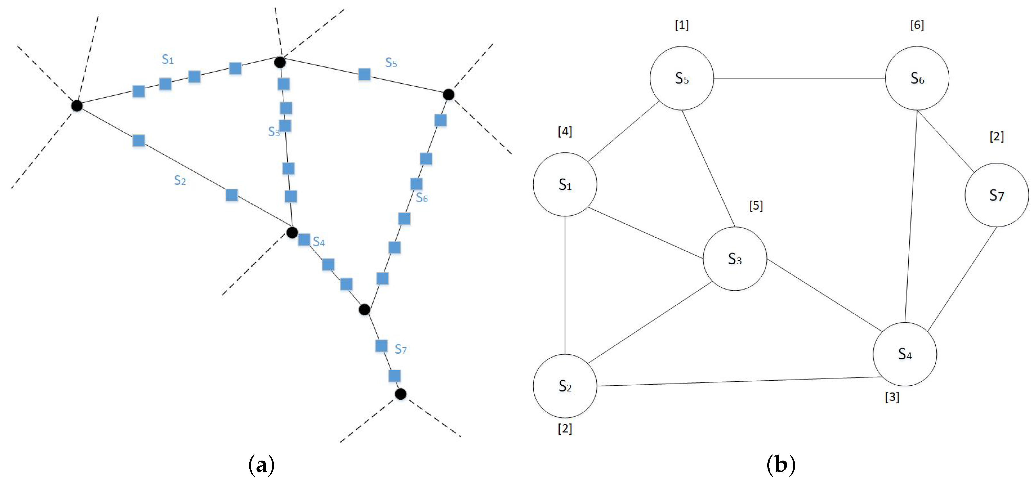
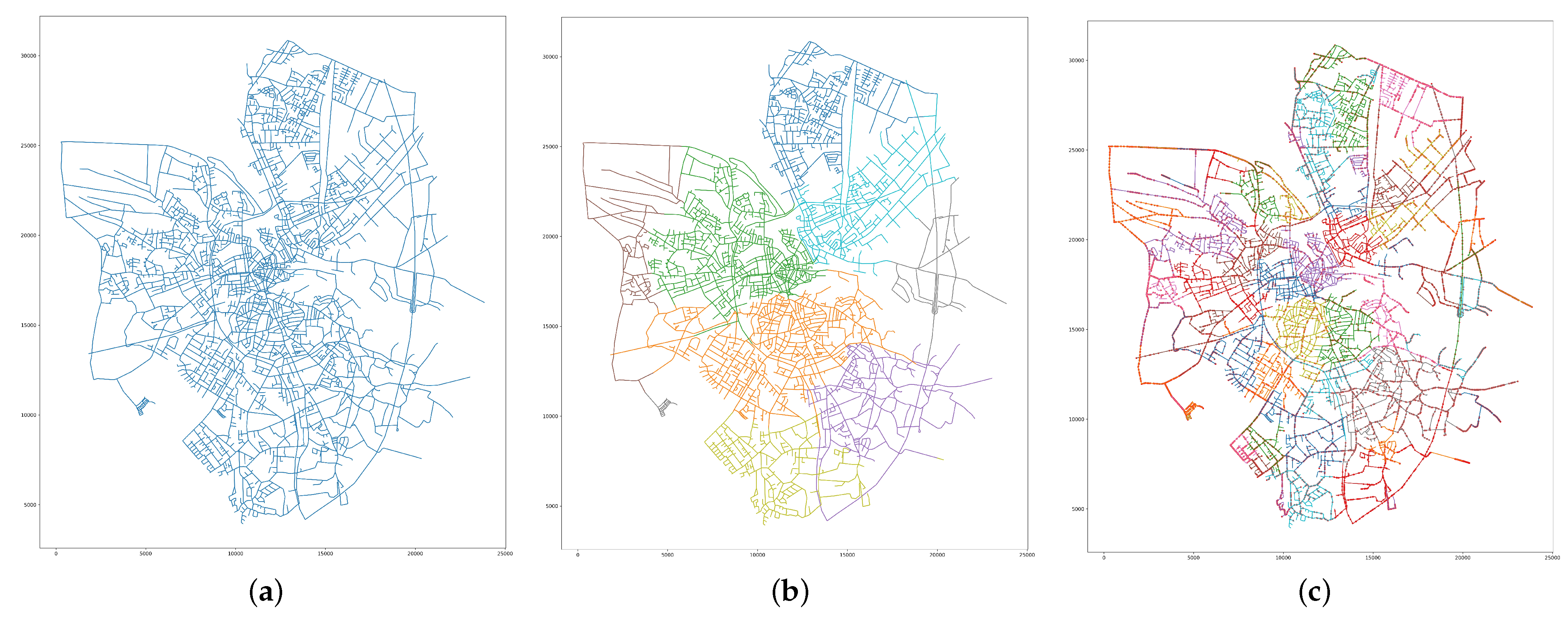
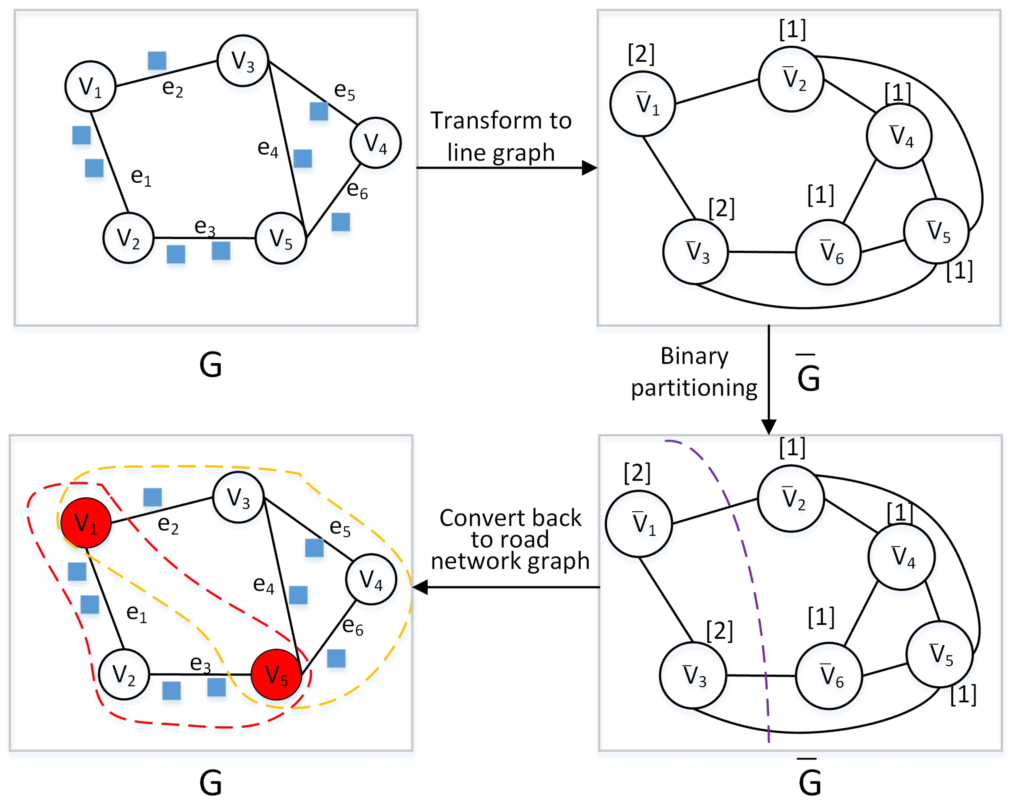
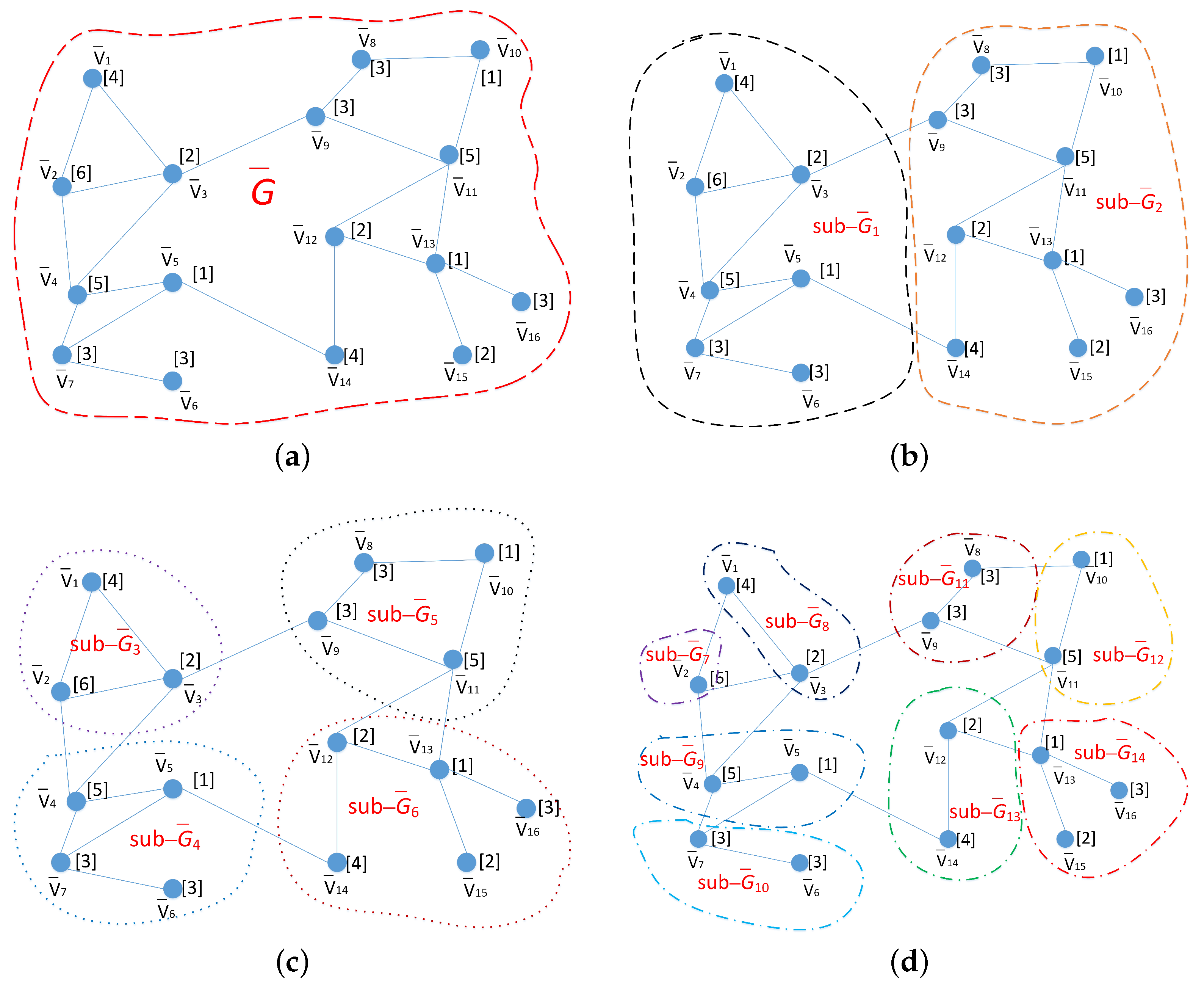
• We propose a hierarchical graph partitioning algorithm that preserves the edges between partitions. The main idea of this algorithm is to (1) transform the network into a line graph (switching nodes and edges); (2) utilize a traditional graph partitioning algorithm on the line graph; and (3) map the resulting partitions back to their spatial network representation.
• Leveraging this graph partitioning, we propose a novel hierarchical network index, the HN-tree, which recursively partitions the network based on the distribution of SOs.
• We devise a range query processing algorithm using our proposed HN-tree.
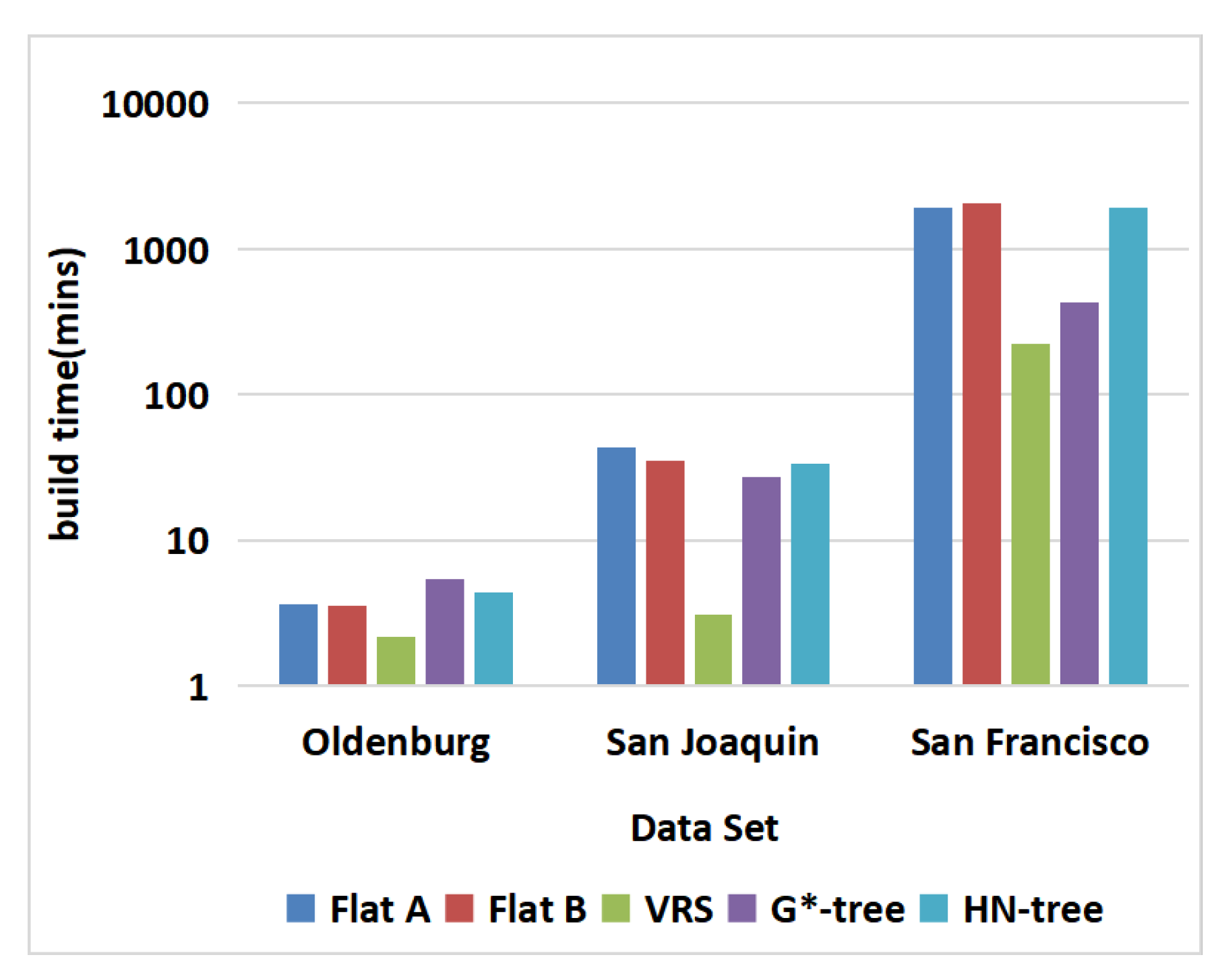
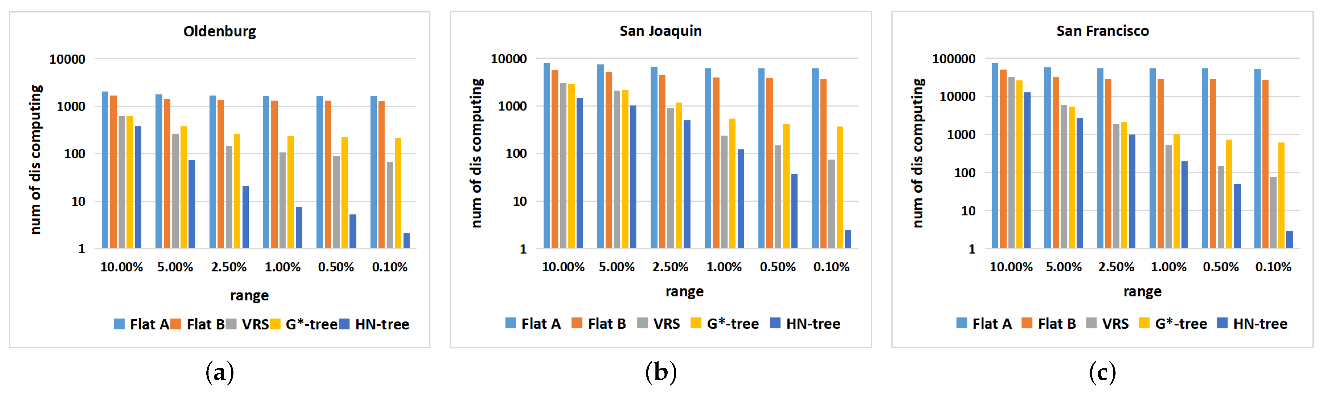
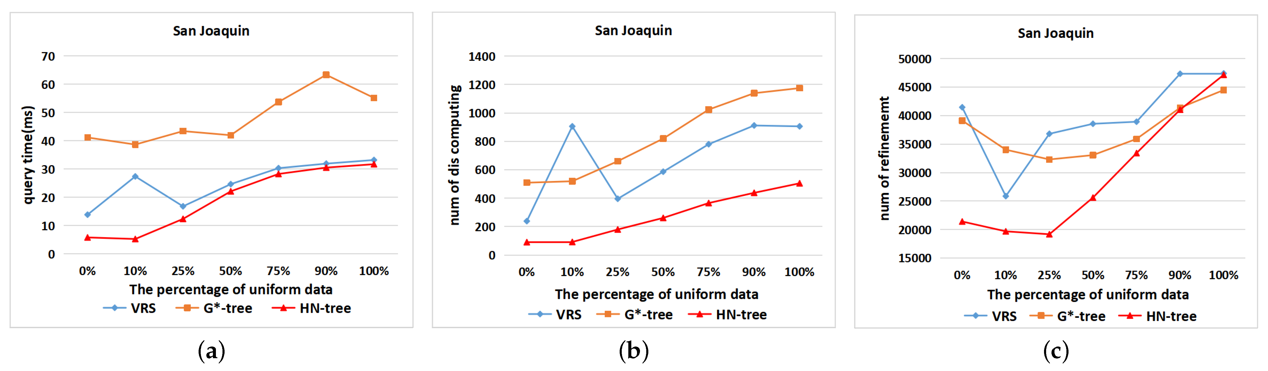
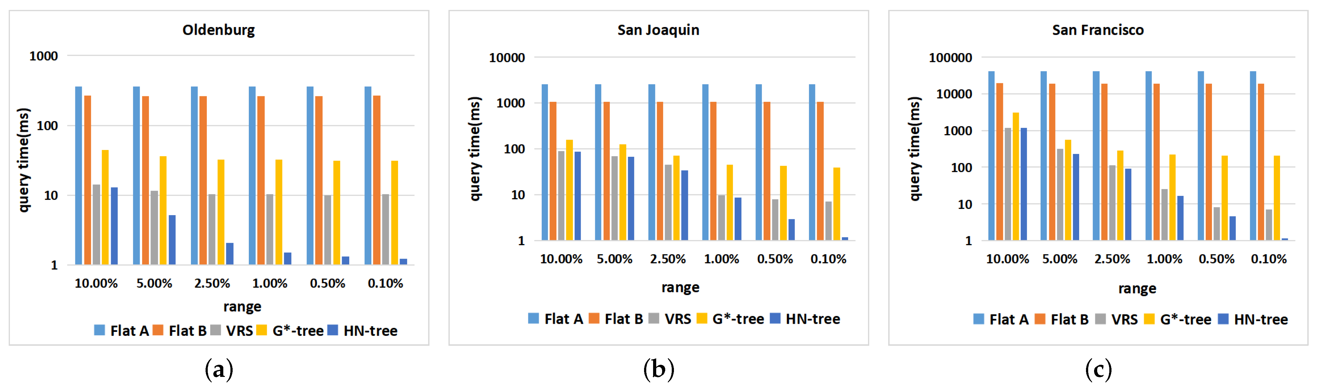
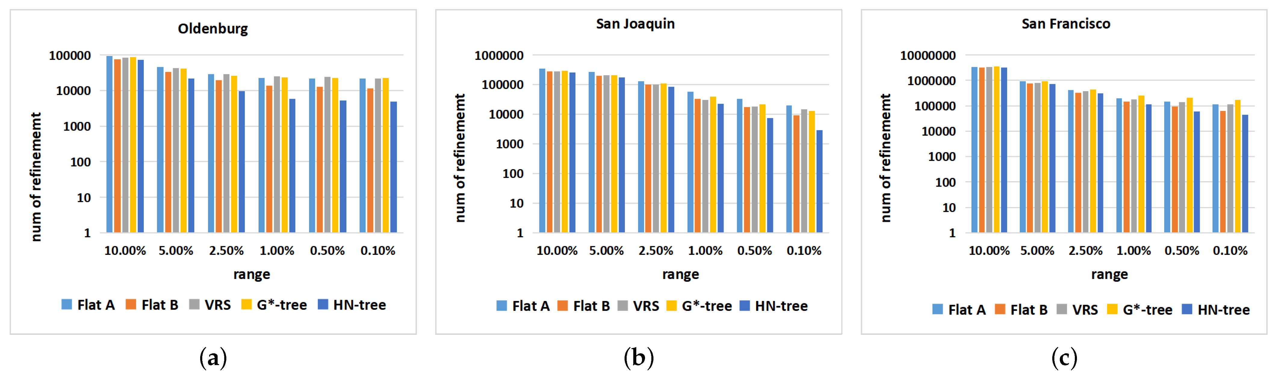
• Experimental results for three different datasets show that this HN-tree based method greatly outperforms state-of-the-art range query and indexing methods in terms of efficiency.

The rest of the paper is organized as follows. Section 2 summarizes the related work. Section 3 presents the network model and network partitioning algorithm. The HN-tree structure is described in Section 4 and Section 5 presents the query processing algorithm. Section 6 details experimental results and discusses performance. Finally, Section 7 concludes and provides directions for future work.

2. Related Work

According to [23], SOs can be divided into three categories based on their distribution in two-dimensional space: distributed freely (e.g., birds in the sky), distributed in constrained regions (e.g., tigers in mountainous areas), and distributed on a spatial network, such as a transportation networks (e.g., bikes on road networks). While unconstrained and constrained SOs largely rely on the same type of query processing and utilize the same access methods, movement on networks differs significantly. A plethora of exiting works have addressed these issues and what follows is a discussion of representative methods in relation to these challenges.

A category of existing work is based on free space using traditional spatial access methods such as the R-tree [7] and the k-d tree [24]. The R-tree [7], which arguably is the most prominent spatial access method, and its variants, e.g., the R*-tree [25] and others [26,27] performance best for range queries in free space. However, when indexing objects on networks, the resulting dead space of their minimum-bounding rectangle (MBR) degrades the performance of such clustering-based methods [18]. Here, Incremental Euclidean Restriction (IER) [18] uses an R-tree to process objects on networks and the experimental results demonstrate that the performance is worse than incremental network expansion (INE) [18] and Voronoi-based range search algorithm (VRS) [17]. To address the dead space problem, a number of works address spatial queries on road networks, i.e., range queries [18,28], continuous range queries [29], k-nearest neighbor [19,28], continuous k-nearest neighbor [30], and shortest path queries [31,32]. These works improve the performance for specific queries, but these methods do not consider the data distribution. Specifically, works such as [29,30] view each edge as a unit, and a road network is partitioned into an equal number of edges. An example here is the G-tree [19] and G*-tree [28], which is a hierarchical tree structure. Our HN-tree shares similarities when it comes to index construction, but differs with respect partitioning (relying on data distribution and network topology) and its range query algorithm. The HN-tree utilizes a line graph, a transformation of the original spatial graph that represents edges as nodes and vice versa, to partition the network. The G-tree and G*-tree use the road network directly. The resulting HN-tree partitions are overlapping and some nodes are shared between partitions. This guarantees that all edges belong to one partition, which is not the case for the G-tree. Figure 1 presents an example detailing partitioning and HN-tree constructions. Given that our dataset consists of spatial objects on network links, this distinction is important. As such, the query processing algorithms of one method cannot directly be applied to the other as the G-tree focuses on kNN and shortest path distances rather than on range queries.

In [18], the incremental euclidean restriction (IER) and the incremental network expansion (INE) take advantage of location and connectivity to prune the search space. Utilizing the R-tree, the IER initially performs a range query and returns the subset within the diameter range r, which serves as the upper bound of the search area. In the refinement step, the actual objects are retrieved based on the shortest path distance. The INE algorithm first computes the set of qualifying network segments (using paths branching out from the query location) and then retrieves the data points falling on these segments. Although more efficient than the Euclidean range search, compared to our method, they produce a high number of false positives and are susceptible to skewed spatial object distributions. To address this limitation, the authors of [17] proposed the Voronoi-based range search algorithm (VRS), which partitions road networks based on Voronoi tessellations. In the process of indexing construction, the adjacent components and bridge points of each partition need to be defined. To process a query, it first uses the R-tree to locate the query point and then recursively expands the current search partition until no further partitions are found in the expected search range. The partitioning of the road network is based on the network itself and not data, i.e., spatial objects. With skewed data distributions, the performance of this method can degrade. Wang et al. [33] propose C-MNDR, a method to process network range queries using a cell-based network expansion approach. It combines the R*-tree and a grid to construct an index. This method is not suitable for big datasets since it stores road network data and spatial objects separately.

ROAD [20,34] extends the Dijkstra shortest path algorithm to a hierarchical road network. ROAD recursively partitions a road network into a series of sub-networks considering network connectivity and the distance weight of each edge. Moreover, ROAD maintains two core components, namely, the Route Overlay and Association Directory to search the road network for spatial objects. ROAD has better performance when objects are densely distributed in several sub-regions, but requires to explore large parts of the network (akin to Dijkstra) should many partitions contain objects.

The existing methods do not fully consider the characteristics of the road network connectivity in combination with the distribution of the data. Both aspects are important to index construction when considering query performance. The analogy here is that spatial access methods group objects (e.g., R-tree) or decompose space based on the data (e.g., Quad-tree) rather than using regular subdivisions of space. An example of the latter case could be a static grid or geohash. As such this work is a consequent application of spatial indexing principles to spatial networks.

3. Hierarchical Graph Partitioning

This section provides a formal definition of a road network and the corresponding line graph and shows how these concepts can be leveraged to propose a novel hierarchical road network partitioning approach.

3.1. Road Networks

We employ a spatial network model, which represents a road network as a directed graph [16,35].

Definition 1

(Road Network). A road network is a graph $G=\langle V,E\rangle$, where $V=\{v_1,v_2,\cdots ,v_{\left|V\right|}\}$ is a set of nodes and $E=\{e_1,e_2,\dots ,e_n\}\subseteq V\times V$ is a set of directed road network links.

Each network node $v\in V$ has a (two-dimensional) spatial location $S_v$.

We further define spatial objects (SO), such as vehicles, people, or points-of-interests that are located on links of a spatial network.

Definition 2

(Spatial Object (SO)). Let $G=\langle V,E\rangle$ be a road network. A spatial object $so=<id,e,\alpha >$ is a triple where $id$ is a unique identifier, $e\in E$ is the link identifier the object is located on, and α is the SO’s relative location on link $e=(v_i,v_j)$. The (absolute) spatial location of $S_{so}$ can be obtained as follows:

$$S_{so}=S_{v_i}+\alpha ·(S_{v_j}-S_{v_i}),\alpha \in [0,1].$$

Figure 2a depicts an example of a road network having SOs located on its links, and the blue solid squares represent SOs.

Definition 3

(Spatial Network Range Query). Let $G=\langle V,E\rangle$ be a road network and let $SO$ be a set of spatial objects. Given a location q on the network and a distance range $d_r$, a spatial network range query returns all spatial objects having a network distance not greater than $d_r$ to q, formally:

$$RQ(q,d_r)=\{so\in SO|dist(q,so)\le d_r\}$$

Naively, we can answer a spatial network range query by simply computing the network distance between q and each spatial objects. Less naively, we can initiate a breadth first search from q, for example using Dijkstra’s algorithm [36], to explore all vertices with range of q and their adjacent edges. However, such an approach may require to explore thousands of network nodes and thus, incur substantial run-time. To avoid such computational overhead, spatial index methods allow to prune regions of the network that are guaranteed to be outside the query range, and also identify regions that are guaranteed to be within the query range to avoid network exploration in these regions. The goal of this work is to provide such an index structure, the HN-tree, to support spatial network range queries efficiently.

Hierarchical graph partitioning is essential to the construction of our index. Numerous graph partitioning algorithms, such as METIS [37], FaDSPa [38], TEAGS [39], and SoulMate [40] exist. Those algorithms partition vertices of the graph, thus loosing (“cutting”) edges connecting vertices in different partitions. To achieve lossless graph partitioning, we leverage the concept of a line graph [29], which represents edges of the original graph as vertices that are connected by edges if they (the edges in the original graph) share a common vertex. In the line graph, we can then use traditional graph partitioning algorithms [37,38] for lossless partitioning. In addition to the road network (c.f. Definition 1), which captures the geometric view, the line graph captures its topological view.

Definition 4

(Line Graph). Given a road network $G=\langle V,E\rangle$, the corresponding line graph $\overline{G}=\langle \overline{V},\overline{E}\rangle$ is constructed by defining each link $v_i\in V$ as a graph vertex $\overline{v_i}\in \overline{V}$, and defining an undirected edge $\overline{e}=(\overline{v_i},\overline{v_j})\in \overline{E}$ between any pair of vertexes $\overline{v_i}$ and $\overline{v_j}$ whose corresponding edges $e_i$ and $e_j$ in G are connected, i.e., share a common vertex. Thus, edges in $\overline{G}$ capture the adjacency relations among links in G. Each vertex ${\overline{v}}_i$ has a weight $w_i$ that corresponds to the number of SOs on the corresponding link $e_i$ on the road network. Notice that in the network model, the roads are bi-directional.

We note that transforming the network into a line graph is a lossless transformation and thus, does not involve any data loss. The line graph is quite the opposite of a lossy transformation, it is a redundant representation of the graph, which multi-represents each vertex once for each adjacent edge. This redundancy is what allows us to perform a traditional graph partitioning without “cutting” any edges.

Figure 2b shows the corresponding line graph of the road network in Figure 2a, the number in square brackets represents the wights that are equal to the number of SOs on corresponding network links (it has the same meaning in Figure 1 and Figure 3). The next section proposes a road network partitioning approach that utilizes a line graph as the basis for the proposed hierarchical index structure.

3.2. Graph Partitioning

To hierarchically index spatial objects, we need to partition a given road network into a series of disjoint partitions that preserve the interrelated topological relationship. The partitions should preserve intra-partition object proximity and inter-partition heterogeneity [38]. Therefore, the partitioning of the network should be based on the object distribution and the network topology. Moreover, the partitioning of the line graph will consider the the structure and vertex attributes of the graph [41]. The network is partitioned into a series of sub-network regions that are balanced with respect to the number of SOs in each region (cf. [16]). Intuitively, network portions with fewer SOs (e.g., widely scattered areas) are captured by larger partitions. We define a graph partition as follows.

Definition 5

(Graph Partition). Let $\overline{G}=\langle \overline{V},\overline{E}\rangle$ be the line graph of a road network $G=\langle V,E\rangle$. A partitioning $P\left(\overline{G}\right)$ is a set of subgraphs ${\overline{G}}_i=\langle {\overline{V}}_i,{\overline{E}}_i\rangle ,1\le i\le N$, such that:

• ${\overline{V}}_i\subseteq \overline{V}$ and ${\overline{E}}_i\subseteq \overline{E}$;
• ${\bigcup }_{1\le i\le N}{\overline{V}}_N=\overline{V}$;
• $\forall i\le j:{\overline{V}}_i\cap {\overline{V}}_j=\varnothing$.

We note that our definition of graph partitioning requires each vertex of $\overline{V}$ to appear in exactly one partition, whereas edges may be “cut” be the partitioning process. Figure 1 gives a graph partitioning example, which shows the original network (top left) and the corresponding line graph (top right). The dashed line (bottom right) represents the dividing line in $\overline{G}$ and dashed lines of different colors in G (bottom-left) represent different partitions. While each vertex of the line graph appears in exactly one partition, the corresponding network nodes of the original network may appear in multiple partitions. For example, nodes $v_1$ and $v_5$ in Figure 1 appear in both partitions. We call such nodes bridge points. Figure 4 provides an additional example of a geometric representation that is split into two partitions. In this example, $v_2$ and $v_9$ are bridge points, i.e., connections between the network partitions.

3.3. Hierarchical Graph Partitioning

Using the graph partitioning of Section 3.2, we can obtain a hierarchical graph partitioning that balances the number of SOs in each partition.

METIS [37] is a multilevel k-way algorithm that has been applied to a great number of problems in different disciplines and our hierarchical graph partitioning algorithm is based on METIS.

The partitioning is similar to the kd-tree construction process [24]. Hierarchical METIS splits a line graph into a series of subgraphs with equal weight. Each partition will be decomposed recursively until it contains no more than a given number of SOs.

Figure 3 illustrates the main process of hierarchical graph partitioning using a binary partitioning approach. The termination criterion is that the partition has no more than ten objects. The dashed lines of different colors in each figure represent different partitions.

The details of this recursive partitioning approach are as follows. Given a network G, a set of SOs, and an integer $\beta$ as a termination criterion, we construct the line graph $\overline{G}$ based on G and $SOs$. $\overline{G}$ is decomposed into several subgraphs with equal weight and each subgraph is added to a list $HP$ (hierarchical partitioning results set). This process is applied recursively to all subgraphs in $HP$ that contain more than $\beta$ objects. Figure 5 shows a hierarchical partitioning example of the road network of Oldenburg, Germany. Figure 5a shows the entire road network. Figure 5b shows the first level partitions with eight regions and Figure 5c shows the 64 s level partitions. Different partitions are shown in different colors.

4. HN-Tree

This section primarily introduces the HN-tree, an index structure in support of range queries on road networks. The HN-tree construction process is shown in Figure 6. The idea of the HN-tree is to leverage density-based spatial access methods for network space, thus creating tree nodes based on object density and road network topology, i.e., using data-based partitioning of the underlying network space. Density-based spatial access methods such as the R-tree are height-balanced index structures that efficiently support spatial query processing in Euclidean space. Readily applying them to SOs that exist in network space makes them inefficient. Existing approaches rely solely on the network structure and do not take the distribution of the SOs to be queried into account. The HN-tree considers the data distribution and network structure when constructing its hierarchical density-based index structure. The network is partitioned into a set of sub-regions based on a trade-off between the number of SOs in each and its connectivity.

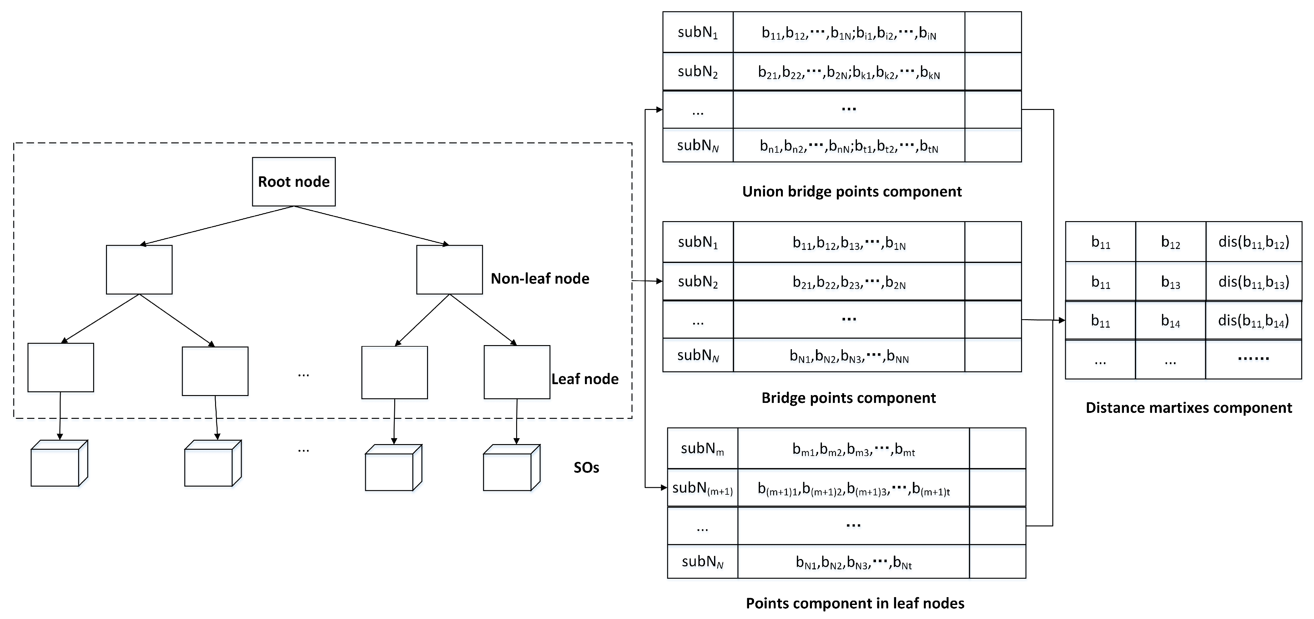
4.1. HN-Tree Index Definition

A key part of building the HN-tree is hierarchically partitioning the road network as described in Section 3. To support range queries, the HN-tree uses pre-computed distance matrices that are computed once the entire tree of partitions has been constructed.

Definition 6

(Distance matrix). Each leaf node maintains a distance matrix D that records the shortest path distance between bridge points and its network nodes. The distance matrix records the shortest path distances between all bridge points of its child nodes (union bridge points) in each non-leaf node. The distance matrices can be stored in the main memory or disk depending on the size of the network.

Note that unless otherwise stated in the paper, the distance is the network shortest path distance (SPDis) [19].

The HN-tree is a balanced index tree that has the following properties:

(1)

Each tree node captures a sub-network partition, the root node corresponds to the entire road network. The sub-network of the parent node is a super-network of its child nodes.

(2)

Each non-leaf node has at least $m(\ge$2) and at most M child nodes.

(3)

Each leaf node contains at most $\beta$ SOs. All leaf nodes appear at the same level.

(4)

Each tree node maintains bridge points and a distance matrix.

Figure 7 shows the HN-tree structure. Different types of tree nodes exist and respective information is captured for each. All non-leaf nodes including the root node can be described as $<B,U,D,child-pointer>$, where B is the set of its bridge points, U is the union set of all bridge points in child nodes, $child-pointer$ is a pointer to its child nodes, and D represents its distance matrix. The leaf node can be represented as $<B,D,tuple-identifier>$, the tuple-identifier is the set of SOs that a leaf node maintains, B is the set of corresponding bridge points, and D indicates its distance matrix. The HN-tree is a balanced indexing tree as all leaf nodes are on the same level.

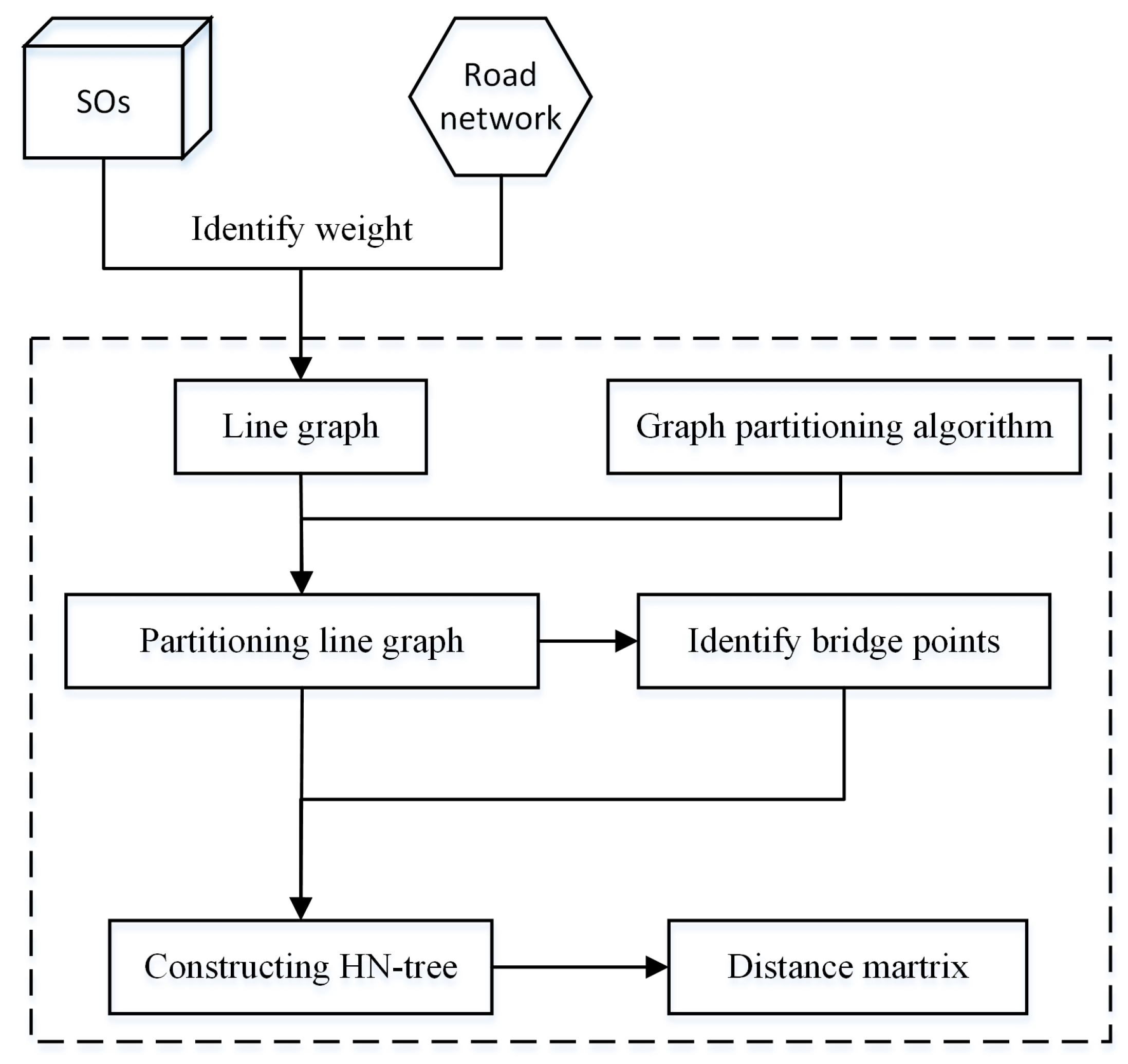
4.2. Index Construction

Based on the results of the hierarchical graph partitioning, the HN-tree with a root node, non-leaf nodes, and leaf nodes can be constructed. Initially, the root that is corresponding to a whole network G is a single leaf node. It does not contain any other tree nodes initially. Then, the sub-networks of G become the root’s child nodes. The root becomes a non-leaf node. Moreover, each subgraph corresponds to an HN-tree node and the relationships between tree nodes are equal to that of the sub-network. A sub-network without sub-networks is a leaf node. For each sub-network, bridge points are identified and added to the corresponding tree node. Moreover, the distance matrices should be computed, which is from leaf nodes to the root. The computing method of distance matrices is similar to [19]. Algorithm 1 presents the detail of the HN-tree construction process.

Algorithm 1. HN-tree construction

Require:$HP$: the results of the hierarchical graph partition; G: road network;

Ensure: HN-tree;

1: foreach $sub{\overline{G}}_i\in HP$ do

2:    convert $sub{\overline{G}}_i$ back to $sub{G}_i$

3: G is the root node of HN-tree;

4: the $sub{G}_i$ of G are corresponding to root node’s child nodes;

5: identify the bridge points of $sub{G}_i$;

6: while ($sub{G}_i$ is not the bottom partition) do

7:    add the next level’s $sub{G}_{i+1}$ of $sub{G}_i$ as its child nodes;

8:    identify the bridge points of $sub{G}_{i+1}$;

9: end while foreach tree node $tn\in$ HN-tree do

10:     compute the distance matrix of $tn$

11: return HN-tree;

5. Range Query Processing

Following the introduction of some key definitions, we introduce the range query algorithm and present distance computation functions.

To compute distances between network nodes in different partitions (and possibly on different levels of the HN-tree), the distance matrix D of a partition also includes distances between bridge points of the partition to bridge points of other adjacent partitions. We call such bridge points hierarchically adjacent points, defined as follows.

Definition 7

(Hierarchical adjacent points). Given a bridge point $v\in B\left(sub{G}_i\right)$ in partition $sub{G}_i$, other bridge points $\in B\left(sub{G}_i\right)$ are called hierarchically adjacent points. Since a bridge point(v) can be in several partitions at the same level, the union set of bridge points of these partitions is denoted as the set of hierarchically adjacent points $HAP\left(v\right)$ of v.

Hierarchical adjacent points of a bridge point at different levels can be extracted from the HN-tree when required by a query.

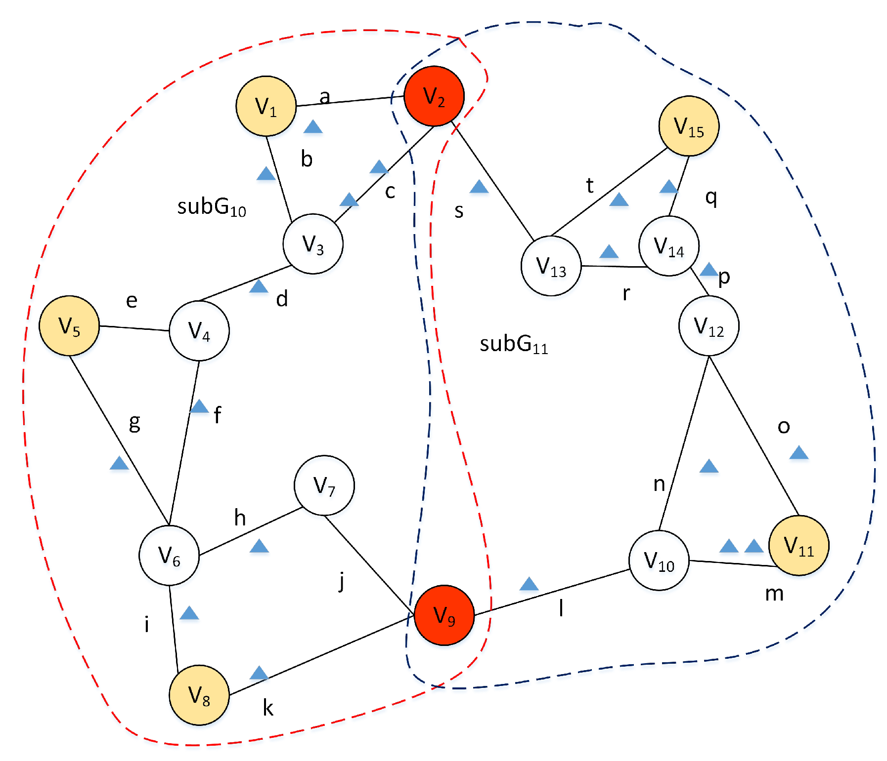
5.1. Concepts and Terminology

Some key definitions for our range query algorithm are as follows.

Definition 8

(Valid network node). Given a network G, a query point q, and range distance $d_r$, a network node $v\in G$ is valid if $SPDis(q,v)\le d_r$.

Definition 9

(Valid link/partially valid link/invalid link). Given a link $e_i$, a query point q, and range query distance $d_r$. If both nodes of link $e_i$ are valid, $e_i$ is called a valid link; if both nodes are invalid, $e_i$ is defined as a invalid link. Otherwise, $e_i$ is defined as a partially valid link.

Definition 10

(Valid partition/partially valid partition/invalid partition). Given a graph $sub{G}_i$, a query point q, and range query distance $d_r$, if the distances between $B\left(sub{G}_i\right)$ and q are less than $d_r$ ($SPDis(b_i,q)\le d_r$), $sub{G}_i$ is a valid partition. If the distances between $B\left(sub{G}_i\right)$ and q are greater than $d_r$, $sub{G}_i$ is an invalid partition. Besides, if q is in $sub{G}_i$, $sub{G}_i$ is a partially valid partition.

5.2. Range Query Algorithm

Given a query point q (on the road network) and a range distance $d_r$, we retrieve all valid nodes whose shortest path distance to $q\le d_r$. The algorithm consists of a filter and a refinement step. The filter step identifies qualifying leaf nodes. The refinement step then retrieves the actual valid SOs. Algorithm 2 shows the skeleton of our range query algorithm. The result sets $Res$ and refinement nodes set $P_{ref}$ are initially set to empty. The detailed process of the range query algorithm is as follows:

Filter step: (line 1–30): the algorithm first loads the whole tree. Beginning at the root node, the leaf node that contains q is located. Then, to compute the distances between leaf(q)’s bridge points and q, the validness of the leaf(q) is identified. If leaf(q) is invalid, the algorithm will insert leaf(q) in $EN$, and the refinement step starts. When leaf(q) is partially valid, the NNV function is used, which is a network partition expansion method that retrieves the tree nodes that potentially contain SOs within the query range. Algorithm 3 details the NNV function. Otherwise, the algorithm needs to compute the distances between the bridge points of its father node and q until the ancestor node is partially valid. Next, NNV is used. With $P_{ref}$ not empty, each leaf node in $P_{ref}$ is identified and inserted into $EN$. The algorithm will execute the refinement step. For all non-leaf nodes, the algorithm adds all child nodes to $EN$. When $EN$ is not empty, each tree node $tn\in EN$ is checked. A refinement step is executed for all $tn$ that are leaf nodes and the next element is identified. If $tn$ is a non-leaf node, the algorithm computes the distances between bridge points of its child nodes and q, and then identifies the validness of child nodes. If a child node is at least partially valid, the algorithm will insert it into $EN$. This process is repeated until the qualified leaf nodes are confirmed.

Refinement step: (line 31–41): the refinement step identifies all SOs in the database fulfilling the query criterion based on the approximate filter step results. Since SOs maintain the links’ ids and to improve the efficiency, each link is validated. Therefore, the algorithm will compute the distances between network nodes of each tree node in $EN$ and q. When the link’s id is valid, it will be added to $Res$. If it is partially valid, then, the algorithm will further compute the distance between the SOs and q and if less than $d_r$, SOs will be inserted into $Res$. Especially for a leaf node that contains the query point. If it is partially valid, INE [18] is used to compute the distances. If the SO does not meet the above demands, it is discarded.

Algorithm 2. Range query

Require:q: query point; $d_r$: a range distance; a HN-tree Ensure: Result set($Res$);       Local: refinement tree node set ($P_{ref}$), Effective tree nodes set ($EN$);       //Part 1: filter part   1: Initialize $P_{ref}=\varnothing ,Res=\varnothing ,EN=\varnothing$;   2: load HN-tree;   3: locate the leaf node that contains q;   4: foreach bridge point $b\in B\left(leaf\right(q\left)\right)$ do   5:     compute distance between b and q;   6: if$leaf\left(q\right)$ is partially invalid then   7:     $P_{ref}=NNV\left(leaf\left(q\right)\right)$;   8: else if $leaf\left(q\right)$ is invalid then   9:     $EN$.insert($leaf\left(q\right)$);   10:     goto Part 2;   11: else if$leaf\left(q\right)$ is valid then   12:     find the $leaf\left(q\right)$’s lowest ancestor node is partially valid ($TopTn\left(q\right)$);   13:     $P_{ref}=NNV(TopTn\left(q\right)$);   14: foreach tree node $tn\in P_{ref}$ do;   15:     if $tn$ is non-leaf node then   16:         foreach child node $ctn$ of $tn$ do   17:            compute the distance between $B\left(ctn\right)$ and q;   18:            if $ctn$ is partially valid or valid then   19:                $EN$.insert($ctn$);   20:         foreach tree node $tn\in EN$ do   21:            if $tn$ is leaf node then   22:                continue;   23:            else   24:                foreach child node $ctn$ of $tn$ do   25:                    compute the distance between $B\left(ctn\right)$ and q;   26:                    if $ctn$ is partially valid or valid then   27:                        $EN$.insert($ctn$);   28:                $EN$.erase($tn$);   29:     else   30:         $EN$.insert($tn$); //Part 2: refinement part   31: foreach leaf node $tn\in EN$ do   32:     foreach network node $v_i$ in $tn$ do   33:         compute the distance between $v_i$ and q;   34:     foreach link $e_i\in tn$ do   35:         if $e_i$ is valid then   36:            $Res$.insert($e_i$.SOs);   37:         else if $e_i$ is partially valid then   38:            foreach SO is on $e_i$ do   39:                if SPDis(SO, q)$\le d_r$ then   40:                    $Res$.insert(SO);   41: return$Res$;

Algorithm 3 presents the pseudo-code for the NNV function. The algorithm first inserts the bridge points of $TopTn$ into $PQb$, since the distances between $B\left(TopTn\right)$ and q are known. Moreover, the algorithm inserts $TopTn$ into $P_{ref}$. Next, while $PQb$ is not empty, the first element of $PQb$ that is marked as visited should be checked if its distance is less than $d_r$. The algorithm needs to compute the distances between nodes in $HAP\left(b\right)$ and q when the network node is not visited, and then the distances of $HAP\left(b\right)$ are updated to be inserted into $PQb$ if it satisfies the condition. The algorithm inserts the tree node that is at the same level as $TopTn$ containing the network node into $P_{ref}$ when it is not in $P_{ref}$. Since a bridge point can belong to two or more tree nodes, if the shortest path distance of a network node $HAP\left(b\right)$ with q has been identified, it does not need to be computed multiple times. The algorithm repeats this process until the first element’s distance is greater than $d_r$. Finally, the algorithm can find the qualified tree nodes at the level of $TopTn$.

Algorithm 3. Function NNV

Require:q: query point; $d_r$: a range distance; $TopTn$; Ensure: Refinement nodes set $P_{ref}$;   1: Initialize priority queue $PQb=\varnothing$, $P_{ref}=\varnothing$;   2: $P_{ref}$.enqueue($TopTn$)   3: foreach bridge point $b\in B\left(TopTn\right)$ do   4:     $PQb$.enqueue($b,SPDis(b,q)$);   5:     mark b visited;   6: while$PQb$ is not empty do   7:     $b\leftarrow PQb$.dequeue();   8:     mark b visited;   9:     if $SPDis(b,q)<d_r$ then   10:         find tree node $tn$ containing b; //$tn$ and $TopTn$ are at the same level   11:         if $tn$ is not in $P_{ref}$ then   12:            $P_{ref}$.enqueue($tn$)   13:         foreach $v\in HAP\left(b\right)$ do   14:            if v is visited then   15:                continue;   16:            else   17:                update $SPDis(v$, q);   18:                $PQb$.enqueue $(v,SPDis(v,q\left)\right)$;   19:     else   20:         break;   21: return$P_{ref}$

5.3. SPDis Function

One issue that remains with range queries is how to compute the shortest path distance(SPDis) between u and v. This is an essential function for the HN-tree, since it will directly affect the range query performance.

SPDis($\mathbf{u}$,$\mathbf{v}$) in the same leaf: given two network nodes v and u we compute the shortest path distance SPDis(v,u) using the Dijkstra algorithm. The Dijkstra algorithm in this case is efficient since the size of a leaf node is small.

SPDis($\mathbf{u}$,$\mathbf{v}$) in different leaf nodes: given two network nodes v and u in two different leaf nodes, we use a dynamic programming algorithm to calculate SPDis(u,v). The main idea is as follows: let LCA(u,v) represent the lowest common ancestor of nodes $leaf\left(v\right)$ and $leaf\left(u\right)$, i.e., the respective leaf nodes containing v and u.

Given the tree nodes on a path for LCA (u,v), then all bridge points are combined to get the shortest path distance. For the more details, see [19].

6. Experimental Evaluation

In this section, we compare the HN-tree index and related query performance to a range of competitor approaches using different road networks, spatial object datasets, and query sizes.

6.1. Datasets

Available datasets are not sufficiently representative in terms of the distribution of SOs and data size. Therefore, we use the data generator for SOs proposed in [42] to generate synthetic datasets. This so-called Brinkhoff generator is available with several networks and we use three of them: the road networks for the cities of (i) Oldenburg (Germany), (ii) San Joaquin (US), and (iii) San Francisco Bay Area (U.S.). The network is represented in a link-oriented model, i.e., each link represents a road and has a unique identifier. Oldenburg has 6105 network nodes and 7034 links, San Joaquin has 18,496 network nodes and 24,123 links, and the San Francisco Bay Area has 175,343 network nodes and 223,606 links. Concerning the number of SOs for different networks, Oldenburg has 1,248,212 SOs, San Joaquin has 3,305,742 SOs, and the Francisco Bay Area has 37,808,266 SOs. Moreover, these SO datasets follow a non-uniform distribution in the network.

Table 1. Dataset characteristics.

Name	# of Network Nodes	# of Links	# of SOs
Oldenburg	6105	7034	1,248,212
San Joaquin	18,496	24,123	3,305,742
San Francisco Bay Area	175,343	223,606	37,808,266

summarizes the characteristics of the three datasets.

6.2. Experimental Setup

To analyze the performance of the HN-tree, we implement and compare several spatial indexing schemes using the same basic experimental framework.

Experimental environment: all experiments are implemented in C++ and run on an Intel i7, 2.6 GHz CPU, 16 GB RAM, and Windows 64-bit operating system.

Approaches compared: to better evaluate the performance of the HN-tree, we design two baseline indexing methods, Flat A and Flat B. Those methods use the same number of partitions.

Flat A: partitions the road network into equally sized partitions with an equal number of links based on METIS. Its indexing structure is the same as VRS [17], and we only discard the adjacent components portion.

Flat B: partitions the SOs into equal sized partitions. The same indexing structure and query process algorithm as for Flat A.

Voronoi-based range search (VRS) [17] and G*-tree [28]: state-of-the-art algorithm.

We note that we cannot compare directly the G-tree [19] since it only considers the case of having nodes as possible spatial objects locations. It cannot be used directly for our case where spatial objects may be located on edges, as edges are lost in the partitioning. While it is possible to transform a network having spatial objects on edges into a network having all spatial objects on nodes by adding pseudo nodes (potentially one pseudo-node per spatial objects), this is not feasible due to our large number of spatial objects in our datasets (see Table 1). In addition, the G-tree only supports KNN queries. Using its KNN algorithm to implement a range query algorithm will result in poor performance. If the object density (the number of objects relative to the number of vertexes) is >1, the performance is much worse than INE [18] as shown in the G-tree experimentation [19]. However, VRS [17] always outperforms INE for range queries, and thus we choose VRS as a competitor.

Instead, we compare to the G*-tree [28], which supports range queries, but also assumes that spatial objects are located on the nodes of the road network. For comparison, we map each spatial object to the nearest network node for G*-tree experiments.

Performance metrics: we use four performance metrics: (i) construction time; (ii) query time; (iii) the number of computed network nodes (number of shortest paths computations that are needed to process a query); and (iv) the number of refined spatial objects.

6.3. Dataset: Non-Uniform Distribution

Query sizes are 0.1%, 0.5%, 1%, 2.5%, 5%, and 10% of the total length of links in the network. The query points are randomly selected based on SOs, and then we perform 20 queries for different query sizes. We calculate average values for each query. For HN-tree, considering the query performance, construction time, and space overhead, after a lot of testing, the default fan-out is 8.

Index construction time: the first experiment evaluates the index construction time for all approaches and different datasets. Note that the construction times of HN-tree, G*-tree Flat A, and Flat B includes graph partitioning, tree construction, and computing the distance matrices. However, since VRS uses SANET to generate the Voronoi units and identify the border points, its construction time only covers computing distance matrices. Figure 8 shows the index construction times. We can observe that all methods take more time to construct indexes for larger road networks. Moreover, VRS always outperforms the other approaches. HN-tree, G*-tree, Flat A, and Flat B utilize METIS to partition the road network. However, only HN-tree, Flat A, and Flat B use a line graph to identify the bridge points of each tree node. These steps take extra time. G*-tree directly partitions the road network graph. These four indexes have similar construction times.

Query Time: the results are shown in Figure 9. The vertical axis represents running time (in ms), while the horizontal axis shows the query size. We can observe that the HN-tree always outperforms the other three methods for different datasets and query sizes. Query times increase with network size. VRS outperforms G*-tree, Flat A, and Flat B. Flat B slightly outperforms Flat A.

Number of computed network nodes: it is an important metric since it affects query time. The HN-tree consistently outperforms all other methods as shown in Figure 10. Since Flat A and Flat B compute bridge points for all partitions, they are far more than for VRS and the HN-tree. The HN-tree needs fewer computed network nodes than VRS and G*-tree, especially for small range queries. In addition, we can also find that query time is proportional to the number of computed network nodes.

The number of refinements: the results of this often overlooked metric are shown in Figure 11. The HN-tree outperforms all other methods. When a query point is in a high density area, the HN-tree needs to retrieve fewer actual SOs in the refinement step given its smaller search area. Flat A, VRS, and G*-tree show similar results, since they all only rely on the topology to partition the road network (and not the data).

6.4. Datasets: Different Distributions

To further assess the performance of the HN-tree for different data distributions, we perform experiments on a dataset with a uniform distribution and a mixed distribution. Therefore, we use the “Brinkhoff” generator to create a dataset with 2,941,805 SOs that places SOs uniformly on the San Joaquin network. Following a uniform distribution, the number of objects is proportional to the length of a link. A mixture dataset is obtained by taking the various percentages of non-uniform (previous experiment) vs. uniform data. The percentages of the uniform data in the six datasets are 0%, 10%, 25%, 50%, 75%, 90%, and 100%, respectively.

Figure 12 shows the results for the mixed dataset with a 1% query size. We choose the query points based on SOs. The query times are increasing with an increasing portion of uniform data for the case of the HN-tree.

Compared to VRS, the query times and computed nodes advantage of the HN-tree is reduced with an increasing percentage of uniform data. Moreover, when the percentage reaches 75% and 100%, the query time of HN-tree still slightly outperforms VRS. HN-tree always outperforms the G*-tree for the query times and computed nodes. For the number of refined spatial objects, the advantage of the HN-tree gradually diminishes when with an increasing uniform data percentage.

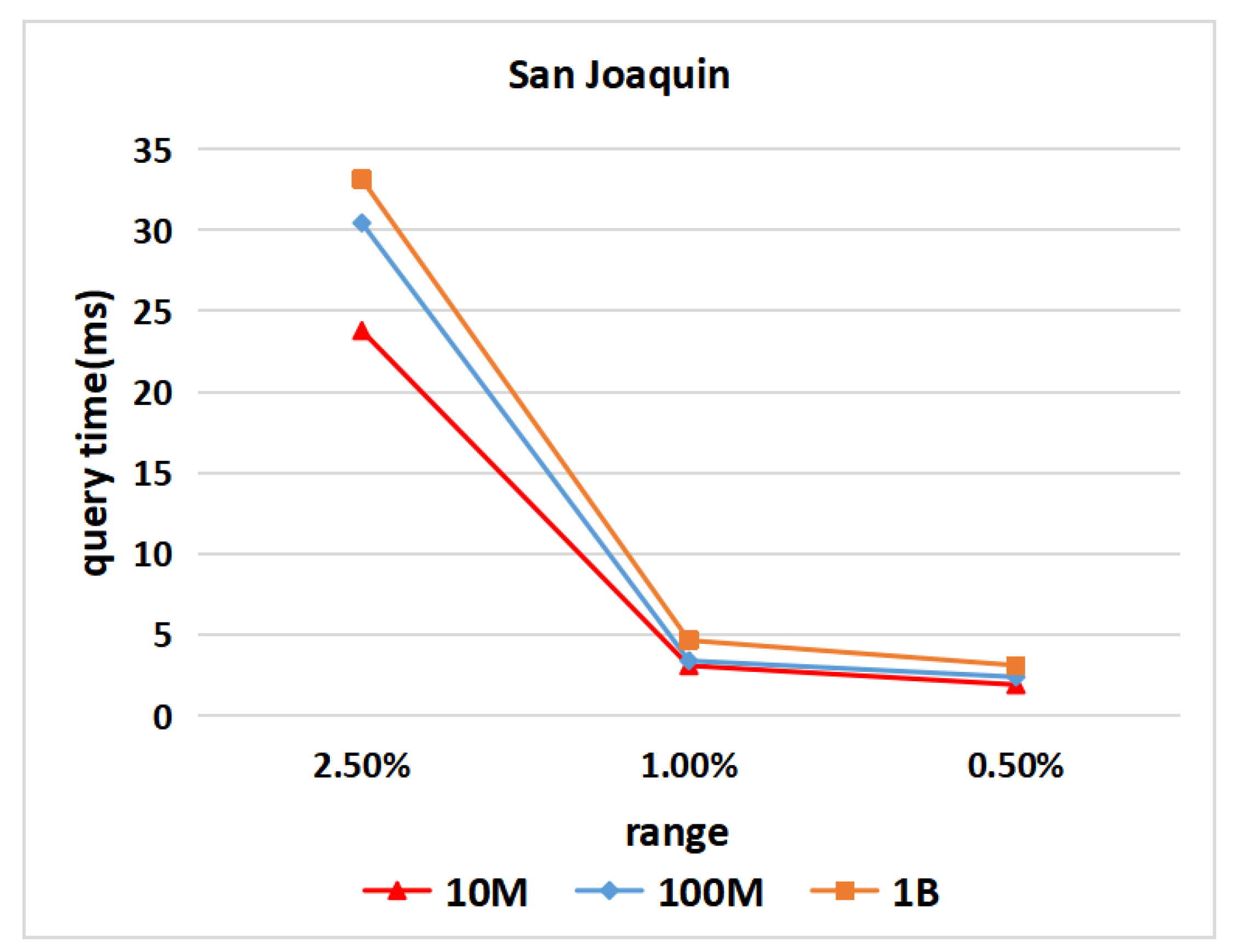
6.5. Query Time for Different Numbers of Spatial Objects

To understand how range queries, supported by our HN-tree, scale as the number of spatial objects increases, we next perform experiments where we scale up the number of spatial objects while keeping the size of the underlying spatial network and the query range constant. Using the spatial network of San Joaquin (which normally has 3,305,742 spatial objects), we generate 10 M(million), 100 M, and 1 B(billion) spatial objects on this network having locations distributed uniformly across the spatial network.

Figure 13 presents the results of this experiment using query sizes of 2.5%, 1%, and 0.5%. We observe that the query time increase sublinear in the number of spatial objects. For example, using a 1% range query the query time increases from 3 ms to 5 ms as we scale the number of spatial objects from 10 M to 1 B. The reason for this sublinear scaling is that, while the number of spatial objects to be returned increases linear in the number of spatial objects (since the query range and underlying network are held constant), the network that needs to be explored by Algorithm 2 decreases, since more spatial objects implies more leaf partitions which cover less space outsize of the query range. This exploration of the spatial network is the main computational bottleneck; thus, we observe a sublinear increase in run-time.

6.6. Experimentation Summary

Our evaluation mainly focuses on testing the performance of the HN-tree relative to the baseline methods, such as Flat A, Flat B, and VRS and G*-tree. The results show that the HN-tree is the most efficient method to support range queries. The HN-tree ensures that each partition has a similar number of SOs since it uses a data and space driven hierarchical partitioning method. This performance advantage persists for different query sizes and datasets. Hence, the experimental results show the considerable robustness and practicality of the HN-tree. Regarding memory consumption, the main memory bottleneck of the HN-tree is storing the distance matrices. We note that in all our experiments the memory consumption of these matrices is less than the space overhead of road network and spatial objects.

7. Conclusions and Future Work

This work proposes a novel access method named HN-tree in support of efficient range query processing of spatial objects on road networks. We use METIS, a heuristics-based multilevel k-way graph partitioning algorithm to partition the road network, and then to construct a hierarchical network indexing tree. As part of the partitioning process, we generate a so-called line graph, which is a transformation of the road network graph that models edges and numbers of spatial objects as vertices and corresponding weights. The line graph is decomposed recursively until each partition contains a max number of spatial objects (represented as node weights in the line graph). The resulting set of hierarchical partitions is used to construct the HN-tree. The HN-tree performance is assessed by comparing its performance to (i) two baseline and two state-of-the-art indexing methods; (ii) using three different road networks; and (iii) varying query sizes. The results suggest that the HN-tree performance is superior to its competitor methods in terms of query time, the number of computing network nodes, and the number of refinements. The good performance of the HN-tree for uniform and mixed distributions of data further illustrates the advantage of this novel method. Therefore, HN-tree has an important advantage over the existing methods, since HN-tree can be adaptive to different distribution types of SOs on the road network to get better performance.

Directions for future work include (i) improving the quality of the hierarchical graph partitioning and reducing the construction time; (ii) a dynamic indexing schema for updating and deleting data from our index; (iii) an access method that supports online indexing and can handle streaming data; and (iv) solutions for approximate range query processing.

References

1. Li, S.; Dragicevic, S.; Castro, F.A.; Sester, M.; Winter, S.; Coltekin, A.; Pettit, C.; Jiang, B.; Haworth, J.; Stein, A.; et al. Geospatial big data handling theory and methods: A review and research challenges. ISPRS J. Photogramm. Remote Sens. 2016, 115, 119–133. [Google Scholar] [CrossRef] [Green Version]
2. Shekhar, S.; Chawla, S.; Ravada, S.; Fetterer, A.; Liu, X.; Lu, C.T. Spatial databases-accomplishments and research needs. IEEE Trans. Knowl. Data Eng. 1999, 11, 45–55. [Google Scholar] [CrossRef]
3. Tong, Y.; Zhou, Z.; Zeng, Y.; Chen, L.; Shahabi, C. Spatial crowdsourcing: A survey. VLDB J. 2020, 29, 217–250. [Google Scholar] [CrossRef]
4. Yan, Y.; Feng, C.C.; Huang, W.; Fan, H.; Wang, Y.C.; Zipf, A. Volunteered geographic information research in the first decade: A narrative review of selected journal articles in GIScience. Int. J. Geogr. Inf. Sci. 2020, 34, 1765–1791. [Google Scholar] [CrossRef]
5. Lin, J.; Wu, Z.; Li, X. Measuring inter-city connectivity in an urban agglomeration based on multi-source data. Int. J. Geogr. Inf. Sci. 2019, 33, 1062–1081. [Google Scholar] [CrossRef]
6. Ester, M.; Kriegel, H.P.; Sander, J.; Xu, X. A density-based algorithm for discovering clusters in large spatial databases with noise. KDD-96 Proc. 1996, 96, 226–231. [Google Scholar]
7. Guttman, A. R-trees: A dynamic index structure for spatial searching. In Proceedings of the 1984 ACM SIGMOD International Conference on Management of Data, Boston, MA, USA, 18–21 June 1984; pp. 47–57. [Google Scholar]
8. Sun, W.; Chen, C.; Zheng, B.; Chen, C.; Liu, P. An air index for spatial query processing in road networks. IEEE Trans. Knowl. Data Eng. 2014, 27, 382–395. [Google Scholar] [CrossRef]
9. Hoffman, J. Q&A: The data visualizer. Nature 2012, 486, 33. [Google Scholar]
10. Pfoser, D.; Jensen, C.S.; Theodoridis, Y. Novel approaches to the indexing of moving object trajectories. In Proceedings of the 26th VLDB Conference, Cairo, Egypt, 10–14 September 2000. [Google Scholar]
11. Cudre-Mauroux, P.; Wu, E.; Madden, S. Trajstore: An adaptive storage system for very large trajectory data sets. In Proceedings of the 2010 IEEE 26th International Conference on Data Engineering (ICDE 2010), Long Beach, CA, USA, 1–6 March 2010; pp. 109–120. [Google Scholar]
12. Al Aghbari, Z. cTraj: Efficient indexing and searching of sequences containing multiple moving objects. J. Intell. Inf. Syst. 2012, 39, 1–28. [Google Scholar] [CrossRef]
13. Song, M.; Choo, H.; Kim, W. Spatial indexing for massively update intensive applications. Inf. Sci. 2012, 203, 1–23. [Google Scholar] [CrossRef]
14. Gani, A.; Siddiqa, A.; Shamshirband, S.; Hanum, F. A survey on indexing techniques for big data: Taxonomy and performance evaluation. Knowl. Inf. Syst. 2016, 46, 241–284. [Google Scholar] [CrossRef]
15. Pfoser, D.; Jensen, C.S. Trajectory indexing using movement constraints. GeoInformatica 2005, 9, 93–115. [Google Scholar] [CrossRef] [Green Version]
16. Popa, I.S.; Zeitouni, K.; Oria, V.; Barth, D.; Vial, S. Indexing in-network trajectory flows. VLDB J. 2011, 20, 643. [Google Scholar] [CrossRef]
17. Xuan, K.; Zhao, G.; Taniar, D.; Rahayu, W.; Safar, M.; Srinivasan, B. Voronoi-based range and continuous range query processing in mobile databases. J. Comput. Syst. Sci. 2011, 77, 637–651. [Google Scholar] [CrossRef] [Green Version]
18. Papadias, D.; Zhang, J.; Mamoulis, N.; Tao, Y. Query processing in spatial network databases. In Proceedings 2003 VLDB Conference; Elsevier: Amsterdam, The Netherlands, 2003; pp. 802–813. [Google Scholar]
19. Zhong, R.; Li, G.; Tan, K.L.; Zhou, L.; Gong, Z. G-tree: An efficient and scalable index for spatial search on road networks. IEEE Trans. Knowl. Data Eng. 2015, 27, 2175–2189. [Google Scholar] [CrossRef]
20. Lee, K.C.; Lee, W.C.; Zheng, B.; Tian, Y. ROAD: A new spatial object search framework for road networks. IEEE Trans. Knowl. Data Eng. 2010, 24, 547–560. [Google Scholar] [CrossRef]
21. Chen, L.; Tang, Y.; Lv, M.; Chen, G. Partition-based range query for uncertain trajectories in road networks. GeoInformatica 2015, 19, 61–84. [Google Scholar] [CrossRef]
22. Teng, X.; Yang, J.; Kim, J.S.; Trajcevski, G.; Züfle, A.; Nascimento, M.A. Fine-grained diversification of proximity constrained queries on road networks. In Proceedings of the 16th International Symposium on Spatial and Temporal Databases, Vienna, Austria, 19–21 August 2019; pp. 51–60. [Google Scholar]
23. Pfoser, D. Indexing the trajectories of moving objects. IEEE Data Eng. Bull. 2002, 25, 3–9. [Google Scholar]
24. Bentley, J.L. Multidimensional binary search trees in database applications. IEEE Trans. Softw. Eng. 1979, 4, 333–340. [Google Scholar] [CrossRef]
25. Beckmann, N.; Kriegel, H.P.; Schneider, R.; Seeger, B. The R*-tree: An efficient and robust access method for points and rectangles. In Proceedings of the 1990 ACM SIGMOD International Conference on Management of Data, Atlantic City, NJ, USA, 23–25 May 1990; pp. 322–331. [Google Scholar]
26. Šumák, M.; Gurskỳ, P. R++-tree: An efficient spatial access method for highly redundant point data. In New Trends in Databases and Information Systems; Springer: Berlin/Heidelberg, Germany, 2014; pp. 37–44. [Google Scholar]
27. Xu, J.; Güting, R.H.; Zheng, Y. The TM-RTree: An index on generic moving objects for range queries. GeoInformatica 2015, 19, 487–524. [Google Scholar] [CrossRef]
28. Li, Z.; Chen, L.; Wang, Y. G*-Tree: An Efficient Spatial Index on Road Networks. In Proceedings of the 2019 IEEE 35th International Conference on Data Engineering (ICDE), Macao, China, 8–11 April 2019. [Google Scholar]
29. Zhang, H.; Lu, F.; Chen, J. A line graph-based continuous range query method for moving objects in networks. ISPRS Int. J. Geo-Inf. 2016, 5, 246. [Google Scholar] [CrossRef] [Green Version]
30. Yin, X.; Ding, Z.; Li, J. Moving continuous k nearest neighbor queries in spatial network databases. In Proceedings of the 2009 WRI World Congress on Computer Science and Information Engineering, Washington, DC, USA, 31 March–2 April 2009; Volume 4, pp. 535–541. [Google Scholar]
31. Jossé, G.; Schmid, K.A.; Züfle, A.; Skoumas, G.; Schubert, M.; Renz, M.; Pfoser, D.; Nascimento, M.A. Knowledge extraction from crowdsourced data for the enrichment of road networks. Geoinformatica 2017, 21, 763–795. [Google Scholar] [CrossRef]
32. Skoumas, G.; Schmid, K.A.; Jossé, G.; Schubert, M.; Nascimento, M.A.; Züfle, A.; Renz, M.; Pfoser, D. Knowledge-enriched route computation. In International Symposium on Spatial and Temporal Databases; Springer: Berlin/Heidelberg, Germany, 2015; pp. 157–176. [Google Scholar]
33. Wang, H.; Zimmermann, R. Processing of continuous location-based range queries on moving objects in road networks. IEEE Trans. Knowl. Data Eng. 2010, 23, 1065–1078. [Google Scholar] [CrossRef]
34. Lee, K.C.; Lee, W.C.; Zheng, B. Fast object search on road networks. In Proceedings of the 12th International Conference on Extending Database Technology: Advances in Database Technology, Saint Petersburg, Russia, 24–26 March 2009; pp. 1018–1029. [Google Scholar]
35. Frentzos, E. Indexing objects moving on fixed networks. In International Symposium on Spatial and Temporal Databases; Springer: Berlin/Heidelberg, Germany, 2003; pp. 289–305. [Google Scholar]
36. Dijkstra, E.W. A note on two problems in connexion with graphs. Numer. Math. 1959, 1, 269–271. [Google Scholar] [CrossRef] [Green Version]
37. Karypis, G.; Kumar, V. A fast and high quality multilevel scheme for partitioning irregular graphs. SIAM J. Sci. Comput. 1998, 20, 359–392. [Google Scholar] [CrossRef]
38. Anwar, T.; Liu, C.; Vu, H.L.; Leckie, C. Partitioning road networks using density peak graphs: Efficiency vs. accuracy. Inf. Syst. 2017, 64, 22–40. [Google Scholar] [CrossRef]
39. Hosseini, S.; Najafipour, S.; Cheung, N.M.; Yin, H.; Kangavari, M.R.; Zhou, X. TEAGS: Time-aware text embedding approach to generate subgraphs. Data Min. Knowl. Discov. 2020, 34, 1136–1174. [Google Scholar] [CrossRef]
40. Najafipour, S.; Hosseini, S.; Hua, W.; Kangavari, M.R.; Zhou, X. SoulMate: Short-text author linking through Multi-aspect temporal-textual embedding. IEEE Trans. Knowl. Data Eng. 2020. [Google Scholar] [CrossRef] [Green Version]
41. Ashrafi-Payaman, N.; Kangavari, M.R.; Hosseini, S.; Fander, A.M. GS4: Graph stream summarization based on both the structure and semantics. J. Supercomput. 2021, 77, 2713–2733. [Google Scholar] [CrossRef]
42. Brinkhoff, T. A Framework for Generating Network-Based Moving Objects. Geoinformatica 2002, 6, 153–180. [Google Scholar] [CrossRef]
Figure 1. The main process of graph partition.
Ijgi 10 00814 g001
Figure 2. Example of the two representations of a network. (a) geometric representation; (b) line graph.
Ijgi 10 00814 g002
Figure 3. Example of the four phases of hierarchical graph partitioning. (a) The first level of graph partitioning; (b) the second level of graph partitioning; (c) the third level of graph partitioning; (d) the fourth level of graph partitioning.
Ijgi 10 00814 g003
Figure 4. The example of road network partition.
Ijgi 10 00814 g004
Figure 5. Hierarchical graph partition results. (a) level 0; (b) level 1; (c) level 2.
Ijgi 10 00814 g005
Figure 6. HN-tree construction and query processing flowchart.
Ijgi 10 00814 g006
Figure 7. HN-tree structure.
Ijgi 10 00814 g007
Figure 8. Index construction time.
Ijgi 10 00814 g008
Figure 9. Query time (ms). (a) Oldenburg; (b) San Joaquin; (c) San Francisco.
Ijgi 10 00814 g009
Figure 10. Number of computed network nodes. (a) Oldenburg; (b) San Joaquin; (c) San Francisco.
Ijgi 10 00814 g010
Figure 11. Number of refinements. (a) Oldenburg; (b) San Joaquin; (c) San Francisco.
Ijgi 10 00814 g011
Figure 12. Mixed distribution of datasets query performance. (a) Query time (ms); (b) Number of computed network nodes; (c) Number of refinements.
Ijgi 10 00814 g012
Figure 13. Query time for different numbers of SOs.
Ijgi 10 00814 g013