
Instance Segmentation for Governmental Inspection of Small Touristic Infrastructure in Beach Zones Using Multispectral High-Resolution WorldView-3 Imagery

 ,
,  ,
,  , ,
, ,  , , , and
Abstract
:1. Introduction
2. Materials and Methods
2.1. Dataset
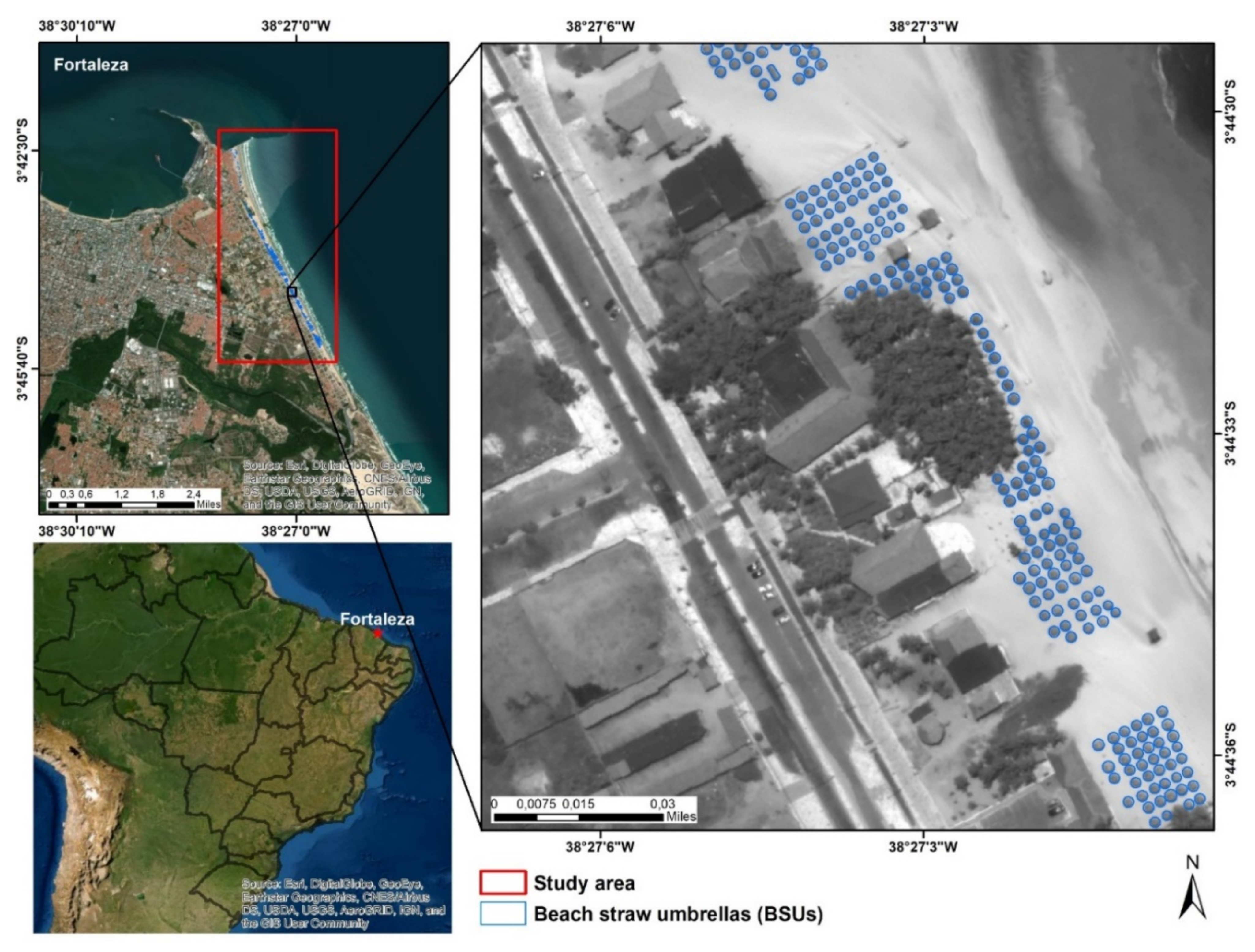
2.1.1. Study Area
2.1.2. Annotations
2.1.3. Clipping Tiles and Scaling
2.1.4. Data Split
2.2. Instance Segmentation Approach
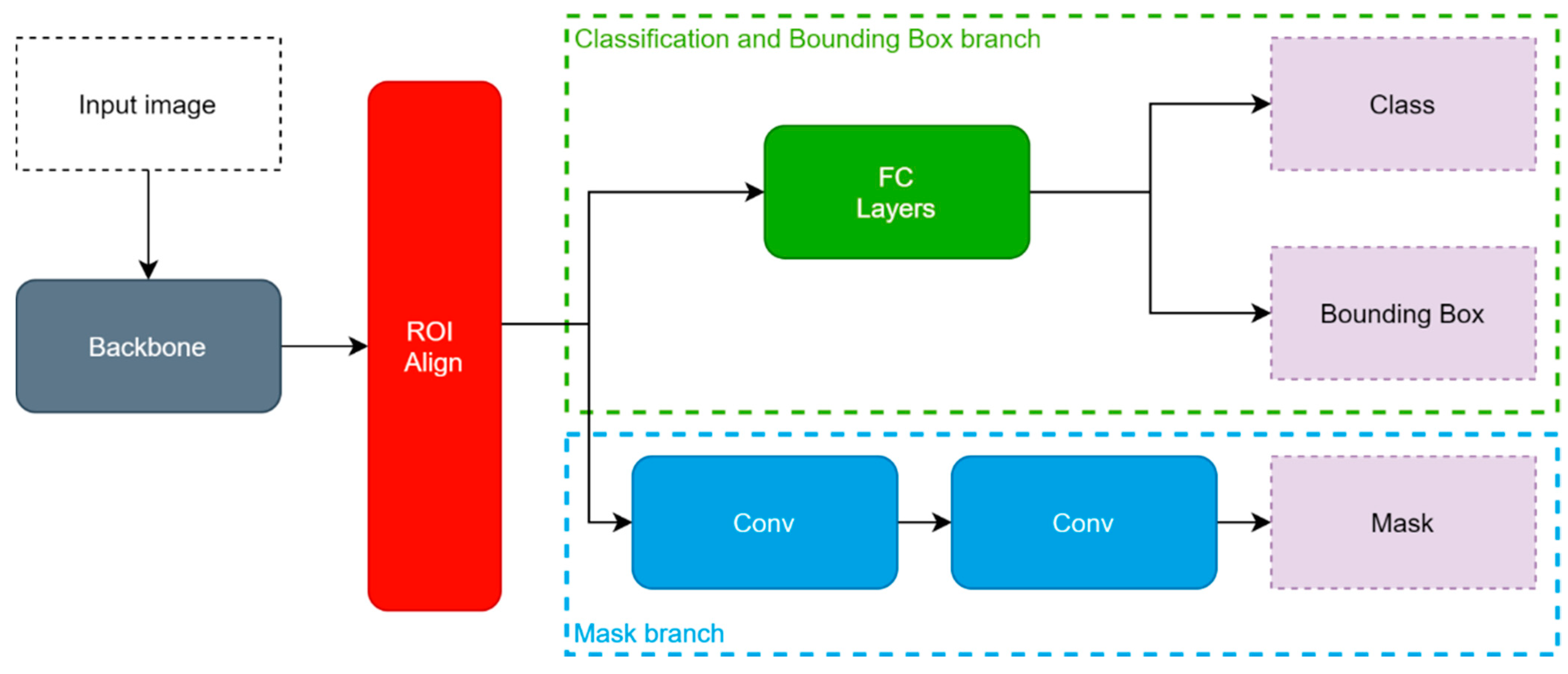
2.2.1. Mask-RCNN Architecture
2.2.2. Model Configurations
2.3. Image Mosaicking Using Sliding Windows
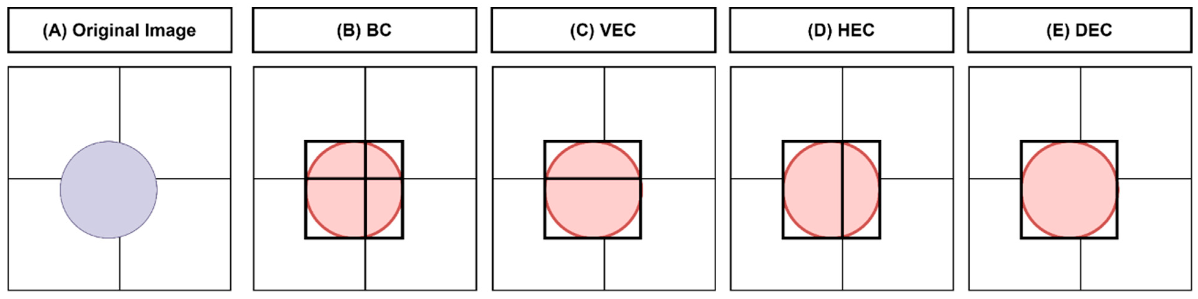
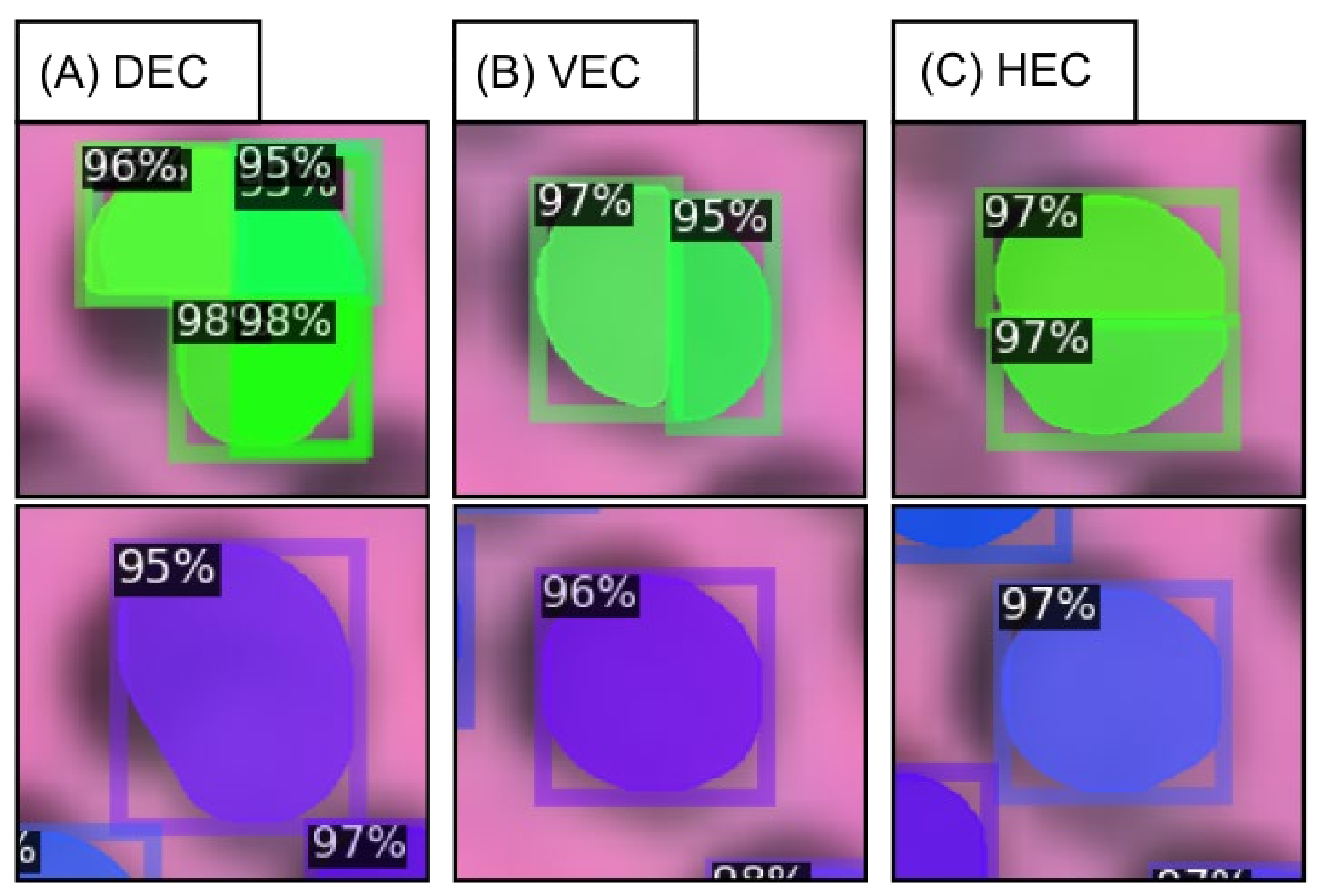
2.3.1. Base Classification
2.3.2. Single Edge Classification
2.3.3. Double Edge Classifier
2.3.4. Non-Maximum Suppression Sorted by Area
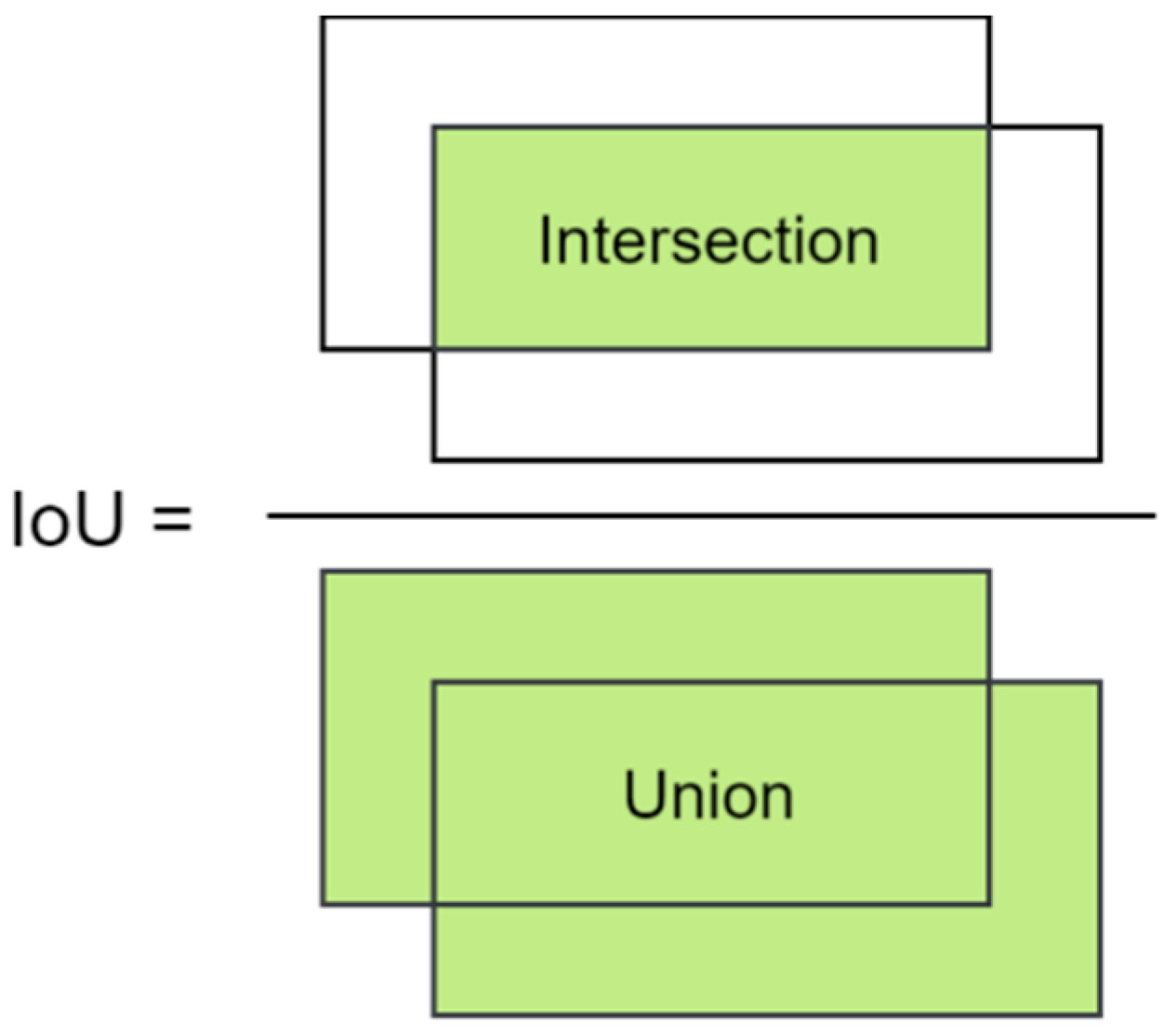
2.4. Performance Metrics
3. Results
3.1. Performance Metrics
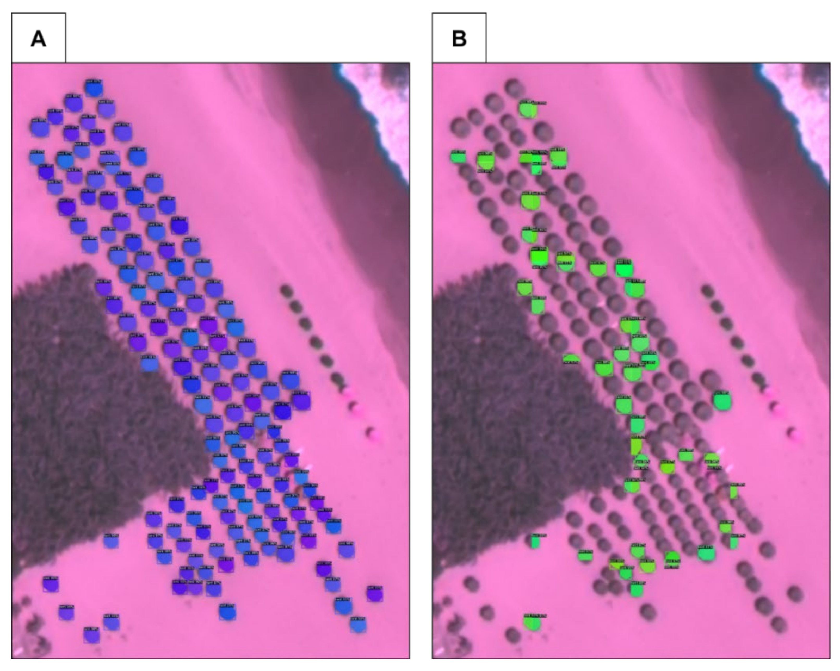
3.2. Scene Classification
4. Discussion
4.1. Multichannel Instance Segmentation Studies
4.2. Methods for Large Area Classification
4.3. Small Object Problem
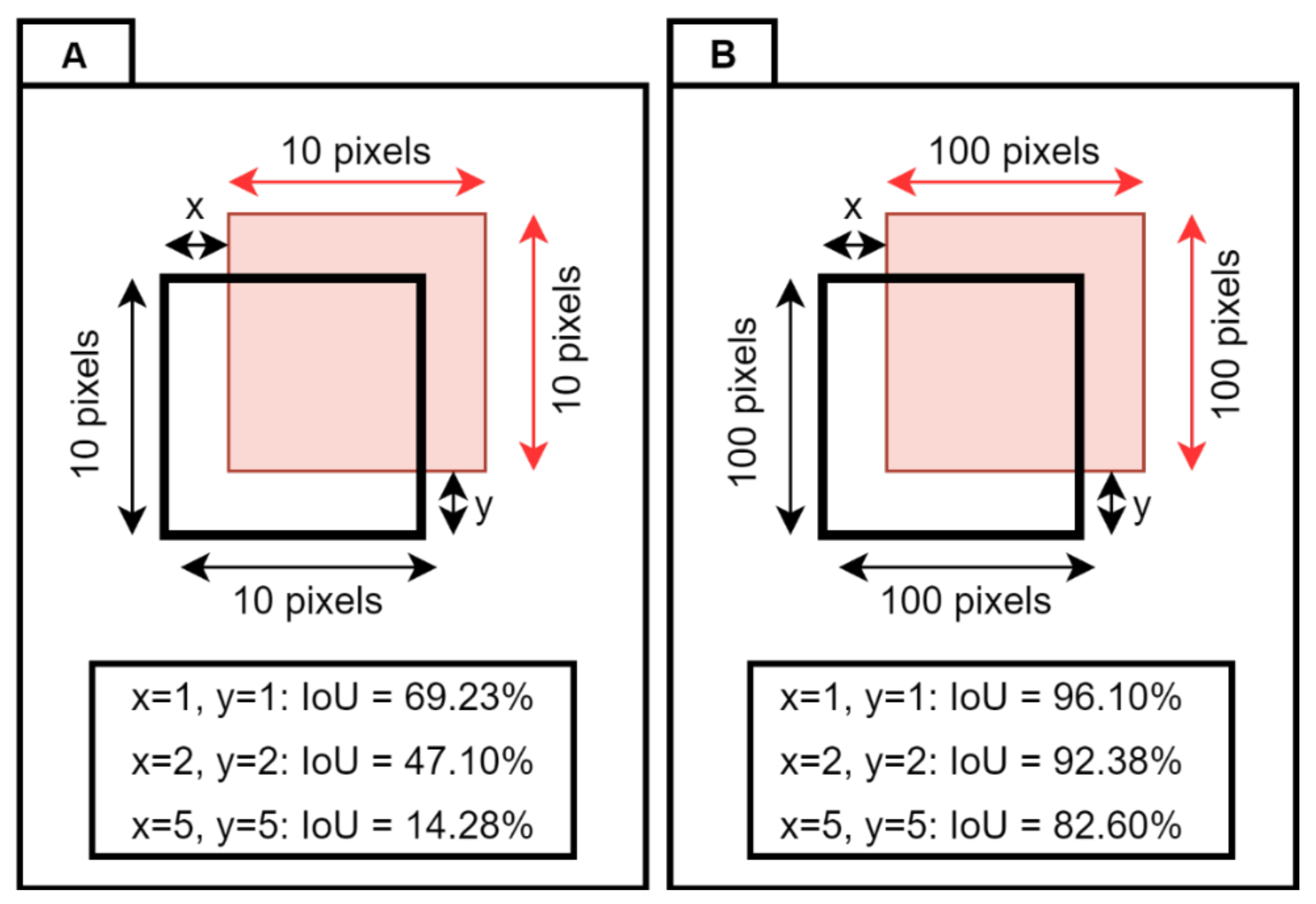
4.4. Accuracy Metric Analysis for Small Objects
4.5. Policy Implications
5. Conclusions
Author Contributions
Funding
Data Availability Statement
Acknowledgments
Conflicts of Interest
References
- Brown, G.; Weber, D.; de Bie, K. Assessing the value of public lands using public participation GIS (PPGIS) and social landscape metrics. Appl. Geogr. 2014, 53, 77–89. [Google Scholar] [CrossRef]
- DeFries, R.; Hansen, A.; Turner, B.L.; Reid, R.; Liu, J. Land use change around protected areas: Management to balance human needs and ecological function. Ecol. Appl. 2007, 17, 1031–1038. [Google Scholar] [CrossRef] [PubMed]
- Belal, A.A.; Moghanm, F.S. Detecting urban growth using remote sensing and GIS techniques in Al Gharbiya governorate, Egypt. Egypt. J. Remote Sens. Space Sci. 2011, 14, 73–79. [Google Scholar] [CrossRef] [Green Version]
- Dacey, S.; Song, L.; Pang, S. An intelligent agent based land encroachment detection approach. In Proceedings of the International Conference on Neural Information Processing, Daegu, Korea, 3–7 November 2013; pp. 585–592. [Google Scholar]
- Brown, G.; de Bie, K.; Weber, D. Identifying public land stakeholder perspectives for implementing place-based land management. Landsc. Urban Plan. 2015, 139, 1–15. [Google Scholar] [CrossRef]
- Martin, C.; Parkes, S.; Zhang, Q.; Zhang, X.; McCabe, M.F.; Duarte, C.M. Use of unmanned aerial vehicles for efficient beach litter monitoring. Mar. Pollut. Bull. 2018, 131, 662–673. [Google Scholar] [CrossRef] [PubMed] [Green Version]
- Serra-Gonçalves, C.; Lavers, J.L.; Bond, A.L. Global review of beach debris monitoring and future recommendations. Environ. Sci. Technol. 2019, 53, 12158–12167. [Google Scholar] [CrossRef]
- Gladstone, W.; Curley, B.; Shokri, M.R. Environmental impacts of tourism in the Gulf and the Red Sea. Mar. Pollut. Bull. 2013, 72, 375–388. [Google Scholar] [CrossRef]
- Burak, S.; Dogˇan, E.; Gaziogˇlu, C. Impact of urbanization and tourism on coastal environment. Ocean Coast. Manag. 2004, 47, 515–527. [Google Scholar] [CrossRef]
- He, Y.; Ma, W.; Ma, Z.; Fu, W.; Chen, C.; Yang, C.-F.; Liu, Z. Using Unmanned Aerial Vehicle Remote Sensing and a Monitoring Information System to Enhance the Management of Unauthorized Structures. Appl. Sci. 2019, 9, 4954. [Google Scholar] [CrossRef] [Green Version]
- Varol, B.; Yılmaz, E.Ö.; Maktav, D.; Bayburt, S.; Gürdal, S. Detection of illegal constructions in urban cities: Comparing LIDAR data and stereo KOMPSAT-3 images with development plans. Eur. J. Remote Sens. 2019, 52, 335–344. [Google Scholar] [CrossRef] [Green Version]
- Lira, C.; Taborda, R. Advances in Applied Remote Sensing to Coastal Environments Using Free Satellite Imagery. In Remote Sensing and Modeling; Finkl, C., Makowski, C., Eds.; Springer: Cham, Switzerland, 2014; pp. 77–102. [Google Scholar]
- Parthasarathy, K.S.S.; Deka, P.C. Remote sensing and GIS application in assessment of coastal vulnerability and shoreline changes: A review. ISH J. Hydraul. Eng. 2019, 1–13. [Google Scholar] [CrossRef]
- McCarthy, M.J.; Colna, K.E.; El-Mezayen, M.M.; Laureano-Rosario, A.E.; Méndez-Lázaro, P.; Otis, D.B.; Toro-Farmer, G.; Vega-Rodriguez, M.; Muller-Karger, F.E. Satellite Remote Sensing for Coastal Management: A Review of Successful Applications. Environ. Manag. 2017, 60, 323–339. [Google Scholar] [CrossRef]
- El Mahrad, B.; Newton, A.; Icely, J.; Kacimi, I.; Abalansa, S.; Snoussi, M. Contribution of Remote Sensing Technologies to a Holistic Coastal and Marine Environmental Management Framework: A Review. Remote Sens. 2020, 12, 2313. [Google Scholar] [CrossRef]
- Ouellette, W.; Getinet, W. Remote sensing for Marine Spatial Planning and Integrated Coastal Areas Management: Achievements, challenges, opportunities and future prospects. Remote Sens. Appl. Soc. Environ. 2016, 4, 138–157. [Google Scholar] [CrossRef]
- Ibarra-Marinas, D.; Belmonte-Serrato, F.; Ballesteros-Pelegrín, G.; García-Marín, R. Evolution of the Beaches in the Regional Park of Salinas and Arenales of San Pedro del Pinatar (Southeast of Spain) (1899–2019). ISPRS Int. J. Geo-Inf. 2021, 10, 200. [Google Scholar] [CrossRef]
- Rifat, S.; Liu, W. Measuring Community Disaster Resilience in the Conterminous Coastal United States. ISPRS Int. J. Geo-Inf. 2020, 9, 469. [Google Scholar] [CrossRef]
- Sahana, M.; Hong, H.; Ahmed, R.; Patel, P.P.; Bhakat, P.; Sajjad, H. Assessing coastal island vulnerability in the Sundarban Biosphere Reserve, India, using geospatial technology. Environ. Earth Sci. 2019, 78, 304. [Google Scholar] [CrossRef]
- Poompavai, V.; Ramalingam, M. Geospatial Analysis for Coastal Risk Assessment to Cyclones. J. Indian Soc. Remote Sens. 2013, 41, 157–176. [Google Scholar] [CrossRef]
- Momeni, R.; Aplin, P.; Boyd, D. Mapping Complex Urban Land Cover from Spaceborne Imagery: The Influence of Spatial Resolution, Spectral Band Set and Classification Approach. Remote Sens. 2016, 8, 88. [Google Scholar] [CrossRef] [Green Version]
- Llausàs, A.; Hof, A.; Wolf, N.; Saurí, D.; Siegmund, A. Applicability of cadastral data to support the estimation of water use in private swimming pools. Environ. Plan. B Urban Anal. City Sci. 2019, 46, 1165–1181. [Google Scholar] [CrossRef]
- Papakonstantinou, A.; Doukari, M.; Stamatis, P.; Topouzelis, K. Coastal Management Using UAS and High-Resolution Satellite Images for Touristic Areas. Int. J. Appl. Geospat. Res. 2019, 10, 54–72. [Google Scholar] [CrossRef] [Green Version]
- Guirado, E.; Tabik, S.; Alcaraz-Segura, D.; Cabello, J.; Herrera, F. Deep-learning Versus OBIA for Scattered Shrub Detection with Google Earth Imagery: Ziziphus lotus as Case Study. Remote Sens. 2017, 9, 1220. [Google Scholar] [CrossRef] [Green Version]
- Huang, H.; Lan, Y.; Yang, A.; Zhang, Y.; Wen, S.; Deng, J. Deep learning versus Object-based Image Analysis (OBIA) in weed mapping of UAV imagery. Int. J. Remote Sens. 2020, 41, 3446–3479. [Google Scholar] [CrossRef]
- Liu, T.; Abd-Elrahman, A.; Morton, J.; Wilhelm, V.L. Comparing fully convolutional networks, random forest, support vector machine, and patch-based deep convolutional neural networks for object-based wetland mapping using images from small unmanned aircraft system. GIScience Remote Sens. 2018, 55, 243–264. [Google Scholar] [CrossRef]
- De Albuquerque, A.O.; Ferreira de Carvalho, O.L.; e Silva, C.; Saiaka Luiz, A.; De Bem, P.P.; Gomes, R.A.T.; Guimaraes, R.F.; de Carvalho Júnior, O.A.A. Dealing with Clouds and Seasonal Changes for Center Pivot Irrigation Systems Detection Using Instance Segmentation in Sentinel-2 Time Series. IEEE J. Sel. Top. Appl. Earth Obs. Remote Sens. 2021, 14, 8447–8457. [Google Scholar] [CrossRef]
- Voulodimos, A.; Doulamis, N.; Doulamis, A.; Protopapadakis, E. Deep Learning for Computer Vision: A Brief Review. Comput. Intell. Neurosci. 2018, 2018, 1–13. [Google Scholar] [CrossRef] [PubMed]
- Sun, S.; Luo, C.; Chen, J. A review of natural language processing techniques for opinion mining systems. Inf. Fusion 2017, 36, 10–25. [Google Scholar] [CrossRef]
- Young, T.; Hazarika, D.; Poria, S.; Cambria, E. Recent Trends in Deep Learning Based Natural Language Processing [Review Article]. IEEE Comput. Intell. Mag. 2018, 13, 55–75. [Google Scholar] [CrossRef]
- Nassif, A.B.; Shahin, I.; Attili, I.; Azzeh, M.; Shaalan, K. Speech Recognition Using Deep Neural Networks: A Systematic Review. IEEE Access 2019, 7, 19143–19165. [Google Scholar] [CrossRef]
- Zhang, Z.; Geiger, J.; Pohjalainen, J.; Mousa, A.E.-D.; Jin, W.; Schuller, B. Deep Learning for Environmentally Robust Speech Recognition. ACM Trans. Intell. Syst. Technol. 2018, 9, 1–28. [Google Scholar] [CrossRef]
- Zhao, Z.-Q.Q.; Zheng, P.; Xu, S.-T.T.; Wu, X. Object Detection With Deep Learning: A Review. IEEE Trans. Neural Netw. Learn. Syst. 2019, 30, 3212–3232. [Google Scholar] [CrossRef] [Green Version]
- Sharma, V.; Mir, R.N. A comprehensive and systematic look up into deep learning based object detection techniques: A review. Comput. Sci. Rev. 2020, 38, 100301. [Google Scholar] [CrossRef]
- Zhou, T.; Ruan, S.; Canu, S. A review: Deep learning for medical image segmentation using multi-modality fusion. Array 2019, 3–4, 100004. [Google Scholar] [CrossRef]
- Liu, S.; Wang, Y.; Yang, X.; Lei, B.; Liu, L.; Li, S.X.; Ni, D.; Wang, T. Deep Learning in Medical Ultrasound Analysis: A Review. Engineering 2019, 5, 261–275. [Google Scholar] [CrossRef]
- Serte, S.; Serener, A.; Al-Turjman, F. Deep learning in medical imaging: A brief review. Trans. Emerg. Telecommun. Technol. 2020. [Google Scholar] [CrossRef]
- Wu, D.; Zheng, S.-J.; Zhang, X.-P.; Yuan, C.-A.; Cheng, F.; Zhao, Y.; Lin, Y.-J.; Zhao, Z.-Q.; Jiang, Y.-L.; Huang, D.-S. Deep learning-based methods for person re-identification: A comprehensive review. Neurocomputing 2019, 337, 354–371. [Google Scholar] [CrossRef]
- Bharathi, B.; Shamily, P.B. A review on iris recognition system for person identification. Int. J. Comput. Biol. Drug Des. 2020, 13, 316. [Google Scholar] [CrossRef]
- Kaur, P.; Krishan, K.; Sharma, S.K.; Kanchan, T. Facial-recognition algorithms: A literature review. Med. Sci. Law 2020, 60, 131–139. [Google Scholar] [CrossRef] [PubMed]
- Dana, D.; Gadhiya, S.; St Surin, L.; Li, D.; Naaz, F.; Ali, Q.; Paka, L.; Yamin, M.; Narayan, M.; Goldberg, I.; et al. Deep Learning in Drug Discovery and Medicine; Scratching the Surface. Molecules 2018, 23, 2384. [Google Scholar] [CrossRef] [Green Version]
- Lavecchia, A. Deep learning in drug discovery: Opportunities, challenges and future prospects. Drug Discov. Today 2019, 24, 2017–2032. [Google Scholar] [CrossRef]
- Chen, H.; Engkvist, O.; Wang, Y.; Olivecrona, M.; Blaschke, T. The rise of deep learning in drug discovery. Drug Discov. Today 2018, 23, 1241–1250. [Google Scholar] [CrossRef]
- Koumakis, L. Deep learning models in genomics; are we there yet? Comput. Struct. Biotechnol. J. 2020, 18, 1466–1473. [Google Scholar] [CrossRef]
- Talukder, A.; Barham, C.; Li, X.; Hu, H. Interpretation of deep learning in genomics and epigenomics. Brief. Bioinform. 2021, 22, bbaa177. [Google Scholar] [CrossRef] [PubMed]
- Ma, L.; Liu, Y.; Zhang, X.; Ye, Y.; Yin, G.; Johnson, B.A. Deep learning in remote sensing applications: A meta-analysis and review. ISPRS J. Photogramm. Remote Sens. 2019, 152, 166–177. [Google Scholar] [CrossRef]
- Liu, L.; Ouyang, W.; Wang, X.; Fieguth, P.; Chen, J.; Liu, X.; Pietikäinen, M. Deep Learning for Generic Object Detection: A Survey. Int. J. Comput. Vis. 2020, 128, 261–318. [Google Scholar] [CrossRef] [Green Version]
- Li, K.; Wan, G.; Cheng, G.; Meng, L.; Han, J. Object detection in optical remote sensing images: A survey and a new benchmark. ISPRS J. Photogramm. Remote Sens. 2020, 159, 296–307. [Google Scholar] [CrossRef]
- Cheng, G.; Xie, X.; Han, J.; Guo, L.; Xia, G.-S. Remote Sensing Image Scene Classification Meets Deep Learning: Challenges, Methods, Benchmarks, and Opportunities. IEEE J. Sel. Top. Appl. Earth Obs. Remote Sens. 2020, 13, 3735–3756. [Google Scholar] [CrossRef]
- Ball, J.E.; Anderson, D.T.; Chan, C.S. Comprehensive survey of deep learning in remote sensing: Theories, tools, and challenges for the community. J. Appl. Remote Sens. 2017, 11, 042609. [Google Scholar] [CrossRef] [Green Version]
- Li, J.; Huang, X.; Gong, J. Deep neural network for remote-sensing image interpretation: Status and perspectives. Natl. Sci. Rev. 2019, 6, 1082–1086. [Google Scholar] [CrossRef] [PubMed]
- Hoeser, T.; Bachofer, F.; Kuenzer, C. Object detection and image segmentation with deep learning on earth observation data: A review-part II: Applications. Remote Sens. 2020, 12, 3053. [Google Scholar] [CrossRef]
- Khelifi, L.; Mignotte, M. Deep Learning for Change Detection in Remote Sensing Images: Comprehensive Review and Meta-Analysis. IEEE Access 2020, 8, 126385–126400. [Google Scholar] [CrossRef]
- Li, Y.; Zhang, H.; Xue, X.; Jiang, Y.; Shen, Q. Deep learning for remote sensing image classification: A survey. WIREs Data Min. Knowl. Discov. 2018, 8, e1264. [Google Scholar] [CrossRef] [Green Version]
- Zhang, L.; Zhang, L.; Du, B. Deep Learning for Remote Sensing Data: A Technical Tutorial on the State of the Art. IEEE Geosci. Remote Sens. Mag. 2016, 4, 22–40. [Google Scholar] [CrossRef]
- Paoletti, M.E.; Haut, J.M.; Plaza, J.; Plaza, A. Deep learning classifiers for hyperspectral imaging: A review. ISPRS J. Photogramm. Remote Sens. 2019, 158, 279–317. [Google Scholar] [CrossRef]
- Parikh, H.; Patel, S.; Patel, V. Classification of SAR and PolSAR images using deep learning: A review. Int. J. Image Data Fusion 2020, 11, 1–32. [Google Scholar] [CrossRef]
- Signoroni, A.; Savardi, M.; Baronio, A.; Benini, S. Deep Learning Meets Hyperspectral Image Analysis: A Multidisciplinary Review. J. Imaging 2019, 5, 52. [Google Scholar] [CrossRef] [PubMed] [Green Version]
- Zhu, X.X.; Tuia, D.; Mou, L.; Xia, G.; Zhang, L.; Xu, F.; Fraundorfer, F. Deep Learning in Remote Sensing: A Comprehensive Review and List of Resources. IEEE Geosci. Remote Sens. Mag. 2017, 5, 8–36. [Google Scholar] [CrossRef] [Green Version]
- Vali, A.; Comai, S.; Matteucci, M. Deep Learning for Land Use and Land Cover Classification Based on Hyperspectral and Multispectral Earth Observation Data: A Review. Remote Sens. 2020, 12, 2495. [Google Scholar] [CrossRef]
- Yuan, Q.; Shen, H.; Li, T.; Li, Z.; Li, S.; Jiang, Y.; Xu, H.; Tan, W.; Yang, Q.; Wang, J.; et al. Deep learning in environmental remote sensing: Achievements and challenges. Remote Sens. Environ. 2020, 241, 111716. [Google Scholar] [CrossRef]
- Schmidhuber, J. Deep learning in neural networks: An overview. Neural Netw. 2015, 61, 85–117. [Google Scholar] [CrossRef] [Green Version]
- Nogueira, K.; Penatti, O.A.B.; dos Santos, J.A. Towards better exploiting convolutional neural networks for remote sensing scene classification. Pattern Recognit. 2017, 61, 539–556. [Google Scholar] [CrossRef] [Green Version]
- Lecun, Y.; Bengio, Y.; Hinton, G. Deep learning. Nature 2015, 521, 436–444. [Google Scholar] [CrossRef]
- Li, J.; Liang, X.; Wei, Y.; Xu, T.; Feng, J.; Yan, S. Perceptual generative adversarial networks for small object detection. In Proceedings of the IEEE Conference on Computer Vision and Pattern Recognition, Honolulu, HI, USA, 21–26 July 2017; pp. 1222–1230. [Google Scholar]
- Lin, T.-Y.; Maire, M.; Belongie, S.; Hays, J.; Perona, P.; Ramanan, D.; Dollár, P.; Zitnick, C.L. Microsoft COCO: Common Objects in Context. In Computer Vision—ECCV 2014. Lecture Notes in Computer Science, vol 8693; Fleet, D., Tomas, P., Schiele, B., Tuytelaars, T., Eds.; Springer: Cham, Switzerland, 2014; pp. 740–755. ISBN 978-3-319-10601-4. [Google Scholar]
- Tong, K.; Wu, Y.; Zhou, F. Recent advances in small object detection based on deep learning: A review. Image Vis. Comput. 2020, 97, 103910. [Google Scholar] [CrossRef]
- Laben, C.A.; Brower, B.V. Process for Enhancing the Spatial Resolution of Multispectral Imagery Using Pan-Sharpening. USA Patent 6,011,875, 4 January 2000. [Google Scholar]
- Johansen, K.; Duan, Q.; Tu, Y.-H.; Searle, C.; Wu, D.; Phinn, S.; Robson, A.; McCabe, M.F. Mapping the condition of macadamia tree crops using multi-spectral UAV and WorldView-3 imagery. ISPRS J. Photogramm. Remote Sens. 2020, 165, 28–40. [Google Scholar] [CrossRef]
- Ghassemian, H. A review of remote sensing image fusion methods. Inf. Fusion 2016, 32, 75–89. [Google Scholar] [CrossRef]
- Wu, Y.; Kirillov, A.; Massa, F.; Lo, W.-Y.; Girshick, R. Detectron2. Available online: https://github.com/facebookresearch/detectron2 (accessed on 3 March 2021).
- He, K.; Gkioxari, G.; Dollar, P.; Girshick, R. Mask R-CNN. In Proceedings of the 2017 IEEE International Conference on Computer Vision (ICCV), Venice, Italy, 22–29 October 2017; IEEE: Venice, Italy, 2017; pp. 2980–2988. [Google Scholar]
- Torralba, A.; Russell, B.C.; Yuen, J. LabelMe: Online Image Annotation and Applications. Proc. IEEE 2010, 98, 1467–1484. [Google Scholar] [CrossRef]
- Russell, B.C.; Torralba, A.; Murphy, K.P.; Freeman, W.T. LabelMe: A Database and Web-Based Tool for Image Annotation. Int. J. Comput. Vis. 2008, 77, 157–173. [Google Scholar] [CrossRef]
- Sekachev, B.; Nikita, M.; Andrey, Z. Computer Vision Annotation Tool: A Universal Approach to Data Annotation. Available online: https://software.intel.com/en-us/articles/computer-vision-annotation-tool-a-universal-approach-to-data-annotation (accessed on 30 October 2021).
- De Carvalho, O.L.F.; de Carvalho Júnior, O.A.A.; de Albuquerque, A.O.; de Bem, P.P.; Silva, C.R.; Ferreira, P.H.G.; Moura, R.D.S.D.; Gomes, R.A.T.; Guimarães, R.F.; Borges, D.L.D.L. Instance Segmentation for Large, Multi-Channel Remote Sensing Imagery Using Mask-RCNN and a Mosaicking Approach. Remote Sens. 2021, 13, 39. [Google Scholar] [CrossRef]
- Girshick, R.; Donahue, J.; Darrell, T.; Malik, J. Rich Feature Hierarchies for Accurate Object Detection and Semantic Segmentation. In Proceedings of the 2014 IEEE Conference on Computer Vision and Pattern Recognition, Columbus, OH, USA, 23–28 June 2014; IEEE: Columbus, OH, USA, 2014; Volume 1, pp. 580–587. [Google Scholar]
- Girshick, R. Fast R-CNN. In Proceedings of the 2015 IEEE International Conference on Computer Vision (ICCV), Santiago, Chile, 7–13 December 2015; IEEE: Santiago, Chile, 2015; pp. 1440–1448. [Google Scholar]
- Ren, S.; He, K.; Girshick, R.; Sun, J. Faster R-CNN: Towards Real-Time Object Detection with Region Proposal Networks. IEEE Trans. Pattern Anal. Mach. Intell. 2017, 39, 1137–1149. [Google Scholar] [CrossRef] [Green Version]
- Shelhamer, E.; Long, J.; Darrell, T. Fully Convolutional Networks for Semantic Segmentation. IEEE Trans. Pattern Anal. Mach. Intell. 2017, 39, 640–651. [Google Scholar] [CrossRef]
- He, K.; Zhang, X.; Ren, S.; Sun, J. Deep Residual Learning for Image Recognition. In Proceedings of the 2016 IEEE Conference on Computer Vision and Pattern Recognition (CVPR), Las Vegas, NV, USA, 27–30 June2016; IEEE: Las Vegas, NV, USA, 2016; Volume 45, pp. 770–778. [Google Scholar]
- Xie, S.; Girshick, R.; Dollar, P.; Tu, Z.; He, K. Aggregated Residual Transformations for Deep Neural Networks. In Proceedings of the 2017 IEEE Conference on Computer Vision and Pattern Recognition (CVPR), Honolulu, HI, USA, 21–26 July 2017; IEEE: Honolulu, HI, USA, 2017; pp. 5987–5995. [Google Scholar]
- Audebert, N.; Boulch, A.; Randrianarivo, H.; Le, B.; Ferecatu, M.; Lefèvre, S.; Marlet, R.; Audebert, N.; Boulch, A.; Randrianarivo, H.; et al. Deep learning for urban remote sensing. In Proceedings of the 2017 Joint Urban Remote Sensing Event (JURSE), Dubai, United Arab Emirates, 6–8 March 2017. [Google Scholar]
- Da Costa, L.B.; de Carvalho, O.L.F.; de Albuquerque, A.O.; Gomes, R.A.T.; Guimarães, R.F.; de Carvalho Júnior, O.A. Deep semantic segmentation for detecting eucalyptus planted forests in the Brazilian territory using sentinel-2 imagery. Geocarto Int. 2021, 1–13. [Google Scholar] [CrossRef]
- Da Costa, M.V.C.V.; de Carvalho, O.L.F.; Orlandi, A.G.; Hirata, I.; De Albuquerque, A.O.; e Silva, F.V.; Guimarães, R.F.; Gomes, R.A.T.; de Carvalho Júnior, O.A. Remote Sensing for Monitoring Photovoltaic Solar Plants in Brazil Using Deep Semantic Segmentation. Energies 2021, 14, 2960. [Google Scholar] [CrossRef]
- De Albuquerque, A.O.; de Carvalho Júnior, O.A.; de Carvalho, O.L.F.; de Bem, P.P.; Ferreira, P.H.G.; de Moura, R.D.S.; Silva, C.R.; Trancoso Gomes, R.A.; Fontes Guimarães, R. Deep Semantic Segmentation of Center Pivot Irrigation Systems from Remotely Sensed Data. Remote Sens. 2020, 12, 2159. [Google Scholar] [CrossRef]
- Cordts, M.; Omran, M.; Ramos, S.; Rehfeld, T.; Enzweiler, M.; Benenson, R.; Franke, U.; Roth, S.; Schiele, B. The Cityscapes Dataset for Semantic Urban Scene Understanding. In Proceedings of the 2016 IEEE Conference on Computer Vision and Pattern Recognition (CVPR), Las Vegas, NV, USA, 27–30 June 2016; IEEE: Las Vegas, NV, USA, 2016; Volume 29, pp. 3213–3223. [Google Scholar]
- Neuhold, G.; Ollmann, T.; Bulo, S.R.; Kontschieder, P. The Mapillary Vistas Dataset for Semantic Understanding of Street Scenes. In Proceedings of the 2017 IEEE International Conference on Computer Vision (ICCV), Venice, Italy, 22–29 October 2017; IEEE: Venice, Italy, 2017; pp. 5000–5009. [Google Scholar]
- Soloy, A.; Turki, I.; Fournier, M.; Costa, S.; Peuziat, B.; Lecoq, N. A deep learning-based method for quantifying and mapping the grain size on pebble beaches. Remote Sens. 2020, 12, 3659. [Google Scholar] [CrossRef]
- Zhao, W.; Persello, C.; Stein, A. Building outline delineation: From aerial images to polygons with an improved end-to-end learning framework. ISPRS J. Photogramm. Remote Sens. 2021, 175, 119–131. [Google Scholar] [CrossRef]
- Li, Y.; Xu, W.; Chen, H.; Jiang, J.; Li, X. A Novel Framework Based on Mask R-CNN and Histogram Thresholding for Scalable Segmentation of New and Old Rural Buildings. Remote Sens. 2021, 13, 1070. [Google Scholar] [CrossRef]
- Wu, Q.; Feng, D.; Cao, C.; Zeng, X.; Feng, Z.; Wu, J.; Huang, Z. Improved Mask R-CNN for Aircraft Detection in Remote Sensing Images. Sensors 2021, 21, 2618. [Google Scholar] [CrossRef]
- Lv, Y.; Zhang, C.; Yun, W.; Gao, L.; Wang, H.; Ma, J.; Li, H.; Zhu, D. The Delineation and Grading of Actual Crop Production Units in Modern Smallholder Areas Using RS Data and Mask R-CNN. Remote Sens. 2020, 12, 1074. [Google Scholar] [CrossRef]
- Hao, Z.; Lin, L.; Post, C.J.; Mikhailova, E.A.; Li, M.; Chen, Y.; Yu, K.; Liu, J. Automated tree-crown and height detection in a young forest plantation using mask region-based convolutional neural network (Mask R-CNN). ISPRS J. Photogramm. Remote Sens. 2021, 178, 112–123. [Google Scholar] [CrossRef]
- De Albuquerque, A.O.; de Carvalho, O.L.F.; e Silva, C.R.; de Bem, P.P.; Gomes, R.A.T.; Borges, D.L.; Guimarães, R.F.; Pimentel, C.M.M.; de Carvalho Júnior, O.A. Instance segmentation of center pivot irrigation systems using multi-temporal SENTINEL-1 SAR images. Remote Sens. Appl. Soc. Environ. 2021, 23, 100537. [Google Scholar] [CrossRef]
- Audebert, N.; Le Saux, B.; Lefèvre, S. Segment-before-Detect: Vehicle Detection and Classification through Semantic Segmentation of Aerial Images. Remote Sens. 2017, 9, 368. [Google Scholar] [CrossRef] [Green Version]
- Zhang, S.; He, G.; Chen, H.-B.; Jing, N.; Wang, Q. Scale Adaptive Proposal Network for Object Detection in Remote Sensing Images. IEEE Geosci. Remote Sens. Lett. 2019, 16, 864–868. [Google Scholar] [CrossRef]
- Ren, Y.; Zhu, C.; Xiao, S. Small Object Detection in Optical Remote Sensing Images via Modified Faster R-CNN. Appl. Sci. 2018, 8, 813. [Google Scholar] [CrossRef] [Green Version]
- Kisantal, M.; Wojna, Z.; Murawski, J.; Naruniec, J.; Cho, K. Augmentation for small object detection. arXiv Prepr. 2019, arXiv:1902.07296. [Google Scholar]


| Set | Number of Images | Number of Instances |
|---|---|---|
| Train | 185 | 1780 |
| Validation | 40 | 631 |
| Test | 45 | 780 |
| Ratio (Size) | Type | AP | AP50 | AP75 |
|---|---|---|---|---|
| 8× (512 × 512) | Box | 58.12 | 94.56 | 66.06 |
| Mask | 56.76 | 93.73 | 63.86 | |
| 4× (256 × 256) | Box | 53.45 | 93.01 | 60.76 |
| Mask | 52.89 | 92.21 | 58.87 | |
| 2× (128 × 128) | Box | 48.24 | 89.66 | 46.54 |
| Mask | 49.09 | 90.24 | 49.84 | |
| 1× (64 × 64) | Box | 30.49 | 74.68 | 15.68 |
| Mask | 36.69 | 77.42 | 27.50 |
| Description | Result |
|---|---|
| Count | 148 SBUs |
| Average SBU size | 4172 pixels (5.8 m2) |
| Median SBU size | 4027 pixels (5.6 m2) |
| SBU Standard Deviation | 161.60 pixels (0.2 m2) |
| Minimum SBU Size | 2693 pixels (3.8 m2) |
| Maximum SBU Size | 7278 pixels (10.2 m2) |
| Average SBU size | 4172 pixels (5.8 m2) |
| Median SBU size | 4027 pixels (5.6 m2) |
Publisher’s Note: MDPI stays neutral with regard to jurisdictional claims in published maps and institutional affiliations. |
© 2021 by the authors. Licensee MDPI, Basel, Switzerland. This article is an open access article distributed under the terms and conditions of the Creative Commons Attribution (CC BY) license (https://creativecommons.org/licenses/by/4.0/).
Share and Cite
de Carvalho, O.L.F.; de Moura, R.d.S.; de Albuquerque, A.O.; de Bem, P.P.; de Castro Pereira, R.; Weigang, L.; Borges, D.L.; Guimarães, R.F.; Gomes, R.A.T.; de Carvalho Júnior, O.A. Instance Segmentation for Governmental Inspection of Small Touristic Infrastructure in Beach Zones Using Multispectral High-Resolution WorldView-3 Imagery. ISPRS Int. J. Geo-Inf. 2021, 10, 813. https://doi.org/10.3390/ijgi10120813
de Carvalho OLF, de Moura RdS, de Albuquerque AO, de Bem PP, de Castro Pereira R, Weigang L, Borges DL, Guimarães RF, Gomes RAT, de Carvalho Júnior OA. Instance Segmentation for Governmental Inspection of Small Touristic Infrastructure in Beach Zones Using Multispectral High-Resolution WorldView-3 Imagery. ISPRS International Journal of Geo-Information. 2021; 10(12):813. https://doi.org/10.3390/ijgi10120813
Chicago/Turabian Stylede Carvalho, Osmar Luiz Ferreira, Rebeca dos Santos de Moura, Anesmar Olino de Albuquerque, Pablo Pozzobon de Bem, Rubens de Castro Pereira, Li Weigang, Dibio Leandro Borges, Renato Fontes Guimarães, Roberto Arnaldo Trancoso Gomes, and Osmar Abílio de Carvalho Júnior. 2021. "Instance Segmentation for Governmental Inspection of Small Touristic Infrastructure in Beach Zones Using Multispectral High-Resolution WorldView-3 Imagery" ISPRS International Journal of Geo-Information 10, no. 12: 813. https://doi.org/10.3390/ijgi10120813
APA Stylede Carvalho, O. L. F., de Moura, R. d. S., de Albuquerque, A. O., de Bem, P. P., de Castro Pereira, R., Weigang, L., Borges, D. L., Guimarães, R. F., Gomes, R. A. T., & de Carvalho Júnior, O. A. (2021). Instance Segmentation for Governmental Inspection of Small Touristic Infrastructure in Beach Zones Using Multispectral High-Resolution WorldView-3 Imagery. ISPRS International Journal of Geo-Information, 10(12), 813. https://doi.org/10.3390/ijgi10120813