Abstract
Building typification is of theoretical interest and practical significance in map generalization. It aims to transform an initial set of buildings to a subset, while maintaining the essential distribution characteristics and important individual buildings. This study focuses on buildings located in residential suburban or rural areas and generalizes them to medium or small scale, for which the typification process can be viewed as point-similar object selection that generates exemplars in local building clusters. From this view, we propose a novel building typification approach using affinity propagation exemplar-based clustering. Based on a sparse graph constructed on the input building set, the proposed approach considers all buildings as potential cluster exemplars and keeps passing messages between those objects; thus, high-quality representative objects (i.e., exemplars) of the initial building set can be obtained and further outputted as the typified result. Experiments with real-life building data show that the proposed method is superior to the two existing representative methods in maintaining the overall distribution characteristics. Meanwhile, the importance of each individual building and the constraints of the road network can be embedded flexibly in this method, which gives some advantages in terms of preserving important buildings and the local structural distribution along the road, etc.
1. Introduction
As one of the major geographical objects on a map, buildings have attracted much attention in cartographic generalization [1,2]. When the scale of the map becomes smaller, the gap between adjacent buildings or between buildings and other related objects (e.g., roads) may be less than the cognition tolerance, potentially resulting in massive spatial overlaps and visual clutter. To reduce these spatial conflicts on a smaller-scale representation, cartographers have designed a series of generalization operators, including aggregation [3,4], displacement [5,6,7], typification [8,9,10], etc. Among them, the typification operator aims to replace a larger number of buildings with a subset, which is necessary when buildings are in conflict that cannot be resolved by displacement or their density is not high enough to aggregate them. According to the number of buildings considered during the operation, typification handles many-to-many relationships, while other operators mainly deal with one-to-one or many-to-one relationships. Therefore, typification involves more complex situations and remains pressing in the development of automated building generalization.
Generally, building typification includes two aspects: quantity change and structural representation. The quantity change refers to the reduction ratio of the number of buildings from the initial to the target set. The ratio can be determined using the ‘Radical Law’ [11] and its extended versions [12] based on the scales of the source and target maps. Two types of cartographic constraints, at least, must be considered for the implementation of structural representation: (1) preserving as much of the essential spatial structural features implied in the original building set, e.g., distribution density, orientation, and specific patterns, as possible; and (2) efficiently transmitting the semantic information of buildings. For example, buildings with large size or special functions (e.g., school or hospital) should be arranged to have a high possibility of being retained at the target scale. To satisfy these constraints, previous studies proposed several typification approaches, which are broadly classified into two categories: local approaches and global approaches.
Local typification approaches are generally used for the abstraction of building groups with regular patterns. For example, Gong and Wu [13] proposed a typification approach for linear patterns in urban building generalization. Initially, building groups with linear patterns were detected using constrained Delaunay triangulation (DT) and Gestalt visual perception; then, the detected building groups were typified through a progressive and iterative process consisting of elimination, exaggeration, and displacement. Another representative work was conducted by Wang and Burghard [14], who designed a stroke-based approach to detect and typify linear building groups. They also investigated typification for building groups with grid patterns [15], which appear frequently on urban maps. Their approach first constructed a mesh of the original buildings based on the proximity graph and further determined the positions and shapes of the newly created buildings with the support of the mesh.
Global typification approaches input all buildings in the whole region and identify structural characteristics from a global perspective. For example, Regnauld [9] proposed a global typification approach based on the “divide and conquer” principle. This approach employed the Minimum Spanning Tree (MST) to group the original buildings under the guidance of Gestalt theory. Then, each building group was rebuilt with fewer buildings by preserving its own characteristics and its relative position with respect to the neighboring groups. Another popular strategy is based on the mesh-simplification technique. In the work of Burghardt and Cecconi [12], DT was employed to build a mesh over the point set that represents the centers of buildings. The typification operation is realized as a two-step process: positioning and representation. In the positioning step, mesh vertices that consist of the shortest edge are iteratively replaced by a new vertex, until the number of vertices meets a threshold value. The representation step creates a representative building for each retained vertex based on the original buildings it represents. In addition, Sester [16] presented an interesting global typification model using Self-Organizing Maps (SOM), which approximates the density in the input space. Wang et al. [17] designed a typification approach by introducing an improved genetic algorithm. The main motivation for their approach was to incorporate different types of constraints related to building typification.
Although some achievements have been made, the typification results produced by the existing methods still fall some way short of human cognitive quantification in terms of maintaining the overall structural features and considering the importance of individual objects. New ideas and models for building typification need to be explored unremittingly. Motivated by this, we propose a novel global typification approach using affinity propagation clustering. We focus on typifying the buildings located in suburban or rural areas from a global perspective and generalizing them to medium or small scale (i.e., scale of 1:25k or smaller). Considering that suburban and rural buildings are dispersed and relatively small, the typification transformation is viewed as a point-similar object selection method that searches for typified representation in the exemplars of local building clusters. Therefore, our method includes two phases, i.e., exemplar-based clustering and exemplar representation. The exemplar-based clustering task is conducted using the Affinity Propagation (AP) algorithm [18], which has been widely used in domains such as gene expression [19], face images [20], and text segmentation [21]. The AP clustering approach simultaneously considers all buildings as potential cluster exemplars and passes messages repeatedly between different buildings based on the similarity of position, which enables us to obtain high-quality representative objects (i.e., exemplars) of the original buildings in the spatial distribution. Meanwhile, by adjusting the preference related to each building in the AP clustering, important buildings are more likely to be chosen as exemplars and further retained at the target scale. In the representation phase, each identified exemplar building is reconstructed as the typified building according to the characteristics (i.e., size, shape, orientation, and semantic) of buildings in the cluster.
The remainder of this paper is structured as follows. Section 2 presents details of the AP clustering-based approach for building typification. In Section 3, a comprehensive comparison between the proposed approach and other global typification methods is carried out through an experimental study. Section 4 concludes this study and looks forward to future work.
2. Methodology
As mentioned earlier, the building typification approach includes two phases of exemplar-based clustering and exemplar representation. The details of each component are described as follows.
2.1. Exemplar-Based Building Clustering Using the AP Algorithm
2.1.1. Construction of the Similarity Matrix
The original AP algorithm works on a fully connected graph and receives a matrix indicating the similarity between each pair of objects as the input. It has a high computing resource requirement for a large number of objects. For the buildings represented on the map, clustering operations are likely to occur on nearby building objects. This means that the deletion of edges that connect buildings far apart has little effect on the final clustering result. In addition, the road network is considered as the constraints for building clustering. Buildings located on different sides of a road are often not grouped together. Inspired by the above observations, this study replaces the fully connected graph with a sparse graph (as depicted in Figure 1), and the similarity matrix is constructed as follows.
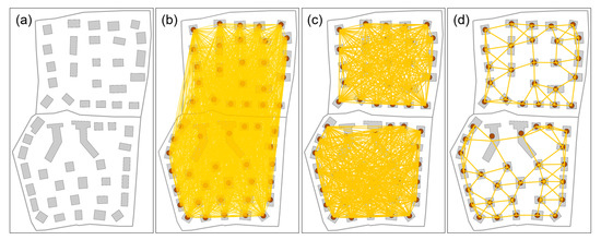
Figure 1.
Graph construction for input buildings: (a) original buildings, (b) fully connected graph, (c) graph after removing the edges that intersect the roads, and (d) four-nearest neighboring graph.
Let S = [sij]m×m denote the similarity matrix of a set of original buildings B = {b1, b2, …, bm} (m > 1), where sij (0 < i < m, 0 < j < m) represents the similarity between buildings i and j. We initially build a fully connected graph G = (V, E), where vertex vi ∈ V represents building bi and edge eij ∈ E describes the connection between buildings bi and bj (bi, bj ∈ B). Next, all edges of graph G that intersect with roads are removed, and for each vertex in graph G, only edges that connected with its k-nearest neighbors are retained. For example, in the illustrated graph in Figure 1, k is set to 4. Finally, if edge eij exists, the similarity sij (i ≠ j) is assigned to the Euclidean distance dis(vi, vj) between the centroids of bi and bj. Otherwise, it is assigned to , meaning that the corresponding two buildings are far away and cannot possibly be part of the same cluster.
2.1.2. Setting of the Preference Parameter
In the diagonal of S, elements sii (i = 1, 2,…, m) are the input values called the preference. As an important control parameter in the AP algorithm, the influence of preference values on the final clustering result is reflected in two aspects: (Ⅰ) the larger the preference value with respect to building bi (i.e., sii), the higher the possibility that bi is to be chosen as an exemplar; (Ⅱ) the larger the average value of all preferences, the larger the number of generated clusters.
Preference is usually set to a uniform value, indicating that all input objects are regarded equally as potential exemplars. In the case of building typification, however, buildings that are geometrically or semantically significant should be arranged with large preference values. This gives these buildings greater opportunity to be identified as exemplars and further retained on the generalized representation. To satisfy such requirements, a new mechanism for preference initialization was proposed. For each building bi, the preference value sii is computed as
where is a base preference value the same for all buildings, and li (0 ≤ li ≤ 1) is the importance value of bi. Those two parameters have different effects on the final clustering result. Parameter mainly controls the number of clusters, that is, the number of generated clusters increases with it. Parameter li influences the determination of clustering exemplars in local areas. The larger the value of li, the more likely the building bi is to be selected as an exemplar. In practice, the value of li can be flexibly set by users according to their generalization needs.
2.1.3. Message Propagation
As depicted in Figure 2, two kinds of messages are exchanged between connected buildings to search for appropriate clusters and their exemplars. One message is represented as the responsibility matrix R = [rik]m×m, in which rik is sent from building bi to candidate exemplar building bk. The value of rik reflects the accumulated evidence for how suited bk is to serving as the exemplar for bi while considering other potential exemplars for bi. Another type of message is represented as the availability matrix A = [aik]m×m, in which aik is sent from candidate exemplar bk to bi. The value of aik reflects the degree of how appropriate it would be for bi to choose bk as its exemplar while considering the support from other buildings that bk should be an exemplar.
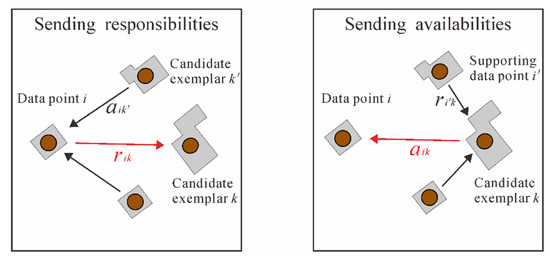
Figure 2.
Two types of messages: responsibility and availability.
The clustering process is executed as a competition that updates responsibilities and availabilities iteratively. In each iteration, the matrices R and A are updated with the results of the previous round. The rules for updating are defined as follows:
where t denotes the number of iterations and λ is the damping factor that ranges from 0 to 1. The responsibilities and the availabilities are updated repeatedly to search for a set of exemplars that maximizes the sum of similarities between each building and its exemplar.
The iterative update process is stopped when the exemplar sets are no longer changed over consecutive iterations or the predefined maximum number of iterations is reached. Then, clusters and their exemplar clustering results can be outputted based on R and A. For each building bi, we search for k that maximizes aik + rik. If k is equal to i, bi is labeled as an exemplar; otherwise, bk is identified as the exemplar for bi. Finally, the clustering results are derived according to the obtained exemplars and their members.
2.1.4. Output Generation
Since each building cluster is replaced by its exemplar on the generalized representation, the size of output clusters should be consistent with the theoretical number of buildings for the requested scale. As an unsupervised clustering algorithm, however, the number of clusters is implicitly affected by parameter . An iterative strategy was adopted to overcome this gap. Specifically, a factor (0 < < 1) is introduced to adjust the value of gradually so that the number of output clusters approaches the desired number and the difference is controlled within a certain range. The complete AP clustering-based building clustering approach is described below.
The AP-based building clustering Algorithm 1.
| Algorithm 1 |
| Input: Original buildings B = {b1, b2, …, bm} (m > 1) and their importance values L = {l1, l2,…, lm}, the base preference value
, the theoretical number of clusters n0, the adjustment factor μ, the damping factor λ, and the maximum number of iterations tmax. Output: Clusters C = {C1, C2, …, Cn} and their exemplars Z = {Z1, Z2, …, Zn}. |
|
2.2. Representation of Exemplar Buildings
Regarding the position, it is reasonable to represent each building cluster as its exemplar that is chosen as the cluster center. However, other geometric attributes of each exemplar building, including size, shape, and orientation, need to be adjusted according to the characteristics of the whole building group, as well as the changes in the scale. In addition, the importance of the exemplar building in each cluster should be considered in the determination of the typified representation. Therefore, two types of building cluster are identified with respective typified representations generated in different ways to highlight the importance of the exemplar building in each cluster, as depicted in Figure 3.
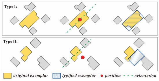
Figure 3.
Two types of building cluster and their exemplar building representations.
Type Ⅰ: The exemplar of this cluster is an important building.
For this type of cluster, the position of the exemplar building remains unchanged and its shape is characterized by a building simplification algorithm [2] to maintain the main geometrical characteristics on the target scale. In this process, the simplified representation for the typified exemplar building should satisfy the constraint that the shortest edge meets the threshold (e.g., 0.3 mm) on the target scale. Note that in this type of cluster, a few important buildings may not be chosen as an exemplar. The AP algorithm is robust in selecting exemplars that are highly reflective of the spatial distribution. Therefore, only the importance of the exemplar is emphasized in the typified representation.
Type Ⅱ: The exemplar of this cluster is not an important building.
For this type of cluster, a new building located in the centroid of the cluster is created based on the characteristics of the whole building group. Let C denote a type Ⅱ cluster that contains buildings {b1, b2, …, bm} (m > 1), and let bk () be the exemplar of cluster C. The attributes of the new building bnew are determined as follows:
- Shape: The shape of the new typified building is represented as a rectangle, since buildings located in residential suburban or rural areas are simplified significantly when the scale becomes smaller than 10k. Furthermore, the elongation of the newly created rectangle is inherited from the Minimum Bounding Rectangle (MBR) of the building with the largest area in the cluster.
- Size: The size of the new building is determined as the average area of all buildings in the cluster. That is, the created rectangle is arranged with area , where denotes the area of building .
- Orientation: The orientation of the new typified building also coincides with the average orientation of all buildings in the cluster. In this study, the orientation of a building is defined as the deviation angle between the x-axis and the long side of its MBR. Therefore, the orientation of the new rectangle, denoted as , is computed as . Here, represents the orientation of building .
Note that the newly created building may be smaller than threshold Smin (e.g., 0.6 mm × 0.4 mm), which is the size of the smallest building represented on maps. To satisfy this requirement, any new building below the threshold is amplified.
3. Results
In this section, a series of experiments with real-life building data were conducted to validate the proposed method and discuss its advantages and limitations as compared to the existing building typification methods.
3.1. Experimental Data and Parameter Setting
The present study investigated a set of buildings in a residential suburban area of Staig, Baden-Württember, Germany, captured from a topographic map. The study area is approximately 1.2 × 0.8 km2 and contains 383 buildings, as shown in Figure 4. The maximum and average areas of buildings in the dataset are 4852.0 m2 and 381.9 m2, respectively.
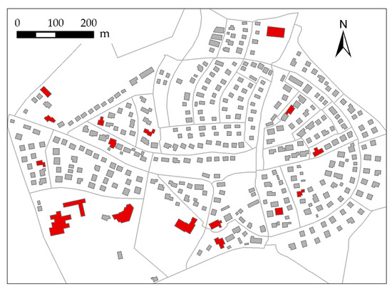
Figure 4.
Experimental data used for the validation of the proposed approach. Buildings rendered in red are important buildings.
As rendered in red in Figure 4, buildings that are prominent in size or convey specific semantics, such as a hospital or school building, were labeled as important objects. The importance values of these buildings were set to 1 in the initialization of the preference parameter, so that as many as possible would be retained during typification. The rest of the buildings were assigned importance values of 0, and parameter δ was set to the median of the pairwise similarities. The damping factor λ was set to 0.7 by the trial-and-error approach to alleviate the possible oscillations. The maximum number of iterations t-max and the preference adjustment step were set to 300 and 0.01, respectively, according to the preliminary results.
For the number of buildings retained after typification, a reasonable solution is to apply the extended radical law [12] to calculate the retention ratio for a given target scale. However, this process requires a smaller scale generalization result as a reference. For simplicity, we chose three fixed retention ratios, i.e., 70%, 50%, and 30%, to verify the proposed method.
For comparison, we implemented an unconstrained AP clustering-based algorithm, that is, the semantic meanings of buildings and the road network were not considered. In addition, the Mesh typification method [15] and the SOM typification method [16] were also implemented. As mentioned earlier, they are both global typification methods. In the SOM typification, each building was regarded as a neuron containing two features: the x and y coordinates of the building’s centroid.
3.2. Experimental Results and Analyses
3.2.1. Experimental Results
Figure 5 presents the typification results produced by the proposed method and the three comparison methods. Table 1 lists the number of buildings and important buildings retained in each result.
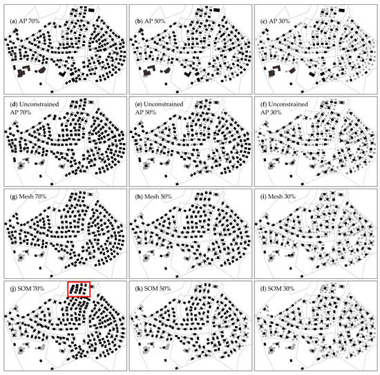
Figure 5.
Typification results of. (a–c) the AP method with retention ratios of 70%, 50%, and 30% respectively; (d–f) the unconstrained AP method with retention ratios of 70%, 50%, and 30% respectively; (g–i) the Mesh method with retention ratios of 70%, 50%, and 30% respectively; (j–l) the SOM method with retention ratios of 70%, 50%, and 30% respectively. Gray polygons denote the original buildings, and black polygons denote the typified buildings.

Table 1.
Numbers of buildings and important buildings retained in the results produced by the four methods. The values in parentheses indicate the numbers of buildings expected to be retained, with all important buildings expected to be retained in any retention ratio.
The four methods effectively screened out a part of buildings given the proportions of retained buildings and achieved visual simplification. Table 1 shows that the number of buildings retained by the Mesh method was consistent with expectations, while the number of buildings retained by the other three methods deviated from expectations. This is because the number of clusters cannot be specified for the two AP methods. An iterative approach was used in this study to control the number of outputs, and the difference from the expected was guaranteed to be within 10. For the SOM methods, the reason is that some neurons in the output layer were too weak to be activated, resulting in no building being assigned to the class represented by that neuron and the output result being less than expected. This process is difficult to control, so the SOM method cannot guarantee a difference from the expected value.
It is clear from Table 1 that the constrained AP method performed better than the Mesh and SOM methods in the preservation of important buildings. This is because the mechanism allows us to set the preference values flexibly, which enables a building with a larger importance value to have greater opportunity to be identified as an exemplar in a local cluster and, further, to be retained in the reduction of scale. On the other hand, the Mesh and SOM methods assume that the input buildings are equally important; thus, they have the same possibility to be retained in the target representation. This observation can also be verified by the comparison with the unconstrained AP method, that is, the performance of the AP method was only close to that of the Mesh and SOM methods in terms of the preservation of important buildings when the semantic meaning of buildings was not considered.
A close inspection of Figure 5 shows that the density distribution of building clusters coincides with the distribution of the original buildings. That is, in dense areas, more buildings were deleted, but the density of retained buildings was still higher than that of other areas. In the compared methods, however, buildings in dense areas were deleted relatively less. For example, when retaining 70% of the input buildings, the buildings in the upper area of the typification results produced by the SOM method were largely preserved (marked by the red rectangle in Figure 5j), which caused visual confusion on the small target scale.
Due to the constraints of the road network, buildings located on both sides of the roads were not grouped together in the AP method. However, this was not achievable in the Mesh and SOM methods. For example, when retaining 50% of the input buildings, different degrees of road conflicts occurred in the results produced by the Mesh and SOM methods, as well as those by the unconstrained AP method (Figure 6b–d). This does not satisfy the specifications of cartographic generalization and is the key criterion for users to evaluate the generalization result. Further, it may lead to the destruction of local distribution characteristics. For example, in the typification result produced by the AP method (Figure 6a), buildings are uniformly distributed on both sides of the road in a linear pattern, which is consistent with the original distribution pattern. However, the buildings are distributed in a curvilinear pattern in the results of the Mesh and SOM methods (Figure 6c,d), which destroys the original trend characteristics.
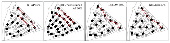
Figure 6.
Preservation of the local structural characteristics along the roads by: (a) the AP method, (b) the unconstrained AP method, (c) the Mesh method, and (d) the SOM method, respectively, with 50% retention ratio. Gray polygons denote the original buildings, black polygons denote the typified buildings, and red lines denote the structural patterns formed by the buildings.
3.2.2. Preservation of the Overall Distribution Characteristics
To better compare the performance of different approaches, we used a density map to quantify the preservation of the overall distribution characteristics. The whole region of data was divided into grid cells with the same size of 10 × 10. Then, a statistical evaluation indicator describing the density of the ith grid cell was computed by
where represents the number of buildings located in the ith grid cell. Figure 7 provides a closer visualization of the typification results that retain 70%, 50%, and 30% of the buildings using the four methods.
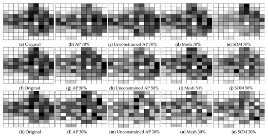
Figure 7.
Visual comparison of spatial structure preservation: (a) density distribution of original buildings; (b–e) density distributions of the typified buildings by the AP method, the unconstrained AP method, the Mesh method, and the SOM method, respectively, with 70% retention ratio; (f) density distribution of original buildings; (g–j) density distributions of the typified buildings by the AP method, the unconstrained AP method, the Mesh method, and the SOM method, respectively, with 50% retention ratio; (k) density distribution of original buildings; (l–o) density distributions of the typified buildings the AP method, the unconstrained AP method, the Mesh method, and the SOM method, respectively, with 30% retention ratio.
In the comparison, the AP method maintained the density distribution well for different proportions of retained buildings. However, both the Mesh and SOM methods caused relatively large change in the density distribution. For example, when retaining 30% of the buildings, the density of the upper areas was reduced significantly in the typification results of the Mesh method. When retaining 70% of the buildings, the density of the upper right areas in the SOM typification results was higher than that in the lower left, which is obviously different from the original density distribution. Without considering the constraints, the density distribution was maintained well when 70% of buildings were retained. However, when only 50% or 30% of buildings were retained, the density changes were more significant than those of the results with constraints. This proves that the consideration of constraints is crucial in the AP clustering-based method.
Furthermore, we propose a Relative Density Difference Index (RDDI) to quantitatively describe the density changes before and after typification, which is defined as
where and are the densities of the ith grid cell before and after typification, respectively. The density difference increases with RDDI. Table 2 lists the RDDIs of the four methods with retention ratios of 70%, 50%, and 30%.
Table 2.
RDDI values of the typification results produced by the four methods.
Table 2 shows that the RDDI of the four methods decreased as the ratio of retained building increased, meaning that the overall density change was improved. It was also observed that at each ratio, the RDDI of the typification results produced by the AP method was less than that by the Mesh and SOM methods. This comparison proves the superiority of the AP method over the two contrast methods. The RDDI of the typification result of the AP method was slightly lower than that of the unconstrained AP method when 70% of buildings were retained. However, when retaining 50% or 30% of buildings, the values were higher than that of the unconstrained AP method. This result is consistent with the previous analysis.
3.2.3. Parametric Sensitivity Analysis
In addition to evaluating the typification results, the analysis of relevant parameters also measures the effectiveness of the proposed method from the algorithmic level. The most important parameter of the AP algorithm is the damping factor , which controls whether the algorithm converges. We took the retention ratio of 50% as an example and set the maximum number of updates on the information matrix in the AP clustering to 500. Figure 8 shows the update times required for the model to perform the AP clustering as the damping factor varied.
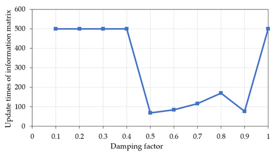
Figure 8.
Influence of the damping factor on the update times of the information matrix.
It was observed that the AP algorithm converged after 100 to 200 iterations of the information matrix as the damping factor ranged from 0.5 to 0.9. When the damping factor was less than 0.5, large weights of the matrix in the previous round resulted in slow convergence. Therefore, the AP algorithm had not converged when the update time reached the maximum. When the damping factor was larger than 0.9, the clustering results fluctuated and did not easily converge. As a result, it is necessary to select an appropriate damping factor so that the AP clustering converges quickly and steadily.
3.3. Discussion on the Advantages and Limitations of the Proposed Approach
This paper proposes a building typification approach that uses an unsupervised message passing algorithm to select appropriate exemplars. It is data-driven and has several advantages in theory and practice. First, the proposed method effectively maintains the original spatial distribution characteristics of the buildings after typification, which benefits from the competition mechanism and message propagation in the AP clustering algorithm. In contrast, the SOM method may retain redundant buildings in dense areas, while the Mesh method may lose some key features. Second, the proposed method allows us to customize the importance of individual buildings. The algorithm embeds semantic information effectively in addition to spatial characteristics, giving users the flexibility to develop diversified typification solutions according to practical needs. Third, the proposed method avoids spatial conflicts by properly dealing with the relationship between the buildings and other geographic features such as roads. The other two methods focus only on the buildings without dealing with the conflicts between other features. This violates the cartographic specifications and is likely to destroy the local structural patterns.
The proposed AP clustering-based method also has some shortcomings. First, in terms of quantity change, the AP clustering controls the number of retained buildings through iteration. The output number of exemplars may be slightly different from that expected. Additionally, the experiment revealed that properly selecting the damping factor is key in applying the method. If the damping factor is too large or too small, the clustering may not converge, so the parameters may need to be adjusted several times in practice.
4. Conclusions
In this study, we developed a global typification method based on affinity propagation exemplar-based clustering, which provides a novel algorithm from a global perspective to solve the scale transformation of buildings with many-to-many relationships in cartographic generalization. Our experiments showed that the proposed method has certain advantages over the other two global typification methods, namely, the Mesh and SOM methods, in retaining important individual buildings and preserving overall density characteristics and local structural patterns. However, there are still deficiencies in terms of the quantity control and parameter dependence.
This study focused on the typification of buildings in suburban or rural areas at a small or medium target scale. In future work, more efforts will be devoted to building generalization in other scenarios, as well as the selection of networking objects such as roads and rivers.
Author Contributions
Xiongfeng Yan and Huan Chen contributed equally. Conceptualization, Min Yang and Xiongfeng Yan; methodology, Xiongfeng Yan, Huan Chen and Min Yang; data collection, Huan Chen and Xiongfeng Yan; experiments and formal analysis, Xiongfeng Yan, Huan Chen and Haoran Huang; writing, Xiongfeng Yan, Huan Chen, Min Yang and Qian Liu; funding acquisition, Xiongfeng Yan and Min Yang. All authors have read and agreed to the published version of the manuscript.
Funding
This research was funded by the National Natural Science Foundation of China, grant numbers 42071450, 42001415.
Institutional Review Board Statement
Not applicable.
Informed Consent Statement
Not applicable.
Data Availability Statement
The data that support the findings of this study are available in Figshare at https://figshare.com/s/43e43b5f17ed2e702cef (accessed on 22 October 2021).
Acknowledgments
We would like to thank the three anonymous reviewers for their useful comments and suggestions, which greatly improved the original version of the manuscript.
Conflicts of Interest
The authors declare no conflict of interest.
References
- Deng, M.; Tang, J.; Liu, Q.; Wu, F. Recognizing building groups for generalization: A comparative study. Cartogr. Geogr. Inf. Sci. 2018, 45, 187–204. [Google Scholar] [CrossRef]
- Li, Z.; Yan, H.; Ai, T.; Chen, J. Automated building generalization based on urban morphology and Gestalt theory. Int. J. Geogr. Inf. Sci. 2004, 18, 513–534. [Google Scholar] [CrossRef]
- Shen, Y.; Ai, T.; Li, W.; Yang, M.; Feng, Y. A polygon aggregation method with global feature preservation using superpixel segmentation. Comput. Environ. Urban Syst. 2019, 75, 117–131. [Google Scholar] [CrossRef]
- Yan, X.; Ai, T.; Yang, M.; Tong, X.; Liu, Q. A graph deep learning approach for urban building grouping. Geocarto Int. 2020, 1–24. [Google Scholar] [CrossRef]
- Ai, T.; Zhang, X.; Zhou, Q.; Yang, M. A vector field model to handle the displacement of multiple conflicts in building generalization. Int. J. Geogr. Inf. Sci. 2015, 29, 1310–1331. [Google Scholar] [CrossRef]
- Bader, M.; Barrault, M.; Weibel, R. Building displacement over a ductile truss. Int. J. Geogr. Inf. Sci. 2005, 19, 915–936. [Google Scholar] [CrossRef]
- Li, W.; Ai, T.; Shen, Y.; Yang, W.; Wang, W. A novel method for building displacement based on multipopulation genetic algorithm. Appl. Sci. 2020, 10, 8441. [Google Scholar] [CrossRef]
- Mao, B.; Harrie, L.; Ban, Y. Detection and typification of linear structures for dynamic visualization of 3D city models. Comput. Environ. Urban Syst. 2012, 36, 233–244. [Google Scholar] [CrossRef]
- Regnauld, N. Contextual building typification in automated map generalization. Algorithmica 2001, 30, 312–333. [Google Scholar] [CrossRef]
- Shen, J.; Fan, H.; Mao, B.; Wang, M. Typification for façade structures based on user perception. ISPRS Int. J. Geo-Inf. 2016, 5, 239. [Google Scholar] [CrossRef] [Green Version]
- Töpfer, F.; Pillewizer, W. The principles of selection. Cartogr. J. 1966, 3, 10–16. [Google Scholar] [CrossRef]
- Burghardt, D.; Cecconi, A. Mesh simplification for building typification. Int. J. Geogr. Inf. Sci. 2007, 21, 283–298. [Google Scholar] [CrossRef]
- Gong, X.; Wu, F. A typification method for linear pattern in urban building generalisation. Geocarto Int. 2018, 33, 189–207. [Google Scholar] [CrossRef]
- Wang, X.; Burghardt, D. A typification method for linear building groups based on stroke simplification. Geocarto Int. 2021, 36, 1732–1751. [Google Scholar] [CrossRef]
- Wang, X.; Burghardt, D. A mesh-based typification method for building groups with grid patterns. ISPRS Int. J. Geo-Inf. 2019, 8, 168. [Google Scholar] [CrossRef] [Green Version]
- Sester, M. Optimization approaches for generalization and data abstraction. Int. J. Geogr. Inf. Sci. 2005, 19, 871–897. [Google Scholar] [CrossRef]
- Wang, L.; Guo, Q.; Liu, Y.; Sun, Y.; Wei, Z. Contextual building selection based on a genetic algorithm in map generalization. ISPRS Int. J. Geo-Inf. 2017, 6, 271. [Google Scholar] [CrossRef]
- Frey, B.J.; Dueck, D. Clustering by passing messages between data points. Science 2007, 315, 972–976. [Google Scholar] [CrossRef] [PubMed] [Green Version]
- Leone, M.; Weigt, M. Clustering by soft-constraint affinity propagation: Applications to gene-expression data. Bioinformatics 2007, 23, 2708–2715. [Google Scholar] [CrossRef] [PubMed] [Green Version]
- Xie, X.; Wu, F. Automatic video summarization by affinity propagation clustering and semantic content mining. In Proceedings of the International Symposium on Electronic Commerce and Security, Guangzhou, China, 3–5 August 2008; pp. 203–208. [Google Scholar]
- Kazantseva, A.; Szpakowicz, S. Linear text segmentation using affinity propagation. In Proceedings of the Conference on Empirical Methods in Natural Language Processing, Edinburgh, Scotland, UK, 27–31 July 2011; pp. 284–293. [Google Scholar]
Publisher’s Note: MDPI stays neutral with regard to jurisdictional claims in published maps and institutional affiliations. |
© 2021 by the authors. Licensee MDPI, Basel, Switzerland. This article is an open access article distributed under the terms and conditions of the Creative Commons Attribution (CC BY) license (https://creativecommons.org/licenses/by/4.0/).