Abstract
Many researchers have unraveled innovative ways of examining geographic information to better understand the determinants of crime, thus contributing to an improved understanding of the phenomenon. Property crimes represent more than half of the crimes reported in Portugal. This study investigates the spatial distribution of crimes against property in mainland Portugal with the primary goal of determining which demographic and socioeconomic factors may be associated with crime incidence in each municipality. For this purpose, Geographic Information System (GIS) tools were used to analyze spatial patterns, and different Poisson-based regression models were investigated, namely global models, local Geographically Weighted Poisson Regression (GWPR) models, and semi-parametric GWPR models. The GWPR model with eight independent variables outperformed the others. Its independent variables were the young resident population, retention and dropout rates in basic education, gross enrollment rate, conventional dwellings, Guaranteed Minimum Income and Social Integration Benefit, purchasing power per capita, unemployment rate, and foreign population. The model presents a better fit in the metropolitan areas of Lisbon and Porto and their neighboring municipalities. The association of each independent variable with crime varies significantly across municipalities. Consequently, these particularities should be considered in the design of policies to reduce the rate of property crimes.
1. Introduction
Crime rates have been declining in Western countries since the 1990s, particularly property crimes [1]. Nevertheless, crime is considered one of the phenomena that most contributes to a climate of insecurity experienced in society, and it negatively affects life satisfaction across Europe [2]. Portugal has one of the lowest crime rates among Western countries. According to the Annual Internal Security Report [3], property crimes constitute the largest share of total crimes committed in Portugal, representing 51.4% of all reported crimes in 2019.
There is a growing number of studies related to criminal activity in Portugal, such as local policies and urban security [4,5,6], criminal justice [7,8], victimization [9,10], and gender studies [11,12]. However, there is a paucity of studies on the geography of crime for Portugal, most likely due to the lack of open data with finer spatial resolution, such as point, neighborhood, or parish data. Despite the availability of socioeconomic and demographic data having increased in the last decade, only a few recent publications analyzed spatial crime patterns or addressed the relationship between crime and environmental characteristics in Portugal.
Rajcic [13] used a multidimensional descriptive data analysis technique to show that spatial crime patterns changed between 1995 and 2013 in Portuguese NUTS III regions. Macedo [14] investigated crime determinants in the municipalities of continental Portugal between 2004 and 2012, using spatial autoregressive models, and concluded that low population density has a significant positive impact on property crimes. In an exploratory study, Costa and Costa [15] applied a GWR model to crime incidence data in 86 municipalities of the north of Portugal in 2015. The results indicate that poverty, measured by ‘beneficiaries of the Social Integration Income’ has a higher impact on rural regions than on more densely urbanized municipalities. Amaral [16] used the Risk Terrain Modeling methodology [17] to identify areas where residential burglary is most likely to occur in the Police Division of Loures city located in Lisbon’s metropolitan region. The risk factors used in the model are consistent with the literature, and the results show that the location of fueling stations, educational establishments, food and beverage businesses, and bus stops are associated with areas that are vulnerable to residential burglaries.
This study aims to contribute to improved knowledge on the relationship between property crime and the demographic and socioeconomic characteristics of each municipality of mainland Portugal. Poisson-based regression models are used for this purpose, and spatial effects in crime rates are also investigated.
The geographical analysis of different factors associated with property crimes in Portugal enables a better understanding of this phenomenon. Neto et al. [18] stressed the importance of developing demographic and crime scenarios in Portugal, and disclosed a dashboard for data visualization to support location-allocation scenarios for security forces. Our findings can be useful not only for subsequent crime studies in Portugal, but also for police authorities and city councils in the decision-making process and planning of actions adjusted to regional characteristics in crime prevention.
2. Literature on Geography of Crime Analysis
The occurrence of criminal activity is neither randomly nor uniformly distributed in space [19], and crime patterns vary according to the type of crime [20]. The routine activity theory [21] and the crime pattern theory [22] do not seek to explain crime geography based on the characteristics of criminals but rather through the specific environment and context in which crimes occur. The routine activity theory asserts that motivated offenders, desirable targets, and the lack of effective security are three important crime determinants. This theory supported many studies on residential burglary [23]. The rational choice theory and the crime pattern theory also underline the importance of places of crime. Curtis-Ham et al. [24] propose a framework to extend these environmental criminology theories and reviews their theoretical background.
The theory of social disorganization [25] highlighted three structural factors on the geography of crime, namely social and economic deprivation, ethnic heterogeneity, and population turnover, which have been later considered in several studies (e.g., [26,27]). Sampson [28], and Sampson and Groves [29], advocated that family instability or disruption also leads to social disorganization, thus increasing crime and delinquency in urban environments. Sampson et al. [30] and Graif et al. [31] review and expand the research on neighborhood and poverty effects on urban crime. Jones and Pridemore [32] propose an extension of theoretical and methodological approaches for explaining the concentration of crime in urban environments by combining elements of the routine activities and social disorganization theories. Valuable reviews of the various theoretical contributions to these theories, which inform our analysis on the geography of property crimes in Portugal at the municipality level, are offered by Cahill and Mulligan [26], Wickes [33], and Kubrin and Mioduszewski [34].
The relationship between environmental characteristics and crime has been widely investigated using Geographic Information Systems (e.g., [35]), data mining techniques [36], and multivariate statistical analysis (e.g., [37,38]). Spatial dependence and spatial heterogeneity violate the assumptions underlying classical regression models, and thus, these spatial effects should be addressed when modeling geographic data. In crime analysis, conventional spatial regression models dealing with spatial autocorrelation are the spatial lag and spatial error models [39,40]. A less common approach to deal with it is the Cliff–Ord spatial autoregressive model with spatial autoregressive disturbances [41]. Geographically Weighted Regression (GWR) was proposed by Fotheringham et al. [42] to deal with spatial heterogeneity. It is difficult to model both spatial effects at the same time [43], but GWR diminishes the problem of spatially autocorrelated error terms [42], and it is increasingly being used in crime analysis (e.g., [44,45,46]). Poisson or Negative Binominal regression models are more suitable for event counts [47,48], and thus, the Geographically Weighted Poisson Regression (GWPR) and the Geographically Weighted Negative Binomial Regression (GWNBR) models have been applied to address spatial effects in crime rates [49,50,51].
The key dimensions underlying the spatial variability of crimes against property are primarily supported by the previously mentioned crime theories (e.g., [52,53]). The literature also highlights complex relationships between income inequality and property crime, and conflicting results on the relationships between unemployment rates/low-income factors and burglary rates [41]. Moreover, GWR models revealed a complex relationship between immigration and property crime across census tracts in Vancouver, Canada [44].
Regression does not reveal the causal relationships between variables but only disentangles the structure of the association (correlation in the case of Ordinary Least Squares) between them. The set of independent variables considered in this study was selected based on a thorough literature review and according to the routine activity theory and, mostly, from the perspective of the social disorganization theory. Explanatory variables commonly used in previous studies to model property crimes include the following: unemployment (e.g., [54]), low-income population/household income [41,53], level of education [23,51], age group [49,55], multiunit/multi-family dwellings [53,56], population density [47], residential instability [23,43], ethnic/race heterogeneity [55], and land use/built environment characteristics [35,57,58].
3. Data and Methods
Three types of Poisson regression models were used and compared based on goodness-of-fit measures. The Global Poisson model was estimated for the purpose of comparison with models that are able to deal with the spatial nonstationary relationship between property crimes and its predictors, namely the local Geographically Weighted Poisson Regression (GWPR) and the semi-parametric GWPR (S-GWPR). The following sections briefly describe the variables considered in this study and the Poisson-based regression models estimated with the GWR 4.09 software [59].
A multicollinearity check between independent variables was conducted. Spatial autocorrelation in property crime rates was assessed with the Global Moran’s I statistic, and spatial heterogeneity was investigated with the Local Moran’s I statistic and the Getis–Ord Gi* statistic in ArcGIS 10.6 software.
3.1. Study Area and Data
The study area is mainland Portugal, and municipalities are the spatial units of all analyses. Data from the year 2017 were collected from official sources, namely the Directorate-General for Education and Science Statistics (DGEEC—Direção-Geral de Estatísticas da Educação e Ciência, https://www.dgeec.mec.pt, accessed on 24 August 2021), and PORDATA (https://www.pordata.pt, accessed on 24 August 2021). The year 2017 was the most recent year with available socioeconomic data for all 278 municipalities.
The 2001 and 2011 Census data show a decrease in the young population and a tendency towards an increase in the number of elderly people. In recent decades, depopulation has increased in the interior cities [60], while the western coastal territories have become denser, particularly the metropolitan areas of Lisbon and Porto. In 2017, the number of residents in mainland Portugal was estimated by Statistics Portugal at 9,801,106 people, of which 4,630,471 were men and 5,162,326 were women, and the population aging trend continued. The contrast in population density between inland and coastal municipalities is considerable. Population density varied between 4.1 and 7529.7 inhabitants/Km2 in the 278 municipalities of continental Portugal (mean = 303.7 inhabitants/Km2; standard deviation = 836.7 inhabitants/Km2). There was a considerable improvement in the level of education of the population over the past decades. Nevertheless, the estimated percentage of the resident population of mainland Portugal aged 15 and over without upper-secondary education was 60.5% in 2017, and the unemployment rate was 8.8%, according to PORDATA.
3.1.1. Crime Data
There has been a decline in the number of crimes over the past 25 years, especially violent ones, and urban areas are more likely to have higher crime rates [18]. The number of property crimes observed in 2017 varied from 15 to 24,817 at the municipality level, with a total of 163,108 reported crimes. The property crime rate per 1000 inhabitants was computed for each municipality (Figure 1). The average crime rate was 12.61, with a standard deviation of 5.93. The highest crime rates are observed in the municipalities of Lisbon, Albufeira in the Algarve region in the south, and Porto (49, 48, and 43 crimes per 1000 inhabitants, respectively), as well as in other municipalities in the Algarve region. The municipality of Valença, in the northwest region, is also one of the ten municipalities of Portugal with the highest crime rate (28 crimes per 1000 inhabitants). The lowest crime rate was registered in Proença-a-Nova (center region).
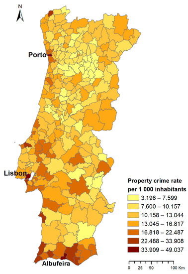
Figure 1.
Spatial distribution of property crime rates per thousand inhabitants by municipality in 2017.
3.1.2. Demographic and Socioeconomic Data
Following the literature review on the determinants of property crimes, the independent variables used in the Poisson-based regression models (Table 1) measure social inequality (Retention and dropout rates in basic education; Gross enrollment rate; Foreign population), income inequality (Purchasing power per capita; Monthly remuneration of employees), poverty (Guaranteed Minimum Income and Social Integration Benefit), Unemployment, and residential instability (Conventional dwellings). A measure of the young population was also selected to characterize offenders’ individual characteristics [61]. We did not use any variable to control for family disruption, such as lone-parent families or divorce rate, because previous studies showed that this factor is particularly important to explain the geography of violent crimes (e.g., [26,29]) and juvenile violence [62,63], but it has a much smaller effect on property crimes (e.g., [47,64]). Ethnic/race heterogeneity was not considered due to the lack of data.

Table 1.
Summary of variables, descriptive statistics, and Pearson’s correlation test with property crime rates.
All variables are significantly correlated with property crime rates at the 5% significance level, except for three variables: young resident population, Guaranteed Minimum Income and Social Integration Benefit, and unemployment rate (Table 1). A low (global) linear correlation with crimes does not mean that the local association is not high for some municipalities. Hence, those variables were only discarded from a few regression models that were investigated.
The density of conventional dwellings is higher in the metropolitan areas of Lisbon and Porto. The southern municipalities and Lisbon have a higher proportion of foreign population. Unemployment figures and the numbers of beneficiaries of income from government assistance were found to be identically distributed, which was expected since unemployed individuals usually benefit from Guaranteed Minimum Income and Social Integration Benefits. Lower amounts of monthly remuneration were observed in the inland municipalities, while northern and coastal regions showed higher rates of young resident population. Purchasing power and variables characterizing population education exhibited a dispersed pattern across municipalities.
The Variance Inflation Factor (VIF) values of the nine variables were smaller than 3, indicating no evidence of multicollinearity between them. Therefore, all of them were considered in the regression models.
3.2. Poisson-Based Regression Models
Geographically Weighted Poisson Regression (GWPR) models have been used in several studies on the geography of crime [43,51,65]. The GWPR extends the geographically weighted regression model with the Poisson distribution, as proposed by Nakaya et al. [66]. The GWPR models were used to investigate the spatial relationship between property crimes and socioeconomic and demographic variables in mainland Portugal. Additionally, the semi-parametric GWPR (S-GWPR) model was investigated. While the GWPR model is a local spatial model with varying coefficients for all independent variables, the S-GWPR includes both global and local independent variables.
Let be the number of property crimes in the municipality , and let be the j-th independent variable in the municipality . Poisson regression assumes that follows a Poisson distribution with mean given by . The property crime rate in the municipality is represented by , where is the number of inhabitants of the municipality, and its mean value is .
The Poisson regression model for property crime rate is [66]:
where denotes the natural logarithm of the expected value of the property crime rate in the municipality , is the j-th explanatory variable, and are parameters to be estimated using the maximum likelihood method. This equation can be rewritten in an equivalent way as:
The expected value of the number of property crimes in municipality i is given by:
Simplifying the previous formula, we obtain the global Poisson regression model for the number of property crimes, where is usually named the offset variable:
The spatial coordinates of point i are integrated into the general equation of the GWR model, thus allowing the relationships between independent and dependent variables to vary by location [42]. All independent variables have a local scope in GWR models because they are associated with parameters that depend on the location of municipality i, for which the equation will be estimated, using the observations of the neighboring municipalities. The GWPR model for the number of property crimes corresponds to an adaptation of the global model formulated in Equation (4):
where are the spatial coordinates of the centroid of municipality , and are continuous functions of the location .
Some of the independent variables may be spatially stationary; thus, their influence may always be the same whatever the municipality i for which Equation (5) is being estimated. This concept was formalized in the semi-parametric GWPR model, proposed by Nakaya et al. [67], which is an extension of Equation (5). This model allows for the inclusion of variables that may have a global explanatory effect (such as global models) and others whose explanatory power varies locally. The semi-parametric GWPR (S-GWPR) model is then given by:
where it is assumed that the parameter associated with the g-th independent variable does not depend on the location of municipality .
All models were investigated using the GWR4.09 software, in which the Local-To-Global algorithm was used to iteratively select global variables for the S-GWPR model [59,67].
The estimation of the parameters was performed through a spatial weighting function that can be fixed or variable (i.e., based on a fixed or adaptive kernel). This function is based on distance so that municipalities closest to municipality i have more influence on the estimation of these parameters. In general, when the polygons that define the spatial units (i.e., the municipalities) have different sizes, it is preferable to use an adaptive kernel so that the bandwidth parameter of the spatial weighting function can vary according to the density of the data. Consequently, the number of neighboring municipalities to consider in each local regression (Equations (5) and (6)) is optimized. The bi-square kernel with adaptive bandwidth is one of the most frequently used weighting functions, and it was used in this study:
where corresponds to the weight assigned to the observation of municipality j for estimating the coefficient at the municipality i location, represents the Euclidean distance between the centroids of municipalities and , and is the adaptive bandwidth size defined as the k-th nearest neighbor distance to location i [59]. The optimal bandwidth size was determined by means of comparison of the AICc (small sample bias-corrected Akaike Information Criterion) of models with different bandwidth sizes. This strategy is recommended for local regression models to account for small degrees of freedom [66].
The comparison between Poisson models was made considering the AICc formulation proposed by Nakaya et al. [66]. The lower the AICc, the better the performance of the model. We also considered the Percent of Deviance Explained as a model performance criterion. This measure in Poisson regression is analogous to the R2 value in classical linear regression; thus, the higher the Percent of Deviance Explained, the better the model fits to the data.
4. Results and Discussion
4.1. Spatial Effects in Crime Rates
Property crime rates exhibit positive spatial autocorrelation over the study region since the value of the Global Moran’s I statistic was 0.354, and it was statistically different from zero (z-score = 12.64; p-value < 0.0001). This facet means that municipalities with high crime rates correlate with high neighboring values, or municipalities with low values correlate with low neighboring values.
Figure 2 shows the distribution of significant positive (high–high and low–low clusters) and negative (high–low and low–high outliers) spatial autocorrelations for property crime rates. Local Moran’s I revealed local clusters of high–high values in southern municipalities and the Lisbon and Porto metropolitan regions, where high crime rates are surrounded by high crime rates. Many municipalities in the central area of the north and the municipalities of Reguengos de Monsaraz, Alandroal, and Estremoz (east and southeast of Lisbon) correspond to low–low clusters (i.e., these municipalities with low crime rates have neighboring municipalities with low crime rates). Furthermore, two municipalities near Lisbon (Vila Franca de Xira and Odivelas) and Monchique in the south correspond to low–high spatial outliers, where low values correlate with high neighboring values. The municipalities of Montalegre, Braga, Felgueiras, Mesão Frio, Viseu, Celorico da Beira, Seia, Coimbra, Góis, Castanheira de Pêra, and Évora have high crime rates surrounded by low crime rates; thus, they are depicted as high–low spatial outliers.
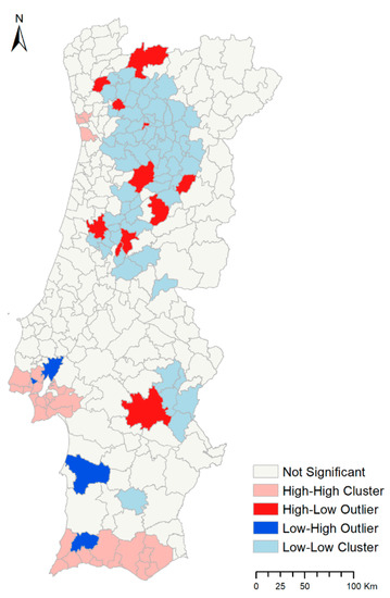
Figure 2.
Results of the Local Moran’s I statistic for property crime rates per thousand inhabitants by municipality in 2017.
The Getis–Ord Gi* statistic was used to identify the locations of statistically significant clusters with either high (hot spot) or low (cold spot) values (Figure 3). As expected from the previous analyses, the metropolitan regions of Lisbon and Porto, as well as the Algarve region in the south, stand out as clusters with high property crime rates. The north region displays a cluster of low crime rates with 43 municipalities (at significance levels smaller than or equal to 10%). Additionally, the municipalities of Santa Comba Dão, Penacova, Tábua, Condeixa-a-Nova, Lousã, Miranda do Corvo, Góis, Castanheira de Pêra, Proença-a-Nova, Estremoz, Alandroal, and Reguengos de Monsaraz are included in other cold spot clusters.
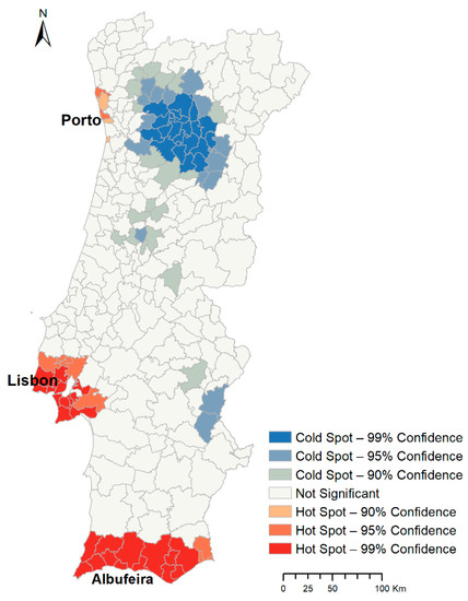
Figure 3.
Results of the Getis–Ord Gi* statistic for property crime rates per thousand inhabitants by municipality in 2017.
4.2. Model Performance Comparison
Both stationary and nonstationary spatial relationships between property crimes and driving factors were investigated with S-GWPR models. The Local-To-Global algorithm revealed no improvement in the modeling when the nine independent variables (Table 1) were iteratively selected as global variables for the S-GWPR models because the lowest AICc (2937.661) was obtained before variable selection. Hence, the S-GWPR models were not further analyzed.
Different combinations of five to nine independent variables were included in the seventeen global and local GWPR models investigated (Table 2). Models 2 to 17 were given fewer predictor variables than model 1 in order to reduce the number of parameters being estimated. The excluded variables were selected because they measure a crime factor that is also characterized by another variable included in the model and/or they have a lower correlation with property crime rates. Table 2 details the goodness-of-fit measures of those models, where the results are arranged in decreasing order of the AICc values of the GWPR models. As expected, all the GWPR models have smaller values of the AICc than the global Poisson regressions, thus revealing a better fit. The Percent of Deviance Explained was also considerably improved in all GWPR models when compared to the global models. The GWPR model 8 was considered the best-fit model because its adjustment measures are similar to those of GWPR model 1, which has the smallest AICc, but the GWPR model 8 is more parsimonious as it only incorporates eight predictors. All parameter estimates of the Global Poisson model 8 are significant except ‘Conventional dwellings’ (Table 3).
Table 2.
Goodness-of-fit measurements for global and local Poisson regression models.
Table 3.
Statistics of Global Poisson regression and GWPR for model 8.
The Local Percent of Deviance Explained map (Figure 4) shows that the GWPR model 8 has greater explanatory power in the municipalities of the metropolitan regions of Lisbon and Porto. On the other hand, the model fit is lower in the municipalities of Vila Pouca de Aguiar, Vila Real, Santa Marta de Penaguião, Fundão, Idanha-a-Nova, Castelo Branco, Vila Velha de Ródão, Marinha Grande, Alcobaça, Nazaré, Porto de Mós, and Batalha.
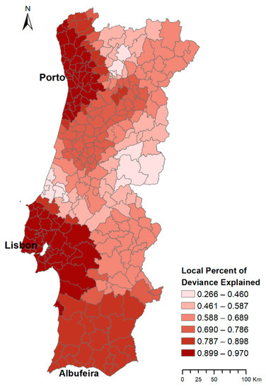
Figure 4.
Local Percent of Deviance Explained of the best-fit model (GWPR model 8).
4.3. Spatial Analyses of the Coefficients
The coefficients of the best-fit model (GWPR model 8) show the existence of non-stationarity through different spatial patterns of the local coefficients of each independent variable. In Figure 5, these coefficients are shown for municipalities where the pseudo t-values are high (), indicating that local relationships with property crimes occurrence may be significant at the 5% level [66]. There are several local coefficients varying from negative to positive values. Chen et al. [49] argue that such a pattern might be explained by not considering overdispersion in GWPR. The spatial patterns of local coefficients may also be influenced by the spatial aggregation level of the data, which might not capture the heterogeneity of the phenomena properly.
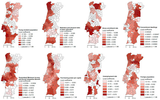
Figure 5.
Local coefficients of the best-fit model (GWPR model 8).
The coefficients of the young resident population are negative in northern municipalities and are positive in the south and in the metropolitan region of Lisbon (Figure 5), where they are higher in Sintra, Cascais, and Oeiras, which are municipalities with high property crime rates. Based on the routine activity theory, it was expected that this variable would have a positive impact on crime [68] because young age groups are often affected by low income and unemployment, thus generating conflicts and inequalities, and making them prone to opportunities that can generate increased criminal occurrences.
Retention and dropout rates in basic education have a positive association with property crimes in most of the study region (Figure 5). This result was expected from the theory of social disorganization [51], considering the complementarity between dropping out of school, disadvantageous education attainment, and the practice of criminal activities. This variable has a higher positive impact in the northwest municipalities, particularly in Valença, Monção, and Vila Nova de Cerveira, located in the Viana do Castelo district.
The spatial pattern of conventional dwellings is similar to that of population density. Therefore, municipalities located in coastal regions (west and south) have a larger density of conventional dwellings than those located in rural regions. This variable shows positive coefficients in most of the study region (Figure 5), particularly in the rural municipalities of the northeast such as Penalva do Castelo, Aguiar da Beira, and Fornos de Algodres. These results may be explained by a higher number of vacant houses (i.e., not being used for all or part of the year) in the rural interior [69], thus making them attractive targets for burglary [70].
The variable ‘Guaranteed Minimum Income and Social Integration Benefit’ measures poverty, and ‘purchasing power per capita’ characterizes income inequality. The former shows a positive relationship with property crime in many municipalities (Figure 5), particularly in Lisbon and its neighboring municipalities (especially in Sesimbra, Seixal, and Barreiro in the Setúbal district) as well as in the northwest. Contrariwise, a few municipalities in the south show small negative coefficients. Purchasing power per capita also has positive coefficients in most administrative units, but their spatial pattern is very different from those of income from government assistance. The former variable has a higher positive association in Porto and its neighboring municipalities. Moreover, purchasing power per capita has a negative relationship with property crime in a few municipalities in the northeast.
The relationship between poverty, income inequality, and crime rates is complex. Hence, it is a controversial issue that has been debated at length in the literature (e.g., [71,72,73,74]). The conclusions from different studies often seem contradictory as they depend on the type of crime, the spatial resolution of the analyses, and the methodological and empirical approach. Metz and Burdina [41] analyzed the impact of income inequality within and across census block groups in three USA cities. Their results show that property crime rates are affected by income inequality on the micro-level, and that income inequality has a determinant role in crime levels across block groups. Andresen [75] applied a decomposition model at different time frames to a panel dataset of Canadian provinces (1981–2009) and concluded that the long- and short-run effect of GPP per capita on property crime was statistically insignificant. Imran et al. [72] argue that poverty leads to property crime in the long run in the USA. In an across-countries study, Goda and Torres García [76] empirically concluded that absolute income inequality is a more significant and robust determinant of violent property crime than relative inequality. A cross-national study showed that income inequality has little or no effect on crime in Western/Southern Europe [77]. Ferreira [78] modeled annual crime records (1993–2009) in Portugal, using an autoregressive distributed lag approach, and observed a negative relationship between economic deprivation and property crimes, whereas the relationship was positive for crimes against people (except threat and coercion, and domestic violence). Beneficiaries of income from government assistance exhibited positive coefficients in a GWPR model applied to motor vehicle theft in a Mexican city [50].
The unemployment rate local coefficients have a negative sign in most of the country (Figure 5), as expected as per the Cantor and Land [79] theory, whereas they are positive in several municipalities. This variable shows a higher positive effect on property crimes in Idanha-a-Nova (Castelo Branco district in central Portugal), Santiago do Cacém (Setúbal district in the southwest), and Mourão (Évora district in the southeast). According to Cantor and Land [79], “the total effect of the unemployment rate is the sum of positive motivational and negative opportunity impacts.” They argue that the unemployment rate has a negative short-run effect on crime rates due to decreasing criminal opportunities, while an increasing unemployment trend has a positive (long-run) effect due to increased criminal motivation. Many studies addressed these issues, and their theory is still controversial. Andresen [75] considered both motivational and opportunity impacts on crime by investigating the combined effects of unemployment and economic variables at different time frames in Canadian provinces (1981–2009) and observed significant negative short- and long-run effects of unemployment on property crime. Costantini, Meco, and Paradiso [80] investigated the long-run relationship between property crime, unemployment, inequality, and deterrence activity in the USA at the state level using a nonstationary panel model (1978–2013), and their results show significantly positive long-run effects of unemployment on property crime. Using a two-way fixed effects model and twenty years of data (1990–2009), Frederick and Jozefowicz [81] found that urban counties in Pennsylvania, USA, experience both a criminal opportunity effect and a criminal motivation effect, but there was no evidence for either in rural counties.
The social disorganization theory suggests that areas where the concentration of minorities predominates are generally positively correlated with crime, presuming possible integration difficulties and social deprivation. Vilalta and Fondevila [51] found that violent crimes, mostly robberies or thefts, had a positive association with the percentage of migrants in the Santa Fe neighborhood of Mexico City at the census block level. As expected, the foreign population has a positive association with property crimes in most of the study region (Figure 5). Even though southern municipalities have a higher proportion of foreign population, the local coefficients are higher in the north, particularly in Moimenta da Beira, Penedono, and Tarouca. Conversely, they are negative in some municipalities of the Viseu district, Mealhada, and Baião.
5. Conclusions
The number of studies on the factors causing heterogeneous spatial patterns of property crime in Portugal is scant. Different Poisson-based regression models were estimated, with the aim of investigating the relationship between property crimes and the socioeconomic and demographic characteristics of municipalities in mainland Portugal in 2017. The best-fit model was the Geographically Weighted Poisson Regression model with eight independent variables (GWPR model 8), which assessed the association between property crimes and young age groups, social inequality, poverty and income inequality, and residential instability at the municipality level. The model showed greater explanatory power in the metropolitan regions of Lisbon and Porto, as well as in southern municipalities, where high crime rates are clustered.
The model made it possible to capture the existence of spatial non-stationarity in property crime data, as evidenced by the spatial distribution of the local coefficients of each independent variable (Figure 5). Hence, this study contributes to the identification of municipality-specific characteristics that are related to the occurrence of property crimes in mainland Portugal. This improved understanding of crime patterns and factors may assist in the planning of actions to mitigate crime occurrences [55]. The Crime Prevention Through Environmental Design (CPTED) approach [82] is increasingly being supported by researchers, and used by public authorities, as a valuable tool to create strategies to reduce crime through the proper design and judicious use of the built environment, such as through the differentiation of public and private property by the use of symbolic and real barriers, formal and informal surveillance, the minimization of access to potential targets, and the maximization of offenders’ perception regarding risk (e.g., [83,84]). Such environmental strategies are particularly relevant in more urbanized municipalities, such as Lisbon and Porto, and in the Algarve region, where property marking of household items and its advertising should also be encouraged to assist in the prevention of residential burglary [85]. The principles and concepts of CPTED have evolved in the last decades through the growing importance of the social characteristics of the community [86], and through the integration of human motivation and aspirations within a neighborhood [87]. The promotion of social programs and community participation could benefit the municipalities where we found a stronger association between foreign population and property crimes (e.g., Moimenta da Beira, Penedono, and Tarouca). In the northwest municipalities, particularly those of the Viana do Castelo district, the promotion of measures to reduce students’ absenteeism and local action plans to tackle poverty, among other measures of social cohesion, could contribute to reducing the incidence of crimes. Rural municipalities of the northeast, where our results showed a higher association between property crimes and conventional dwellings, could benefit from the promotion of visually permeable fencing in properties (e.g., plantings or wooden fences) and the placement of agricultural structures (e.g., storehouses) in places with enhanced visibility to improve control, accessibility, and surveillance [88]. Moreover, there is a growing amount of technology that may help law enforcement bodies overcome geographic obstacles in rural areas, such as the deployment of CCTV, security lighting, and sensing technologies [89].
The local coefficients exhibit the expected (positive or negative) sign in most of the study region, but several municipalities have coefficients with the opposite sign, which may be due to overdispersion in GWPR [49]. Future studies should investigate the application of Geographically Weighted Negative Binomial models to overcome this possible limitation.
Furthermore, data aggregated at the municipality level may hide the heterogeneity of the phenomena at more disaggregated spatial levels (e.g., the city, parish, or neighborhood) and, therefore, spatial analyzes (e.g., hot spots) and spatial regression models may fail to capture the heterogeneity of criminal occurrence and the socioeconomic factors associated with it. This limitation corresponds to the well-known Modifiable Area Unit Problem (MAUP), referred to in studies on the geography of crime [90,91]. Although there is a large body of literature on this problem, there is no general solution to it [92]. A sensitivity analysis is recommended for future studies, which was not possible in this study due to the lack of data at finer spatial scales.
Author Contributions
Conceptualization, Joana Paulo Tavares and Ana Cristina Costa; Formal analysis, Joana Paulo Tavares; Methodology, Joana Paulo Tavares and Ana Cristina Costa; Resources, Ana Cristina Costa; Software, Joana Paulo Tavares; Validation, Ana Cristina Costa; Writing—original draft, Joana Paulo Tavares and Ana Cristina Costa; Writing—review and editing, Joana Paulo Tavares and Ana Cristina Costa All authors have read and agreed to the published version of the manuscript..
Funding
This research received no external funding.
Data Availability Statement
The data used in this article are available in the references presented in Section 2.
Conflicts of Interest
The authors declare no conflict of interest.
References
- Tonry, M. Why Crime Rates Are Falling throughout the Western World. Crime Justice 2014, 43, 1–63. [Google Scholar] [CrossRef]
- Brenig, M.; Proeger, T. Putting a Price Tag on Security: Subjective Well-Being and Willingness-to-Pay for Crime Reduction in Europe. J. Happiness Stud. 2018, 19, 145–166. [Google Scholar] [CrossRef]
- Government of Portugal. Relatório Anual de Segurança Interna 2019; Sistema de Segurança Interna, Gabinete do Secretário-Geral, XXII Governo-República Portuguesa; Portuguese Republic Government: Lisboa, Portugal, 30 June 2020.
- Amante, A.; Saraiva, M.; Marques, T.S. Community Crime Prevention in Portugal: An Introduction to Local Safety Contracts. Crime Prev. Community Saf. 2021, 23, 155–173. [Google Scholar] [CrossRef]
- Saraiva, M.; Matijosaitiene, I.; Diniz, M.; Velicka, V. Model (My) Neighbourhood—A Bottom-up Collective Approach for Crime-Prevention in Portugal and Lithuania. JPMD 2016, 9, 166–190. [Google Scholar] [CrossRef]
- Tulumello, S. The Multiscalar Nature of Urban Security and Public Safety: Crime Prevention from Local Policy to Policing in Lisbon (Portugal) and Memphis (the United States). Urban Aff. Rev. 2018, 56, 1134–1169. [Google Scholar] [CrossRef]
- Gomes, S. Prison, Ethnicities and State: Establishing Theoretical and Empirical Connections; Prisons, State and Violence; Guia, M., Gomes, S., Eds.; Springer: Cham, Switzerland, 2019; pp. 49–69. [Google Scholar] [CrossRef]
- Matos, M.; Gonçalves, M.; Maia, Â. Human Trafficking and Criminal Proceedings in Portugal: Discourses of Professionals in the Justice System. Trends Organ. Crime 2018, 21, 370–400. [Google Scholar] [CrossRef]
- Martins, P.C.; Mendes, S.M.; Fernández-Pacheco, G.; Tendais, I. Juvenile Victimization in Portugal through the Lens of ISRD-3: Lifetime Prevalence, Predictors, and Implications. Eur. J. Crim. Policy Res. 2019, 25, 317–343. [Google Scholar] [CrossRef]
- Matos, M.; Grangeia, H.; Ferreira, C.; Azevedo, V.; Gonçalves, M.; Sheridan, L. Stalking Victimization in Portugal: Prevalence, Characteristics, and Impact. Int. J. Law Crime Justice 2019, 57, 103–115. [Google Scholar] [CrossRef]
- Gonçalves, M.; Ferreira, C.; Machado, A.; Matos, M. Men Victims of Stalking in Portugal: Predictors of Help-Seeking Behaviours. Eur. J. Crim. Policy Res. 2021, 1–18. [Google Scholar] [CrossRef]
- Matias, A.; Gonçalves, M.; Soeiro, C.; Matos, M. Intimate Partner Homicide in Portugal: What Are the (As) Symmetries Between Men and Women? Eur. J. Crim. Policy Res. 2020, 1–24. [Google Scholar] [CrossRef]
- Rajcic, S.T. Spatial Analysis of Crime Evolution in Portugal between 1995 and 2013. Master’s Thesis, NOVA Information Management School, Lisboa, Portugal, 2015. [Google Scholar]
- Macedo, A. Para Uma Discussão Dos Determinantes Da Criminalidade Em Portugal. Master’s Thesis, Universidade do Minho, Braga, Portugal, 2016. [Google Scholar]
- Costa, J.D.; Costa, A.C. Application of Spatial Regression to Investigate Current Patterns of Crime in the North of Portugal; Societal Geo-Innovation: Short papers, posters and poster abstracts of the 20th AGILE Conference on Geographic Information Science, Wageningen University & Research; Bregt, A., Sarjakoski, T., van Lammeren, R., Rip, F., Eds.; Wageningen University & Research: Wageningen, The Netherlands, 2017; pp. 9–12. Available online: http://hdl.handle.net/10362/75707 (accessed on 22 February 2021).
- Amaral, R.F. Avaliação Espacial Como Estratégia Mitigacional Preditiva: O Crime de Furto no Interior de Residências na Divisão Policial de Loures. MSc Dissertation, Instituto Superior de Ciências Policiais e Segurança Interna, Lisboa, Portugal, 2018. [Google Scholar]
- Caplan, J.M.; Kennedy, L.W. Risk Terrain Modeling: Crime Prediction and Risk Reduction; University of California Press: Berkeley, CA, USA, 2016. [Google Scholar]
- Neto, M.D.C.; Nascimento, M.; Sarmento, P.; Ribeiro, S.; Rodrigues, T.; Charlton, M. Implementation of a Dashboard for Security Forces Data Visualization; Associação Portuguesa de Sistemas de Informação: Guimaraes, Portugal, 2018; Available online: https://aisel.aisnet.org/capsi2018/19 (accessed on 7 July 2021).
- Lee, Y.; Eck, J.E.; SooHyun, O.; Martinez, N.N. How Concentrated Is Crime at Places? A Systematic Review from 1970 to 2015. Crime Sci. 2017, 6, 1–16. [Google Scholar] [CrossRef]
- Hayward, K.J. Five Spaces of Cultural Criminology. Br. J. Criminol. 2012, 52, 441–462. [Google Scholar] [CrossRef]
- Cohen, L.E.; Felson, M. Social Change and Crime Rate Trends: A Routine Activity Approach. Am. Sociol. Rev. 1979, 44, 608. [Google Scholar] [CrossRef]
- Brantingham, P.J.; Brantingham, P.L.; Andresen, M.A. The Geometry of Crime and Crime Pattern Theory. In Environmental Criminology and Crime Analysis; Routledge: Abington, UK, 2017; Volume 2. [Google Scholar]
- Malczewski, J.; Poetz, A. Residential Burglaries and Neighborhood Socioeconomic Context in London, Ontario: Global and Local Regression Analysis. Prof. Geogr. 2005, 57, 516–529. [Google Scholar] [CrossRef]
- Curtis-Ham, S.; Bernasco, W.; Medvedev, O.N.; Polaschek, D. A Framework for Estimating Crime Location Choice Based on Awareness Space. Crime Sci. 2020, 9, 23. [Google Scholar] [CrossRef]
- Shaw, C.R.; McKay, H.D. Juvenile Delinquency and Urban Areas: A Study of Rates of Delinquents in Relation to Differential Characteristics of Local Communities in American Cities; University of Chicago Press: Chicago, IL, USA, 1942. [Google Scholar]
- Cahill, M.E.; Mulligan, G.F. The Determinants of Crime in Tucson, Arizona. Urban Geogr. 2003, 24, 582–610. [Google Scholar] [CrossRef]
- Smith, W.R.; Frazee, S.G.; Davison, E.L. Furthering the Integration of Routine Activity and Social Disorganization Theories: Small Units of Analysis and the Study of Street Robbery as a Diffusion Process. Criminology 2000, 38, 489–524. [Google Scholar] [CrossRef]
- Sampson, R.J. Urban Black Violence: The Effect of Male Joblessness and Family Disruption. Am. J. Sociol. 1987, 93, 348–382. [Google Scholar] [CrossRef]
- Sampson, R.J.; Groves, W.B. Community Structure and Crime: Testing Social-Disorganization Theory. Am. J. Sociol. 1989, 94, 774–802. [Google Scholar] [CrossRef]
- Sampson, R.J.; Morenoff, J.D.; Gannon-Rowley, T. Assessing “Neighborhood Effects”: Social Processes and New Directions in Research. Annu. Rev. Sociol. 2002, 28, 443–478. [Google Scholar] [CrossRef]
- Graif, C.; Gladfelter, A.S.; Matthews, S.A. Urban Poverty and Neighborhood Effects on Crime: Incorporating Spatial and Network Perspectives. Sociol. Compass 2014, 8, 1140–1155. [Google Scholar] [CrossRef] [PubMed]
- Jones, R.W.; Pridemore, W.A. Toward an Integrated Multilevel Theory of Crime at Place: Routine Activities, Social Disorganization, and the Law of Crime Concentration. J. Quant. Criminol. 2019, 35, 543–572. [Google Scholar] [CrossRef]
- Wickes, R. Social Disorganization Theory: Its History and Relevance to Crime Prevention. In Preventing Crime and Violence; Teasdale, B., Bradley, M.S., Eds.; Springer International Publishing: Cham, Switzerland, 2017; pp. 57–66. [Google Scholar] [CrossRef]
- Kubrin, C.E.; Mioduszewski, M.D. Social Disorganization Theory: Past, Present and Future. In Handbook on Crime and Deviance; Krohn, M.D., Hendrix, N., Penly Hall, G., Lizotte, A.J., Eds.; Springer International Publishing: Cham, Switzerland, 2019; pp. 197–211. [Google Scholar] [CrossRef]
- Sypion-Dutkowska, N.; Leitner, M. Land Use Influencing the Spatial Distribution of Urban Crime: A Case Study of Szczecin, Poland. ISPRS Int. J. Geo-Inf. 2017, 6, 74. [Google Scholar] [CrossRef]
- Hassani, H.; Huang, X.; Silva, E.S.; Ghodsi, M. A Review of Data Mining Applications in Crime. Stat. Anal. Data Min. 2016, 9, 139–154. [Google Scholar] [CrossRef]
- Quick, M.; Li, G.; Brunton-Smith, I. Crime-General and Crime-Specific Spatial Patterns: A Multivariate Spatial Analysis of Four Crime Types at the Small-Area Scale. J. Crim. Justice 2018, 58, 22–32. [Google Scholar] [CrossRef]
- Sun, Y.; Wang, S.; Xie, J.; Hu, X. Modeling Local-Scale Violent Crime Rate: A Comparison of Eigenvector Spatial Filtering Models and Conventional Spatial Regression Models. Prof. Geogr. 2021, 73, 312–321. [Google Scholar] [CrossRef]
- Kelling, C.; Graif, C.; Korkmaz, G.; Haran, M. Modeling the Social and Spatial Proximity of Crime: Domestic and Sexual Violence Across Neighborhoods. J. Quant. Criminol. 2021, 37, 481–516. [Google Scholar] [CrossRef]
- Lee, D.W.; Lee, D.S. Analysis of Influential Factors of Violent Crimes and Building a Spatial Cluster in South Korea. Appl. Spat. Anal. Policy 2020, 13, 759–776. [Google Scholar] [CrossRef]
- Metz, N.; Burdina, M. Neighbourhood Income Inequality and Property Crime. Urban Stud. 2018, 55, 133–150. [Google Scholar] [CrossRef]
- Fotheringham, A.S.; Brunsdon, C.; Charlton, M. Geographically Weighted Regression: The Analysis of Spatially Varying Relationships; Wiley: Chichester, UK, 2002. [Google Scholar]
- Chen, J.; Liu, L.; Zhou, S.; Xiao, L.; Song, G.; Ren, F. Modeling Spatial Effect in Residential Burglary: A Case Study from ZG City, China. ISPRS Int. J. Geo-Inf. 2017, 6, 138. [Google Scholar] [CrossRef]
- Andresen, M.A.; Ha, O.K. Spatially Varying Relationships between Immigration Measures and Property Crime Types in Vancouver Census Tracts, 2016. Br. J. Criminol. 2020, 60, 1342–1367. [Google Scholar] [CrossRef]
- Silva, C.; Melo, S.; Santos, A.; Junior, P.A.; Sato, S.; Santiago, K.; Sá, L. Spatial Modeling for Homicide Rates Estimation in Pernambuco State-Brazil. ISPRS Int. J. Geo-Inf. 2020, 9, 740. [Google Scholar] [CrossRef]
- Vilalta, C.J. How Exactly Does Place Matter in Crime Analysis? Place, Space, and Spatial Heterogeneity. J. Crim. Justice Educ. 2013, 24, 290–315. [Google Scholar] [CrossRef]
- Kelly, M. Inequality and Crime. Rev. Econ. Stat. 2000, 82, 530–539. [Google Scholar] [CrossRef]
- Osgood, D.W. Poisson-Based Regression Analysis of Aggregate Crime Rates. J. Quant. Criminol. 2000, 16, 21–43. [Google Scholar] [CrossRef]
- Chen, J.; Liu, L.; Xiao, L.; Xu, C.; Long, D. Integrative Analysis of Spatial Heterogeneity and Overdispersion of Crime with a Geographically Weighted Negative Binomial Model. ISPRS Int. J. Geo-Inf. 2020, 9, 60. [Google Scholar] [CrossRef]
- Fuentes, C.M.; Jurado, V. Spatial Pattern of Motor Vehicle Thefts in Ciudad Juárez, Mexico: An Analysis Using Geographically Weighted Poisson Re-Gression. Pap. Appl. Geogr. 2019, 5, 176–191. [Google Scholar] [CrossRef]
- Vilalta, C.J.; Fondevila, G. Modeling Crime in an Uptown Neighborhood: The Case of Santa Fe in Mexico City. Pap. Appl. Geogr. 2019, 5, 1–12. [Google Scholar] [CrossRef]
- Pratt, T.C.; Cullen, F.T. Assessing Macro-Level Predictors and Theories of Crime: A Meta-Analysis. Crime Justice 2005, 32, 373–450. [Google Scholar] [CrossRef]
- Carter, J.; Louderback, E.R.; Vildosola, D.; Sen Roy, S. Crime in an Affluent City: Spatial Patterns of Property Crime in Coral Gables, Florida. Eur. J. Crim. Policy Res. 2020, 26, 547–570. [Google Scholar] [CrossRef]
- Andresen, M.A.; Ha, O.K.; Davies, G. Spatially Varying Unemployment and Crime Effects in the Long Run and Short Run. Prof. Geogr. 2021, 73, 297–311. [Google Scholar] [CrossRef]
- Wang, L.; Lee, G.; Williams, I. The Spatial and Social Patterning of Property and Violent Crime in Toronto Neighbourhoods: A Spatial-Quantitative Approach. ISPRS Int. J. Geo-Inf. 2019, 8, 51. [Google Scholar] [CrossRef]
- Zahnow, R. Mixed Land Use: Implications for Violence and Property Crime. City Community 2018, 17, 1119–1142. [Google Scholar] [CrossRef]
- Quick, M.; Law, J.; Li, G. Time-Varying Relationships between Land Use and Crime: A Spatio-Temporal Analysis of Small-Area Seasonal Property Crime Trends. Environ. Plan. B: Urban Anal. City Sci. 2019, 46, 1018–1035. [Google Scholar] [CrossRef]
- Ye, C.; Chen, Y.; Li, J. Investigating the Influences of Tree Coverage and Road Density on Property Crime. ISPRS Int. J. Geo-Inf. 2018, 7, 101. [Google Scholar] [CrossRef]
- Nakaya, T.; Martin, C.; Brunsdon, C.; Lewis, P.; Yao, J.; Fotheringham, A.S. GWR4.09 User Manual; Windows Application for Geographically Weighted Regression Modelling; GitHub: San Francisco, CA, USA, 2016. [Google Scholar]
- Barreira, A.P.; Ramalho, J.J.S.; Panagopoulos, T.; Guimarães, M.H. Factors Driving the Population Growth and Decline of Portuguese Cities. Growth Chang. 2017, 48, 853–868. [Google Scholar] [CrossRef]
- Elonheimo, H.; Gyllenberg, D.; Huttunen, J.; Ristkari, T.; Sillanmäki, L.; Sourander, A. Criminal Offending among Males and Females between Ages 15 and 30 in a Population-Based Nationwide 1981 Birth Cohort: Results from the FinnCrime Study. J. Adolesc. 2014, 37, 1269–1279. [Google Scholar] [CrossRef]
- Osgood, D.W.; Chambers, J.M. Social Disorganization Outside the Metropolis: An Analysis of Rural Youth Violence. Criminology 2000, 38, 81–116. [Google Scholar] [CrossRef]
- Wong, S.K. Youth Crime and Family Disruption in Canadian Municipalities: An Adaptation of Shaw and McKay’s Social Disorganization Theory. Int. J. Law Crime Justice 2012, 40, 100–114. [Google Scholar] [CrossRef]
- Kposowa, A.J.; Breault, K.D.; Harrison, B.M. Reassessing the Structural Covariates of Violent and Property Crimes in the USA: A County Level Analysis. Br. J. Sociol. 1995, 79–105. [Google Scholar] [CrossRef]
- Vilalta, C.J.; Sanchez, T.W.; Fondevila, G.; Ramirez, M. A Descriptive Model of the Relationship between Police CCTV Systems and Crime. Evidence from Mexico City. Police Pract. Res. 2018, 20, 105–121. [Google Scholar] [CrossRef]
- Nakaya, T.; Fotheringham, A.S.; Brunsdon, C.; Charlton, M. Geographically Weighted Poisson Regression for Disease Association Mapping. Stat. Med. 2005, 24, 2695–2717. [Google Scholar] [CrossRef] [PubMed]
- Nakaya, T.; Fotheringham, A.S.; Charlton, M.; Brunsdon, C. Semiparametric Geographically Weighted Generalised Linear Modelling in GWR 4.0. In Proceedings of the 10th International Conference on GeoComputation, University of New South Wales, Sydney, Australia, 30 November–2 December, 2009; Lees, B.G., Laffan, S.W., Eds.; UNSW: Sydney, Australia, 2009. [Google Scholar]
- Andresen, M.A. A Spatial Analysis of Crime in Vancouver, British Columbia: A Synthesis of Social Disorganization and Routine Activity Theory. Can. Geogr./Le Géographe Can. 2006, 50, 487–502. [Google Scholar] [CrossRef]
- Matos, F.L.D. Recent Dynamics in the Portuguese Housing Market as Compared with the European Union. Bull. Geography. Socio-Econ. Ser. 2012, 18, 69–84. [Google Scholar] [CrossRef][Green Version]
- Roth, J.J. Empty Homes and Acquisitive Crime: Does Vacancy Type Matter? Am. J. Crim. Justice 2019, 44, 770–787. [Google Scholar] [CrossRef]
- Atems, B. Identifying the Dynamic Effects of Income Inequality on Crime. Oxf. Bull. Econ. Statistics 2020, 82, 751–782. [Google Scholar] [CrossRef]
- Imran, M.; Hosen, M.; Chowdhury, M.A.F. Does Poverty Lead to Crime? Evidence from the United States of America. Int. J. Soc. Econ. 2018, 45, 1424–1438. [Google Scholar] [CrossRef]
- Pare, P.P.; Felson, R. Income Inequality, Poverty and Crime across Nations. Br. J. Sociol. 2014, 65, 434–458. [Google Scholar] [CrossRef] [PubMed]
- Ramos, R.G. Does Income Inequality Explain the Geography of Residential Burglaries? The Case of Belo Horizonte, Brazil. ISPRS Int. J. Geo-Inf. 2019, 8, 439. [Google Scholar] [CrossRef]
- Andresen, M.A. Unemployment, Business Cycles, Crime, and the Canadian Provinces. J. Crim. Justice 2013, 41, 220–227. [Google Scholar] [CrossRef]
- Goda, T.; Torres García, A. Inequality and Property Crime: Does Absolute Inequality Matter? Int. Crim. Justice Rev. 2019, 29, 121–140. [Google Scholar] [CrossRef]
- Kim, B.; Seo, C.; Hong, Y.-O. A Systematic Review and Meta-Analysis of Income Inequality and Crime in Europe: Do Places Matter? Eur. J. Crim. Policy Res. 2020, 1–24. [Google Scholar] [CrossRef]
- Ferreira, E.V. Economic Deprivation and Crime: The Case of Portugal (1993–2009). Sociol. Probl. Prat. 2011, 67, 107–125. [Google Scholar] [CrossRef]
- Cantor, D.; Land, K.C. Unemployment and Crime Rates in the Post-World War II United States: A Theoretical and Empirical Analysis. Am. Sociol. Rev. 1985, 50, 317. [Google Scholar] [CrossRef]
- Costantini, M.; Meco, I.; Paradiso, A. Do Inequality, Unemployment and Deterrence Affect Crime over the Long Run? Reg. Stud. 2018, 52, 558–571. [Google Scholar] [CrossRef]
- Frederick, S.A.; Jozefowicz, J.J. Rural-Urban Differences in the Unemployment-Crime Relationship: The Case of Pennsylvania. Atl. Econ. J. 2018, 46, 189–201. [Google Scholar] [CrossRef]
- Jeffery, C.R. Criminal Behavior and the Physical Environment: A Perspective. Am. Behav. Sci. 1976, 20, 149–174. [Google Scholar] [CrossRef]
- Casteel, C.; Peek-Asa, C. Effectiveness of Crime Prevention through Environmental Design (CPTED) in Reducing Robberies. Am. J. Prev. Med. 2000, 18, 99–115. [Google Scholar] [CrossRef]
- Cozens, P.M.; Saville, G.; Hillier, D. Crime Prevention through Environmental Design (CPTED): A Review and Modern Bibliography. Prop. Manag. 2005, 23, 328–356. [Google Scholar] [CrossRef]
- Chainey, S. A Quasi-Experimental Evaluation of the Impact of Forensic Property Marking in Decreasing Burglaries. Secur. J. 2021, 1–20. [Google Scholar] [CrossRef]
- Cozens, P.; Love, T. A Review and Current Status of Crime Prevention through Environmental Design (CPTED). J. Plan. Lit. 2015, 30, 393–412. [Google Scholar] [CrossRef]
- Mihinjac, M.; Saville, G. Third-Generation Crime Prevention Through Environmental Design (CPTED). Soc. Sci. 2019, 8, 182. [Google Scholar] [CrossRef]
- Molaei, P.; Hashempour, P. Evaluation of CPTED Principles in the Housing Architecture of Rural Areas in the North of Iran (Case Studies: Sedaposhte and Ormamalal). Int. J. Law Crime Justice 2020, 62, 100405. [Google Scholar] [CrossRef]
- Aransiola, T.J.; Ceccato, V. The role of modern technology in rural situational crime prevention: A review of the literature. In Rural Crime Prevention: Theory, Tactics and Techniques, 1st ed.; Harkness, A., Ed.; Routledge: London, UK, 2020; pp. 58–72. [Google Scholar] [CrossRef]
- Haberman, C.P. Overlapping Hot Spots?: Examination of the Spatial Heterogeneity of Hot Spots of Different Crime Types. Criminol. Public Policy 2017, 16, 633–660. [Google Scholar] [CrossRef]
- Walker, J.T.; Drawve, G.R. Foundations of Crime Analysis: Data, Analyses, and Mapping, 1st ed.; Routledge: London, UK, 2018. [Google Scholar] [CrossRef]
- Xiao, J. Spatial Aggregation Entropy: A Heterogeneity and Uncertainty Metric of Spatial Aggregation. Ann. Am. Assoc. Geogr. 2021, 111, 1236–1252. [Google Scholar] [CrossRef]
Publisher’s Note: MDPI stays neutral with regard to jurisdictional claims in published maps and institutional affiliations. |
© 2021 by the authors. Licensee MDPI, Basel, Switzerland. This article is an open access article distributed under the terms and conditions of the Creative Commons Attribution (CC BY) license (https://creativecommons.org/licenses/by/4.0/).