Path Planning Method for Omnidirectional Mobile Robots Based on an Improved Hippopotamus Optimization Algorithm

Abstract

To address the issues of low search accuracy and insufficient stability in mobile robot path planning within complex environments, this paper proposes an improved hippopotamus optimization (IHO) algorithm. During mobile robot waypoint planning, Tent chaotic mapping is introduced during the population initialization stage to improve the uniformity of individual distribution in the search space and enhance population diversity. During the position update stage, a nonlinear adaptive weight factor is incorporated to dynamically balance the global exploration and local exploitation capabilities of the algorithm. In the third stage of the algorithm, a lens opposition-based learning strategy is introduced to improve global optimization performance through symmetric mapping and selection of candidate solutions. Experimental results demonstrate that IHO exhibits superior overall convergence speed and result stability compared to six benchmark algorithms, including hippopotamus optimization (HO). In three complex obstacle environments, IHO enables the robot to generate paths closer to the global optimum, demonstrating its effectiveness in practical path planning applications.

1. Introduction

With the rapid growth of automation and computer technology, mobile robots are now widely used in agricultural production, industrial automation, and emergency rescue tasks [1]. Path planning is a key technique for autonomous motion. Its goal is to generate a safe and feasible trajectory with a short length in complex or unknown environments [2,3]. The quality of the path planning method directly affects robot efficiency and its ability to adapt to the environment. Efficient and stable path planning methods have important theoretical value and engineering significance.

Many algorithms have been proposed for robot path planning. Traditional methods include the Dijkstra Algorithm [4], the A* Algorithm [5], the Rapidly Exploring Random Tree [6,7], and the Dynamic Window Approach [8,9]. These methods show high planning efficiency in simple environments. When the environment becomes complex, they often face large computational costs and weak real-time performance [10].

Swarm intelligence optimization algorithms have been introduced into robot path planning. Typical methods include particle swarm optimization [11], whale optimization algorithm [12], grey wolf optimizer [13], and Harris Hawks Optimization [14]. These methods simulate group behavior in nature. Individuals share information and experience to search for optimal solutions. Cao et al. [15] proposed a path planning method that combines particle swarm optimization and an improved grey wolf algorithm with a nonlinear convergence factor, dynamic inertia weight, and a greedy strategy to improve search efficiency and optimization accuracy. He et al. [16] proposed a whale optimization algorithm with a dual-population mechanism and a mutation strategy that exchanges information between populations to accelerate convergence and reduce the risk of local optima. Compared with traditional path planning methods, swarm intelligence algorithms adapt well to different environmental changes and constraint conditions with fast computation speed and high solution accuracy [17] and show clear advantages in path search tasks in complex environments.

Compared with many swarm intelligence algorithms, the hippopotamus optimization shows fast convergence, high solution accuracy, and strong adaptability [18] and is widely used in optimization problems in different fields. Wang et al. [19] applied an improved hippopotamus optimization algorithm to solar photovoltaic output prediction with Latin hypercube sampling to increase initial population diversity and the Jaya Algorithm to improve solution quality and convergence speed together with disorder dimension sampling, random crossover, and sequential mutation to strengthen global search ability and optimize the weights and thresholds of the Extreme Learning Machine, which improves the accuracy and stability of photovoltaic output prediction. Maurya P et al. [20] proposed a method for distributed generation siting and sizing and distribution network reconfiguration based on hippopotamus optimization with voltage-dependent load models including constant power load, constant current load, constant impedance load, and composite load and solved a multi-objective weighted optimization problem to achieve collaborative optimization of active power loss, reactive power loss, and voltage deviation. Baihan A et al. [21] proposed a sign language recognition modeling method that combines deep learning and hybrid optimization and uses a hybrid optimizer based on hippopotamus optimization and the Pathfinder Algorithm to improve parameter search quality and increase model stability and generalization ability.

The hippopotamus optimization algorithm suffers from insufficient global search capability and is prone to falling into local optima. Pan J et al. [22] proposed a multi-strategy improved hippopotamus optimization algorithm with SPM chaotic mapping, a northern goshawk search strategy, a tangent flight strategy, and an adaptive lung performance search mechanism to enhance global search ability, improve convergence, and increase stability. Han Y et al. [23] proposed an integrated framework that combines a constrained distance-based Hungarian Algorithm and an improved hippopotamus optimization algorithm (CDH-IHO) to achieve global optimal task allocation through a constrained distance matrix and improve path search ability using cubic chaotic mapping and mutation operators in HO. Based on these studies, this paper focuses on an omnidirectional mobile robot and proposes an improved hippopotamus optimization algorithm (IHO) with Tent chaotic mapping, a nonlinear adaptive weight factor, and a lens opposition-based learning strategy to strengthen global exploration and local exploitation. Simulation experiments on standard benchmark functions and two-dimensional grid maps verify the effectiveness and superiority of IHO in mobile robot path planning.

The structure of this paper is as follows: Section 2 describes the mechanical structure and kinematic model of a three-wheel omnidirectional mobile robot and builds the overall path planning framework. Section 3 introduces the basic principle of the hippopotamus optimization algorithm (HO) and presents three improvement strategies of the improved HO (IHO). Section 4 reports simulation experiments of IHO on several standard benchmark functions. Section 5 applies IHO to global path planning in a two-dimensional grid map. Section 6 concludes the study and discusses limitations and future work.

2. Three-Wheel Omnidirectional Mobile Robot

2.1. Mechanical Structure

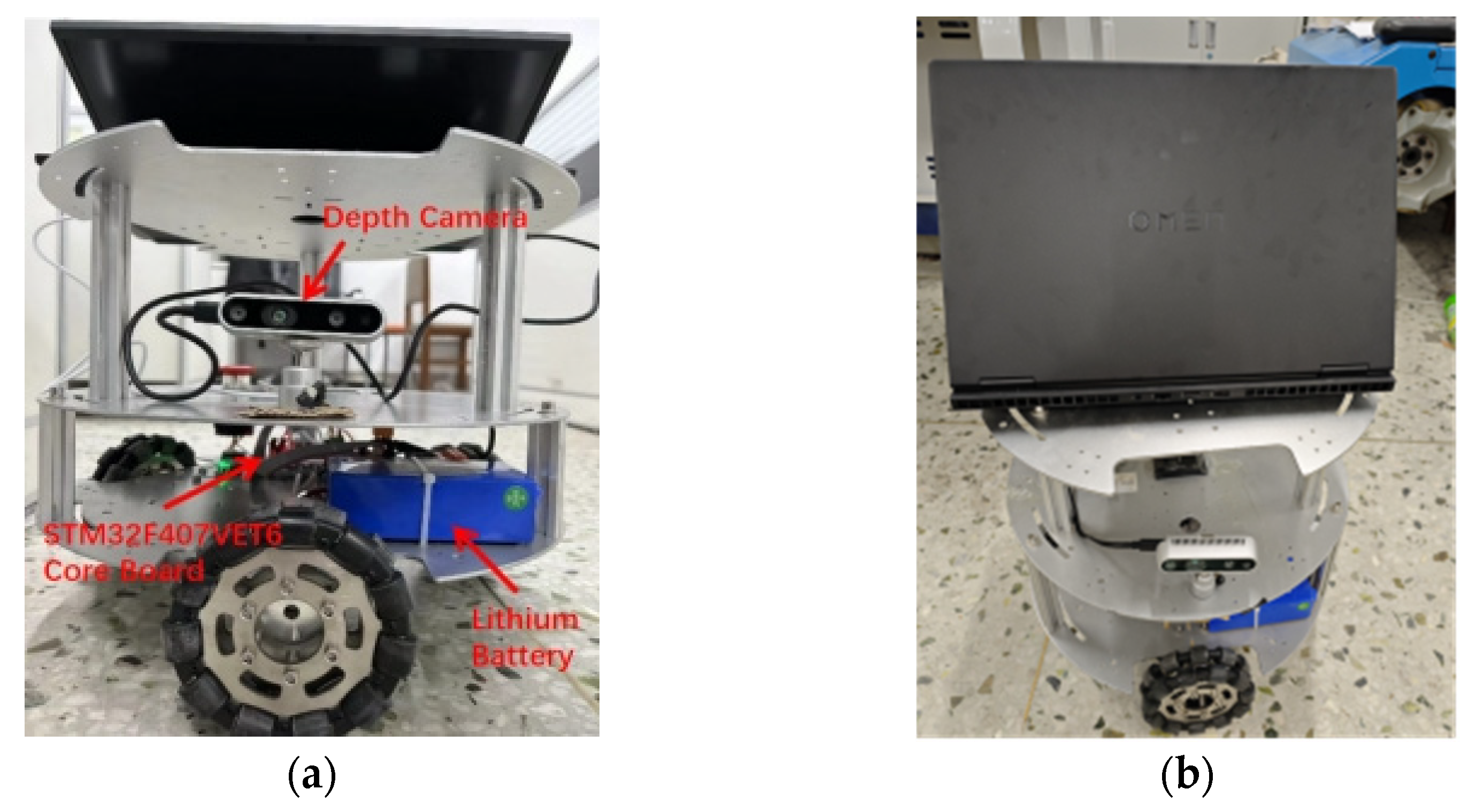
As shown in Figure 1, the three-wheel omnidirectional mobile robot in this study has a radius of 17 cm and a mass of 10 kg, and consists of a top cover module, a control board module, and an omnidirectional chassis. The chassis integrates three N20 DC geared motors (Shenzhen Zhaowei Machinery & Electronics Co., Ltd., Shenzhen, China). The control system is built around an STM32F407VET6 microcontroller (STMicroelectronics, Geneva, Switzerland) running FreeRTOS and integrates motion control, communication, and sensor data processing. Motor closed-loop control is achieved by real-time acquisition of encoder and inertial sensor data.

2.2. Motion Model

2.2.1. Coordinate System

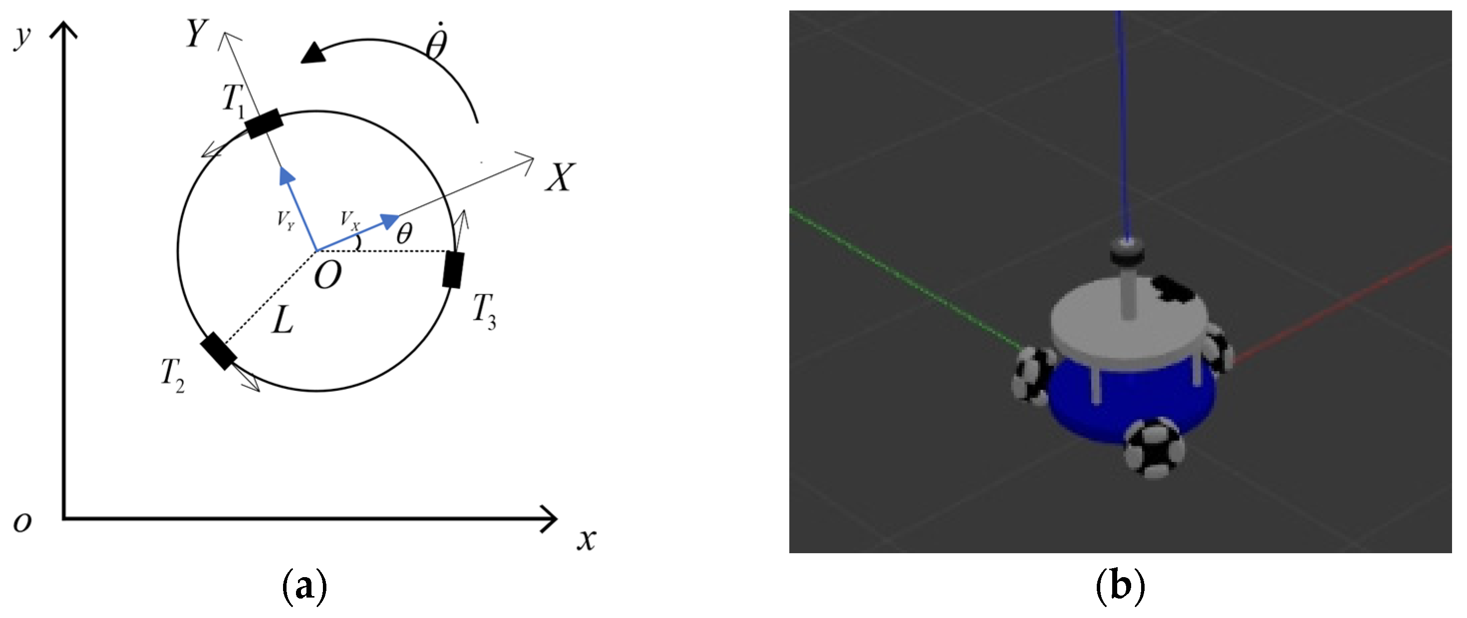
To describe the motion of the mobile robot in the global environment, a global two-dimensional Cartesian coordinate system xoy is first established. Its y-axis points forward and its x-axis points to the right. A robot body coordinate system XOY is further defined with its origin at the geometric center of the chassis to describe the robot’s linear and angular velocities and sensor data and to provide a unified reference for wheel arrangement and kinematic modeling. The overall coordinates of the three-wheel omnidirectional robot are shown in Figure 2.

2.2.2. Kinematic Model

When establishing the kinematic model, the velocities along the y- and x-axes in the global coordinate system are denoted as V_yg and V_xg, and the velocities of the three drive wheels are denoted as V_a, V_b, and V_c. In the robot body coordinate system, the velocities along the Y- and X-axes are denoted as V_yg and V_xg, and the counterclockwise angular velocity is denoted as $\dot{\theta }$. According to the structure of the omnidirectional mobile robot, the center of mass O is located at the geometric center of the chassis and is equidistant from the three drive wheels, denoted as L.

By treating the robot and its wheels as rigid bodies and decomposing the velocities, the kinematic equations of the drive wheels can be expressed as:

$$\left[\begin{array}{c}{V}_a\\ V_b\\ V_c\end{array}\right]=\left[\begin{array}{ccc}-1& 0& L\\ \cos \phi & -\sin \phi & L\\ \cos \phi & \sin \phi & L\end{array}\right]\left[\begin{array}{c}{V}_{xb}\\ V_{yb}\\ \dot{\theta }\end{array}\right]$$

(1)

The global coordinate system serves as a fixed reference to describe the overall pose of the robot in the environment, while the body coordinate system is attached to the robot and moves with it. To accurately represent the robot’s pose in the global coordinate system and convert motion quantities between the two systems, a coordinate transformation relationship is established. The rotation matrix from the body coordinate system to the global coordinate system is defined as:

$$R{=}_B^{G}R=\left[\begin{array}{ccc}\cos \theta & -\sin \theta & 0\\ \sin \theta & \cos \theta & 0\\ 0& 0& 1\end{array}\right]$$

(2)

The velocity and angular velocity vectors in the global and body coordinate systems can be converted as follows:

$$\left[\begin{array}{c}{V}_{xg}\\ V_{yg}\\ \dot{\theta }\end{array}\right]=\left[\begin{array}{ccc}\cos \theta & -\sin \theta & 0\\ \sin \theta & \cos \theta & 0\\ 0& 0& 1\end{array}\right]\left[\begin{array}{c}{V}_{xb}\\ V_{yb}\\ \dot{\theta }\end{array}\right]$$

(3)

By combining Equations (1) and (3):

$$\left[\begin{array}{c}{V}_a\\ V_b\\ V_c\end{array}\right]=\left[\begin{array}{ccc}-\cos \theta & -\sin \theta & L\\ \cos \phi \cos \theta +\sin \phi \sin \theta & \cos \phi \sin \theta -\sin \phi \cos \theta & L\\ \cos \phi \cos \theta -\sin \phi \sin \theta & \cos \phi \sin \theta +\sin \phi \cos \theta & L\end{array}\right]\left[\begin{array}{c}{V}_{xg}\\ V_{yg}\\ {\dot{\theta }}_r\end{array}\right]$$

(4)

Equation (4) represents the kinematic model of the robot discussed in this study, where $\phi ={60}^{°},\hspace{1em}{\left[\begin{array}{ccc}{V}_{xg}& V_{yg}& \dot{\theta }\end{array}\right]}^{\mathrm{T}}$ are the velocities of the y- and x-axes in the global coordinate system and the angular velocity, and V_a, V_b, and V_c are the individual rotational speeds of the three drive wheels.

2.3. Overall Framework of Mobile Robot Path Planning

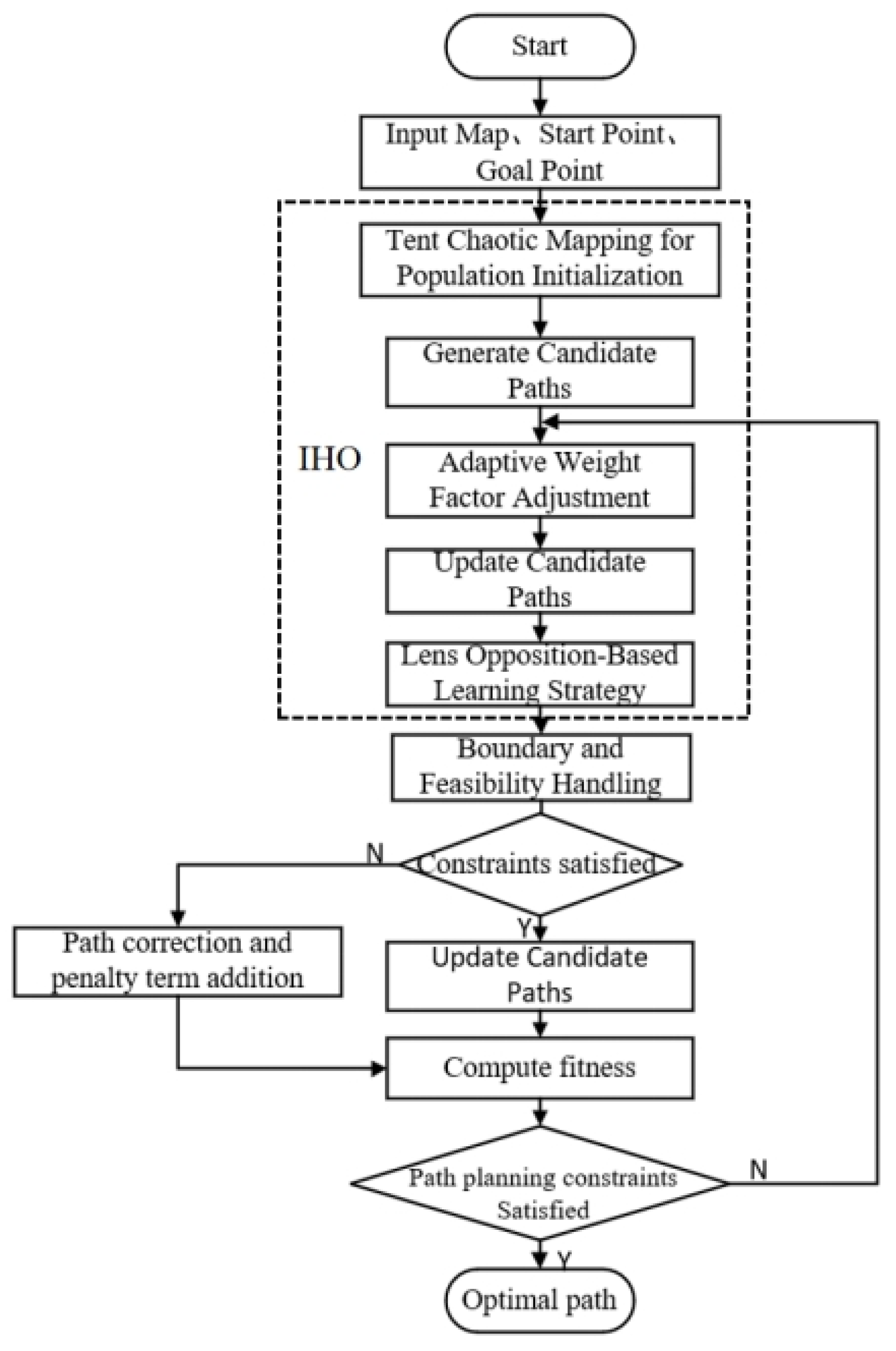
Figure 3 shows the overall framework of mobile robot path planning. The robot first acquires obstacle information through environment perception and constructs a two-dimensional grid map. The path is then represented as a candidate solution consisting of a start point, intermediate waypoints, and a goal point. The improved hippopotamus optimization algorithm is used to search and optimize the path, and the final output is an optimal path that satisfies obstacle avoidance constraints and guides the robot’s motion execution.

3. Algorithm Improvement

3.1. Hippopotamus Optimization Algorithm

The hippopotamus optimization algorithm simulates individual exploration, defense, and escape behaviors in the environment to create a three-stage dynamic search mechanism that balances global search and local exploitation. It shows high performance in multidimensional complex optimization problems and has strong application potential and research value [18].

3.1.1. Random Initialization of the Hippopotamus Population

In the initial stage, the algorithm generates random initial solutions as follows:

$$\begin{array}{l}{X}_i:x_{ij}=l{b}_j+rand\left(0,1\right)\cdot \left(u{b}_j-l{b}_j\right)\hspace{0.33em}\\ (i=1,2,\dots ,N,\hspace{0.33em}j=1,2,\dots ,m)\end{array}$$

(5)

where X_i represents the position of the i-th hippopotamus in each decision variable. ub_j and lb_j are the lower and upper bounds of the j-th decision variable. N is the number of individuals, and m is the number of decision variables in the problem.

In mobile robot path planning, the position vector X_i of the i-th individual represents a candidate path, where its dimension D corresponds to the number of key waypoints in the path, and X_i is defined as follows:

$$X_i=\left(x_{i,1},y_{i,1},x_{i,2},y_{i,2},\dots ,x_{i,D},y_{i,D}\right)$$

(6)

3.1.2. Hippopotamus Position Update in Rivers or Ponds (Exploration Phase)

The algorithm identifies and updates the superior individuals by iteratively evaluating the objective function. The position of the dominant male hippopotamus $X_i^{Mhippo}$ in the population is as follows:

$$\begin{array}{c}{x}_{ij}^{Mhippo}=x_{ij}+y_1\cdot \left(D_{hippo}-I_1\cdot x_{ij}\right)\\ \left(for\hspace{0.33em}i=1,2,\dots ,{\displaystyle \frac{N}{2}}\hspace{0.33em}and\hspace{0.33em}j=1,2,\dots ,m\right)\end{array}$$

(7)

where y₁ is a random number between 0 and 1, I₁ takes the value 1 or 2, and D_hippo represents the position of the dominant hippopotamus, which in the path planning problem corresponds to the candidate path with the lowest cost in the current iteration, meaning a shorter length and better obstacle avoidance performance.

The position of a female or immature hippopotamus $X_i^{F\hspace{0.33em}Bhippo}$ is given by:

$$\begin{array}{c}{x}_{ij}^{F\hspace{0.33em}Bhippo}=\left\{\begin{array}{ll}{x}_{ij}+h_1\cdot \left(D_{hippo}-I_2\cdot M{G}_i\right),\hfill & T>0.6\hfill \\ \equiv \hfill & else\hfill \end{array}\right.\\ \equiv \left\{\begin{array}{ll}{x}_{ij}+h_2\cdot \left(M{G}_i-D_{hippo}\right),\hfill & rand\left(0,1\right)>0.6\hfill \\ l{b}_j+rand\left(0,1\right)\cdot \left(u{b}_j-l{b}_j\right)\hfill & else\hfill \end{array}\right.\hfill \\ \hspace{1em}\hspace{1em}\hspace{1em}(for\hspace{0.33em}i=1,2,\dots ,{\displaystyle \frac{N}{2}}\hspace{0.33em}and\hspace{0.33em}j=1,2,\dots ,m)\hfill \end{array}$$

(8)

where h₁ and h₂ are random scaling coefficients; MG_i is the average position of randomly selected hippopotamuses in the population. In $T=\exp \left(-{\displaystyle \frac{t}{\tau }}\right)$, t is the current iteration number, and τ is the maximum number of iterations. If $rand\left(0,1\right)>0.6$, the position is updated based on the distance between the average and the best individual; otherwise, a new position is generated randomly.

Equations (9) and (10) describe the position update of hippopotamuses in the population during the exploration phase. The objective function F_i represents the cost, which in the path planning problem corresponds to the length of the i-th candidate path.

$$X_i=\left\{\begin{array}{ll}{X}_i^{Mhippo}\hfill & ,F_i^{Mhippo}<F_i\hfill \\ X_i\hfill & ,else\hfill \end{array}\right.$$

(9)

$$X_i=\left\{\begin{array}{ll}{X}_i^{F\hspace{0.33em}Bhippo}\hfill & ,X_i^{F\hspace{0.33em}Bhippo}<F_i\hfill \\ X_i\hfill & ,else\hfill \end{array}\right.$$

(10)

3.1.3. Hippopotamus Defense Against Predators (Exploration Phase)

When the hippopotamus population faces an external threat, its defensive behavior is expressed as a rapid response and directed movement toward the threat. The position of the predator in space is given by:

$$\begin{array}{c}Predato{r}_j=l{b}_j+\overrightarrow{r_8}\cdot \left(u{b}_j-l{b}_j\right)\\ j=1,2,\dots ,m\end{array}$$

(11)

where $\overrightarrow{r_8}$ represents a random vector with values between 0 and 1.

$$\overrightarrow{D}=\left|Predato{r}_j-x_{ij}\right|$$

(12)

$\overrightarrow{D}$ represents the distance between the i-th hippopotamus and the predator. When $F_{\mathrm{Pr}\mathrm{edatorj}}<F_i$, the hippopotamus quickly turns toward the predator and moves to drive it away; when $F_{\mathrm{Pr}\mathrm{edatorj}}>F_i$, the hippopotamus also turns toward the predator, but its movement range is limited.

$$\begin{array}{c}{X}_i^{HippoR}:x_{ij}^{HippoR}=\left\{\begin{array}{ll}\overrightarrow{RL}+Predato{r}_j+\left({\displaystyle \frac{f}{c-d\times \cos (2\pi g)}}\right)\cdot \left({\displaystyle \frac{1}{\overrightarrow{D}}}\right),\hfill & F_{Predato{r}_j}<F_i\hfill \\ \overrightarrow{RL}+Predato{r}_j+\left({\displaystyle \frac{f}{c-d\times \cos (2\pi g)}}\right)\cdot \left({\displaystyle \frac{1}{2\times \overrightarrow{D}+\overrightarrow{r_9}}}\right),\hfill & F_{Predato{r}_j}>F_i\hfill \end{array}\right.\\ \hspace{1em}\hspace{1em}\hspace{1em}\hspace{1em}\hspace{1em}\hspace{1em}\hspace{1em} (for\hspace{0.33em}i=⌈{\displaystyle \frac{N}{2}}⌉+1,⌈{\displaystyle \frac{N}{2}}⌉+2,\dots ,N,\hspace{0.33em}j=1,2,\dots ,m)\hfill \end{array}$$

(13)

The position $X_i^{HippoR}$ of a hippopotamus facing a predator is given by Equation (13), where f, c, d and g are randomly drawn coefficients from a uniform distribution; $\overrightarrow{r_9}$ is a random vector of dimension 1 × m. $\overrightarrow{RL}$ is a random vector following a Lévy distribution used to introduce sudden changes in the predator’s position during an attack. The mathematical model of the random Lévy motion is calculated as follows:

$$Levy(\vartheta )=0.05\times {\displaystyle \frac{w\times {\sigma }_w}{|v{|}^{\frac{1}{\beta }}}}$$

(14)

where w and v are random numbers in the interval [0, 1], $\vartheta$ is a constant (typically 1.5), and ${\sigma }_w$ is calculated as follows:

$${\sigma }_w={\left[{\displaystyle \frac{\Gamma (1+\vartheta )\sin \left(\frac{\tau -\vartheta }{2}\right)}{\Gamma \left(\frac{1+\vartheta }{2}\right)\vartheta 2^{\frac{\tau -2}{2}}}}\right]}^{{\displaystyle \frac{1}{\vartheta }}}$$

(15)

where $\Gamma$ denotes the Gamma function.

The position of a hippopotamus in the population when facing a predator is updated as follows:

$$X_i=\left\{\begin{array}{ll}{X}_i^{HippoR}\hfill & ,F_i^{HippoR}<F_i\hfill \\ X_i\hfill & ,F_i^{HippoR}\ge F_i\hfill \end{array}\right.$$

(16)

When $F_i^{HippoR}<F_i$, the predator flees and the hippopotamus remains in the population. When $F_i^{HippoR}\ge F_i$, the hippopotamus is captured, and another individual replaces it in the herd.

3.1.4. Hippopotamus Escaping from the Predator (Exploitation Phase)

When a hippopotamus cannot drive away the predator with defensive behavior, it adopts an escape strategy to find a safe position. Its random escape position $X_i^{HippoE}$ is calculated as follows:

$$\begin{array}{c}{x}_{ij}^{\mathit{HippoE}}=x_{ij}+r_{10}·\left(l{b}_j^{\mathit{local}}+s_1·\left(u{b}_j^{\mathit{local}}-l{b}_j^{\mathit{local}}\right)\right)\\ \hspace{1em}\hspace{1em}\hspace{1em} (i=1,2,\dots ,N,j=1,2,\dots ,m)\hfill \end{array}$$

(17)

where $l{b}_j^{local}={\displaystyle \frac{l{b}_j}{t}},\hspace{0.33em}u{b}_j^{local}={\displaystyle \frac{u{b}_j}{t}}$ represent the adaptive local lower and upper bounds of the hippopotamus position, and t is the current iteration number.

The position of a hippopotamus during escape is updated as follows:

$$X_i=\left\{\begin{array}{ll}{X}_i^{HippoE}\hfill & ,\hspace{0.33em}{F}_i^{HippoE}<F_i\hfill \\ X_i\hfill & ,\hspace{0.33em}{F}_i^{HippoE}\ge F_i\hfill \end{array}\right.$$

(18)

When $F_i^{HippoE}<F_i$, the hippopotamus has found a safer position near its current location.

3.2. Improved Hippopotamus Optimization Algorithm

Recent studies have proposed several improvement strategies for the hippopotamus optimization (HO) algorithm, such as SPM chaotic mapping, cubic chaotic mapping, mutation operators, tangent flight strategies, and other hybrid search mechanisms. These methods can improve algorithm performance in specific optimization problems. However, some of them have complex structures and require more parameters. If they are directly applied to mobile robot path planning, they may increase implementation difficulty and computational cost.

The method proposed in this paper focuses on the functional matching between the improvement strategies and the original three-stage search mechanism of HO. Therefore, this study selects strategies that are widely used, structurally clear, and easy to embed into the original HO framework. Tent chaotic mapping is used to improve the uniformity of the initial population distribution. The exponential nonlinear adaptive weight factor is used to adjust the balance between early global exploration and later local exploitation. The lens opposition-based learning strategy is used to improve the ability of the algorithm to escape local optima during the local search stage. These strategies keep the algorithm structure relatively simple while improving search accuracy, stability, and engineering applicability.

3.2.1. Tent Chaotic Mapping

High diversity in the initial population helps to improve global search efficiency and convergence accuracy [24]. Chaotic mapping is used as a random operator, and its uniform traversal property can increase population diversity. For the hippopotamus optimization algorithm, the spatial coverage of the initial population directly affects the search performance of the first stage, namely position update in rivers or ponds. If the initial individuals are too concentrated in a local region, the algorithm may have an insufficient search range in the early stage and may become trapped in a local region. Therefore, introducing chaotic mapping during the initialization stage of HO can improve the uniformity of individual distribution and strengthen early global exploration.

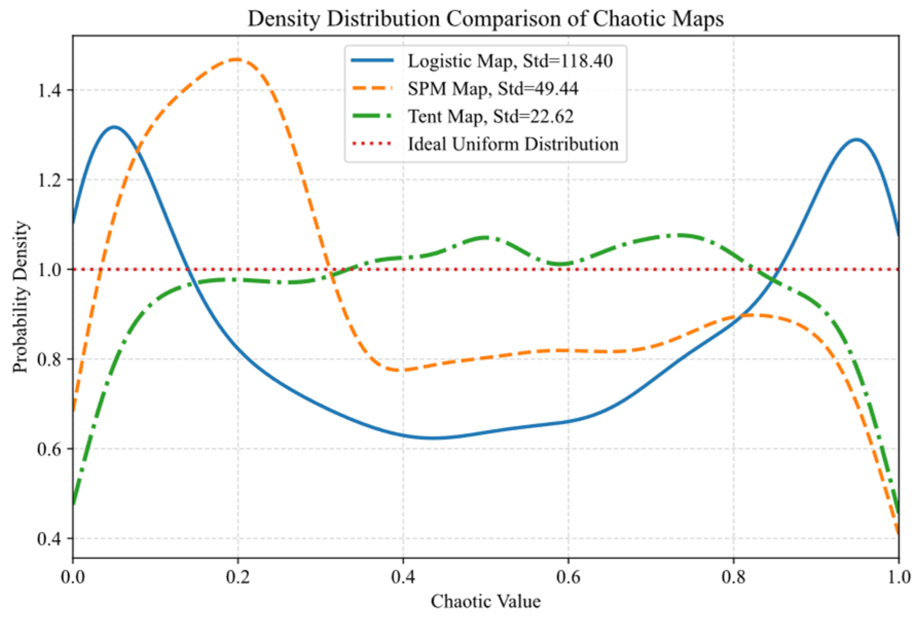
Common chaotic maps include Logistic mapping, SPM mapping, and Tent mapping. To compare the initialization distribution characteristics of different chaotic maps, this study uses kernel density estimation to analyze the probability density distributions of the Logistic, SPM, and Tent chaotic sequences in the interval [0, 1].

As shown in Figure 4, Logistic mapping has clear density peaks near the two ends of the interval, while the density in the middle region is lower. This indicates boundary clustering and insufficient coverage in the central region. SPM mapping shows large peaks in some local intervals. This suggests that it has strong perturbation ability, but its distribution fluctuates greatly and its uniformity is still limited. In contrast, the probability density curve of Tent mapping is flatter and closer to the ideal uniform distribution reference line. Also, Tent mapping has the smallest frequency standard deviation, which further shows that the sequence generated by Tent mapping has better uniform traversal characteristics in the interval.

From the search mechanism of HO, the first stage performs global exploration based on the relationships among the position of the dominant hippopotamus, the mean position of randomly selected individuals, and the current population positions. The uniform initial population generated by Tent mapping can improve the spatial representativeness of the dominant individual and the population mean. This allows the hippopotamus population to obtain more sufficient search directions in the initial stage and achieve faster traversal and information coverage in the search space, which improves the optimization speed and search efficiency of the algorithm [25]. Also, Tent mapping is only used in the initialization stage and does not change the three-stage search structure of HO, so it has good compatibility with the original HO algorithm. Therefore, Tent chaotic mapping is used to initialize the hippopotamus population in this study, and its formula is given as follows:

$$x_{k+1}=\left\{\begin{array}{ll}{\displaystyle \frac{x_k}{\mu }}\hfill & ,\hspace{0.33em}{x}_k<\mu \hfill \\ {\displaystyle \frac{1-x_k}{1-\mu }}\hfill & ,\hspace{0.33em}{x}_k>\mu \hfill \end{array}\right.$$

(19)

The control parameter μ of Tent mapping determines the segmentation ratio of the mapping interval. When μ deviates from 0.5, the stretching degrees on the two sides of the interval are not consistent, and the chaotic sequence may show distribution bias in some regions. When μ = 0.5, the two segments of Tent mapping have a symmetric structure, and the sequence shows stronger traversal ability and a more uniform distribution in the interval [0, 1]. Therefore, μ = 0.5 is used as the Tent chaotic mapping parameter in this study to obtain a more uniform initial population distribution.

The population initialization formula with Tent chaotic mapping is given as follows:

$$\begin{array}{l}{X}_{i:j}=l{b}_j+chaos\cdot (u{b}_j-l{b}_j)\hspace{0.33em}\\ (i=1,2,\dots ,N,j=1,2,\dots ,m)\end{array}$$

(20)

where chaos is a two-dimensional chaotic sequence matrix generated by Tent mapping with size [N, m].

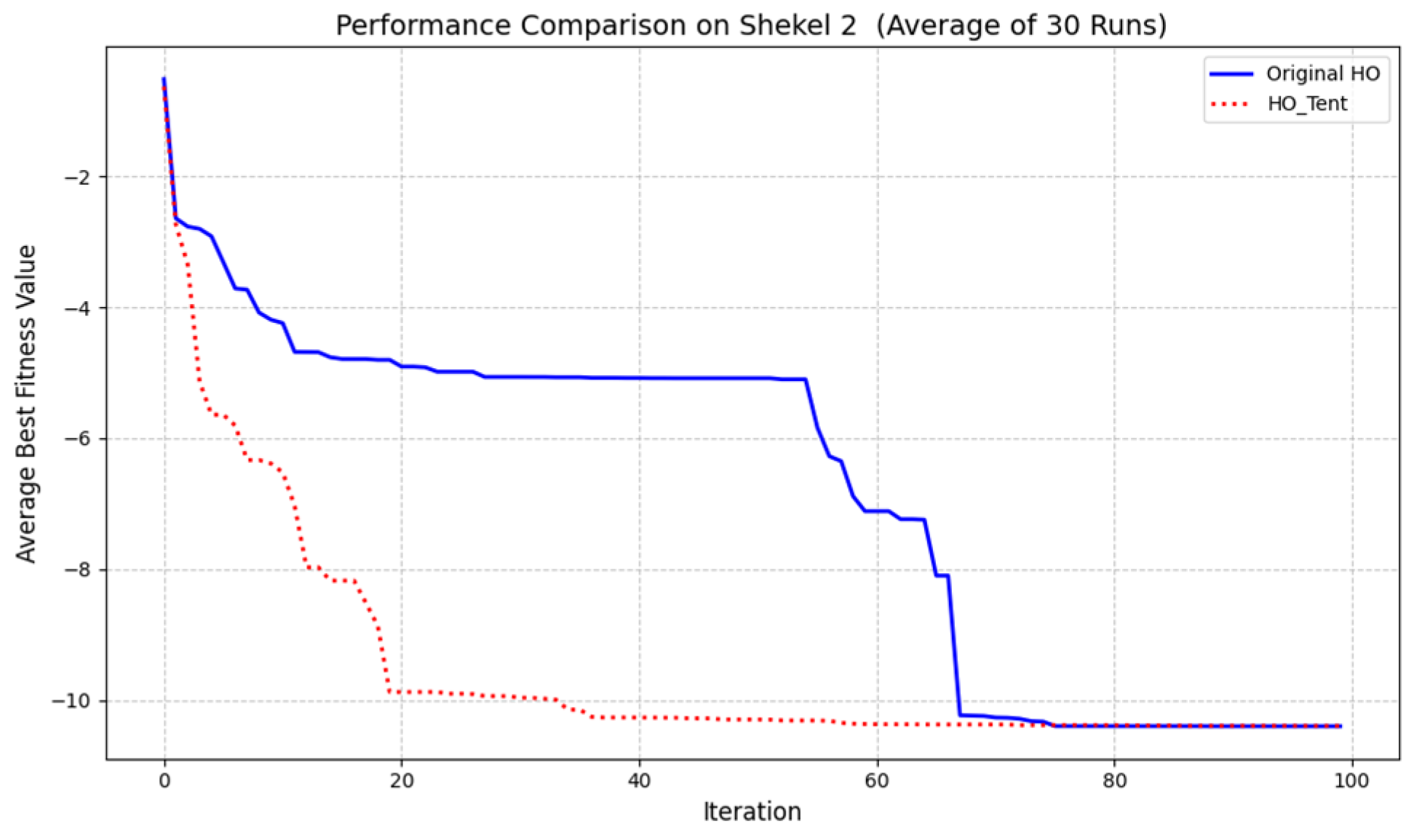
Experiments were conducted on the benchmark function set using the hippopotamus optimization algorithm with Tent chaotic mapping. The Shekel 2 function is taken as an example, and the results are shown in Figure 5.

As shown in the figure, the improved algorithm (HO_Tent) shows better optimization performance than the original algorithm. In the early stage, the chaotic sequence generated by the Tent mapping makes the initial population more uniformly distributed in the search space, which increases population diversity and strengthens global exploration, leading to faster convergence and stronger global optimization ability.

3.2.2. Adaptive Weight Factor

To meet the different search requirements of the hippopotamus optimization algorithm at different iteration stages, this study introduces a nonlinear adaptive weight factor to regulate the individual position update process. Compared with a linearly decreasing weight, the exponential weight does not decrease at a constant rate. Instead, its decreasing speed at different iteration stages can be controlled by the tuning coefficient. This allows the algorithm to maintain stronger global search ability in the early stage and achieve clearer search contraction in the later stage. Compared with a cosine-based weight, the exponential weight has a simpler structure and can directly control the transition speed from exploration to exploitation through the exponential term. Therefore, an exponential nonlinear adaptive weight factor is introduced during the position update of the hippopotamus population in this study. The weight coefficient w(t) is defined as follows:

$$w(t)=e^{-{\left({\displaystyle \frac{t}{\max \_iter}}\right)}^k}$$

(21)

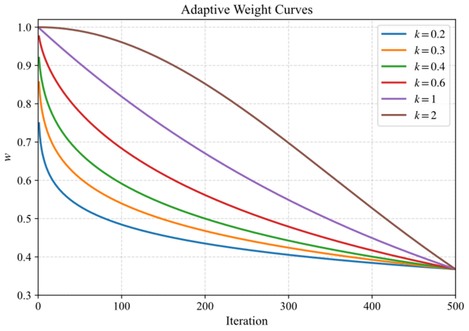
where t is the current iteration number, max_iter is the maximum number of iterations, and k is a tuning coefficient. The weight variation curves under different values of k are shown in Figure 6.

A larger k leads to a slower decrease in the weight factor in the early stage and a faster decrease in the later stage [26]. When $t<{\displaystyle \frac{\max \_iter}{2}}$, the algorithm has a large weight in the early iterations, k is set to 2, the weight decreases slowly and the algorithm maintains strong global search ability. As the number of iterations increases, when $t\ge {\displaystyle \frac{\max \_iter}{2}}$, the search radius decreases, the algorithm performs more precise search in a local region, k is set to 0.2, the weight decreases faster and the local exploitation ability of the algorithm is enhanced. The weight factor w(t) is defined as follows:

$$w(t)=e^{-{\left({\displaystyle \frac{t}{\max \_iter}}-0.5\right)}^k}$$

(22)

The proposed piecewise exponential nonlinear weight function allows the algorithm to maintain strong exploration ability in the early stage and quickly contract the search range in the later stage. This better matches the search requirements of HO at different stages.

By incorporating the adaptive weight factor into the hippopotamus position update, Formulas (7) and (13) become:

$$\begin{array}{c}{X}_i^{Mhippo}:x_{ij}^{Mhippo}=w(t)\times x_{ij}+y_1\cdot \left(D_{hippo}-I_1\cdot x_{ij}\right)\\ (for\hspace{0.33em}i=1,2,\dots ,{\displaystyle \frac{N}{2}}\hspace{0.33em}and\hspace{0.33em}j=1,2,\dots ,m)\end{array}$$

(23)

$$\begin{array}{c}{X}_i^{HippoR}:x_{ij}^{HippoR}=\left\{\begin{array}{ll}w(t)\times \overrightarrow{R}L+Predato{r}_j+\left({\displaystyle \frac{f}{(c-d\times \cos (2\pi g))}}\right)\cdot \left({\displaystyle \frac{1}{D}}\right)\hfill & ,\hspace{0.33em}{F}_{Predatorj}<F_i\hfill \\ w(t)\times \overrightarrow{R}L+Predato{r}_j+\left({\displaystyle \frac{f}{(c-d\times \cos (2\pi g))}}\right)\cdot \left({\displaystyle \frac{1}{2\times \overrightarrow{D}+{\overrightarrow{r}}_9}}\right)\hfill & ,\hspace{0.33em}{F}_{Predatorj}>F_i\hfill \end{array}\right.\\ \hspace{1em}\hspace{1em}\hspace{1em}\hspace{1em}\hspace{1em}\hspace{1em}\hspace{1em}\hspace{1em}\hspace{1em}(for\hspace{0.33em}i=⌊{\displaystyle \frac{N}{2}}⌋+1,⌊{\displaystyle \frac{N}{2}}⌋+2,\dots ,N,j=1,2,\dots ,m)\hfill \end{array}$$

(24)

Since the third stage of the algorithm involves local contraction, introducing the weight factor there may cause overly fast convergence and weaken local search ability. Therefore, the adaptive weight factor is applied only in the first and second stages of the position update.

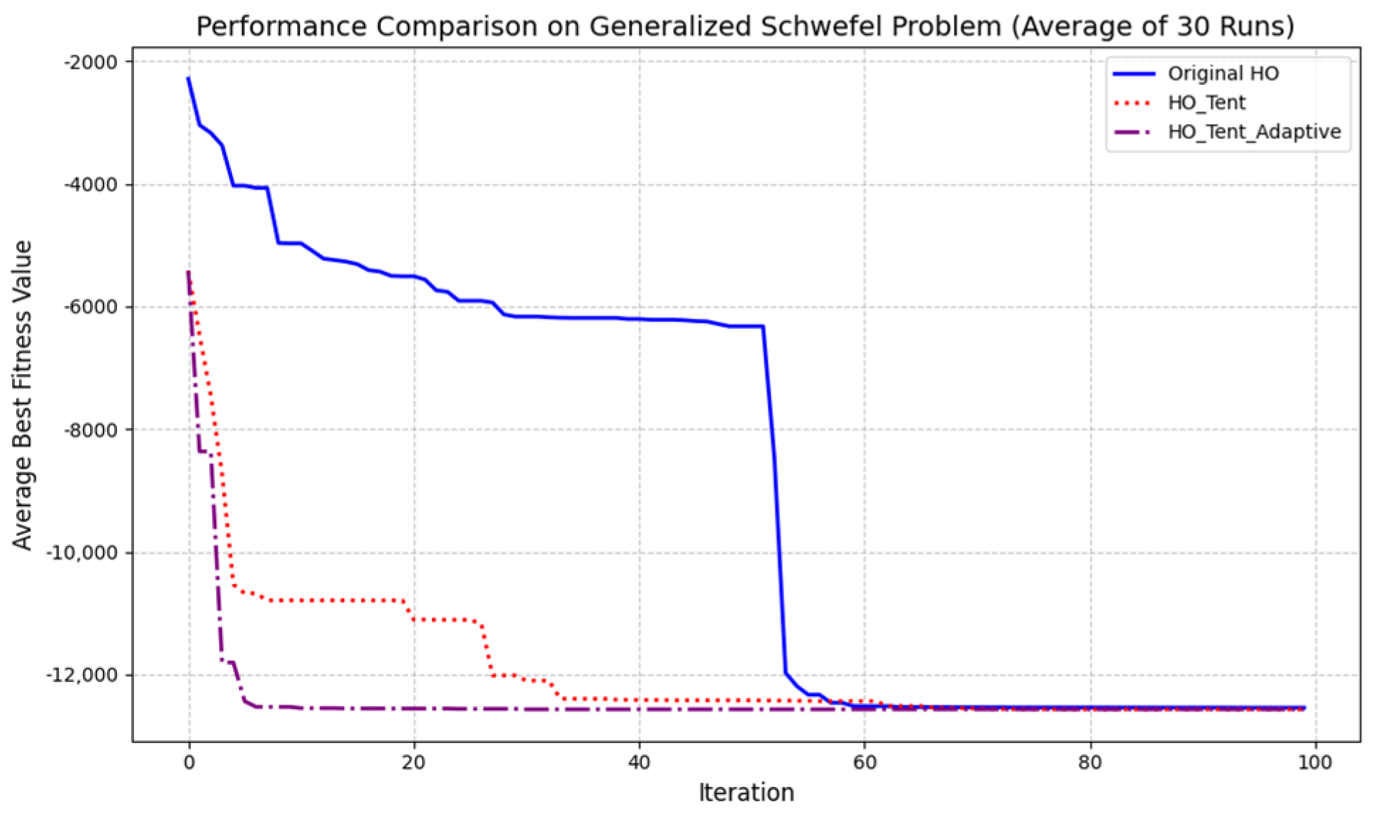
Experiments were conducted on the benchmark function set using the hippopotamus algorithm integrating Tent chaotic mapping and the adaptive weight factor. The Generalized Schwefel’s Problem function is taken as an example, and the results are shown in Figure 7.

As shown in the figure, the hippopotamus algorithm with Tent chaotic mapping and an adaptive weight factor (HO_Tent_Adaptive) decreases more rapidly in the early iterations, demonstrating stronger global search ability and quickly locating high-quality solution regions. In the middle and later iterations, the curve stabilizes and the final convergence value is lower, indicating higher local exploitation accuracy and better convergence stability in the later stage.

3.2.3. Lens Opposition-Based Learning Strategy

The lens opposition-based learning strategy (LOBL) combines opposition-based learning with lens imaging principles to enhance the global search ability and overall performance of the algorithm. During optimization, LOBL generates an opposite solution to the current candidate solution through lens mapping, and the better of the two is selected as the initial solution for the next iteration [27]. The formula is as follows:

$$x_j^{*}={\displaystyle \frac{u{b}_j+l{b}_j}{2}}+{\displaystyle \frac{u{b}_j+l{b}_j}{2m}}-{\displaystyle \frac{x_j}{m}}$$

(25)

where ub_j and lb_j represent the lower and upper bounds of the j-th decision variable, and m is the lens factor. When m > 1, the opposite solution is closer to the midpoint, favoring local exploitation; when m < 1, the opposite solution is farther from the midpoint, helping to escape local optima. Tent chaotic mapping and the adaptive weight factor enhance the global exploration ability of the algorithm in the early stage, while the third stage of the original hippopotamus optimization algorithm should further strengthen local exploitation. To determine a reasonable value of the lens factor, this study selects m = 1.0, 1.5, 2.0, and 2.5 for parameter sensitivity analysis. The Kowalik test function is used as an example for comparison. The algorithm performance under different values of $m$ is evaluated using the best value, worst value, standard deviation, and average iteration to best. The results are shown in

Table 1. Sensitivity analysis results under different lens factor m values.

m	Best	Worst	Std	Average Iteration to Best
1.0	−10.4079	−10.3773	0.0096	87.9
1.5	−10.4079	−10.3452	0.0069	81.1
2.0	−10.4079	−10.3727	0.0087	83.3
2.5	−10.4081	−10.3920	0.0041	85.5

.

As shown in Table 1, the algorithm obtains good optimization results under different values of the lens factor m. This indicates that the lens opposition-based learning strategy has a certain robustness to parameter changes. Compared with the other values, m = 1.5 maintains good optimization accuracy and shows faster convergence, allowing the algorithm to reach a better solution within fewer iterations. Based on optimization accuracy, stability, and convergence efficiency, m = 1.5 is selected as the parameter of the lens opposition-based learning strategy in this study. This setting provides moderate perturbation for the opposite solution and favors local exploitation, which helps the algorithm escape local optima while avoiding excessive random disturbance to convergence stability.

In the third stage of the hippopotamus optimization algorithm, the opposite solution $X_i^{opposite}$ to the current candidate solution is generated and compared with the candidate solution for position updating, as follows:

$$X_i=\left\{\begin{array}{ll}{X}_i^{opposite}\hfill & ,\hspace{0.33em}{F}_i^{opposite}<F_i\hfill \\ X_i\hfill & ,\hspace{0.33em}{F}_i^{opposite}\ge F_i\hfill \end{array}\right.$$

(26)

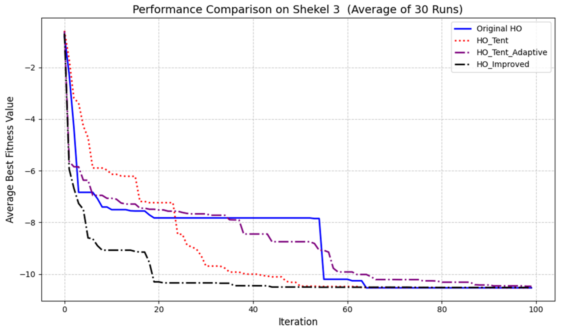
Experiments were conducted on the benchmark function set using the hippopotamus algorithm integrating Tent chaotic mapping, an adaptive weight factor, and the lens opposition-based learning strategy. The Shekel 3 function is taken as an example, and the results are shown in Figure 8.

As shown in the figure, the hippopotamus algorithm with the lens opposition-based learning strategy demonstrates significantly better overall optimization performance than the other algorithms. In the early iterations, it approaches the global optimum region more quickly, showing higher convergence speed; in the middle and later iterations, it maintains a stable optimization trend and can rapidly escape local optima, further improving search accuracy and stability.

3.3. Algorithm Runtime Analysis

The three improvement strategies improve the search performance of the algorithm, but they also introduce additional computational cost. To further analyze the effect of different improvement strategies on runtime efficiency, this study compares the runtime of the original HO, HO_Tent, HO_Tent_Adaptive, and the final IHO. To quantitatively evaluate the effect of these strategies on algorithm efficiency, unimodal, multimodal, and fixed-dimension multimodal functions are selected as test functions. Under the same experimental conditions, the average runtime of different algorithms is recorded. Each algorithm is run independently 30 times on each test function, and the best value, standard deviation, and average runtime are recorded. The results are shown in

Table 2. Runtime comparison of different improvement strategies on benchmark functions.

Function Category	Algorithms	Best	Std	Average Runtime/s
Unimodal Benchmark Functions Sphere	HO	8.77 × 10−75	2.15 × 10−72	0.1032
	HO_Tent	2.03 × 10−76	7.61 × 10−69	0.1007
	HO_Tent_Adaptive	4.97 × 10−95	2.31 × 1080	0.1055
	IHO	0.00	0.00	0.1882
Multimodal Benchmark Functions Generalized Schwefel’s Problem	HO	−1.25 × 104	9.69	0.0979
	HO_Tent	−1.25 × 104	1.42 × 10	0.0963
	HO_Tent_Adaptive	−1.25 × 104	1.10 × 10	0.1011
	IHO	−1.25 × 104	3.62	0.2019
Fixed-Dimension Multimodal Benchmark Functions Kowalik	HO	−1.05 × 10	2.57 × 10−3	0.1930
	HO_Tent	−1.05 × 10	2.40 × 10−3	0.1898
	HO_Tent_Adaptive	−1.05 × 10	3.74 × 10−3	0.1903
	IHO	−1.05 × 10	5.69 × 10−3	0.8674

.

As shown in Table 2, the average runtime of HO_Tent on the three types of test functions is slightly lower than that of the original HO. This result shows that Tent chaotic mapping adds the generation of chaotic sequences during the initialization stage, but its computational cost is small and has no clear negative effect on the overall runtime efficiency of the algorithm. At the same time, Tent chaotic mapping improves the uniformity of the initial population distribution. This helps the algorithm to obtain better dominant individuals and population search directions in the early stage, which reduces some ineffective search processes.

The runtime of HO_Tent_Adaptive and IHO increases to some extent. However, based on the best fitness values and standard deviations in the table, IHO achieves higher optimization accuracy and better stability on most test functions. Therefore, the additional computational cost of IHO is acceptable because it leads to better search ability and more stable convergence in optimization tasks.

3.4. Flow of the Improved Hippopotamus Optimization Algorithm

In summary, this study improves the original hippopotamus optimization (HO) algorithm by introducing Tent chaotic initialization, a nonlinear adaptive weight factor, and the lens opposition-based learning strategy, forming the improved hippopotamus optimization (IHO) algorithm. The detailed procedure is as follows:

Step 1: Set the population size N, maximum number of iterations T, problem dimension D, and lower and upper bounds UB and LB. Initialize the population using Tent chaotic mapping.

Step 2: Evaluate the fitness of each individual and determine the current global best solution.

Step 3: Update positions in stages 1 and 2 using the nonlinear adaptive weight factor w(t) according to Formulas (23) and (24), and update positions in stage 3 using the opposite solutions of candidates according to Formula (25).

Step 4: Repeat Steps 2–3 until the maximum number of iterations is reached.

Step 5: Output the optimal solution.

4. Benchmark Function Testing and Result Analysis

4.1. Simulation Platform

The experiments were conducted in the following environment: operating system: Windows 11; CPU: Intel Core i9-12900H, 2.50 GHz; memory: 16 GB; and programming environment: Python 3.11.

4.2. Benchmark Function Settings

To comprehensively evaluate the performance of the IHO algorithm, six representative benchmark functions were selected from the test function set and compared with particle swarm optimization (PSO) [28], Bat Algorithm (BA) [29], whale optimization algorithm (WOA) [30], Dragonfly Algorithm (DA) [31], and Harris Hawks Optimization (HHO) [32]. The population size N for all algorithms was set to 16, and the maximum number of iterations was 100. The benchmark functions are listed in

Table 3. Benchmark functions.

Function Category	Benchmark Functions	Value Range	Theoretical Minimum Value
Unimodal Benchmark Functions	$f_1(x)={\displaystyle \sum _{i=1}^n{x}_i^2}$	xi ∈ [−100, 100]	0
	$f_2(x)=\max \left\{\right|x_i|,\hspace{0.33em}1\le i\le D\}$	xi ∈ [−100, 100]	0
Multimodal Benchmark Functions	$f_3(x)={\displaystyle \sum _{i=1}^{30}-}{x}_i\sin \left(\sqrt{\left|x_i\right|}\right)$	xi ∈ [−500, 500]	−12,569.5
	$f_4(x)={\displaystyle \sum _{i=1}^n{x}_i^2}+{\left({\displaystyle \sum _{i=1}^{n}0}.5i{x}_i\right)}^2+{\left({\displaystyle \sum _{i=1}^{n}0}.5i{x}_i\right)}^4$	xi ∈ [−5, 10]	0
Fixed-Dimension Multimodal Benchmark Functions	$f_5(x)={\left({\displaystyle \frac{1}{500}}+{\displaystyle \sum _{j=1}^{25}\frac{1}{j+{\displaystyle \sum _{i=1}^2{\left(x_i-a_{ij}\right)}^6}}}\right)}^{-1}$	xi ∈ [−65, 65]	1
	$f_6(x)=-{\displaystyle \sum _{i=1}^7{\left[(x-a_i){(x-a_i)}^T+c_i\right]}^{-1}}$	xi ∈ [0, 10]	−10.4029

, and the parameter settings of the algorithms are provided in

Table 4. Parameter settings of the algorithms.

Algorithms	Parameter	Value
IHO	Chaotic mapping parameter (μ)	0.5
	Adaptive weight tuning coefficient (k)	2.0 and 0.2
	Lens opposition-based learning factor (m)	1.5
PSO	Inertia weight (w)	0.9
	Cognitive learning factor (c1)	2
	Social learning factor (c2)	2
BA	Loudness attenuation coefficient (α)	0.9
	Pulse emission rate enhancement coefficient ($\gamma$)	0.9
WOA	Spiral parameter (spiral_param)	1
DA	Inertia weight (w)	Linearly decreases from 0.9 to 0.4
	Adaptive coefficient (my_c)	Linearly decreases from 0.1 to 0
HHO	Lévy exponent (β)	1.5
	Escape energy decay factor (e_r_factor)	Linearly decreases from 2 to 0

.

4.3. Benchmark Function Results and Analysis

To ensure the reliability of the results, each comparative algorithm was independently run 30 times on the benchmark functions, and the results are summarized in

Table 5. Results of benchmark functions.

Function	Metric	PSO	BA	WOA	DA	HHO	HO	IHO
f1 (D = 50)	Best	4.49 × 104	8.09 × 104	8.81 × 10−4	1.23 × 105	1.61 × 10−8	2.01 × 10−74	0.00
	Worst	7.41 × 104	9.28 × 104	6.57 × 10−2	1.48 × 105	3.93 × 10−4	1.12 × 10−65	0.00
	Mean	6.27 × 104	8.57 × 104	2.08 × 10−2	1.34 × 105	8.62 × 10−5	2.63 × 10−66	0.00
	Std	1.06 × 104	5.27 × 103	2.53 × 10−2	1.03 × 105	1.54 × 10−4	4.32 × 10−66	0.00
f2 (D = 50)	Best	8.78 × 10	7.39 × 10	4.23 × 10	8.86 × 10	2.50 × 10−3	2.18 × 10−38	4.94 × 10−324
	Worst	9.47 × 10	7.89 × 10	7.18 × 10	9.34 × 10	8.93 × 10	2.88 × 10−36	8.40 × 10−323
	Mean	9.06 × 10	7.63 × 10	6.21 × 10	9.16 × 10	3.96 × 10	7.98 × 10−37	1.98 × 10−323
	Std	2.43	1.90	1.11 × 10	1.70	3.85 × 10	1.11 × 10−36	0.00
f3 (D = 30)	Best	−8.26 × 103	−4.19 × 103	−8.97 × 103	−6.03 × 103	−1.26 × 104	−1.26 × 104	−1.26 × 104
	Worst	−5.89 × 103	−3.39 × 103	−7.61 × 103	−3.06 × 103	−9.01 × 103	−1.25 × 104	−1.26 × 104
	Mean	−7.28 × 103	−3.83 × 103	−8.15 × 103	−4.37 × 103	−1.11 × 104	−1.26 × 104	−1.26 × 104
	Std	7.85 × 102	2.86 × 102	4.52 × 102	1.19 × 103	1.74 × 103	1.39 × 10	4.14
f4 (D = 50)	Best	1.86 × 103	7.86 × 102	1.35 × 103	1.59 × 1010	5.33 × 102	5.63 × 10−76	1.35 × 10−96
	Worst	2.30 × 103	8.19 × 102	1.47 × 103	1.41 × 1011	8.09 × 102	6.87 × 10−70	2.52 × 10−83
	Mean	2.08 × 103	8.02 × 102	1.41 × 103	7.82 × 1010	6.71 × 102	3.44 × 10−70	1.26 × 10−83
	Std	2.21 × 102	1.63 × 10	6.17 × 10	6.23 × 1010	1.38 × 102	3.44 × 10−70	1.26 × 10−83
f5 (D = 2)	Best	9.98 × 10−1	9.98 × 10−1	2.98	9.98 × 10−1	2.98	9.98 × 10−1	9.98 × 10−1
	Worst	1.02	7.87	1.08 × 10	1.55 × 10	1.64 × 10	9.98 × 10−1	9.98 × 10−1
	Mean	1.00	2.97	4.74	5.29	7.23	9.98 × 10−1	9.98 × 10−1
	Std	8.21 × 10−3	2.56	3.04	5.20	5.50	4.01 × 10−10	7.18 × 10−7
f6 (D = 4)	Best	−1.04 × 10	−8.15	−1.04 × 10	−1.04 × 10	−1.04 × 10	−1.04 × 10	−1.04 × 10
	Worst	−2.75	−2.30	−5.22 × 10−1	−5.13	−1.09	−1.04 × 10	−1.04 × 10
	Mean	−5.22	−3.91	−3.94	−7.13	−7.20	−1.04 × 10	−1.04 × 10
	Std	2.80	2.17	3.61	2.45	3.60	2.50 × 10−3	3.67 × 10−3

.

The comparative results indicate that for unimodal benchmark functions, the IHO algorithm achieves better results than all other algorithms in terms of best value, worst value, mean, and standard deviation. For multimodal benchmark functions, IHO produces results closer to the theoretical optimum with lower standard deviation. For fixed-dimension multimodal benchmark functions, IHO also achieves results nearer to the theoretical optimum with smaller standard deviation than most comparative algorithms, demonstrating superior stability and accuracy.

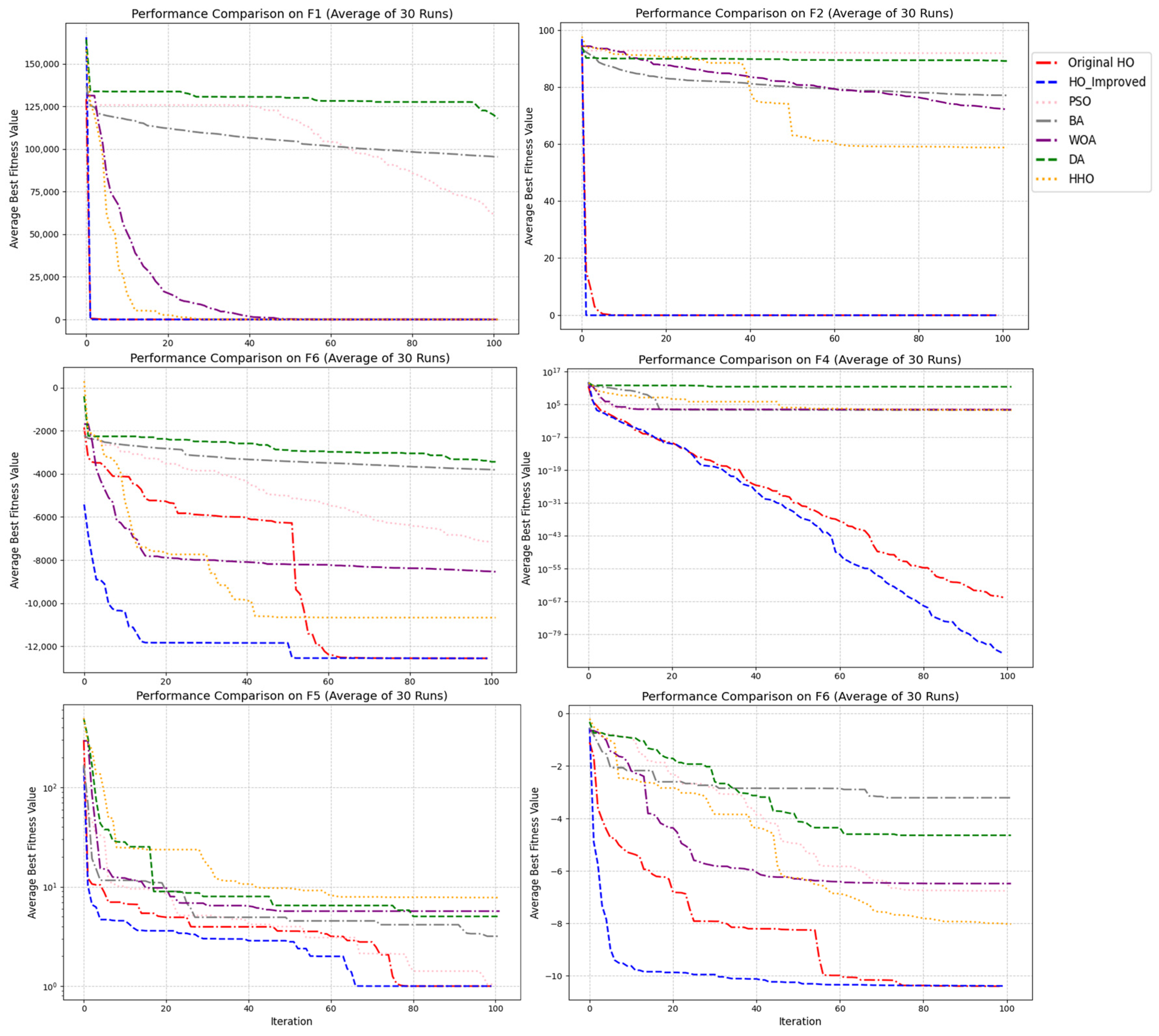
Figure 9 shows the optimization convergence curves of the IHO algorithm and the comparative algorithms on the benchmark functions. The curves are plotted based on the average best fitness value at each iteration over 30 independent runs, objectively reflecting the overall convergence behavior and stability of each algorithm.

The IHO and HO algorithms both show fast convergence on unimodal functions, with their final results being similar, indicating strong global search ability on low-complexity problems. For multimodal functions, IHO reduces the fitness value more quickly in the early iterations and converges steadily later, effectively avoiding local optima. In some tests, both IHO and HO continue to converge while other algorithms stagnate in local optima, and IHO converges faster in the later iterations. Overall, IHO outperforms the comparative algorithms on multimodal functions, showing rapid early convergence and maintaining strong search activity later, demonstrating robust global optimization capability and stable convergence performance.

The experimental results show that the IHO algorithm achieves high solution accuracy, fast convergence, and strong stability across all types of benchmark functions, confirming its ability to balance global exploration and local exploitation in complex optimization problems, effectively avoid premature convergence, and demonstrate robust optimization performance and reliability.

5. Global Path Planning Experimental Results and Analysis

5.1. Experimental Setup

5.1.1. Grid Map Environment Modeling

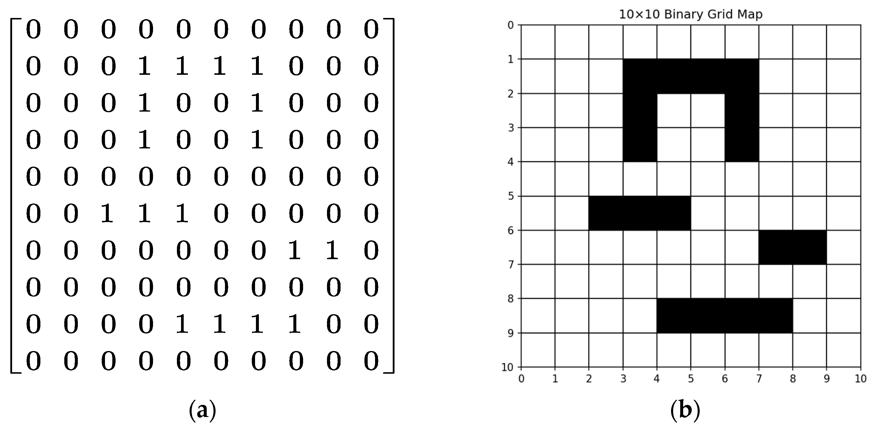
This study uses a two-dimensional grid map to model the mobile robot working environment and perform path planning [33]. For the real environment map, grayscale and binarization processing are first applied, and the map is stored in the form of a two-dimensional matrix, where “1” represents obstacle regions and “0” represents traversable areas, as shown in Figure 10.

5.1.2. Locomotion Mode

In this study, the Euclidean step length is used to calculate the path length in the two-dimensional grid map. The path consists of a sequence of connected grid nodes P = {P₀, P₁, P₂⋯P_n}, where P_i = (x_i, y_i) represents the coordinate of the i-th grid node, and the step length between adjacent nodes is defined by the Euclidean distance as follows:

$$d(p_i,p_{i+1})=\sqrt{{(x_{i+1}-x_i)}^2+{(y_{i+1}-y_i)}^2}$$

(27)

The total path length is calculated as the sum of all step lengths as follows:

$$L(P)={\displaystyle \sum _{i=0}^{n-1}d}(p_i,p_{i+1})$$

(28)

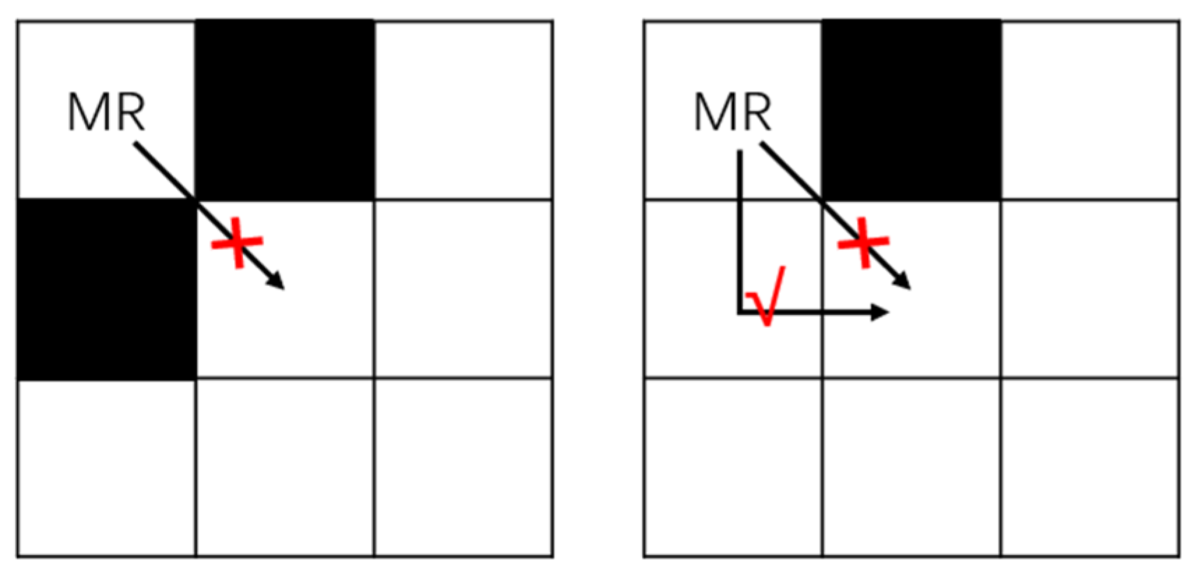
To improve the mobility and path smoothness of the mobile robot, an eight-neighborhood locomotion mode is adopted, allowing the robot to move from the current grid cell to any of its eight adjacent cells. To prevent the path from crossing obstacle corners and generating infeasible or unsafe trajectories, a “no corner-cutting” constraint is introduced, as shown in Figure 11.

5.1.3. Path Processing

In the discrete paths generated by the algorithm, some nodes have little influence on the overall path and can be considered redundant. These redundant nodes not only increase the path length but also reduce the smoothness and feasibility of the path. Therefore, redundant nodes need to be removed appropriately.

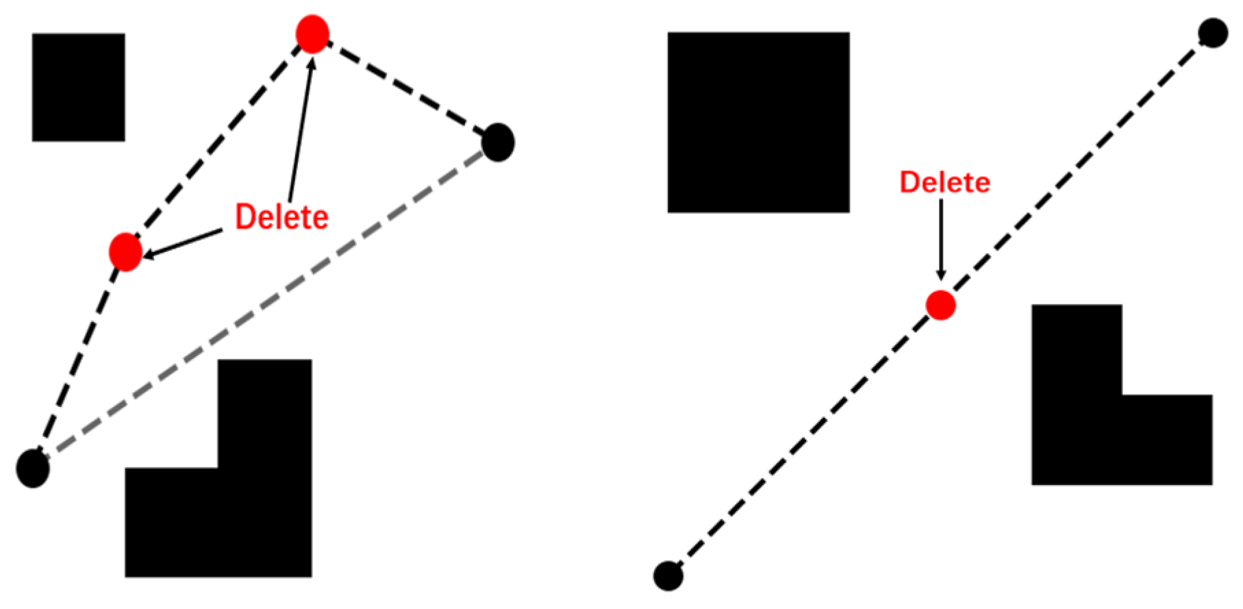
Two deletion strategies are adopted in this study, as shown in Figure 12:

(1)

If there are no obstacles around a local turning point and the new path formed by directly connecting its neighboring nodes still satisfies safety and feasibility requirements, the turning point can be removed.

(2)

If adjacent path nodes are collinear, only the start and end points of the line segment are retained while the intermediate nodes are removed, reducing the number of nodes without changing the geometric shape of the path.

5.1.4. Obstacle Inflation Processing

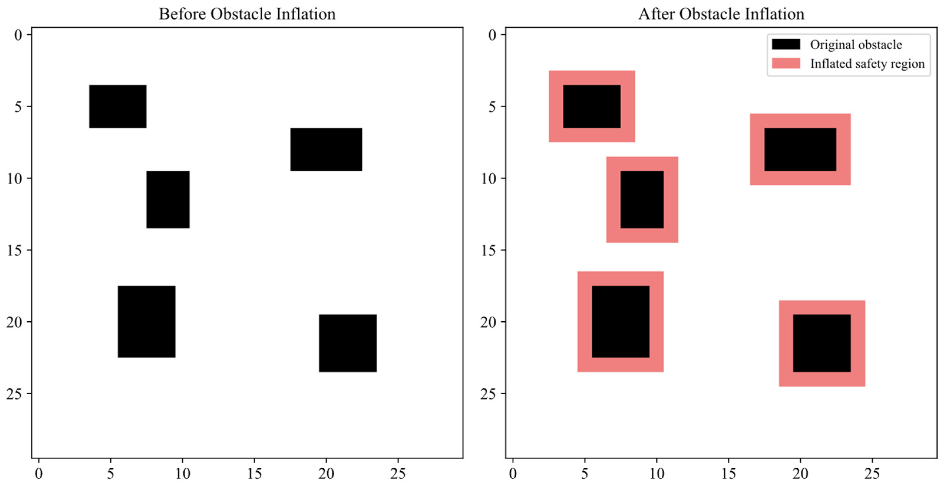
In grid map path planning, if the mobile robot is directly treated as a point mass during search, the generated path only satisfies ideal geometric obstacle avoidance and does not fully consider the robot’s body size and safe clearance. For the three-wheel omnidirectional mobile robot, although it can move laterally and rotate in place and is less constrained by the turning radius, the effect of the robot’s body size on path traversability still needs to be considered when it moves near obstacles or passes through narrow regions. Therefore, before path planning, obstacle inflation is applied to the original grid map in this study. The robot body size and safety margin are equivalently added to the obstacle regions, so that the obstacle boundaries expand outward by a certain distance. After inflation, the algorithm searches for a path on the new grid map. This keeps a safe distance between the planned path and the obstacles and improves the practical executability and safety of the path without clearly increasing algorithm complexity.

Figure 13 shows the obstacle inflation map. As shown in the figure, after inflation, the occupied area of the original obstacles expands outward, and narrow passages as well as regions close to obstacle boundaries are further restricted. When the path planning algorithm searches on the inflated map, it can avoid generating paths that are too close to the obstacle boundaries, which improves path safety and engineering feasibility.

5.2. Path Planning Experimental Results and Analysis

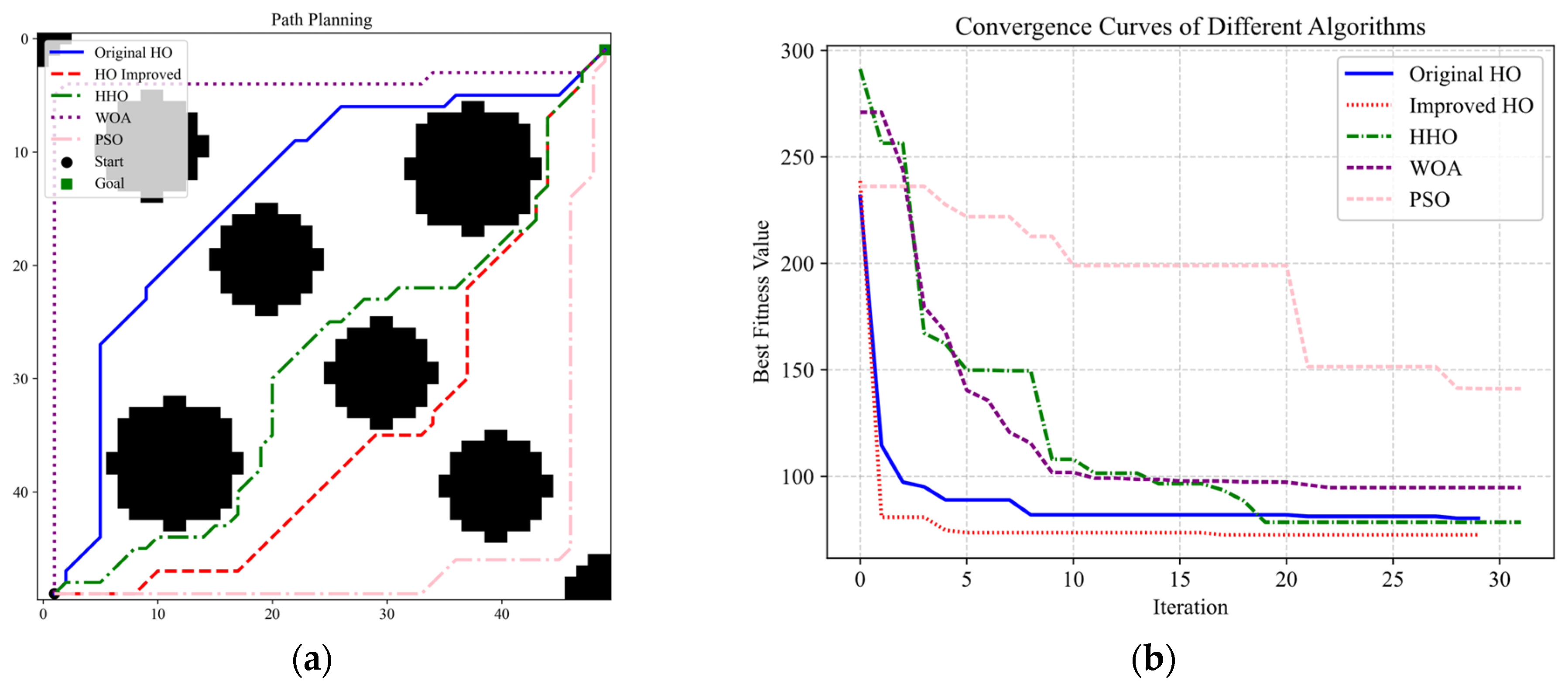
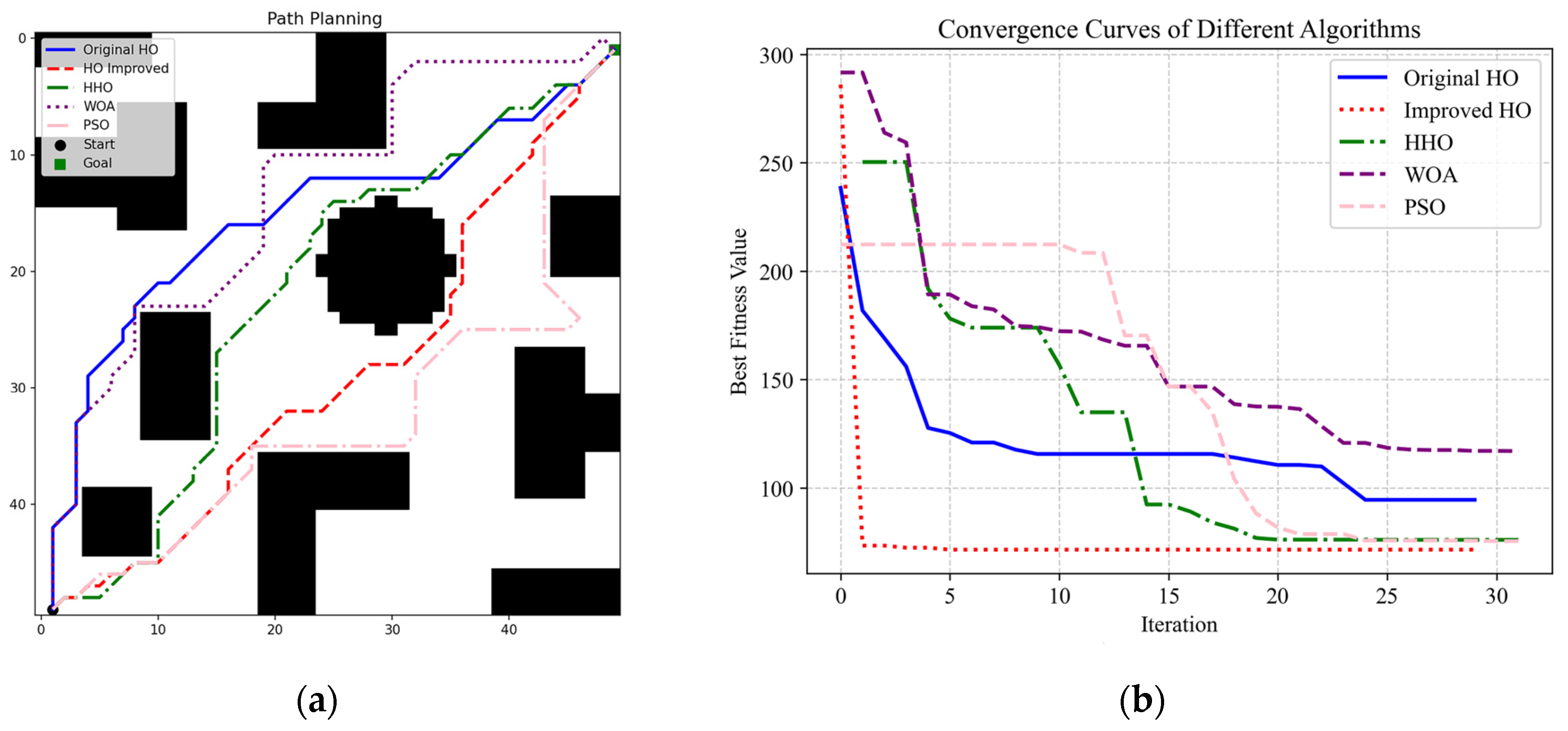
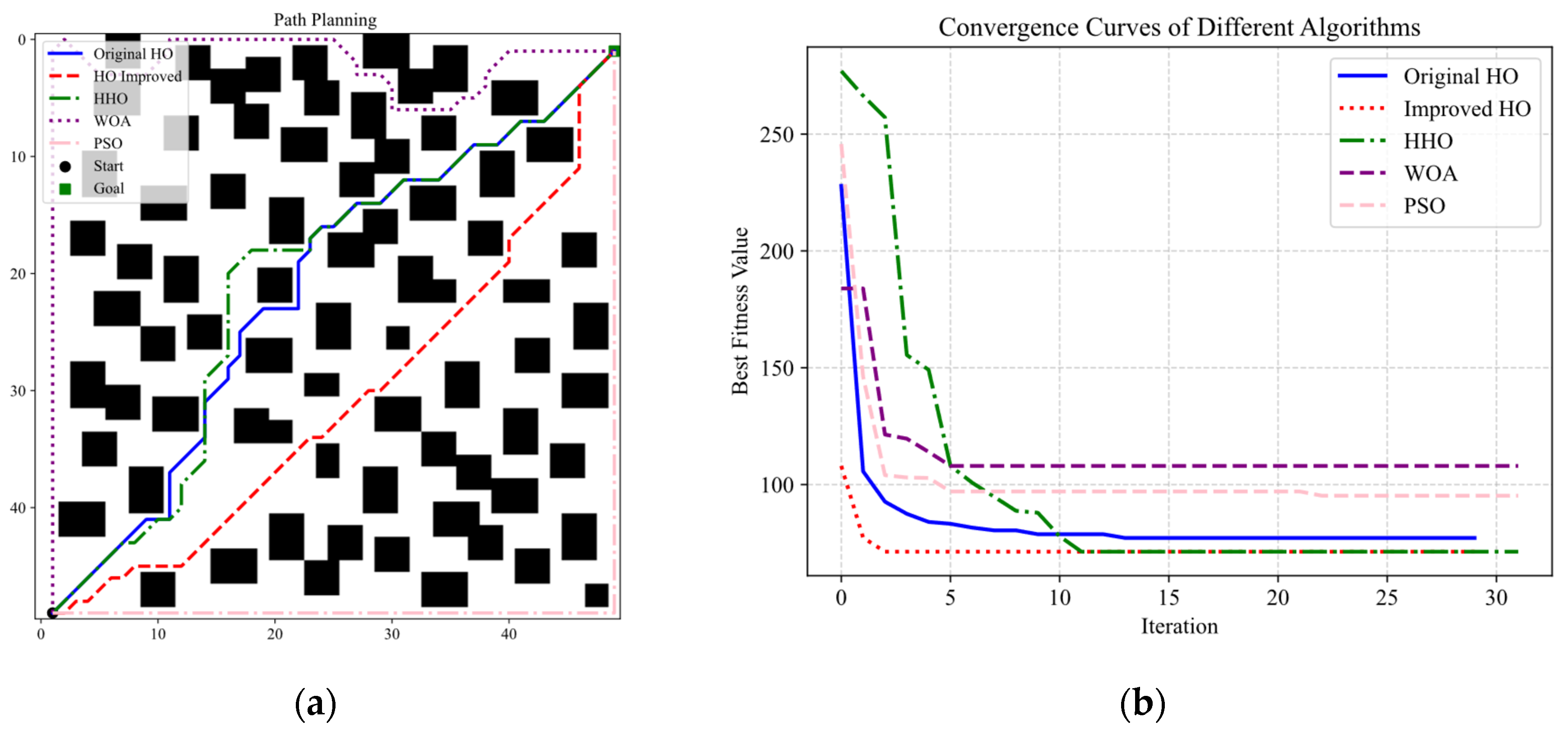
To verify the performance of the improved algorithm in path planning, three grid maps with different obstacle distributions were constructed for testing. IHO was compared with HO, HHO, WOA, and PSO to evaluate the optimization ability and path planning quality of different algorithms in complex environments. The population size was set to 20, and the maximum number of iterations was set to 30. Figure 14, Figure 15 and Figure 16 show the optimal paths and convergence curves of different algorithms in the three environments.

Grid map (I): Symmetric obstacle distribution;

Grid map (II): Asymmetric obstacle distribution;

Grid map (III): Dense obstacle distribution.

As shown in Figure 14a, Figure 15a and Figure 16a, all algorithms can find a path from the start point to the goal point in the three obstacle environments, but the path quality differs clearly. HHO obtains relatively short paths, but its paths contain more turning points and show limited smoothness. WOA and PSO produce clear detours or winding paths in some environments, which increases the path length. In contrast, the paths planned by IHO are more compact. IHO avoids obstacles effectively and reduces unnecessary detours, so its paths are closer to the global optimum. In the dense obstacle environment shown in Figure 16a, IHO still maintains good obstacle avoidance ability and path continuity, which shows its strong path search ability under complex obstacle distributions.

Figure 14b, Figure 15b and Figure 16b show that the fitness value of IHO decreases rapidly in the early iterations and becomes stable within fewer iterations, indicating faster convergence speed. In contrast, some comparative algorithms converge more slowly and still show fluctuations or stagnation in the middle and later iterations. This indicates that they are more easily affected by local optima or unstable search directions. These results show that the improved hippopotamus optimization algorithm (IHO) has stronger global exploration ability and convergence stability, and can effectively avoid local optima to obtain more reasonable planned paths.

To reduce randomness, each algorithm was independently run 10 times on the three maps. The path lengths were recorded, and the best value, worst value, mean, and standard deviation were calculated.

Table 6. Simulation results of Environment I.

	Best	Worst	Mean	Std
HO	79.0122	92.4853	89.9469	4.9321
IHO	78.4264	81.9411	79.2075	1.2952
HHO	78.4264	81.9411	80.1838	1.7574
WOA	94.2426	96.4853	95.3255	0.7593
PSO	81.0122	117.3969	92.2340	13.0566

,

Table 7. Simulation results of Environment II.

	Best	Worst	Mean	Std
HO	79.0122	100.7696	86.2646	10.2565
IHO	73.1543	73.1543	73.1543	0.0000
HHO	73.1543	77.8406	74.7164	2.2091
WOA	91.4975	112.4264	102.5073	8.5789
PSO	75.1543	97.0538	83.1208	9.8859

and

Table 8. Simulation results of Environment III.

	Best	Worst	Mean	Std
HO	73.1543	77.8406	75.3022	2.1567
IHO	73.1543	73.1543	73.1543	0.0000
HHO	73.1543	73.1543	73.1543	0.0000
WOA	76.6690	106.3848	101.1965	10.9811
PSO	96.0000	96.0000	96.0000	0.0000

show the comparison results of the optimal path lengths in the three maps.

Based on Table 6, Table 7 and Table 8, IHO obtains shorter average path lengths in all three experimental environments. In Environment I, the average path length of IHO is 79.2075, which is about 11.9%, 1.2%, 16.9%, and 14.1% shorter than those of HO, HHO, WOA, and PSO, respectively. In Environment II, the average path length of IHO is 73.1543, which is about 15.2%, 2.1%, 28.6%, and 12.0% shorter than those of HO, HHO, WOA, and PSO, respectively. In Environment III, the average path length of IHO is 73.1543, which is the same as that of HHO, and is about 2.9%, 27.7%, and 23.8% shorter than those of HO, WOA, and PSO, respectively. These results show that IHO can obtain high-quality paths under different obstacle distributions. In more complex environments such as Environment II and Environment III, IHO shows a clearer advantage in path length over WOA and PSO.

In terms of standard deviation, IHO maintains a low standard deviation in the three environments, indicating good stability and robustness over multiple independent runs. In Environment II and Environment III, the standard deviation of IHO is 0, which indicates that the algorithm can stably converge to the same final path length in these two environments. This further shows the strong convergence stability of the proposed algorithm.

The results show that the proposed IHO algorithm can obtain high-quality paths under different obstacle distributions and achieves good comprehensive performance in both path length and stability. In particular, in more complex environments such as Environment II and Environment III, IHO shows a clearer path length advantage over WOA and PSO, demonstrating stronger global exploration ability and path optimization ability.

Table 9. Simulation results of algorithm performance in Environment I.

	Path Turning Points	Average Runtime/s	Average Iteration to Best
HO	8.66	11.8437	12.5
IHO	16.5	23.3653	10.83
HHO	18	6.0687	22.50
WOA	4.33	9.4505	24.00
PSO	13.83	11.2271	27.50

,

Table 10. Simulation results of algorithm performance in Environment II.

	Path Turning Points	Average Runtime/s	Average Iteration to Best
HO	15.00	19.7528	22.67
IHO	14.00	14.4808	4.00
HHO	15.67	3.4669	23.67
WOA	19.00	8.7033	26.67
PSO	19.67	11.2691	15.33

and

Table 11. Simulation results of algorithm performance in Environment III.

	Path Turning Points	Average Runtime/s	Average Iteration to Best
HO	21.67	6.1854	10.67
IHO	15.00	8.1581	2.33
HHO	15.00	1.3175	12.33
WOA	22.00	1.9935	12.67
PSO	1.00	0.4768	8.33

present the average algorithm performance and path quality over ten independent runs. IHO keeps a relatively low average number of path turning points in all three environments, which indicates good path continuity. Some algorithms produce fewer turning points in certain environments. However, the path length results show that this usually comes with detours or longer paths. In contrast, IHO maintains a reasonable number of turning points while obtaining shorter paths.

In terms of average runtime, IHO shows different behavior across the three environments. In Environment I and Environment III, the runtime of IHO is higher than that of the comparative algorithms because the nonlinear adaptive weight factor and the lens opposition-based learning strategy introduce extra computation. In Environment II, the runtime of IHO is lower than that of the original HO. The actual runtime in path planning depends not only on the algorithm update process, but also on candidate path quality, the number of obstacle detection operations, and repeated path evaluations. This shows that the stronger search ability of IHO can reduce invalid path evaluations and repeated searches to some extent, which partly offsets the computational cost introduced by the improvement strategies.

For the average iteration to best, IHO reaches the optimal result quickly in all three environments, especially in Environment II and Environment III. Overall, IHO shows good comprehensive performance in path length, path turning points, convergence speed, and stability. This verifies the effectiveness of the proposed improvement strategies in complex path planning tasks.

The experimental results show that IHO has clear overall advantages in path length, convergence speed, and result stability, which confirms its effectiveness, stability, and application feasibility in global path planning.

6. Conclusions

This paper proposes an improved hippopotamus optimization (IHO) algorithm to address the low search accuracy and insufficient stability of mobile robot path planning in complex environments. In IHO, Tent chaotic mapping is introduced to enhance population diversity and strengthen global exploration; a nonlinear adaptive weight factor balances global exploration and local exploitation; and a lens opposition-based learning strategy prevents the algorithm from getting trapped in local optima, improving its robustness. Experimental results show that compared with the HO algorithm, IHO achieves significantly higher solution accuracy and stability and outperforms other comparative algorithms such as HHO in overall optimization performance. In the robot path planning simulation experiments, IHO shows better performance in path length, convergence speed, and result stability. It also maintains a reasonable number of path turning points while obtaining shorter paths, and generates shorter and more stable paths with better practical executability.

The proposed IHO algorithm still has some limitations. On one hand, the introduction of multiple improvement strategies increases computational complexity to some extent. On the other hand, this study focuses mainly on static environment path planning, and its adaptability to dynamic obstacles remains to be further improved.

Future research will address these issues by further optimizing the algorithm’s computational efficiency and integrating dynamic environmental perception and real-time obstacle updating mechanisms, expanding its application to dynamic scenarios and multi-robot cooperative path planning in complex real-world environments.

References

1. Tao, Y.; Gao, H.; Ren, F.; Chen, C.; Wang, T.; Xiong, H.; Jiang, S. A mobile service robot global path planning method based on ant colony optimization and fuzzy control. Appl. Sci. 2021, 11, 3605. [Google Scholar] [CrossRef]
2. Liu, L.; Wang, X.; Yang, X.; Liu, H.; Li, J.; Wang, P. Path planning techniques for mobile robots: Review and prospect. Expert. Syst. Appl. 2023, 227, 120254. [Google Scholar] [CrossRef]
3. Qin, H.; Shao, S.; Wang, T.; Yu, X.; Jiang, Y.; Cao, Z. Review of autonomous path planning algorithms for mobile robots. Drones 2023, 7, 211. [Google Scholar] [CrossRef]
4. Jiang, H.; Fang, W.; Xu, T.; Xu, H.; Chen, L.; Zhou, L.; Deng, Q. Optimal indoor evacuation path-planning model based on Dijkstra’s algorithm. J. Tsinghua Univ. (Sci. Technol.) 2025, 65, 742–749. [Google Scholar] [CrossRef]
5. Zhang, B.; Cai, X.; Li, G.; Li, X.; Peng, M.; Yang, M. A modified A* algorithm for path planning in the radioactive environment of nuclear facilities. Ann. Nucl. Energy 2025, 214, 111233. [Google Scholar] [CrossRef]
6. Huang, A.; Zhou, M.; Liu, M.; Pan, Y.; Guo, J.; Hu, Y. Adaptive Path Planning for Robotic Winter Jujube Harvesting Using an Improved RRT-Connect Algorithm. Agriculture 2025, 16, 47. [Google Scholar] [CrossRef]
7. Li, X.; Tong, Y. Path planning of a mobile robot based on the improved RRT algorithm. Appl. Sci. 2023, 14, 25. [Google Scholar] [CrossRef]
8. Li, C.; Zhang, Y.; Song, D.; Zhang, N.; Chen, L.; Yang, J.; Wang, L.; Zhai, X.B. UGV Formation Path Planning Based on DRL-DWA in Off-Road Environments. Appl. Sci. 2025, 15, 12212. [Google Scholar] [CrossRef]
9. Teng, Y.; Feng, T.; Li, J.; Chen, S.; Tang, X. A dual-layer symmetric multi-robot path planning system based on an improved neural network-DWA algorithm. Symmetry 2025, 17, 85. [Google Scholar] [CrossRef]
10. Liu, C.; Wu, L.; Xiao, W.; Li, G.; Xu, D.; Guo, J.; Li, W. An improved heuristic mechanism ant colony optimization algorithm for solving path planning. Knowl.-Based Syst. 2023, 271, 110540. [Google Scholar] [CrossRef]
11. Rosas-Carrillo, A.S.; Solís-Santomé, A.; Silva-Sánchez, C.; Camacho-Nieto, O. UAV path planning using an adaptive strategy for the particle swarm optimization algorithm. Drones 2025, 9, 170. [Google Scholar] [CrossRef]
12. Guo, Z.; Zhang, T.; Su, H.; Jie, S.; Tu, Y.; Li, Y. Research on Mobile Robot Path Planning Using Improved Whale Optimization Algorithm Integrated with Bird Navigation Mechanism. World Electr. Veh. J. 2025, 16, 676. [Google Scholar] [CrossRef]
13. Feng, W.-Q.; Yang, Y.; Yang, L.-F.; Fu, Y.-J.; Xu, K.-J. Unmanned Aerial Vehicle Logistics Distribution Path Planning Based on Improved Grey Wolf Optimization Algorithm. Symmetry 2025, 17, 2178. [Google Scholar] [CrossRef]
14. Cai, C.; Jia, C.; Nie, Y.; Zhang, J.; Li, L. A path planning method using modified harris hawks optimization algorithm for mobile robots. PeerJ Comput. Sci. 2023, 9, e1473. [Google Scholar] [CrossRef]
15. Cao, M.; Zhao, W.; Chen, Z. Robot path planning by fusing particle swarm algorithm and improved grey wolf algorithm. J. Syst. Simul. 2023, 35, 1768–1775. [Google Scholar] [CrossRef]
16. He, J.; He, Z.; Liu, J.; Zhang, Y.; Zhang, F.; Liang, F.; Wang, T.; Xiao, L.; Wang, X. An effective power optimization approach based on whale optimization algorithm with two-populations and mutation strategies. Chin. J. Electron. 2024, 33, 423–435. [Google Scholar] [CrossRef]
17. Xue, J.; Shen, B. Dung beetle optimizer: A new meta-heuristic algorithm for global optimization: J. Xue, B. Shen. J. Supercomput. 2023, 79, 7305–7336. [Google Scholar] [CrossRef]
18. Amiri, M.H.; Mehrabi Hashjin, N.; Montazeri, M.; Mirjalili, S.; Khodadadi, N. Hippopotamus optimization algorithm: A novel nature-inspired optimization algorithm. Sci. Rep. 2024, 14, 5032. [Google Scholar] [CrossRef]
19. Wang, H.; Binti Mansor, N.N.; Mokhlis, H.B. Novel hybrid optimization technique for solar photovoltaic output prediction using improved hippopotamus algorithm. Appl. Sci. 2024, 14, 7803. [Google Scholar] [CrossRef]
20. Maurya, P.; Tiwari, P.; Pratap, A. Application of the hippopotamus optimization algorithm for distribution network reconfiguration with distributed generation considering different load models for enhancement of power system performance. Electr. Eng. 2025, 107, 3909–3946. [Google Scholar] [CrossRef]
21. Baihan, A.; Alutaibi, A.I.; Alshehri, M.; Sharma, S.K. Sign language recognition using modified deep learning network and hybrid optimization: A hybrid optimizer (HO) based optimized CNNSa-LSTM approach. Sci. Rep. 2024, 14, 26111. [Google Scholar] [CrossRef]
22. Pan, J.; Ke, N.; Shen, N. Unmanned Aerial Vehicles 3D Path Planning Based on Improved Hippopotamus Optimization. In Proceedings of the 2025 8th International Conference on Advanced Algorithms and Control Engineering (ICAACE), Shanghai, China, 21–23 March 2025; pp. 403–418. [Google Scholar]
23. Han, Y.; Wang, H. Multi-USV Cooperative Path Planning via FSM-based Distance Field and Enhanced Hippopotamus Optimization. Int. J. Nav. Arch. Ocean. 2025, 18, 100714. [Google Scholar] [CrossRef]
24. Yanchun, G.; Haiyan, L.; Lei, X.; Wanqiang, S. Adaptive Dynamic Learning Chicken Swarm Optimization Algorithm. J. Comput. Eng. Appl. 2020, 56, 36–45. [Google Scholar] [CrossRef]
25. Yang, Y.; Ling, M. Parameter identification of proton exchange membrane fuel cell model based on improved chicken swarm optimization algorithm. Acta Energiae Solaris Sin. 2023, 44, 269–278. [Google Scholar] [CrossRef]
26. Zhao, J.; Zhu, X.; Meng, X.; Wu, X. Application of Improved Whale Optimization Algorithm in Time-optimal Trajectory Planning of Manipulator. Mech. Sci. Technol. Aerosp. Eng. 2023, 42, 388–395. [Google Scholar] [CrossRef]
27. Chauhan, S.; Vashishtha, G.; Kumar, A. A symbiosis of arithmetic optimizer with slime mould algorithm for improving global optimization and conventional design problem. J. Supercomput. 2022, 78, 6234–6274. [Google Scholar] [CrossRef]
28. Hu, J.; Zheng, Y.; Wang, S.; Zhou, C. Improved Particle Swarm Optimization Based on Fuzzy Controller Fusion of Multiple Strategies for Multi-Robot Path Planning. Big Data Cogn. Comput. 2025, 9, 229. [Google Scholar] [CrossRef]
29. Xin, G.; Shi, L.; Long, G.; Pan, W.; Li, Y.; Xu, J. Mobile robot path planning with reformative bat algorithm. PLoS ONE 2022, 17, e0276577. [Google Scholar] [CrossRef]
30. Shao, Y.; Zhu, L.; Su, C.; Wang, J. An improved whale optimization algorithm for multi-robot path planning. Eng. Optim. 2025, 57, 1615–1641. [Google Scholar] [CrossRef]
31. Agrawal, S.; Patle, B.K.; Sanap, S. A novel technique for drone path planning based on a neighborhood dragonfly algorithm. Sensors 2025, 25, 863. [Google Scholar] [CrossRef] [PubMed]
32. Liu, H.; Luo, J.; Zhang, L.; Yu, H.; Liu, X.; Wang, S. Research on traversal path planning and collaborative scheduling for corn harvesting and transportation in hilly areas based on dijkstra’s algorithm and improved harris hawk optimization. Agriculture 2025, 15, 233. [Google Scholar] [CrossRef]
33. Danfeng, S.; Xufeng, L.; Gang, Z.; Zumao, H. Automated guided vehicle path planning by dynamically adjusting ant colony algorithm heuristic factor. J. Xi’an Polytech. Univ. 2023, 37, 93–102. [Google Scholar] [CrossRef]
Figure 1. Mechanical structure diagram of the three-wheel omnidirectional robot; (a) front view of the robot; (b) top view of the robot.
Robotics 15 00104 g001
Figure 2. Omnidirectional mobile robot coordinate system and simulation diagram; (a) robot coordinate system; (b) robot simulation model: red-X, green-Y, blue-Z.
Robotics 15 00104 g002
Figure 3. Path planning diagram of mobile robot.
Robotics 15 00104 g003
Figure 4. Probability density distribution comparison of three chaotic maps.
Robotics 15 00104 g004
Figure 5. Convergence curves for Tent chaotic map.
Robotics 15 00104 g005
Figure 6. Exponential adaptive weight curves under different k.
Robotics 15 00104 g006
Figure 7. Convergence curves for adaptive weight factor.
Robotics 15 00104 g007
Figure 8. Convergence curves for LOBL.
Robotics 15 00104 g008
Figure 9. The convergence curves for test functions.
Robotics 15 00104 g009
Figure 10. A 10 × 10 two-dimensional grid map. (a) Two-dimensional array; (b) grid map.
Robotics 15 00104 g010
Figure 11. Prohibition of corner constraint.
Robotics 15 00104 g011
Figure 12. Deletion strategy.
Robotics 15 00104 g012
Figure 13. Inflated obstacle map.
Robotics 15 00104 g013
Figure 14. The 50 × 50 grid map (I); (a) optimal paths of different algorithms; (b) convergence curves of different algorithms.
Robotics 15 00104 g014
Figure 15. The 50 × 50 grid map (II); (a) optimal paths of different algorithms; (b) convergence curves of different algorithms.
Robotics 15 00104 g015
Figure 16. The 50 × 50 grid map (III); (a) optimal paths of different algorithms; (b) convergence curves of different algorithms.
Robotics 15 00104 g016