Article

Parameter-Adaptive Event-Triggered Sliding Mode Control for a Mobile Robot

1
National Key Laboratory of Digital Control and System Engineering (DCSELab), Ho Chi Minh City University of Technology (HCMUT), 268 Ly Thuong Kiet Street, District 10, Ho Chi Minh City 700000, Vietnam
2
Faculty of Center for Continuing Education, Ho Chi Minh City University of Transport, Ho Chi Minh City 700000, Vietnam
3
Faculty of Mechanical Engineering, Ho Chi Minh City University of Technology (HCMUT), 268 Ly Thuong Kiet, District 10, Ho Chi Minh City 700000, Vietnam
4
Vietnam National University Ho Chi Minh City, Linh Trung Ward, Thu Duc District, Ho Chi Minh City 700000, Vietnam
5
Faculty of Electronics and Telecommunication, Saigon University, Ho Chi Minh City 700000, Vietnam
*
Author to whom correspondence should be addressed.
Robotics 2022, 11(4), 78; https://doi.org/10.3390/robotics11040078
Submission received: 4 May 2022 / Revised: 11 July 2022 / Accepted: 28 July 2022 / Published: 2 August 2022
(This article belongs to the Section Sensors and Control in Robotics)

Abstract

:
Mobile robots have played a vital role in the transportation industries, service robotics, and autonomous vehicles over the past decades. The development of robust tracking controllers has made mobile robots a powerful tool that can replace humans in industrial work. However, most of the traditional controller updates are time-based and triggered at every predetermined time interval, which requires high communication bandwidth. Therefore, an event-triggered control scheme is essential to release the redundant data transmission. This paper presents a novel parameter-adaptive event-trigger sliding mode to control a two-wheeled mobile robot. The adaptive control scheme ensures that the mobile robot system can be controlled accurately without the knowledge of physical parameters. Meanwhile, the event trigger sliding approach guarantees the system robustness and reduces resource usage. A simulation in MATLAB and an experiment are carried out to validate the efficiency of the proposed controller.

1. Introduction

In recent years, the rapid development of autonomous systems has given rise to the application of mobile robots in many field applications. The massive surge in the implementation of mobile robots is thanks to mobility, reliability, and the fact that they can operate without any assistance from human operators. The term “mobile robots” is not exclusively limited to any particular locomotion designs; there are numerous types of mobile robots on the ground, underwater, or in the air [1,2,3,4,5]. However, one of the most extensively researched mobile robots is the two-wheeled differential drive robot, which is in demand for many tasks such as transportation in factory storage, restaurants, and hospitals; and in servicing and guiding people in museums and airports [6,7,8,9].
In order for mobile robots to operate automatically and reliably, it is necessary to derive a robust controller for trajectory tracking. There have been many works on the tracking control for two-wheeled mobile robots throughout the years, in both kinematic and dynamic aspects [10,11,12,13,14,15]. In order to address the problem of external disturbances, an adaptive-based controller for the dynamic model has been proposed in some literature [16,17,18]. Imitation learning is also a viable solution to overcome the instability caused by the disturbances [19,20,21]. To further improve the control performance, Fukao et al. [22] implemented an adaptive tracking controller for both the kinematic and dynamic modeling to estimate the presence of unknown parameters. Despite the excellent performance, these aforementioned controllers utilized the traditional sampling technique in which the sampling time is kept constant. It is widely used in many practical applications due to its simplicity. However, the time-event control is bandwidth-consuming for data transmission since it requires computations at every periodic instant regardless of the redundant data, leading to a waste of resources [23,24,25]. This control scheme is also considerably detrimental in a network control system that induces time delays in data transmission and packet data dropout. A TCP/IP model with four layers can solve the negative effect of the packet data dropout; however, it worsens the time delays, thus degrading the control performance. Therefore, the event-triggered control scheme has been introduced in much research to overcome these drawbacks [26,27,28,29].
There are many types of controllers that can be paired up with the event-triggered scheme to tackle the other issues. When combined with the traditional PID, it has been proved to be very effective in reducing the consumption of CPU resources [30,31,32]. In [33,34,35], an event-triggered scheme is utilized to achieve the convergence of the Lyapunov function in improving the robustness of the controller. The alternative is sliding mode control (SMC); SMC is a control technique famous for its robustness [36,37,38]. Despite the fact that the mobile robot can be controlled by many different schemes such as neural network [39,40,41,42], linear quadratic regulator (LQR) [43,44], or the quadratic curve (QC) algorithm in our previous study [45], SMC still remains a popular approach for its matched disturbances rejection [46,47,48], and nullifying of uncertainty properties [49]. Consequently, SMC has been used widely in many non-linear systems nowadays.
In our previous study, a commercial mobile robot called Pioneer DX3 was controlled by the QC path tracking algorithm. Despite the high tracking accuracy, the tracking controller did not consider the uncertainty in some parameters of the mobile robot. For instance, continuous usage would cause the wheel tires to wear down, thus reducing the radius of the wheels, which affects the accuracy of the control parameters. In some cases, physical parameters which cannot be measured accurately due to the lack of specialized equipment, degrading the control performance of the model-based controller. Thus, it is essential to implement an adaptive scheme to overcome the negative effect of the unknown parameters. Regarding the control scheme, the mobile robot is expected to be teleoperated, where a computer plays the role of the high-level controller, implementing the tracking algorithm and communicating via wireless connection with a microcontroller, acting as a low-level controller. The capability to reduce the computation load of the event-triggered control strategy is extremely valuable to the teleoperation process in terms of neglecting the adverse effect of induced time delays. Motivated by the advantages of the event-triggered scheme and the SMC, in this paper, a parameter adaptive event-triggered sliding mode control is proposed for tracking control of the mobile robot in the presence of uncertainties. Even though a computer implementing the proposed controller communicates with a microcontroller board through a wired connection which does not induce time delays in data transmission, the communication rate and the computation bandwidth of the microcontroller are limited. Thus, it requires the computation reduction of the proposed controller.
The paper is organized as follows. Section 2.1 proposes a well-known kinematic model for a mobile robot from our previous study; then a parameter-adaptive sliding mode controller is constructed base on the kinematic model to control the mobile robot. Section 2.2 describes the combination of the parameter-adaptive sliding mode control approach with the event-trigger control method to control the mobile robot. Section 3 gives a description of the simulation and experiment in various scenarios. Finally, Section 4 gives the results and a detailed analysis of the proposed controller.
The main contributions of this paper are as follows:
(1)
A novel event-triggered sliding mode controller for the kinematic model of a mobile robot is designed to reduce the computational work of the microcontroller.
(2)
An adaptive scheme is combined with the event-triggered sliding mode controller to estimate the parameters of the mobile robot. This ensures that the control performance of the proposed control is kept robust in the presence of uncertainties and unknown parameters.
(3)
Simulation and experiment results in different scenarios are given to validate the proposed controller.

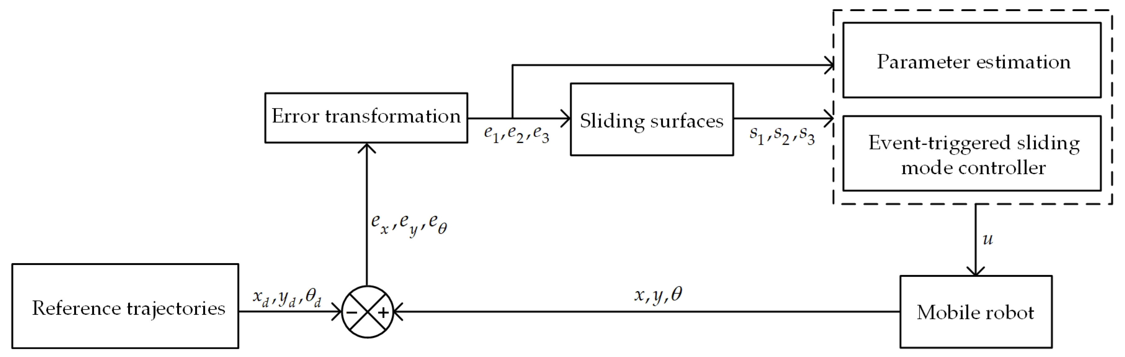
2. Controller Design

2.1. Parameter-Adaptive Sliding Mode Controller

Consider a well-known kinematic model for a mobile robot, as shown in Figure 1a [45]. The mobile robot is required to track the trajectory generated by a virtual robot, as shown in Figure 1b.
x ˙ c y ˙ c θ ˙ c = r 2 cos θ c r 2 cos θ c r 2 sin θ c r 2 sin θ c r W r W ω r ω l
where ω r and ω l are the angular velocities of the right and left wheel; r is the wheel radius; W is the distance between two wheels; x c , y c , and θ c are the positions of the mobile robot.
The relationship between v , ω and ω r , ω l is expressed in the following form:
ω r ω l = 1 r W 2 r 1 r W 2 r v ω
where v and ω are the linear and angular velocities of the mobile robot, respectively.
By defining the tracking errors between the current pose and the reference trajectories as e x x c x r , e y y c y r , e θ θ c θ r in the global coordinates where x r , y r and θ r are the positions of the reference mobile robot, the tracking errors with respect to the robot coordinate are given as follows:
e 1 e 2 e 3 = cos θ c sin θ c 0 sin θ c cos θ c 0 0 0 1 e x e y e θ
where e 1 ,   e 2 ,   e 3 are the tracking errors between the robot pose and the reference trajectories in the robot coordinate.
The dynamic of the tracking errors is given as follows:
e ˙ 1 e ˙ 2 e ˙ 3 = v 1 0 0 + ω e 2 e 1 1 + v r cos e 3 v r sin e 3 ω r
where v r and ω r are, respectively, the reference linear and angular velocities.
Equation (4) can be rewritten in an affine form as follows:
e ˙ = f e + g e u v
where
e e 1 e 2 e 3 ,   f e v r cos e 3 v r sin e 3 ω r , g e 1 e 2 0 e 1 0 1 , u v v ω
Equation (2) shows that the parameters of r and W are required to be known accurately for achieving the control input u = ω r ω l T   of the mobile robot. However, these parameters are difficult to measure accurately in practice. In reality, continuous usage of the mobile robot can lead to the wearing of the wheel-tire; this might cause the wheel radius to change. Alternatively, the measurement may not be accurate due to the lack of a precision measurement instrument. Therefore, an adaptive-based controller is required to estimate r and W .
By defining a 1 r , b W 2 r and using Equation (2), the control input u can be calculated based on the estimation of a and b   as follows:
u = ω r ω l = a ^ b ^ a ^ b ^ v ω = a + a ˜ b + b ˜ a + a ˜ b b ˜ v ω
where a ^ and b ^ are, respectively, the estimated parameters of a ,   b ,   and the terms a ˜ a ^ a ,   b ˜ b ^ b .
From Equation (6), the control input u v for Equation (5) can be calculated as follows:
u v = v ω = a + a ˜ b + b ˜ a + a ˜ b b ˜ 1 ω r ω l  
Substituting Equation (6) into Equation (4) and writing it in the affine form, it can be obtained as
e ˙ = f e + g e + g ˜ e u v
where
g ˜ e a ˜ a b ˜ b e 2 0 b ˜ b e 1 0 b ˜ b
In order to guarantee the convergence of all the tracking errors e = e 1 e 2 e 3 T , let us define the sliding surface for the system of Equation (8) as follows:
s = s 1 s 2 s 3 T e 1 + e 2 e 1 e 2 e 1 e 2 + e 3
Taking the first time derivative of the sliding surface, it yields:
s ˙ = f ¯ e + g ¯ e + g e u v
where
g ¯ e 1 e 2 e 1 1 e 2 + e 1 1 e 2 + e 1 1 ,   f ¯ e v r cos e 3 + v r sin e 3 v r cos e 3 sin e 3 ω r + v r cos e 3 sin e 3 , g e a ˜ a b ˜ b e 2 e 1 a ˜ a b ˜ b e 2 + e 1 a ˜ a b ˜ b e 2 + e 1 1  
Assumption 1.
Assume that there exists a positive constant μ so that it satisfies b μ > 0 .
Theorem 1.
Consider the system in Equation(8). Supposing that Assumption 1 is satisfied, the following control input and parameter adaptation law will lead to the convergence of the sliding surfaces s  to zero while the parameter estimation’s errors a ˜ and b ˜ remain within the boundaries.
u v = g ¯ e 1 f ¯ e + k s i g n s
a ^ ˙ = γ 1 v s 1 + s 2 + s 3 b ^ ˙ = γ 2 ω s 1 e 2 e 1 + s 2 e 2 + e 1 + s 3 e 2 + e 1 1 + f b b ^
where k ,   γ 1 , γ 2 are positive constants, g ¯ e 1  is the pseudo-inverse of the non-square matrix g ¯ e , and the function f b is defined as follows:
f b b ^ = 0 ,                     b ^ > μ 1 b ^ μ 2 ,       b ^ μ  
Proof of Theorem 1.
Consider a candidate Lyapunov function as follows:
V e , a ˜ , b ˜ = 1 2 s T s + 1 2 γ 1 a a ˜ 2 + 1 2 γ 2 b b ˜ 2
Taking the first-time derivative of the Lyapunov function of Equation (14) and using Equation (10) yields
V ˙ e , a ˜ , b ˜ = s T f ¯ e + g ¯ e + g e u v + 1 γ 1 a a ˜ a ˜ ˙ + 1 γ 2 b b ˜ b ˜ ˙ = s T f ¯ e + g ¯ e u v + s T g e u v + 1 γ 1 a a ˜ a ^ ˙ + 1 γ 2 b b ˜ b ^ ˙ = s T f ¯ e + g ¯ e u v a ˜ a v s 1 + s 2 + s 3 + b ˜ b ω s 1 e 2 e 1 + s 2 e 2 + e 1 + s 3 e 2 + e 1 1 + 1 γ 1 a a ˜ a ^ ˙ + 1 γ 2 b b ˜ b ^ ˙ = s T f ¯ e + g ¯ e u v + a ˜ γ 1 a a ^ ˙ γ 1 v s 1 + s 2 + s 3 + b ˜ γ 2 b b ^ ˙ + γ 2 ω s 1 e 2 e 1 + s 2 e 2 + e 1 + s 3 e 2 + e 1 1
Substituting Equations (11) and (12) into Equation (15) yields:
V ˙ = k s T s i g n s + b ^ b γ 2 b f b b ^
Case 1: If b ^ > μ referring to Equation (13), Equation (16) becomes V ˙ = k s T s i g n s 0 . Taking the second-time derivative of the Lyapunov function, it can be obtained as:
V ¨ = k s ˙ T s i g n s
Case 2: If b ^ μ referring to Equation (13) and Assumption 1, it can be deduced that b ^ b b ^ μ 0 ; therefore one can conclude that V ˙ 0 . The second order derivative of the Lyapunov function is shown as:
V ¨ = k s ˙ T s i g n s + b ^ ˙ b γ 2 b f b b ^ 2 b ^ ˙ b ^ b γ 2 μ b 1 b ^ μ
Consequently, it can be seen that s , a ˜ , b ˜ are bounded in both cases. Equations (17) and (18) also show that V ¨ is bounded. By applying Barbalat’s lemma, it can be proved that e 0 as t . □

2.2. Parameter-Adaptive Event-Triggered Sliding Mode Controller

In this section, an event-triggered controller is proposed to drive the dynamic error of Equation (8) to zero. The event-triggered control strategy only generates the control input if a certain condition is satisfied, leading to a non-constant sampling period.
Consider the control input of Equation (11) expressed in the discrete time as follows:
u v t i = g ¯ e t i 1 f ¯ e t i + k s i g n s t i
where t i is the discrete time instants with i + .
Let us define the event-triggered error in a certain interval t t i ,   t i + 1 as ε t e t e t i . If this error passes a given threshold, the control input value will be updated. Otherwise, it will remain constant during the given interval.
Assumption 2.
Let δ g ¯ e t g ¯ e t i 1 ,   η g e t + g ˜ e t g ¯ e t i 1  and these are bounded such that δ δ ¯ ,   η η ¯   where δ ¯ , η ¯ are positive constants.
Assumption 3.
Assume that f ¯ e t  is a Lipschitz function with respect to its argument such that f ¯ e t δ f ¯ e t i L e t e t i , where L is a positive constant.
Theorem 2.
The tracking errors of the system in Equation(8) converge to zero in finite time if the control input of Equation(19) is updated according to the following triggering rule.
ε < δ k L
Proof of Theorem 2.
Consider the first-time derivative of the sliding surface s ˙ in Equation (10) for the interval t i , t i + 1
s ˙ t = f ¯ e t + g ¯ e t + g e t u v t
For the interval t i , t i + 1 , the control input u v t u v t i . Consequently, the control input of Equation (19) can substitute into Equation (21) to obtain:
s ˙ t = f ¯ e t δ f ¯ e t i δ k s i g n s t i + g e t u v t
To analyze the system stability, the candidate Lyapunov function is taken as in Equation (14)
V e , a ˜ , b ˜ = 1 2 s T s + 1 2 γ 1 a a ˜ 2 + 1 2 γ 2 b b ˜ 2
Taking the first-time derivative of Equation (23) and utilizing Equation (22), it yields:
V ˙ e , a ˜ , b ˜ = s T f ¯ e t δ f ¯ e t i s T δ k s i g n s t i + a ˜ γ 1 a a ^ ˙ γ 1 v s 1 + s 2 + s 3 + b ˜ γ 2 b b ^ ˙ + γ 2 ω s 1 e 2 e 1 + s 2 e 2 + e 1 + s 3 e 2 + e 1 1  
Let us define V ¯ s T f ¯ e t δ f ¯ e t i s T δ k s i g n s t i for further analysis. By applying Assumption 3 and the norm property, V ¯ can be rewritten as:
V ¯ L s e t e t i s δ k = s L ε δ k  
Combining Equations (24) and (25), and utilizing Equation (12), the following expression is obtained:
V ˙ e , a ˜ , b ˜ s L ε δ k + b ^ b γ 2 b f b b ^  
Hence, by using the triggering rule in Equation (20), one can ensure that V ˙ e , a ˜ , b ˜ 0 . This completes the proof of Theorem 2. □
In the design of event-trigger control, there is a possibility that the Zeno phenomenon will occur, which means an infinity of events trigger in a finite-time interval [50]. In order to avoid the Zeno phenomenon, the inter-event time T i = t t i should be proved to have a lower bound [51,52].
Assumption 4.
Assume that the functions f · are locally Lipschitz for some constants such that f e t = L 1 e t , η f e t i = L 2 e t i , η k s i g n s t i = L 3 .
Taking the first-time derivative of the event-triggered error ε t , it yields:
d ε t d t d e t d t d e t i d t f e t + g e t + g ˜ e t u v t i f e t g e t + g ˜ e t g ¯ e t i 1 f ¯ e t i + k s i g n s t i f e t η f e t i η k s i g n s t i
By applying Assumption 4, Equation (27) becomes:
d ε t d t L 1 e t + L 2 e t i + L 3 L 1 ε t + L 1 e t i + L 2 e t i + L 3  
Solving the inequality of Equation (28) for ε t ,   it can give the following expression:
ε t L 1 + L 2 e t i + L 3 e x p L 1 T i 1 L 1  
Substituting the triggering rule in Equation (20) into the left-hand side of Equation (29) and solving for the inter-event time T i , we get the lower bound as follows:
T i 1 L 1 ln δ k L 1 L L 1 + L 2 e t i + L 3 + 1  

3. Simulation and Experimental Description

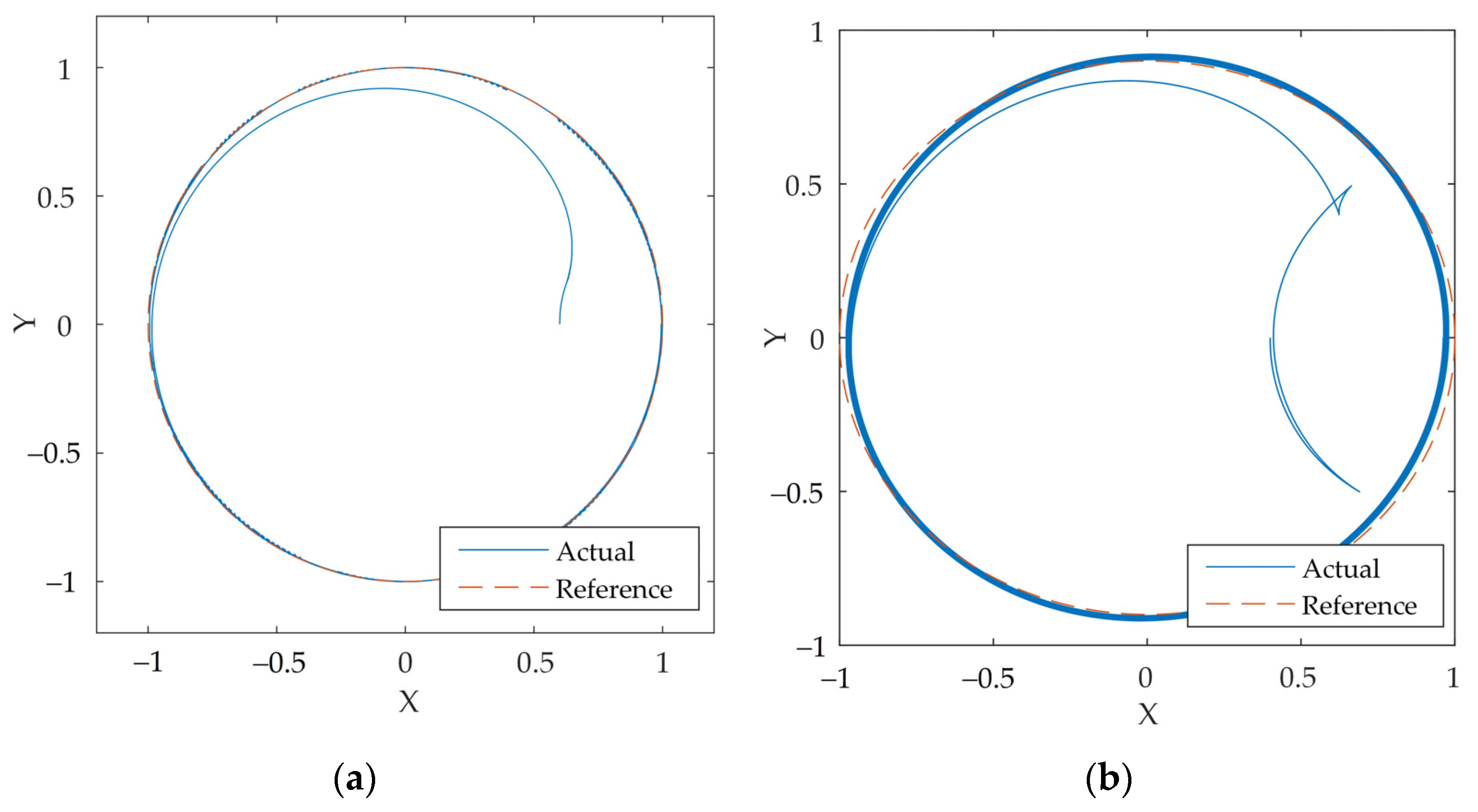
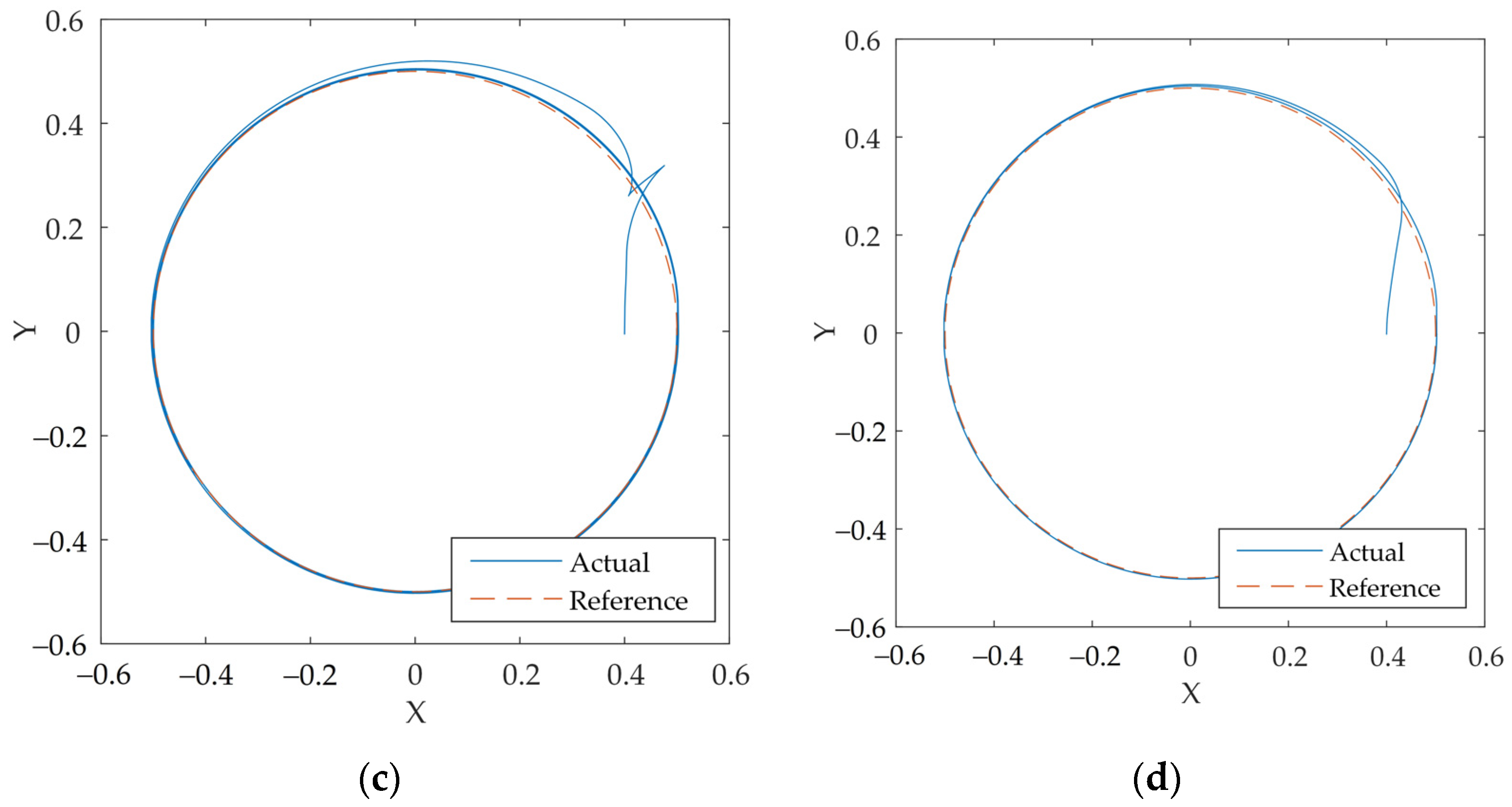
3.1. Simulation Scenario

In this section, simulations are carried out in two different trajectories in MATLAB to evaluate the effectiveness of the proposed controller. The simulation parameters are shown in Table 1. In addition, a block diagram describing the proposed controller implemented on the mobile robot is shown in Figure 2.
The simulations are carried out in two different scenarios to evaluate the performance of the proposed controller. Each scenario follows the same control structure from Figure 2; the only differences are the reference trajectory and the initial values. The bound value for a is chosen as 6 < a < 14 .

3.1.1. Scenario 1

The reference trajectory in this scenario is a circle with a radius of 1 m . The simulation time is 300 s. The initial positions and values for the estimated parameters of the mobile robot are x = 0.6   m and y = 0   m ; a ^ = 8 and b ^ = 1 . The controller gains are selected as k = 0.8 , γ 1 = 5 , γ 2 = 5 .

3.1.2. Scenario 2

In this scenario, the reference trajectory is an ellipse with the value of the major axis a e l l i p s e = 1   m and minor axis b e l l i p s e = 0.9   m . The simulation time is 300 s, which means that the mobile robot moves ten laps of the ellipse, taking 30 s for each lap. The initial positions and values for the estimated parameters of the mobile robot are x = 0.4   m and y = 0   m ; a ^ = 8 and b ^ = 3 . The controller gains are chosen as k = 0.8 ,   γ 1 = 15 ,   γ 2 = 15 .

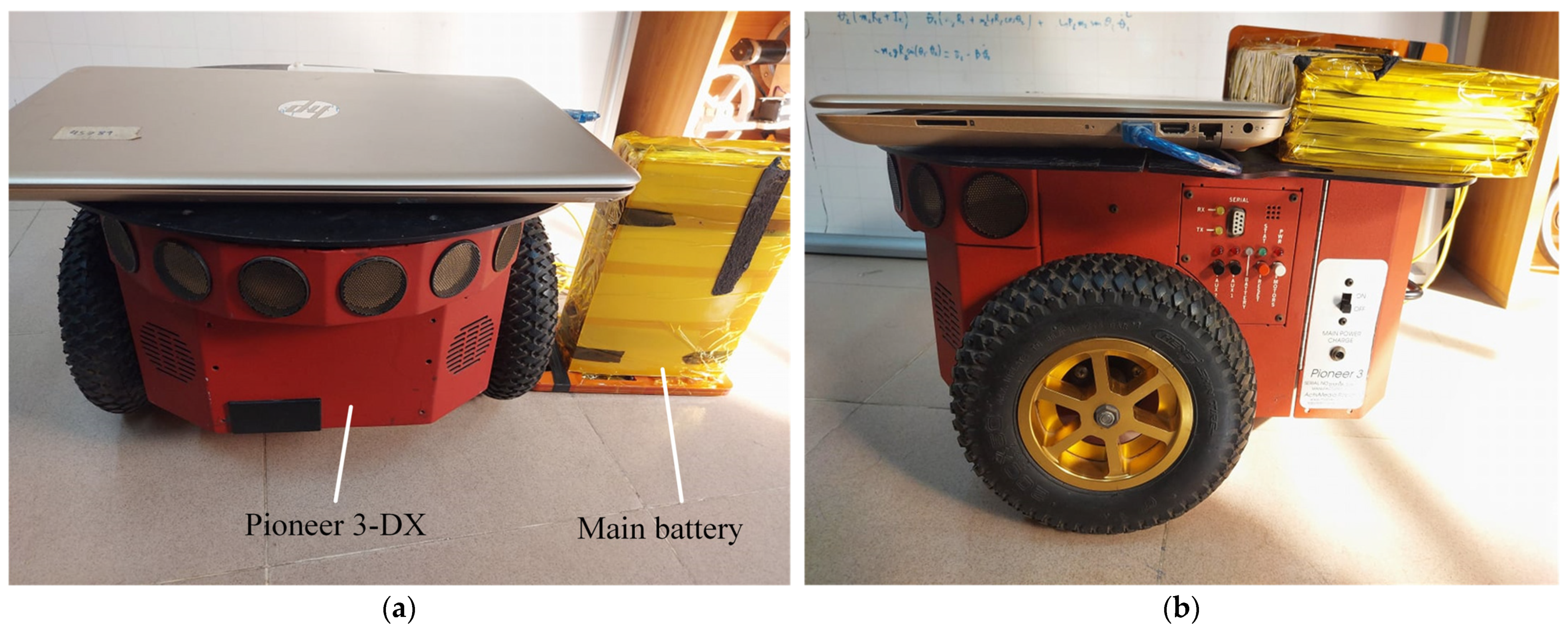
3.2. Experimental Scenario

The experiment is performed on a commercialized mobile robot named Pioneer 3-DX (P3-DX) (Figure 3). Encoders are installed on DC motors to perceive the rotational speed of the wheels. The reference trajectories are generated by a virtual robot implemented on a personal computer (PC). The PC also implements the proposed controller by retrieving the perception of the encoders from a microcontroller board to establish the control input, which is sent to the microcontroller board. The proposed controller’s control input becomes the reference input of a low-level speed controller for DC motors, implemented on the microcontroller board and known as inner loop control, which ensures the velocities of two wheels tracking to the control input of the proposed controller. Currently, the connection between the PC and the microcontroller board is serial communication with RS232 protocol, meaning that the baud rate is limited to 115,200 kbps. Further, wireless communication using either Long Range Radio (LoRa) technology or a well-known Wi-Fi ESP8266 also limits the bandwidth. Thus, the traveling interval and the data packet size of the communication should be reduced to save bandwidth. The specifications of P3-DX are shown in Table 2, below. A brief structure diagram of the mobile robot is also shown in Figure 4.

3.2.1. Event-Triggered Scenario

The parameters for the experiment are the same as those shown in Table 1. The mobile robot is required to move in a circular trajectory in 600 s, which means twenty laps of the circle with a radius of 0.5   m . The initial positions and estimated parameters of the mobile robot are x = 0.4   m and y = 0   m ; a ^ = 13 and b ^ = 1 . The controller gains are selected as k = 0.8 ,   γ 1 = 2 ,   γ 2 = 1.5 .

3.2.2. Time-Triggered Scenario

For an intuitive comparison, an experiment utilizing a time-triggered scheme instead of the event-triggered scheme is performed. Regarding the experiment conditions, the same test conditions of the event-triggered scenario are applied, except for the initial value of the estimated parameter a ^ which is a ^ = 1 in this case.

4. Results and Discussion

In general, the simulation and experimental results show that the response of the mobile robot under the control of the proposed controller has tracked the reference trajectory well for all scenarios, as shown in Figure 5. However, the spending time of the mobile robot to track the reference trajectories depends on the initial positions of the mobile robot. It is noted that the trajectory tracking of the mobile robot was more difficult at the vertices of the ellipse, shown in Figure 5b, than those of the circle, as shown in Figure 5a. The explanation for this phenomenon is that the ellipse trajectory possesses abrupt changes in velocities; however, the proposed controller is derived from a kinematic model, and such a controller can only perform well for a trajectory with almost linear velocities. Regarding the experimental results, it can be seen that the event-triggered scenario (Figure 5c) has a larger error boundary and a slower convergence rate than the time-triggered scenario (Figure 5d). This deviation is attributed to the continuous update of the control signal of the time-based update as opposed to the event-based update.
From Figure 6, it can be seen that the errors of X and Y in all scenarios are bounded despite existing fluctuations. The convergence rate can also be accelerated by choosing a higher gain k . However, the chattering phenomenon will worsen over time and ultimately degrade the control performance. In Figure 6a, the error of X reaches a peak at around 28 s. The same situation can also be seen in Figure 6b,c, albeit to a lesser extent. This can be attributed to the fact that during the first lap (0–30 s), the trajectory tracking of the mobile robot is still considered to be in the transient phase where the controller is adapting to the trajectory, and overshoot may occur as a result. Additionally, the use of pseudo-inverse in the matrix calculation of Equation (11) may cause some abnormalities depending on the simulation platform in some cases. As for the event-triggered and time-triggered experiments, the chattering effect is less prominent in the latter. Furthermore, the overshoots in transient time are lower in both the X and Y errors for the time-triggered scenario than those of the event-triggered scenario.
The angular error evolutions are depicted in Figure 7. Overall, all errors converge to zero after the first 30 s. It can be seen that the overshoot in the transient time of the case shown in Figure 7a is lower than those of the cases shown in Figure 7c,d. This can be explained by the fact that the simulation did not account for the weights of the PC and battery installed on the mobile robot. This leads to an increase in the inertia of moment in the actual robot, causing large overshoot. Moreover, the choice of the initial positions of the mobile robot affects the overshoot as well as the convergence time of the response. For instance, a larger initial value of b ^ for the case of the ellipse trajectory, shown in Figure 7b, can cause a more considerable overshoot than that of the circular trajectory, shown in Figure 7a; however, the convergence time of the former is faster.
Figure 8 shows that the chattering phenomenon affects the control signals v and ω . In general, the chattering phenomenon is much more prominent for the cases shown in Figure 8a,b than for the cases shown in Figure 8c, d, due to the amplitude of the reference velocities. In order to reduce the chattering effect, a saturation function can be implemented in place of the sign function or by implementing an advanced sliding mode controller such as high-order sliding mode and super-twisting sliding mode. Again, the velocities of the mobile robot under the control of the event-triggered scheme (Figure 8c) chatter more heavily than those controlled by the time-triggered scheme (Figure 8d). One reason is that the time interval between each update of the control input in the event-triggered case is higher, which causes a more significant error between each update and amplifies the chattering effect.
On the subject of estimating the parameters, the goal of the adaptive parameter scheme is to ensure that the estimated parameters are bounded and stable. In both the simulation and experimental results, the estimated parameters remained bounded, as shown in Figure 9. The responses of the parameters in the transient time are affected by the choice of the gains γ 1 and γ 2 ; instability for the estimated parameters will occur if the gains are chosen too high.
As for the triggering time, Figure 10 shows the time interval when the event is triggered, which is represented by pulse signals. Overall, the performances of the simulations and the experiment are nearly identical because the choice of the triggering threshold is the same. In the simulation, with the sampling time of 0.01 s, it can be calculated that the control input has to be updated 30,000 times, as shown in Figure 10a and Figure 10b, respectively. However, the implementation of the event-triggered strategy has reduced the times needed for updating to 12,050 and 17,070 times, which is significantly lower (accounting for 40% and 56.9% of the original). For the event-triggered experimental result, the control input for the event-triggered strategy is generated and updated 41,280 times in comparison with 60,000 times of the traditional controller, accounting for 68.8% of the total update intervals. This can be considered the advantage of the event-triggered strategy because it helped save computing resources.
The inter-event time denoted in plus signs for scenario 1, scenario 2, and the experiment is also shown in Figure 11. The efficiency of saving computing resources can be investigated through the inter-event time, with a high value signifying the system is not required to update for a long time, thus reducing frequent control computation. In general, the lowest inter-event time is 0.01 s for all cases. The inter-event time can reach up to 0.06 s and 0.1 s, as shown in Figure 11a and Figure 11b, respectively. In the event-triggered experiment shown in Figure 11c, 0.12 s is the highest inter-event time but it only occurs once, whereas the averages are 0.03 s, 0.02 s, and 0.01 s. In contrast, the inter-event time for the time-triggered experiment is always 0.01 s, as shown in Figure 11d, as the control input is updated at a fixed time interval.
To improve the inter-event time and reduce the number of triggered events, we can increase the threshold value for the triggering rule at the cost of precision. If the threshold value is sufficiently large, the control signals may not be updated for a long time, leading to the system’s instability as the controller cannot react quickly enough to drive the states’ errors to zero. On the contrary, a lower threshold means the computations of the control signals are more frequent, thus the states’ errors may not have any difficulty in converging to zero.

5. Conclusions

This paper presented a parameter-adaptive event-triggered sliding mode controller for a mobile robot. While the sliding mode controller drives the state variables to zero, the event-triggered scheme reduces the time needed for the microcontroller to calculate control input, thus saving resources. To further improve the accuracy of the controller, the adaptive method is also utilized to estimate the unknown physical parameters of the mobile robot. Simulations and experiments are performed to verify the effectiveness of the proposed controller in terms of errors and stability. Despite the tracking error convergence to zero, the control system is affected by the chattering phenomenon, and the convergence rate is still not optimized. In future work, these issues will be considered by utilizing an improved version of the sliding mode algorithm, such as a super-twisting algorithm. Additionally, the implementation of the proposed controller for a network control scheme using a standard messaging protocol in the application layer of the TCP/IP model, such as Message Queuing Telemetry Transport (MQTT), will be an interesting topic.

Author Contributions

Conceptualization, V.T.D.; methodology, T.D.T. and V.T.D.; software, T.D.T.; validation, V.T.D.; formal analysis, H.H.N.; investigation, T.D.T.; resources, T.T.N. (Trong Trung Nguyen) and T.T.N. (Tan Tien Nguyen); data curation, T.T.N. (Trong Trung Nguyen) and H.H.N.; writing—original draft preparation, T.D.T.; writing—review and editing, T.D.T. and V.T.D.; visualization, T.D.T. and T.T.N. (Trong Trung Nguyen); supervision, T.T.N. (Tan Tien Nguyen); project administration, T.T.N. (Tan Tien Nguyen); funding acquisition, T.T.N. (Tan Tien Nguyen). All authors have read and agreed to the published version of the manuscript.

Funding

This research was funded by Vietnam National University Ho Chi Minh City (VNU-HCM) under grant number C2020-20b-01.

Institutional Review Board Statement

Not applicable.

Informed Consent Statement

Not applicable.

Data Availability Statement

Data sharing is not applicable to this article.

Acknowledgments

This research is funded by Vietnam National University Ho Chi Minh City (VNU-HCM) under grant number C2020-20b-01. We acknowledge the support of time and facilities from National Key Laboratory of Digital Control and System Engineering (DCSELab), Ho Chi Minh City University of Technology (HCMUT), VNU-HCM for this study.

Conflicts of Interest

The authors declare no conflict of interest.

References

  1. Meng, L.; Lin, Y.; Gu, H.; Xu, H.; Geng, L. A New Type of Small Underwater Robot for Small Scale Ocean Observation. In Proceedings of the 6th Annual IEEE International Conference on Cyber Technology in Automation, Control and Intelligent Systems, IEEE-CYBER 2016, Chengdu, China, 19–22 June 2016; pp. 152–156. [Google Scholar] [CrossRef]
  2. Khatib, O.; Yeh, X.; Brantner, G.; Soe, B.; Kim, B.; Ganguly, S.; Stuart, H.; Wang, S.; Cutkosky, M.; Edsinger, A.; et al. Ocean one: A robotic avatar for oceanic discovery. IEEE Robot. Autom. Mag. 2016, 23, 20–29. [Google Scholar] [CrossRef]
  3. Bevacqua, G.; Cacace, J.; Finzi, A.; Lippiello, V. Mixed-initiative planning and execution for multiple drones in search and rescue missions. Proc. Int. Conf. Autom. Plan. Sched. 2015, 25, 315–323. Available online: https://ojs.aaai.org/index.php/ICAPS/article/view/13700 (accessed on 3 May 2022).
  4. Ferriere, L.; Raucent, B.; Campion, G. Design of omnimobile robot wheels. In Proceedings of the IEEE International Conference on Robotics and Automation, Minneapolis, MN, USA, 22–28 April 1996; Volume 4, pp. 3664–3670. [Google Scholar] [CrossRef]
  5. Soto, M.; Nava, P.A.; Alvarado, L.E. Drone formation control system real-time path planning. Collect. Tech. Pap.–2007 AIAA InfoTech Aerosp. Conf. 2007, 1, 606–639. [Google Scholar] [CrossRef]
  6. Thrun, S.; Bennewitz, M.; Burgard, W.; Cremers, A.B.; Dellaert, F.; Fox, D.; Hahnel, D.; Rosenberg, C.; Roy, N.; Schulte, J.; et al. MINERVA: A second-generation museum tour-guide robot. In Proceedings of the IEEE International Conference on Robotics and Automation, Detroit, MI, USA, 10–15 May 1999; Volume 3, pp. 1999–2005. [Google Scholar] [CrossRef]
  7. Triebel, R.; Arras, K.; Alami, R.; Beyer, L.; Breuers, S.; Chatila, R.; Chetouani, M.; Cremers, D.; Evers, V.; Fiore, M.; et al. SPENCER: A socially aware service robot for passenger guidance and help in busy airports. Springer Tracts Adv. Robot. 2016, 113, 607–622. [Google Scholar] [CrossRef] [Green Version]
  8. Marder-Eppstein, E.; Berger, E.; Foote, T.; Gerkey, B.; Konolige, K. The office marathon: Robust navigation in an indoor office environment. In Proceedings of the IEEE International Conference on Robotics and Automation, Anchorage, AK, USA, 3–7 May 2010; pp. 300–307. [Google Scholar] [CrossRef]
  9. Kanda, T.; Shiomi, M.; Miyashita, Z.; Ishiguro, H.; Hagita, N. An affective guide robot in a shopping mall. In Proceedings of the 4th ACM/IEEE International Conference on Human-Robot Interaction, HRI’09, La Jolla, CA, USA, 9 March 2008; pp. 173–180. [Google Scholar] [CrossRef] [Green Version]
  10. Kanayama, Y.; Miyazaki, F.; Kimura, Y.; Noguchi, T. A Stable Tracking Control Method for a Non-Holonomic Mobile Robot. Appl. Opt. 1991, 30, 523–530. [Google Scholar]
  11. Nakamura, Y.; Savant, S. Nonholonomic motion control of an autonomous underwater vehicle. In Proceedings of the IROS ’91:IEEE/RSJ International Workshop on Intelligent Robots and Systems ’91, Osaka, Japan, 3–5 November 2002; pp. 1254–1259. [Google Scholar] [CrossRef]
  12. Samson, C.; Ait-Abderrahim, K. Feedback control of a nonholonomic wheeled cart in Cartesian space. In Proceedings of the IEEE International Conference on Robotics and Automation, Sacramento, CA, USA, 9–11 April 1991; Volume 2, pp. 1136–1141. [Google Scholar] [CrossRef]
  13. Sampei, M.; Tamura, T.; Itoh, T.; Nakamichi, M. Path tracking control of trailer-like mobile robot. IROS 1992, 91, 193–198. [Google Scholar] [CrossRef]
  14. Fierro, R.; Lewis, F.L. Control of a nonholonomic mobile robot: Backstepping kinematics into dynamics. In Proceedings of the 1995 34th IEEE Conference on Decision and Control, New Orleans, LA, USA, 13–15 December 1995; Volume 4, pp. 3805–3810. [Google Scholar] [CrossRef]
  15. Shih, C.L.; Lin, L.C. Trajectory planning and tracking control of a differential-drive mobile robot in a picture drawing application. Robotics 2017, 6, 17. [Google Scholar] [CrossRef] [Green Version]
  16. Chang, Y.C.; Chen, B. Sen Adaptive tracking control design of nonholonomic mechanical systems. In Proceedings of the 35th IEEE Conference on Decision and Control, Kobe, Japan, 13 December 1996; Volume 4, pp. 4739–4744. [Google Scholar] [CrossRef]
  17. Gusev, S.V.; Makarov, I.A.; Paromtchik, I.E.; Yakubovich, V.A.; Laugier, C. Adaptive motion control of a nonholonomic vehicle. Proc.–IEEE Int. Conf. Robot. Autom. 1998, 4, 3285–3290. [Google Scholar] [CrossRef]
  18. Unluturk, A.; Aydogdu, O. Adaptive control of two-wheeled mobile balance robot capable to adapt different surfaces using a novel artificial neural network-based real-time switching dynamic controller. Int. J. Adv. Robot. Syst. 2017, 14, 1729881417700893. [Google Scholar] [CrossRef]
  19. Dengler, C.; Lohmann, B. Adjustable and adaptive control for an unstable mobile robot using imitation learning with trajectory optimization. Robotics 2020, 9, 29. [Google Scholar] [CrossRef]
  20. Gómez Ortega, J.; Camacho, E.F. Mobile robot navigation in a partially structured static environment, using neural predictive control. Control Eng. Pract. 1996, 4, 1669–1679. [Google Scholar] [CrossRef]
  21. Zhang, T.; Kahn, G.; Levine, S.; Abbeel, P. Learning deep control policies for autonomous aerial vehicles with MPC-guided policy search. In Proceedings of the 2016 IEEE International Conference on Robotics and Automation (ICRA), Stockholm, Sweden, 16–21 May 2016; Volume 2016, pp. 528–535. [Google Scholar] [CrossRef] [Green Version]
  22. Fukao, T.; Nakagawa, H.; Adachi, N. Adaptive tracking control of a nonholonomic mobile robot. IEEE Trans. Robot. Autom. 2000, 16, 609–615. [Google Scholar] [CrossRef]
  23. Goodwin, G.C.; Aguero, J.C.; Cea Garridos, M.E.; Salgado, M.E.; Yuz, J.I. Sampling and sampled-data models: The interface between the continuous world and digital algorithms. IEEE Control Syst. 2013, 33, 34–53. [Google Scholar] [CrossRef]
  24. Nowzari, C.; Garcia, E.; Cortés, J. Event-triggered communication and control of networked systems for multi-agent consensus. Automatica 2019, 105, 1–27. [Google Scholar] [CrossRef] [Green Version]
  25. Jiang, Z.P.; Liu, T.F. A survey of recent results in quantized and event-based nonlinear control. Int. J. Autom. Comput. 2015, 12, 455–466. [Google Scholar] [CrossRef] [Green Version]
  26. Johan Åström, K.; Bernhardsson, B. Comparison of Periodic and Event Based Sampling for First–Order Stochastic Systems. IFAC Proc. Vol. 1999, 32, 5006–5011. [Google Scholar] [CrossRef] [Green Version]
  27. Tabuada, P. Event-triggered real-time scheduling of stabilizing control tasks. IEEE Trans. Automat. Control 2007, 52, 1680–1685. [Google Scholar] [CrossRef] [Green Version]
  28. Henningsson, T.; Johannesson, E.; Cervin, A. Sporadic event-based control of first-order linear stochastic systems. Automatica 2008, 44, 2890–2895. [Google Scholar] [CrossRef]
  29. Zietkiewicz, J.; Horla, D.; Owczarkowski, A. Sparse in the time stabilization of a bicycle robot model: Strategies for event- and self-triggered control approaches. Robotics 2018, 7, 77. [Google Scholar] [CrossRef] [Green Version]
  30. González, A.; Cuenca, Á.; Salt, J.; Jacobs, J. Robust stability analysis of an energy-efficient control in a Networked Control System with application to unmanned ground vehicles. Inf. Sci. 2021, 578, 64–84. [Google Scholar] [CrossRef]
  31. Du, S.; Yan, Q.; Qiao, J. Event-triggered PID control for wastewater treatment plants. J. Water Process Eng. 2020, 38, 101659. [Google Scholar] [CrossRef]
  32. Wu, J.; Peng, C. Observer-based adaptive event-triggered PID control for networked systems under aperiodic DoS attacks. Int. J. Robust Nonlinear Control 2022, 32, 2536–2550. [Google Scholar] [CrossRef]
  33. Heemels, W.P.M.H.; Sandee, J.H.; Van Den Bosch, P.P.J. Analysis of event-driven controllers for linear systems. Int. J. Control 2008, 81, 571–590. [Google Scholar] [CrossRef]
  34. Wang, X.; Lemmon, M.D. Event-triggering in distributed networked control systems. IEEE Trans. Automat. Control 2011, 56, 586–601. [Google Scholar] [CrossRef] [Green Version]
  35. Heemels, W.P.M.H.; Donkers, M.C.F.; Teel, A.R. Periodic event-triggered control for linear systems. IEEE Trans. Automat. Control 2013, 58, 847–861. [Google Scholar] [CrossRef]
  36. Singh, P.; Agrawal, P.; Nandanwar, A.; Behera, L.; Verma, N.K.; Nahavandi, S.; Jamshidi, M. Multivariable Event-Triggered Generalized Super-Twisting Controller for Safe Navigation of Nonholonomic Mobile Robot. IEEE Syst. J. 2021, 15, 454–465. [Google Scholar] [CrossRef]
  37. Yan, Y.; Yu, S.; Sun, C. Event-triggered sliding mode tracking control of autonomous surface vehicles. J. Franklin Inst. 2021, 358, 4393–4409. [Google Scholar] [CrossRef]
  38. Nafia, N.; El Kari, A.; Ayad, H.; Mjahed, M. Robust interval type-2 fuzzy sliding mode control design for robot manipulators. Robotics 2018, 7, 40. [Google Scholar] [CrossRef] [Green Version]
  39. Hu, Y.; Su, H.; Zhang, L.; Miao, S.; Chen, G.; Knoll, A. Nonlinear model predictive control for mobile robot using varying-parameter convergent differential neural network. Robotics 2019, 8, 64. [Google Scholar] [CrossRef] [Green Version]
  40. Bozek, P.; Karavaev, Y.L.; Ardentov, A.A.; Yefremov, K.S. Neural network control of a wheeled mobile robot based on optimal trajectories. Int. J. Adv. Robot. Syst. 2020, 17, 1729881420916077. [Google Scholar] [CrossRef] [Green Version]
  41. Zou, A.M.; Hou, Z.G.; Fu, S.Y.; Tan, M. Neural networks for mobile robot navigation: A survey. Lect. Notes Comput. Sci. 2006, 3972, 1218–1226. [Google Scholar] [CrossRef]
  42. Kaaniche, K.; Rashid, N.; Miraoui, I.; Mekki, H.; El-Hamrawy, O.I. Mobile Robot Control Based on 2D Visual Servoing: A New Approach Combining Neural Network with Variable Structure and Flatness Theory. IEEE Access 2021, 9, 83688–83694. [Google Scholar] [CrossRef]
  43. Oryschuk, P.; Salerno, A.; Al-Husseini, A.M.; Angeles, J. Experimental validation of an underactuated two-wheeled mobile robot. IEEE/ASME Trans. Mechatron. 2009, 14, 252–257. [Google Scholar] [CrossRef]
  44. Lang, H.; Wang, Y.; De Silva, C.W. Visual servoing with LQR control for mobile robots. In Proceedings of the 2010 8th IEEE International Conference on Control and Automation, Xiamen, China, 9–11 June 2010; pp. 317–321. [Google Scholar] [CrossRef]
  45. Duong, V.T.; Nguyen, D.T.; Luu, Q.L.; Nguyen, T.T.; Nguyen, H.H.; Nguyen, T.T. Indoor Virtual Path Tracking for Mobile Robot using Sensor Fusion by Extended Kalman Filter. Int. J. Mech. Mechatron. Eng. 2020, 20, 104–110. [Google Scholar]
  46. Nath, K.; Yesmin, A.; Nanda, A.; Bera, M.K. Event-Triggered Sliding-Mode Control of Two Wheeled Mobile Robot: An Experimental Validation. IEEE J. Emerg. Sel. Top. Ind. Electron. 2021, 2, 218–226. [Google Scholar] [CrossRef]
  47. Van, M.; Mavrovouniotis, M.; Ge, S.S. An adaptive backstepping nonsingular fast terminal sliding mode control for robust fault tolerant control of robot manipulators. IEEE Trans. Syst. Man Cybern. Syst. 2019, 49, 1448–1458. [Google Scholar] [CrossRef] [Green Version]
  48. Chen, H.; Zhang, B.; Zhao, T.; Wang, T.; Li, K. Finite-time tracking control for extended nonholonomic chained-form systems with parametric uncertainty and external disturbance. J. Vib. Control 2018, 24, 100–109. [Google Scholar] [CrossRef] [Green Version]
  49. Mu, J.; Yan, X.G.; Spurgeon, S.K.; Mao, Z. Generalized Regular Form Based SMC for Nonlinear Systems with Application to a WMR. IEEE Trans. Ind. Electron. 2017, 64, 6714–6723. [Google Scholar] [CrossRef] [Green Version]
  50. Yu, H.; Chen, T. On Zeno Behavior in Event-Triggered Finite-Time Consensus of Multiagent Systems. IEEE Trans. Automat. Control 2021, 66, 4700–4714. [Google Scholar] [CrossRef]
  51. Xing, L.; Wen, C.; Liu, Z.; Su, H.; Cai, J. Event-triggered adaptive control for a class of uncertain nonlinear systems. IEEE Trans. Automat. Control 2017, 62, 2071–2076. [Google Scholar] [CrossRef]
  52. Huang, J.; Wang, W.; Wen, C.; Li, G. Adaptive Event-Triggered Control of Nonlinear Systems with Controller and Parameter Estimator Triggering. IEEE Trans. Automat. Control 2020, 65, 318–324. [Google Scholar] [CrossRef]
Figure 1. Model of a mobile robot: (a) kinematic model; (b) mobile robot and virtual robot.
Robotics 11 00078 g001
Figure 2. Block diagram of the mobile robot’s system.
Robotics 11 00078 g002
Figure 3. Front and side view of P3-DX: (a) front view; (b) side view with battery attached on top.
Robotics 11 00078 g003
Figure 4. Structure diagram of the mobile robot.
Robotics 11 00078 g004
Figure 5. Trajectory tracking of the mobile robot: (a) circular trajectory (simulation); (b) ellipse trajectory (simulation); (c) circular trajectory—event-triggered (experiment); (d) circular trajectory—time-triggered (experiment).
Robotics 11 00078 g005aRobotics 11 00078 g005b
Figure 6. X and Y coordinates’ errors: (a) circular trajectory (simulation); (b) ellipse trajectory (simulation); (c) circular trajectory—event-triggered (experiment); (d) circular trajectory—time-triggered (experiment).
Robotics 11 00078 g006aRobotics 11 00078 g006b
Figure 7. Angular errors: (a) circular trajectory (simulation); (b) ellipse trajectory (simulation); (c) circular trajectory—event-triggered (experiment); (d) circular trajectory—time-triggered (experiment).
Robotics 11 00078 g007
Figure 8. Linear and angular velocities: (a) circular trajectory (simulation); (b) ellipse trajectory (simulation); (c) circular trajectory—event-triggered (experiment); (d) circular trajectory—time-triggered (experiment).
Robotics 11 00078 g008
Figure 9. Estimated parameter evolution: (a) circular trajectory (simulation); (b) ellipse trajectory (simulation); (c) circular trajectory—event-triggered (experiment); (d) circular trajectory—time-triggered (experiment).
Robotics 11 00078 g009
Figure 10. Triggered event in the first 10 s: (a) circular trajectory (simulation); (b) ellipse trajectory (simulation); (c) circular trajectory—event-triggered (experiment); (d) circular trajectory—time-triggered (experiment).
Robotics 11 00078 g010
Figure 11. Inter-event time versus time: triggered events in the first 10 s. (a) Circular trajectory (simulation); (b) ellipse trajectory (simulation); (c) circular trajectory—event-triggered (experiment); (d) circular trajectory—time-triggered (experiment).
Robotics 11 00078 g011aRobotics 11 00078 g011b
Table 1. Simulation parameters.
ParametersValueParametersValue
Sampling time 0.01 s η ¯ 1.5
a 10.5 L 1 0.3
b 1.74 L 2 0.45
Initial value of a 8 L 170
Initial value of b 1 μ 0.5
δ ¯ 1.2
Table 2. P3-DX specifications.
Dimensions (L × W × H) (mm) 455 × 381 × 237
Total weight 9   kg
Maximum load capacity 17   kg
Maximum velocity 1.2   m / s
Maximum acceleration 2   m / s 2
Main actuatorsPITTMAN GM9236
Publisher’s Note: MDPI stays neutral with regard to jurisdictional claims in published maps and institutional affiliations.

