Quantum Rainbows in Positron Transmission through Carbon Nanotubes

Abstract

Here we report the results of the theoretical investigation of the transmission of channeled positrons through various short chiral single walled carbon nanotubes (SWCNT). The main question answered by this study is “What are the manifestations of the rainbow effect in the channeling of quantum particles that happens during the channeling of classical particles?” To answer this question, the corresponding classical and quantum problems were solved in parallel, critically examined, and compared with each other. Positron energies were taken to be 1 MeV when the quantum approach was necessary. The continuum positron-nanotube potential was constructed from the thermally averaged Molière’s positron-carbon potential. In the classical approach, a positron beam is considered as an ensemble of noninteracting particles. In the quantum approach, it is considered as an ensemble of noninteracting wave packages. Distributions of transmitted positrons were constructed from the numerical solutions of Newton’s equation and the time-dependent Schrödinger equation. For the transmission of 1-MeV positrons through 200-nm long SWCNT (14; 4), in addition to the central maximum, the quantum angular distribution has a prominent peak pair (close to the classical rainbows) and two smaller peaks pairs. We have shown that even though the semiclassical approximation is not strictly applicable it is useful for explanation of the observed behavior. In vicinity of the most prominent peak, i.e., the primary rainbow peak, rays interfere constructively. On one of its sides, rays become complex, which explains the exponential decay of the probability density in that region. On the other side, the ray interference alternates between constructive and destructive, thus generating two observed supernumerary rainbow peaks. The developed model was then applied for the explanation of the angular distributions of 1-MeV positrons transmitting through 200 nm long (7, 3), (8, 5), (9, 7), (14, 4), (16, 5) and (17, 7) SWCNTs. It has been shown that this explains most but not all rainbow patterns. Therefore, a new method for the identification and classification of quantum rainbows was developed relying only on the morphological properties of the positron wave function amplitude and the phase function families. This led to a detailed explanation of the way the quantum rainbows are generated. All wave packets wrinkle due to their internal focusing in a mutually coordinated way and are concentrated near the position of the corresponding classical rainbow. This explanation is general and applicable to the investigations of quantum effects occurring in various other atomic collision processes.

1. Introduction

Let us consider a single perfect graphene sheet shown in the Figure 1a. The primitive vectors of the graphene lattice are denoted as ${\mathit{a}}_{\mathbf{1}}$, and ${\mathit{a}}_{\mathbf{2}}$. Single wall carbon nanotubes (SWCNTs) can be seen as a graphene sheet rolled-up to form a cylinder [1]. However, rolling up of the graphene sheet is possible only in certain directions. To form a nanotube it is necessary that its circumference be equal to the length of the vector, called the chiral vector ${\mathit{C}}_{\mathit{h}}=m{\mathit{a}}_{\mathbf{1}}+n{\mathit{a}}_{\mathbf{2}}$ specifying possible distances between atoms of the sheet. The resulting SWCNT is made of the infinite number of nanotube unit cells containing N carbon atoms translationally repeating itself in the direction orthogonal to the vector ${\mathit{C}}_{\mathit{h}}$, defining the nanotube axis. Chiral indices $(m,n)$ uniquely determine the structure of nanotube [1], and are used for the identification of the nanotubes. Depending on the direction of the vector ${\mathit{C}}_{\mathit{h}}$, all SWCNTs can be classified in the three classes: zig-zag ${\mathit{C}}_{\mathit{h}}=(0,n)$, armchair ${\mathit{C}}_{\mathit{h}}=(n,n)$, and generic nanotubes also called chiral ${\mathit{C}}_{\mathit{h}}=(m,n)$. Views in the direction of the axis of the zig-zag, armchair, and chiral SWCNT are shown in the Figure 1a–c, respectively. Nanotubes have extraordinary elastic, electronic and thermal properties. A good overview of nanotube properties which are important for the potential applications can be found in the references [2,3,4].

Viewed in the direction of their axes, SWCNTs can be described as an arrangement of atomic strings (see Figure 1b–d). Let us now examine the scattering of a positively charged particle by an atomic string. A schematic representation of this process is shown in Figure 2a. If the positively charged particle is directed towards the atomic string at a small angle, then it will be reflected back by the correlated series of small angle scatterings on atoms of the string. The particle does not fall under the influence of individual atoms, rather it behaves as if being scattered by the atomic string itself. To deflect the particle trajectory, the potential energy of the atomic string U, at the distance of the closest approach, must be equal to the particle transverse kinetic energy. Lindhard has shown that minimal approach distance is approximately equal to the atom screening radius $a_{\mathrm{sc}}$ [5]. Consequently, the maximal incident angle ${\Theta }_c$, called the critical angle, is defined by relation

$${\Theta }_c\approx \sqrt{\frac{U(a_{\mathrm{sc}})}{E_k}},$$

(1)

where $E_k$ is the kinetic energy of the incoming particle.

Figure 2b show the schematic representation of the particle bounded motion in the potential of the SWCNT. Such a motion occurs if the angle between SWCNT axis and ion velocity vector in the entrance plane of the nanotube is smaller than ${\Theta }_c$. The subsequent series of scatterings by atomic strings then gently guides the particle trajectory through the regions of low electron density. At all times an angle measuring the deflection of the particle from the SWCNT axis remains small. The described mode of particle motion is called channeling.

Nanotubes were discovered in 1991 by Iijima [6]. Soon after their discovery, Klimov and Letokhov demonstrated that SWCNT can be used for the channeling of positively charged particles [7]. The same authors predicted that the motion of channeled particles would generate X-ray and $\gamma$-ray radiation [7,8]. A lot of subsequent studies were devoted to the investigation of the possibility to use nanotube for ion guiding and the construction of nanotube based undulators. A good review devoted to particle channeling in the SWCNT can be found in the Ref. [9].

Rainbow scattering occurs if the neighboring sections of the impact parameter plane are scattered to the same section of the scattering angle plane. As a consequence, the differential cross-section becomes infinite along certain lines, called rainbows. The best-known example of the rainbow scattering is the scattering of the light rays by the droplet of water generating the meteorological rainbow [10]. Rainbow scattering happens in nucleus-nucleus collisions [11], elastic scattering [12], electron-molecule collisions [13], particle scattering form the surfaces [14], and ion channeling in crystals [15].

Petrović et al. have shown that the rainbow effect appears also in ion channeling through SWCNTs [16]. It was shown that the theory of rainbows, developed for the explanation of the rainbow channeling in crystals [17], can also be applied for the explanation of the most important features of the rainbow channeling in SWCNTs. A summary of the most important findings of the mentioned group can be found in the Ref. [18].

Besides its theoretical significance, the rainbow effect has a number of practical uses. It was used to extract the correct proton-Si interaction potential [19], and there is also suggestion to be employed for production of the ion beams focused to the subatomic precision [20]. A new method for characterization of the short SWCNTs proposed in the Refs. [21,22] is based on the rainbow effect. It has been shown that the quantum rainbow channeling effect is even more sensitive to the variation of the SWCNT radius [23,24]. Therefore, it is reasonable to expect that quantum rainbow channeling is useful for investigation of the nanotubes and other nanostructured materials.

It should be noted that the classical approach is usually sufficient for the description of the channeling effects of energetic charged particles. Recently, Takabayashi et al. reported on the first experimental observation of the rainbow effect in the planar channeling of 1GeV electrons in the Si crystal [25]. In their experiments, no wave-features of the transmitted electron beam were observed. According to the classical theory, the density of ion trajectories on the rainbow line is infinite. The classical particle density is a strictly additive quantity; therefore, on the rainbow line it is also infinite. However, any particle also behaves as a wave. Due to the interference individual contributions to the wave function amplitude of the wave trains moving approximately along the classical trajectories can be additive or subtractive. The net result is a finite particle density of the rainbow peak, and in a number of additional smaller peaks called supernumerary rainbows. Therefore, even for classical particles it is not possible to understand the true nature of the rainbow effect without quantum mechanics. However, for particles of high energy, the rainbow pattern is so fine that it is difficult to observe it even using detectors of very high resolution.

For light particles whose energies are in the MeV range the quantum description becomes mandatory. Recent theoretical publications of the Kharkov group were devoted to the investigation of the quantum rainbow channeling of electrons in ultra-thin crystals [26,27]. They explained observed wave features as a result of the electron diffraction on the periodic arrangement of the atomic planes or strings. They did not provide any finer classification of the rainbow peaks. Schüller and Winter experimentally observed supernumerary rainbows in scattering of fast atoms by the LiF(001) surface [28]. Their interpretation of the results was based on the semiclassical approach.

The problem of the form of the quantum wave function in the vicinity of the rainbow line and classification of rainbow peaks is well known. It is usually treated in the framework of the semiclassical approach employing uniform approximation [11,29]. However, this approach is applicable only when longitudinal energy is so large that asymptotic approximations are applicable [30]. Another approach is to treat the motion of quantum channeled particles using the formalism of dynamical diffraction [31,32,33,34]. However, expanding the incoming wave function in the Bloch state basis is unable to describe the propagation of the evanescent waves, which are shown to be important for the description of the interference in the vicinity of the rainbow line [35]. It is in principle possible to introduce complex interaction potentials which would generate, required imaginary branches of the dispersion relations, but it is difficult to obtain parametrization of such a potential which reproduces observable results. In both approaches, the incoming particle beam is represented as a plane wave. This assumption is perfectly adequate for the description of the wave diffraction. However, there are two main reasons why this is not desirable in particle channeling. Firstly, with simple plane wave it is difficult to model the influence of the beam divergence on the resulting distributions. Angular divergence is extremely important quantity. If it is larger than the critical angle ${\Theta }_c$ then there is no channeling at all. Secondly, the plane wave is infinite, it interacts with the whole sample at the same time. The experimentally proven characteristic feature of the channeling effect is that all physical quantities (such as energy loss, dechanneling probability, etc.) are orientational and impact parameter dependent. This means that one needs to consider fine details of the individual scattered waves. Using the plane wave, one immediately gets a wave describing the interference of all scattered waves and such detailed investigation is impossible. Also, it has been found that the difference between angular distributions of the transmitted parallel positron beam represented as the plane wave and diverging beam represented as an ensemble of wave packets can be large (compare Figure 4 against Figures 7 and 8 of the Ref. [23]).

The simplest way to remedy all the mentioned drawbacks is to represent particles as wave packets and to base the analysis on the explicit solution of the time dependent Schödinger equation. In this report, the transmission of 1-MeV positrons will be examined in detail, when quantum treatment is needed. Initially, quantum particles will be represented as Gaussian wave packets. The corresponding classical problem will be examined in parallel, and both results will be compared and critically examined. We start with a brief review of the classical rainbow channeling theory, and give a short description of the developed model of quantum channeling. Next, we show how to interpret obtained exact solutions using the language of the semiclassical approach. At the end, we present a method for classification of prominent peaks of transmitted distributions relaying only on the information contained in the corresponding quantum amplitude and phase functions families.

2. Theory

In this section, a brief review of the theory of rainbow channeling will be given, and a model of quantum rainbow channeling will be presented. The z axis of the adopted coordinate system is aligned with the axis of the nanotube. The x and y axes are vertical and horizontal axes, respectively.

2.1. Interaction Potential

The primitive vectors of the graphene lattice are denoted as ${\mathit{a}}_{\mathbf{1}}$, and ${\mathit{a}}_{\mathbf{2}}$. Their lengths are $|{\mathit{a}}_{\mathbf{1}}|=|{\mathit{a}}_{\mathbf{2}}|=\sqrt{3}l$, where $l=0.14$ nm stands for the carbon-carbon bond length. The angle between vectors is $\pi /3$. Chiral vector is defined by expression ${\mathit{C}}_{\mathit{h}}=m{\mathit{a}}_{\mathbf{1}}+n{\mathit{a}}_{\mathbf{2}}$. Consequently, the radius of the nanotube is given by the expression

$$R=\frac{|{\mathit{C}}_{\mathit{h}}|}{2\pi }=\frac{\sqrt{3}l}{2\pi }{\left(m^2+mn+n^2\right)}^{1/2},$$

(2)

and translational vector of SWCNT unit cell is

$$\mathit{T}=\frac{1}{q_{mn}}\left[(2n+m){\mathit{a}}_{\mathbf{1}}+(2m+n){\mathit{a}}_{\mathbf{2}}\right].$$

(3)

where $q_{mn}$ is the greatest common divisor of $2m+n$ and $2n+m$. The number of atoms in the SWCT unit cell

$$N=\frac{4}{q_{mn}}(m^2+nm+n^2)$$

(4)

is equal to the number of graphene atoms contained in a rectangle defined by vectors ${\mathit{C}}_{\mathit{h}}$, and $\mathit{T}$. Each atom is the starting point of one atomic string forming circumference of the SWCNT.

We assume that the potential describing charged particle carbon interaction is given by the Molière’s expression [36]

$$V(\overline{\mathit{r}})=\frac{Z_1{Z}_2{e}^2}{4\pi {\epsilon }_0|\overline{\mathit{r}}|}\sum _{k=1}^3{\alpha }_{k}exp\left[-{\beta }_k\frac{|\overline{\mathit{r}}|}{a_{\mathrm{sc}}}\right].$$

(5)

where $Z_1$, $Z_2$ are charge state of the incoming particle and carbon atomic number ($Z_2=6$), respectively; e is the elementary charge; $\overline{\mathit{r}}=(\overline{x},\overline{y},\overline{z})=\mathit{r}-{\mathit{r}}_o$ represent the distance vector between positions of the particle $\mathit{r}=(x,y,z)$, and carbon atom ${\mathit{r}}_o=(x_0,y_0,z_0)$; ${\epsilon }_0$ is dielectric permittivity of the vacuum; $a_{\mathrm{sc}}={[9{\pi }^2/(128Z_2)]}^{1/3}{a}_{\mathrm{B}}$ is Thomas-Fermi screening radius, while $a_{\mathrm{B}}$ is the Bohr’s radius; $\mathit{\alpha }=[0.35,0.55,0.10]$, and $\mathit{\beta }=[0.1,1.2,6.0]$ are Molière’s fitting parameters. The channeled particle does not feel the influence of the potential of individual atoms $V(\overline{\mathit{r}})$, rather, its trajectory is influenced by the longitudinally averaged atomic potential of the atomic string

$$U(\overline{\mathit{\rho }})=\frac{1}{|\mathit{T}|}\underset{-\infty }{\overset{\infty }{\int }}V(\overline{\mathit{r}})\mathrm{d}\overline{z}=\frac{Z_1{Z}_2{e}^2}{2\pi {\epsilon }_0|\mathit{T}|}\sum _{k=1}^3{\alpha }_k{K}_0\left({\beta }_k\frac{|\overline{\mathit{\rho }}|}{a_{\mathrm{sc}}}\right),$$

(6)

where $\overline{\mathit{\rho }}=(\overline{x},\overline{y})=\mathit{\rho }-{\mathit{\rho }}_{\mathit{o}}$ is distance vector between transverse positions of particle $\mathit{\rho }=(x,y)$, and atomic string ${\mathit{\rho }}_o=(x_0,y_0)$; $K_0$ is modified Bessel function of the second kind and 0-th order [37]. Potential of the SWCNT $U_{{\mathit{C}}_{\mathit{h}}}$ at the transverse point $\mathit{\rho }$ is the sum of contributions of all atomic strings located at transverse positions ${\mathit{\rho }}_s$ ($s=1,\dots ,N$). It can be shown that the potential $U_{{\mathit{C}}_{\mathit{h}}}$ is given by the expression [38]:

$$\begin{array}{ccc}\hfill U_{{\mathit{C}}_{\mathit{h}}}(\mathit{\rho };R)& =& {\displaystyle \sum _{s=1}^N}U(\mathit{\rho }-{\mathit{\rho }}_s)\hfill \\ & =& \frac{Z_1{Z}_2{e}^{2}R}{3\sqrt{3}{l}^2{\epsilon }_0}{\displaystyle \sum _{k=1}^3}\left[U_0^k(\rho ;R)+2{\displaystyle \sum _{\mu =1}^{\infty }}{U}_{\frac{\mu N}{2}}^k(\rho ;R)cos\left(\frac{\mu N}{2}\Delta \varphi \right)cos\left(\frac{\mu N}{2}(\varphi -\Delta \varphi )\right)\right],\hfill \end{array}$$

(7)

where $\rho$ and $\varphi$ are coordinates of the vector $\mathit{\rho }$ in polar coordinate system; $\Delta \varphi =(m+n)\pi /(2m^2+2mn+2n^2)$; while quantities $U_{\nu }^k(\rho )$ are defined by expression:

$$U_{\nu }^k(\rho ;R)=\left\{\begin{array}{ccc}\hfill {\alpha }_k{I}_{\nu }\left({\beta }_k\frac{\rho }{a_{\mathrm{sc}}}\right)K_{\nu }\left({\beta }_k\frac{R}{a_{\mathrm{sc}}}\right),& \mathrm{for}& \rho \le R,\hfill \\ \hfill {\alpha }_k{K}_{\nu }\left({\beta }_k\frac{\rho }{a_{\mathrm{sc}}}\right)I_{\nu }\left({\beta }_k\frac{R}{a_{\mathrm{sc}}}\right),& \mathrm{for}& \rho >R.\hfill \end{array}\right.$$

(8)

$I_{\nu }$, and $K_{\nu }$ are modified Bessel functions of the first and second kind and $\nu$-th order [37]. In channeling, thermal effects are introduced by averaging the static potential $U_{{\mathit{C}}_{\mathit{h}}}$ over the distribution of atoms thermal vibrations [38,39]

$$U_{{\mathit{C}}_{\mathit{h}}}^{th}(\mathit{\rho };R)={\int }_{{\mathit{\rho }}^{\prime }}{P}_{th}(\mathit{\rho }-{\mathit{\rho }}^{\prime })U_{{\mathit{C}}_{\mathit{h}}}({\mathit{\rho }}^{\prime };R)\mathrm{d}{\mathit{\rho }}^{\prime },$$

(9)

where $P_{th}(\mathit{\rho })=\frac{1}{\sqrt{{(2\pi )}^2|det\mathsf{\Sigma }|}}exp[-\frac{1}{2}{\mathit{\rho }}^T·{\mathsf{\Sigma }}^{-1}·\mathit{\rho }]$ is distribution of carbon transverse thermal motion; $\mathsf{\Sigma }$ is its associate covariance matrix; while ${\mathit{\rho }}^T$ is transposed vector.

2.2. Theory of Rainbow Channeling

For simplicity, we assume that the incoming particle beam is monochromatic, perfectly collimated and aligned with the nanotube axis. We also assume that the energy of the particle is sufficiently large so that the energy loss and fluctuation of the scattering angle due to the interaction with SWCNT electrons can be neglected. Once the interaction potential is known, the particle trajectories can be found by solving Newton’s equations of motion

$$m\frac{{\mathrm{d}}^2\mathit{r}}{\mathrm{d}{t}^2}=-\nabla U_{{\mathit{C}}_{\mathit{h}}}^{th}(\mathit{\rho };R),$$

(10)

where m is particle mass, t denotes the time, and $\nabla =({\partial }_x,{\partial }_y,{\partial }_z)$. Appropriate initial conditions are $\mathit{r}(t=0)=(\mathit{b},0)$, and $\mathit{v}=(0,0,v_z)$; $\mathit{b}=(b_x,b_y)$ is the particle impact parameter. The distribution of the incoming, macroscopic particle beam is uniform on the scale of the nanotube; therefore, the impact parameters $\mathit{b}$ should be random samples form uniform distribution. The Equation (10) shows that the motion of the particle in the longitudinal direction is free. It is inertial motion with constant velocity $v_z$, while motion in the transverse plane satisfies equation

$$m\frac{{\mathrm{d}}^2\mathit{\rho }}{\mathrm{d}{t}^2}=-\nabla U_{{\mathit{C}}_{\mathit{h}}}^{th}(\mathit{\rho };R).$$

(11)

Therefore, the particle trajectory can be parameterized by a value of the longitudinal coordinate z. At the exit of the SWCNT of length L, trajectory end point determines particle exit transverse position $\mathit{\rho }(L)$ and deflection angle $\mathit{\theta }=({\theta }_x,{\theta }_y)$ (see Figure 2b). Angular and spatial distributions of transmitted particles $Y_{\theta }$ and $Y_{\rho }$ are constructed by counting the number of particles detected at the specific angle and at the specific position. It should be noted that in principle spatial yield $Y_{\rho }$ is measurable. To observe it a position sensitive detector of picometer resolution is required, which still does not exist.

Particle trajectories define two mappings: a mapping of the impact parameter plane to the final transmission position plane $\mathit{b}\to \mathit{\rho }$, and a mapping of the impact parameter plane to the final transmission angle plane $\mathit{b}\to \mathit{\theta }$. Since the initial distribution of particles is uniform, the differential cross-sections describing scattering process are defined by the following expressions

$${\sigma }_{\mathrm{diff}}^{\rho }(\mathit{\rho })=\frac{\mathrm{d}{b}_x\mathrm{d}{b}_y}{\mathrm{d}x\mathrm{d}y}=\frac{1}{|J_r|},{\sigma }_{\mathrm{diff}}^{\theta }(\mathit{\theta })=\frac{\mathrm{d}{b}_x\mathrm{d}{b}_y}{\mathrm{d}{\theta }_x\mathrm{d}{\theta }_y}=\frac{1}{|J_{\theta }|},$$

(12)

where $J_{\rho }$ and $J_{\theta }$ are determinants of Jacobian matrices associated with mappings $\mathit{b}\to \mathit{\rho }$, and $\mathit{b}\to \mathit{\theta }$, respectively. Differential cross-sections are infinite whenever the following equations are satisfied.

$$J_{\rho }(\mathit{b})=\frac{\partial x}{\partial b_x}\frac{\partial y}{\partial b_y}-\frac{\partial x}{\partial b_y}\frac{\partial y}{\partial b_x}=0,J_{\theta }(\mathit{b})=\frac{\partial {\theta }_x}{\partial b_x}\frac{\partial {\theta }_y}{\partial b_y}-\frac{\partial {\theta }_x}{\partial b_y}\frac{\partial {\theta }_y}{\partial b_x}=0.$$

(13)

The solutions of Equations (13) form lines in the impact parameter plane, called spatial, and angular impact parameter rainbow lines, respectively. Their images obtained by the application of the corresponding mapping $\mathit{b}\to \mathit{\rho }$, and $\mathit{b}\to \mathit{\theta }$ respectively, are also lines, called spatial and angular rainbow lines, respectively. Note that spatial and angular rainbow lines separate areas of different multiplicities of the mappings $\mathit{\theta }\to \mathit{b}$, and $\mathit{\rho }\to \mathit{b}$. The side of higher multiplicity is called the bright side of the rainbow, while the rainbow side of lower multiplicity is called the dark side of the rainbow. Thus singularities (i.e., rainbow lines) and multiplicity of mappings $\mathit{\theta }\to \mathit{b}$ and $\mathit{\rho }\to \mathit{b}$ dominantly determine the shape of the observable distributions $Y_{\theta }$ and $Y_{\rho }$, respectively.

2.3. Model of Quantum Rainbow Channeling

In the quantum approach particles are represented as wave packets $\mathsf{\Psi }$. Evolution of any individual state in the spatial representation satisfy the time-dependent Schrödiner equation.

$$i\hslash \frac{\partial }{\partial t}\mathsf{\Psi }(\mathit{r},t)=\left[-\frac{{\hslash }^2}{2m}{\nabla }^2+U_{{\mathit{C}}_{\mathit{h}}}^{th}(\mathit{\rho };R)\right]\mathsf{\Psi }(\mathit{r},t),$$

(14)

Since the particle is free in the z direction, and the initial particle beam is monochromatic, the wave function $\mathsf{\Psi }$ must be an eigenstate of the longitude momentum operator ${\widehat{p}}_z$. Therefore, wave function $\mathsf{\Psi }$ can be represented in the form

$$\mathsf{\Psi }(\mathit{r},t)=\psi (\mathit{\rho },t;\mathit{b})exp\left[\frac{i}{\hslash }(p_{z}z-E_{k}t)\right],$$

(15)

where $p_z=\hslash k_z$ is longitude momentum eigenvalue, $k_z$ is longitudinal wave vector, and $E_k$ is initial kinetic energy, while ${\psi }_{\mathit{b}}(\mathit{\rho },t)$ is the transverse part of the wave function associated with the impact parameter $\mathit{b}$ which satisfies the following equation

$$i\hslash \frac{\partial }{\partial t}{\psi }_{\mathit{b}}(\mathit{\rho },t)=\left[-\frac{{\hslash }^2}{2m}{\nabla }_{\rho }^2+U_{{\mathit{C}}_{\mathit{h}}}^{th}(\mathit{\rho };R)\right]{\psi }_{\mathit{b}}(\mathit{\rho },t),$$

(16)

where ${\nabla }_{\rho }^2={\partial }_{xx}^2+{\partial }_{yy}^2$. The corresponding wave function in the angular representation ${\phi }_{\mathit{b}}$ is given by expression

$${\phi }_{\mathit{b}}(\mathit{\theta },t)=\frac{k_z}{2\pi }\int {\psi }_{\mathit{b}}(\mathit{\rho },t)exp\left[-i{k}_z\mathit{\theta }·\mathit{\rho }\right]\mathrm{d}{\mathit{\rho }}^2.$$

(17)

Initially, the wave function is represented as Gaussian wave packets

$${\psi }_{\mathit{b}}(\mathit{\rho },t=0)=\frac{1}{\sqrt{2\pi }{\sigma }_{\rho }}exp\left[-\frac{{(\mathit{\rho }-\mathit{b})}^2}{4{\sigma }_r^2}\right],{\phi }_{\mathit{b}}(\mathit{\theta },t=0)=\frac{exp\left[-i{k}_z\mathit{\theta }·\mathit{\rho }\right]}{\sqrt{2\pi }{\sigma }_{\theta }}exp\left[-\frac{{\mathit{\theta }}^2}{4{\sigma }_{\theta }^2}\right],$$

(18)

here ${\sigma }_{\rho }$ and ${\sigma }_{\theta }=1/(2k_z{\sigma }_{\rho })$ are corresponding standard deviations of the probability distributions in spatial and angular representations, respectively. According to the rules of quantum mechanics, spatial and angular yields of transmitted particles are defined by relations

$$Y_{\rho }(\mathit{\rho },t)=\sum _{\mathit{b}}{w}_{\mathit{b}}|{\psi }_{\mathit{b}}{(\mathit{\rho },t)|}^2,Y_{\theta }(\mathit{\theta },t)=\sum _{\mathit{b}}{w}_{\mathit{b}}{|{\phi }_{\mathit{b}}(\mathit{\theta },t)|}^2.$$

(19)

where expansion coefficients $w_{\mathit{b}}$ satisfy constrain ${\sum }_{\mathit{b}}{w}_{\mathit{b}}=1$. We assume that at the entrance plane of the SWCNT the spatial distribution of the incoming beam is uniform, while its angular distribution is Gaussian normal with standard deviation ${\Delta }_{\theta }$. It is easy to see that $Y_{\theta }(\mathit{\theta },t=0)=\frac{1}{2\pi {\sigma }_{\theta }^2}exp[-{\mathit{\theta }}^2/2{\sigma }_{\theta }^2]$; therefore, ${\Delta }_{\theta }={\sigma }_{\theta }$. Expansion coefficients $w_{\mathit{b}}$ should be determined in such a manner that $Y_{\rho }(\mathit{\rho },t=0)$, composed of Gaussian distributions of standard deviations ${\sigma }_{\rho }=1/(2k_z{\Delta }_{\theta })$, is constant in the region of the channel.

3. Results

For simplicity in this section we will focus on the channeling through chiral SWCNT. For arbitrary chiral indices m, n, the greatest common divisor $q_{mn}$ is generally small; therefore, according to the Equation (4) the number of atoms in the unit cell of the chiral nanotube N is large. Consequently, a large number of the atomic strings almost uniformly cover the SWCNT circumference making its potential effectively axially symmetric. Note that the general expression for the SWCNT potential (7) represents the Fourier expansion in the polar angle $\varphi$. The first term in the square bracket $U_0^k$ gives the axially averaged value of the function, and the remaining terms $U_{\mu N/2}^k$ represent amplitudes of the higher harmonics. Using asymptotic formulas for Bessel functions of the large order [40]

$$I_{\nu }\sim \frac{1}{2\nu \pi }{\left(\frac{z\mathrm{e}}{2\nu }\right)}^{\nu },I_{\nu }\sim \frac{\pi }{2\nu }{\left(\frac{z\mathrm{e}}{2\nu }\right)}^{-\nu },$$

(20)

it can be shown that $U_{\mu N/2}^k\sim 1/(\mu N)$ which is negligible compared with $U_0^k$. The general expression for the SWCNT potential given by Equation (7) reduces to:

$$U_{{\mathit{C}}_{\mathit{h}}}(\mathit{\rho };R)=\frac{Z_1{Z}_2{e}^{2}R}{3\sqrt{3l^2{\epsilon }_0}}\sum _{k=1}^3\left\{\begin{array}{ccc}\hfill {\alpha }_k{I}_0\left({\beta }_k\frac{\rho }{a_{\mathrm{sc}}}\right)K_0\left({\beta }_k\frac{R}{a_{\mathrm{sc}}}\right),& \mathrm{for}& \rho \le R,\hfill \\ \hfill {\alpha }_k{K}_0\left({\beta }_k\frac{\rho }{a_{\mathrm{sc}}}\right)I_0\left({\beta }_k\frac{R}{a_{\mathrm{sc}}}\right),& \mathrm{for}& \rho >R,\hfill \end{array}\right.$$

(21)

which is axially symmetric.

We also assume that distribution of the thermal vibrations $P_{th}(\mathit{\rho })$ is isotropic, of standard deviation ${\sigma }_{th}$. Since ${\sigma }_{th}$ is generally small, it can be shown that thermal averaged potential $U_{{\mathit{C}}_{\mathit{h}}}^{th}$ is given by the expression

$$U_{\mathit{Ch}}^{th}(\mathit{\rho };R)\approx \frac{1}{\sqrt{2\pi }{\sigma }_{th}}\underset{R-6{\sigma }_{th}}{\overset{R+6{\sigma }_{th}}{\int }}{U}_{\mathit{Ch}}^{th}(\mathit{\rho };R^{\prime })exp\left[-\frac{{(R-R^{\prime })}^2}{2{\sigma }_{th}^2}\right]\mathrm{d}{R}^{\prime }$$

(22)

which represents an average of the potential $U_{{\mathit{C}}_{\mathit{h}}}$ over the distribution of thermally induced changes of the SWCNT radius. The critical channeling angle for chiral SWCNT is ${\Theta }_c=(U_{{\mathit{C}}_{\mathit{h}}}^{th}(R-a_{\mathrm{sc}});R)/E_k{)}^{1/2}$

Axial symmetry of the potential considerably simplifies the finding of trajectories because particle motion in the polar direction is uncoupled from the motion in the radial directions. In the case of the motion of quantum particles, such separation is impossible. However, axial symmetry can be used to reduce the number of considered impact parameters, since wave functions for rotationally equivalent impact parameters can be generated by the application of the rotation operator.

In the first subsection, the manifestations of the classical rainbow effect will be explained on the example of the proton channeling in SWCNT. Subsequent subsections will be devoted to the analysis of the quantum rainbow channeling of positrons.

3.1. Interpretation of the Classical Rainbow Effect

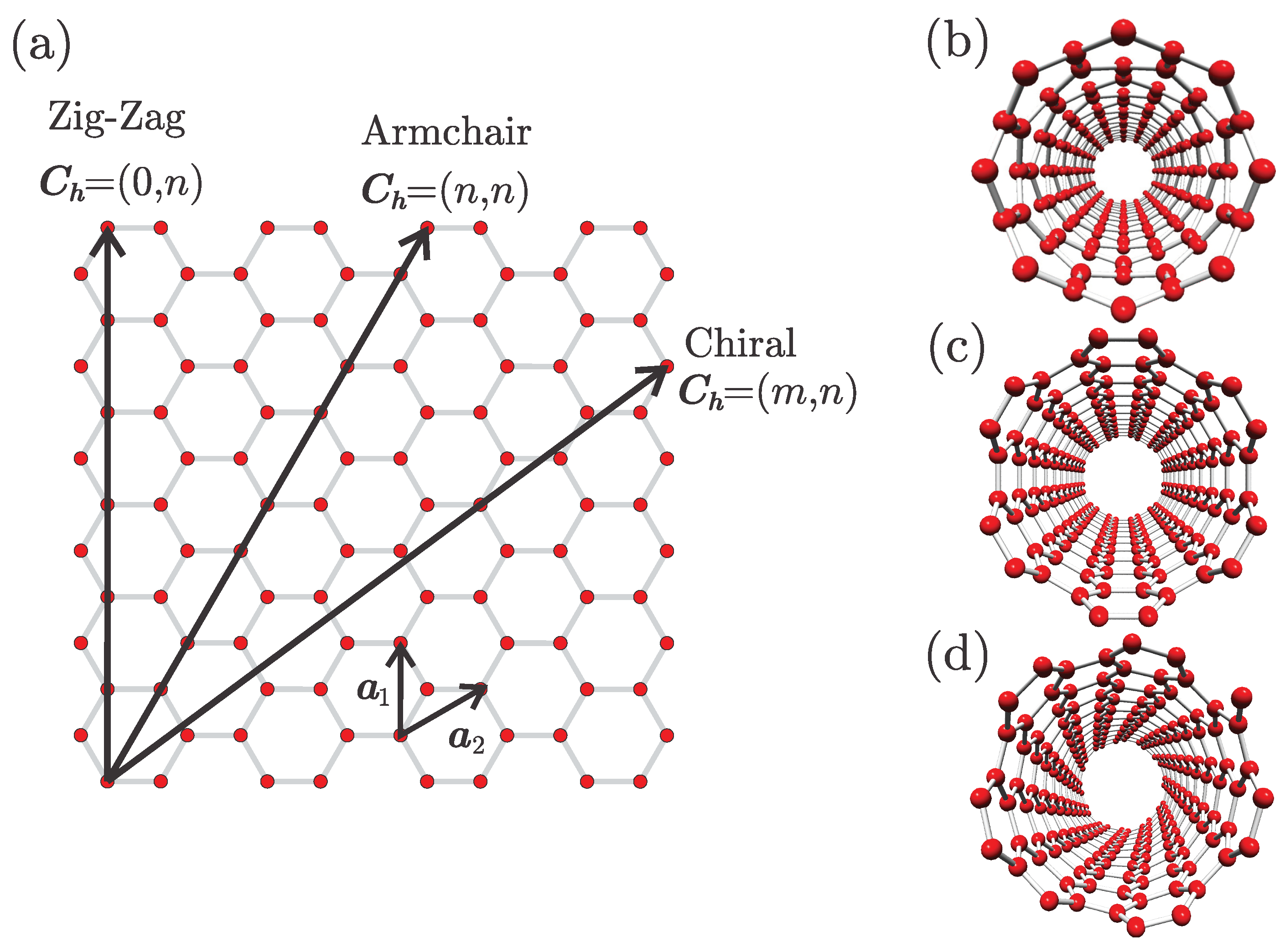
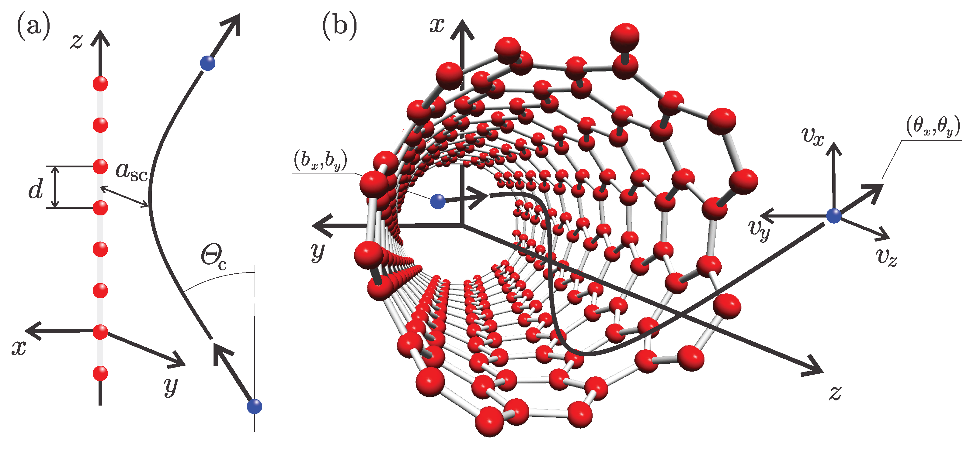
Here we consider the transmission of the parallel, monochromatic, 1-GeV proton beam through SWCNT (11, 9), which is perfectly aligned with nanotube axis. The radius of the SWCNT is $R=0.689$ nm, and the number of its atomic strings is $N=1204$. Standard deviation of the carbon thermal motion ${\sigma }_{th}$ can be estimated from the Debye theory, which for the room temperature (T = 300 K) gives ${\sigma }_{th}=0.005$ nm. Screening length of carbon atom is $a_{\mathrm{sc}}=0.026$ nm.

The motion of the protons in the longitudinal direction is relativistic while its motion in the transverse direction is classical. The equations of motion (11) still hold. The only differences are that m should be replaced by the protons relativistic mass $m_r$ ($m_r/m=2.066$), and the relationship between initial kinetic energy $E_k$ and longitudinal linear momentum $p_z$ is $p_z^2{c}^2=E_k^2+2m{c}^2{E}_k$, where c is the speed of light [9]. The relativistically corrected critical angle is ${\overline{\Theta }}_c=\sqrt{\frac{2m{c}^2+2E_k}{2m{c}^2+E_k}}{\Theta }_c=0.268$ mrad.

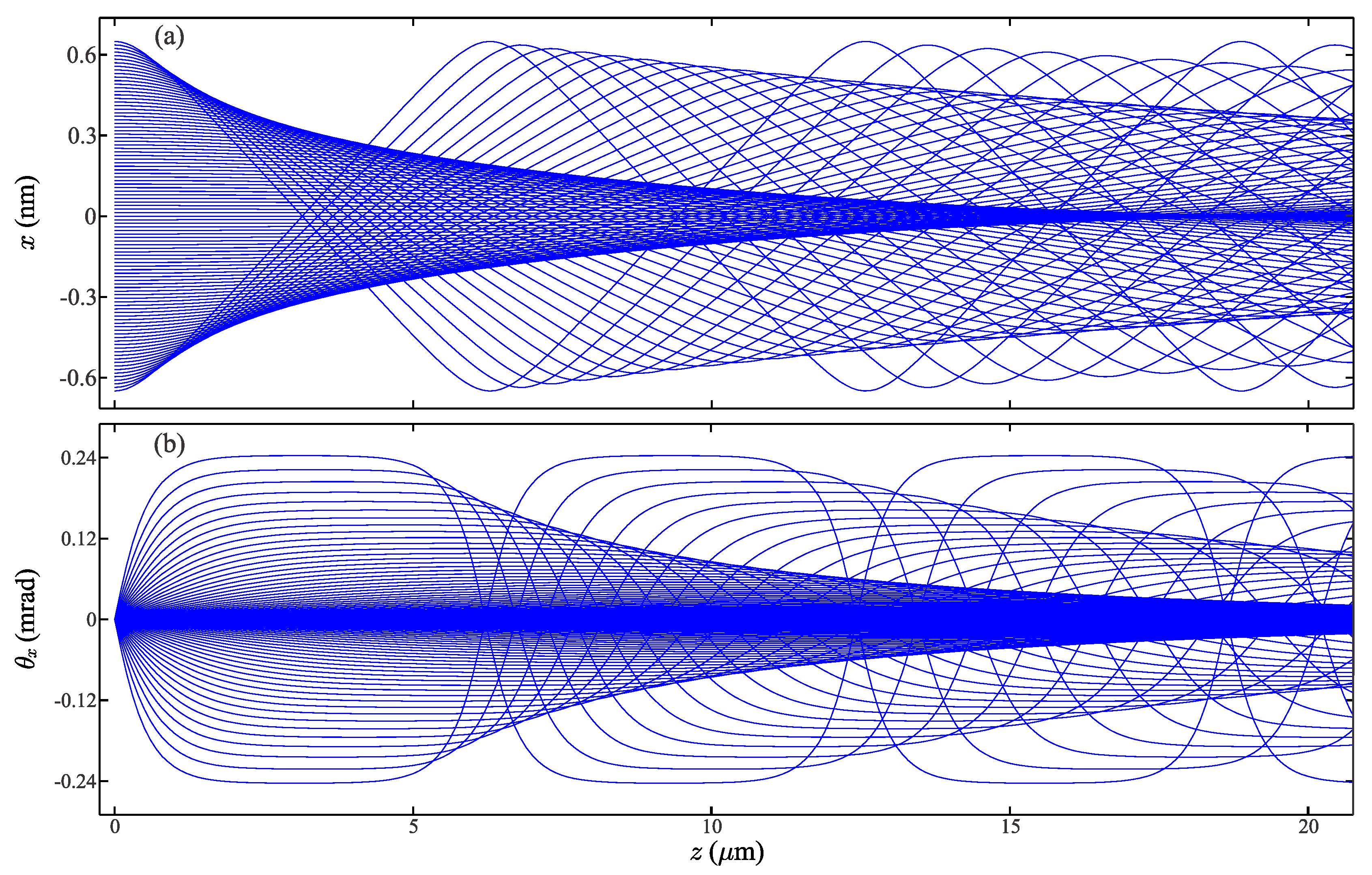
We consider only protons whose impact parameters satisfy inequality $|\mathit{b}|\le R-a_{\mathrm{sc}}$. Since the proton beam is aligned with the SWCNT axes, each proton trajectory is confined to a plane defined by the impact parameter $\mathit{b}$ and the nanotube axis. Figure 3 shows the obtained proton trajectories in the $x0z$ plane. Newton’s equations of motion (11) were solved by Runge-Kutta method of the 4-th order [41]. Note that the amplitude of any proton trajectory is constant and corresponds to its impact parameter $b_x$. The corresponding trajectories in the angular space are shown in Figure 3b. The amplitude of any trajectory is also constant. Note that the maximal deflection angle of ${\Theta }_c$ corresponds to the trajectory of impact parameter $b_x=R-a_{\mathrm{sc}}$. All these facts demonstrate that proton trajectories were accurately calculated.

Proton trajectories shown in Figure 3a,b can be concisely represented as function $x(z;b_x)$, ${\theta }_x(z;b_x)$, depending on the parameter $b_x$. For SWCNT of length L functions $x(L;b_x)$, ${\theta }_x(L;b_x)$ define mappings of the impact parameter plane to the final transmitted position and final transmitted angle plane, called the spatial and angular transmission function, respectively, which will be denoted as $X(b_x)$ and ${\Theta }_x(b_x)$. The symmetry of the trajectory family requires that both transmission functions are odd functions $X(b_x)=-X(-b_x)$, ${\Theta }_x(b_x)=-{\Theta }_x(-b_x)$. Rainbow defining condition (13) now reduces to

$$\frac{\mathrm{d}X(b_x)}{\mathrm{d}{b}_x}=0,\frac{\mathrm{d}{\Theta }_x(b_x)}{\mathrm{d}{b}_x}=0.$$

(23)

Therefore, the critical points of transmission functions, which occur in symmetrical pairs, are rainbow points. Each critical point pair corresponds to the one circular rainbow line whose radius is equal to the absolute value of the critical point ordinate.

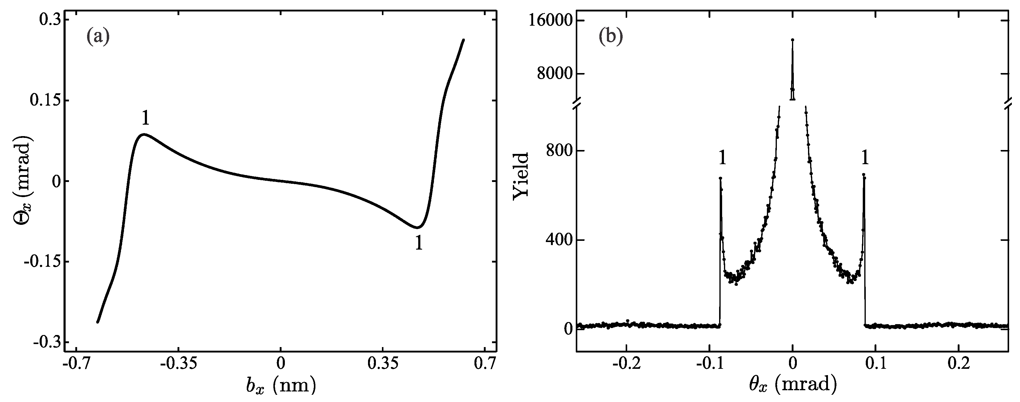
For the 10-$\mathsf{\mu }$m long SWCNT (11, 9) angular transmission function ${\Theta }_x(b)$, shown in Figure 4a, has only one critical point pair $(-b_x^{(1)},{\theta }_x^{(1)})$ = ($-0.493$ nm, 0.856 mrad), and $(b_x^{(1)},-{\theta }_x^{(1)})=(0.493$ nm, $-0.856$ mrad), both labeled 1. This function shows that for any ${\theta }_x$ from the interval $(-{\theta }_x^{(1)},{\theta }_x^{(1)})$ mrad, there are three corresponding impact parameters, while outside of this interval the correspondence is one-to-one. Therefore, there is only one circular angular rainbow line of radius 0.856 mrad. The interior of the line is the rainbow’s bright side, while its exterior is the rainbow’s dark side.

The vertical slice through the corresponding angular distribution is shown in Figure 4b. The initial number of protons was 16,655,140, while the size of the bin in the ${\theta }_x$ space was 0.866 μrad. Note the small statistical fluctuation of the obtained distribution which reflects the randomness of the impact parameter selection process. Besides this the obtained distribution is perfectly axially symmetric. This distribution contains three prominent peaks. The central peak is the consequence of the fact that potential $U_{{\mathit{C}}_{\mathit{h}}}^{th}$ has its minimum at the coordinate origin. It represents the undeflected part of the proton beam, and it is not related to the rainbow effect. The two remaining peaks are located symmetrically around the central maximum. Angular positions of the critical points form Figure 4a are indicated by the number 1. It is obvious that their positions are in the perfect correspondence with the positions of the mentioned peaks. Note also high particle yield inside, and low yield outside the interval enclosed by the observed peak pair, which corresponds to the rainbow light and dark sides. Therefore, the angular distribution contains one circular rainbow line whose properties are determined by the critical points of the transmission function.

3.2. Semi-Classical Interpretation of Quantum Rainbow Effect

This subsection is devoted to the analysis of the channeling of 1-MeV positrons through 200-nm long chiral SWCNT (14, 4). The radius of this nanotube is $R=0.650$ nm, while the number of atomic strings is $N=536$. Longitudinal motion of 1-MeV positrons is free and relativistic ($m_r/m=2.957$) while transverse motion is quantum and nonrelativistic. As in the previous example, Equation (16) still holds if bear mass m is replaced with relativistic mass $m_r$ [9]. To observe channeling effect one need to use positron beam collimated better then critical channeling angle ${\Theta }_c$. Here we assume that the incoming positron beam has angular standard deviation ${\Delta }_{\theta }=0.1{\Theta }_c$, which gives ${\sigma }_{\theta }=0.735$ mrad and ${\sigma }_{\rho }=0.134$ nm. This value was selected because then transverse size of any wave packet is large enough that the self-interference effect becomes significant, while on the other hand it is small enough to allow explicit dependence of their dynamics on impact parameters to be analyzed. Let M represent the number of wave packets uniformly covering impact parameter plane. Expansion coefficients from Equation (19) are $w_{\mathit{b}}=1/M$. In order that $Y_{\rho }(\mathit{\rho },0)$ be a uniform distribution in the entrance plane of the nanotube, the number of wave packets M must be very large (theoretically infinite). In order to minimize the number M an algorithm was devised which optimize the values of the coefficients $w_{\mathit{b}}$ while keeping the difference between the distribution $Y_{\theta }$ and uniform distribution $1/(\pi {(R-a_{\mathrm{sc}})}^2)$ in the region $\rho \le R-a_{\mathrm{sc}}$ below some prescribed tolerance. We have found that accurate representation of the initial distribution of the positron beam can be accomplished with only 142 Gaussian wave packets.

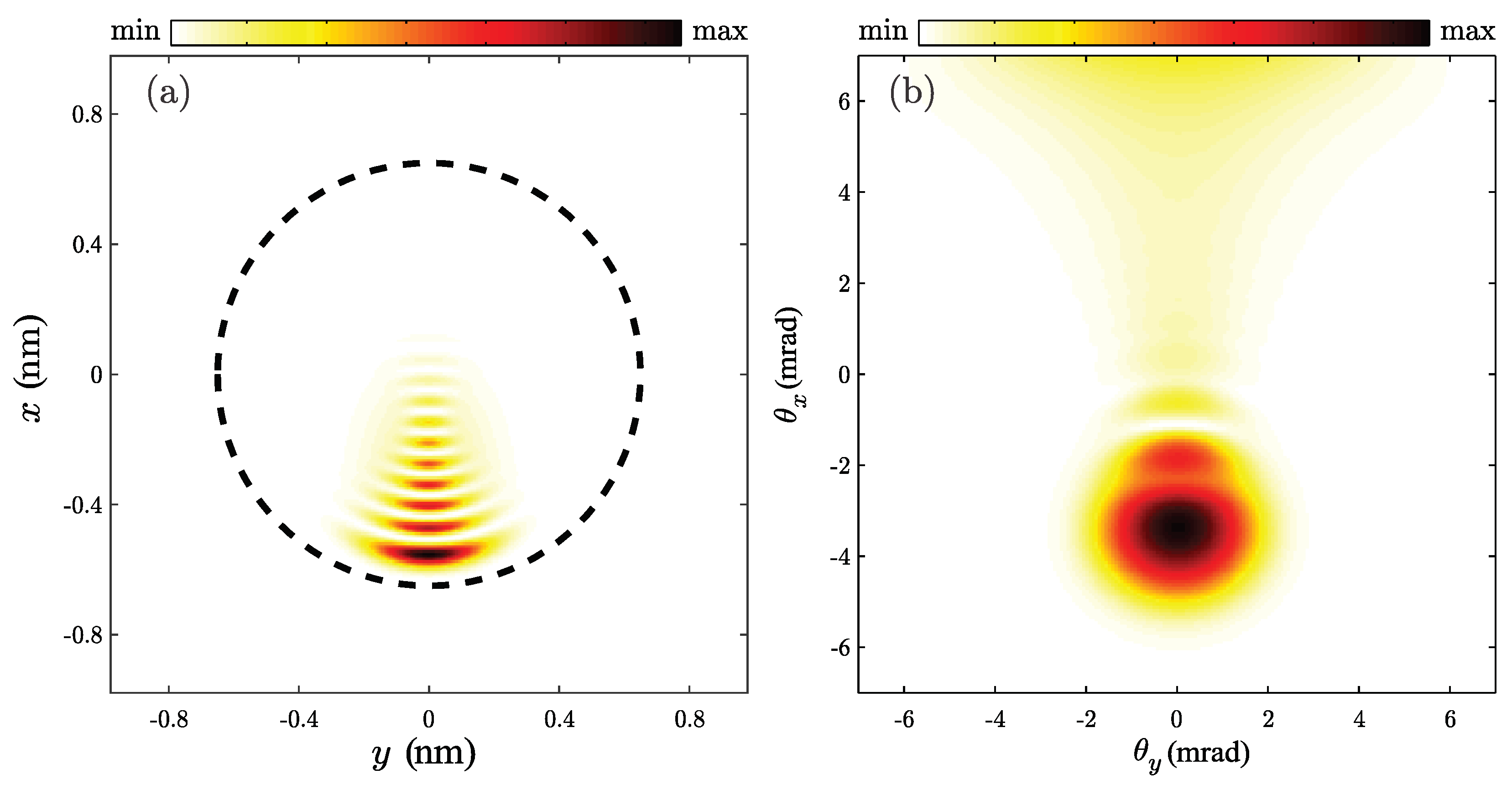
Let us examine the motion of the wave packet of impact parameter $\mathit{b}=(0.624,0)$ nm. The corresponding Schrödinger Equation (16) is solved using the method of Chebyshev global propagation [42]. The obtained probability densities at the exit of the SWCNT are shown in Figure 5. In both representations, densities have a number of peaks, which can be attributed to self-interference of the incoming part of wave function with the part of wave function already reflected from SWCNT wall. However, since all peaks are the consequence of the wave packet self-interference looking only on the numerically obtained probability densities, it is very difficult to say which peak is connected with the rainbow effect, and which one is a simple manifestation of the positron wave nature.

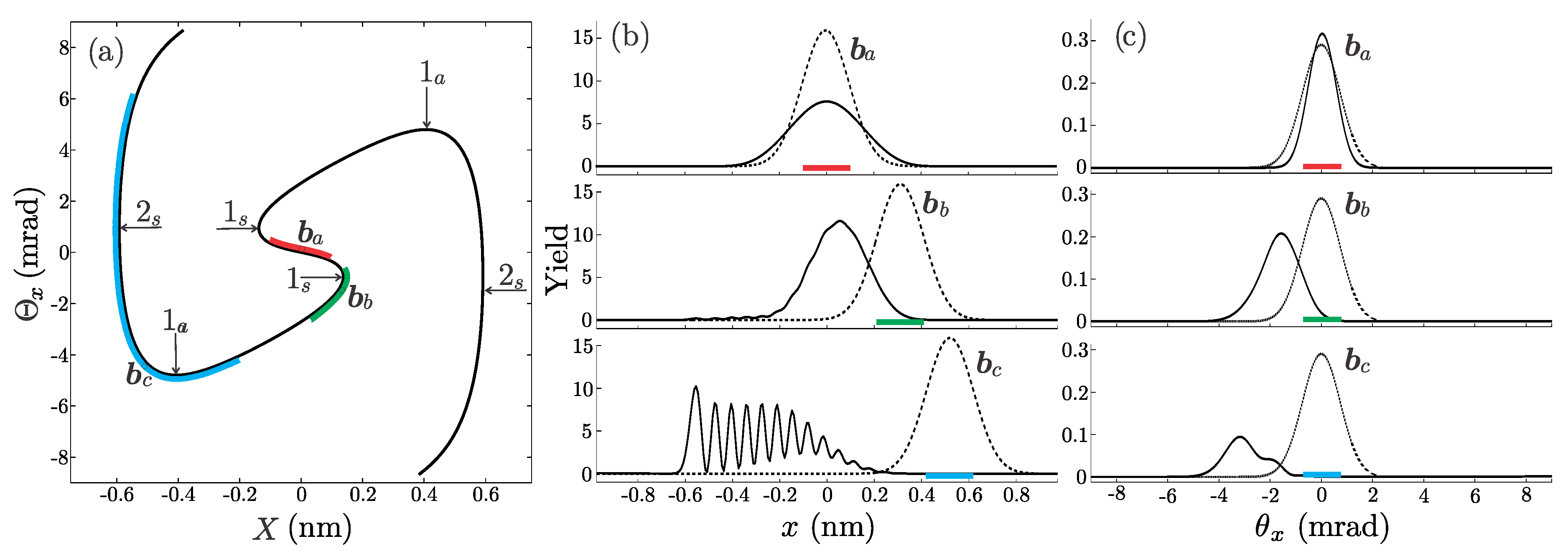
In order to understand and classify self-interference peaks, a semiclassical approach can be applied. To avoid unnecessary complications here we will focus only on the vertical slices of the wave packets moving along the x axis. Transmission functions $X(b_x)$ and ${\Theta }_x(b_x)$ then fully characterize the classical motion of the particle. In the phase space, those two functions define a curve called the rainbow diagram which is shown in Figure 6a as a thin black line. The transmission function $X(b_x)$ has two pairs of critical points labeled $1_s$ and $2_s$ whose ordinates are $\pm 0.14$ nm, and $\pm 0.59$ nm, respectively, while transmission function ${\Theta }_x(b_x)$ has only one pair of critical points labeled $1_a$ whose ordinates are $\pm 4.97$ mrad. The positions of the rainbow points in the rainbow diagram are indicated by the black arrows. Note that at rainbow points, the tangents of the rainbow diagram are vertical or horizontal. They represent points where different branches of the mappings ${\Theta }_x(X)$, and $X({\Theta }_x)$, respectively, meet. Therefore, mapping ${\Theta }_x(X)$ has 5 branches, while mapping $X({\Theta }_x)$ has only 3.

In the semiclassical approach the quantum wave function at the time t can be constructed from classical rainbow diagram as a sum of the contributions of the wave trains coming from all branches [43]. The contribution of the branch $\mu$ is of the form ${\rho }_{\mu }^{1/2}exp[i{S}_{\mu }/\hslash ]$. Let density of the trajectories in the impact parameter plane be $K(b)$. The number of particles in the interval $\mathrm{d}x$ around x coming from the branch $\mu$ is equal to the number of particles in the interval $\mathrm{d}{b}_x$ around the point $b_x$ mapped to the corresponding interval. Therefore, ${\rho }_{\mu }\mathrm{d}x=K_{\mu }(b_x)\mathrm{d}{b}_x$, where $K_{\mu }(b_x)$ is the density of the points in the branch $\mu$. The phase $S_{\mu }$ is a type 2 canonical transformation $\mathrm{d}{S}_{\mu }=\hslash k_z{\theta }_x\mathrm{d}x$ in the spatial representation and type 1 canonical transformation $\mathrm{d}{S}_{\mu }=\hslash k_{z}x\mathrm{d}{\theta }_x$ in the angular representation, of the branch $\mu$. Therefore, the total semiclassical wave functions in spatial and angular representations are given by the expressions

$$\begin{array}{ccc}\hfill {\psi }_{\mathrm{sc}}(x)& =& {\displaystyle \sum _{\mu }}\sqrt{K_{\mu }}{\left|\frac{\mathrm{d}{b}_x}{\mathrm{d}{X}_{\mu }}\right|}^{\frac{1}{2}}exp\left[i{k}_z{\int }_{X_{\mu }^{(0)}}^x{\Theta }_x^{\mu }(X^{\prime })\mathrm{d}{X}^{\prime }\right],\hfill \\ \hfill {\phi }_{\mathrm{sc}}({\theta }_x)& =& {\displaystyle \sum _{\nu }}\sqrt{K_{\nu }}{\left|\frac{\mathrm{d}{b}_x}{\mathrm{d}{\Theta }_x^{\nu }}\right|}^{\frac{1}{2}}exp\left[i{k}_z{\int }_{{\Theta }_{\nu }^{(0)}}^{{\theta }_x}{X}_{\nu }({\Theta }_x^{\prime })\mathrm{d}{\Theta }_x^{\prime }\right],\hfill \end{array}$$

(24)

where indices $\mu$, and $\nu$ count branches of the spatial and angular transmission functions $X_{\mu }({\Theta }_x)$, and ${\Theta }_x^{\nu }(X)$, respectively, $X_{\mu }^{(0)}$, and ${\Theta }_{\nu }^{(0)}$ are referent points of the $\mu$-th and $\nu$-th branch respectively. Note that ${\Theta }_x^{\mu }(X)$ stands for the inverse function of the branch $X_{\mu }({\Theta }_x)$ of spatial transmission function, while $X_{\nu }({\Theta }_x)$ is inverse function of the branch ${\Theta }_x^{\nu }(X)$ of the angular transmission function. In the spatial representation the sum should be taken over all branches satisfying equation $X_{\mu }=x$, while in the angular representation the sum is over all branches satisfying equation ${\Theta }_x^{\nu }={\theta }_x$.

Let us now apply semiclassical reasoning for interpretation of the quantum motion of wave packets labeled a, b and c of impact parameters ${\mathit{b}}_{\mathit{a}}$ = (0, 0), ${\mathit{b}}_{\mathit{b}}$ = (0.31, 0), and ${\mathit{b}}_{\mathit{c}}$ = (0.52, 0) nm, respectively. Their spatial, and angular representations are shown in Figure 6b,c respectively. Wave packets in the impact parameter plane are shown by the dashed lines, wave packets in the exit plane of the SWCNT are shown by the solid line. Since the initial distributions are Gaussian, the dominant contribution comes from trajectories from the interval $[b_x-{\sigma }_{\rho },b_x+{\sigma }_{\rho }]$. For reasons of simplicity, the contributions of all other trajectories will be neglected. The dominant intervals are in Figure 6b shown by the red, green, and blue lines, respectively. In the angular space, the dominant intervals of length of $2{\sigma }_{\theta }$ are in Figure 6c designated by the same colors. The corresponding exit positions of the trajectories from the dominant intervals are in Figure 6a indicated by thick red, green and blue lines, respectively. For wave packer a, the red curve in Figure 6a covers only one branch of the mappings $X({\Theta }_x)$ and ${\Theta }_x(X)$, respectively. This is the reason why for wave packet a self-interference is not observable. For wave packet b the green line in Figure 6a covers one branch of mapping $X({\Theta }_x)$ completely and slightly extends into the second branch, and covers only one branch of the mapping ${\Theta }_x(X)$. Therefore, the number of trajectories which interfere is small. This explains why in the spatial representation for wave packet b only weak self-interference can be observed, and there is no observable self-interference in the angular representation. For wave packet c the blue curve in Figure 6a covers two branches of mappings $X({\Theta }_x)$ and ${\Theta }_x(X)$, respectively. In this case, the number of trajectories which interfere is large. This fact explains why self-interference is the strongest for wave packet c.

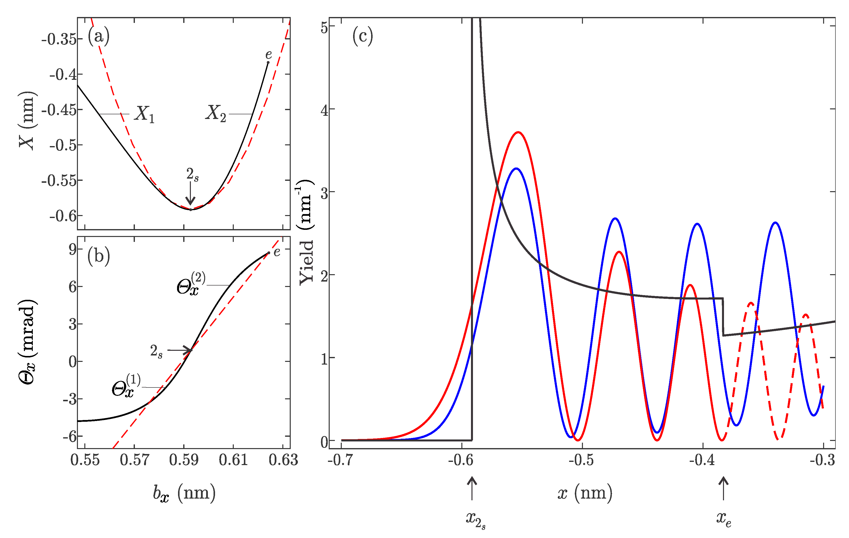
Let us now examine more closely shape of the classical, the semi-classical probability density of the wave packet c in the vicinity of the point $2_s$, and compare it with the exact solution given on Figure 6b. The spatial transmission function $X(b_x)$ is shown in Figure 7a has a minimum labeled $2_s$ at the point at $(b_{2_s},x_{2_s})$. It ends at the point e which correspond to maximal possible considered impact parameter $b_e=R-a_{sc}$. The inverse transmission mapping $b_x(x)$ have two branches labeled $X_1$ and $X_2$, respectively. The branch $X_1$ is formed by the end positions of positrons having impact parameters $b_x<b_{2_s}$, while positrons ending on the branch $X_2$ have impact parameters belong to the interval $[b_{2_s},b_e]$. Therefore, for $x<x_{2_s}$ the mapping $b_x(x)$ is zero-valued for x in the interval $[x_{2_s},x_e]$, the mapping is double-valued, while for $x>x_e$ it is single-valued. The classical probability density is defined by the equation

$$\rho (x)={\left\{K_1(b_x(X_1))\left|\frac{\mathrm{d}{b}_x}{\mathrm{d}{X}_1}\right|\right\}}_{X_1=x}+{\left\{K_2(b_x(X_2))\left|\frac{\mathrm{d}{b}_x}{\mathrm{d}{X}_2}\right|\right\}}_{X_2=x}.$$

(25)

For an interval of impact parameters that is considered to be small from Figure 7a, function $K(b_x)$ can be approximated with a constant (this also means that $K_1(b_x)=K_2(b_x)=K$). The resulting normed distribution $\rho (x)$ is in Figure 7c shown by the black line. Since, $\frac{\mathrm{d}{X}_1}{\mathrm{d}{b}_x}=\frac{\mathrm{d}{X}_2}{\mathrm{d}{b}_x}=0$ for $b_x=b_{2_s}$ both branches give singular contributions to the function $\rho$ which is infinite at the rainbow point $x_{2_s}$. For $x<x_{2_s}$ density $\rho (x)=0$, therefore this region is the dark side of the rainbow. For x in the interval $[x_{2_s},x_e]$ the function $\rho (x)$ is monotonously decreasing. Note an abrupt jump of the function $\rho (x)$ at $x=x_e^{+}$ which is consequence of the change of the multiplicity of the mapping $b_x(x)$ from 2 to 1.

The exact normed probability density $|{\psi }_c{(x)|}^2$ is shown in the Figure 7c by the blue line. Comparison of these two solutions shows the following. The classical approximation correctly predicts overall order of the magnitude of the exact probability density $|{\psi }_c{(x)|}^2$. It predicts that the largest contribution to the density is at the rainbow point $x_{2_s}$, which is very close to the largest peak of the function $|{\psi }_c{(x)|}^2$, and that density is low for $x<x_{2_s}$ and high for $x\ge x_{2_s}$. Out of many peaks of the density $|{\psi }_c{(x)|}^2$, as is clearly visible on Figure 6b and Figure 7c, the classical approximation explains the existence of only one, and clearly overestimates its amplitude.

According to the Equation (24) to construct semiclassical solution ${\psi }_{sc}(x)$ one need to find all solution of the equation $X=x$, form semiclassical waves and sum their contributions. For example, if $x\in [x_{2_s},x_e]$ amplitudes of the individual semiclassical waves are ${(K\frac{\mathrm{d}{b}_x}{\mathrm{d}{X}_1})}^{1/2}$ and ${(K\frac{\mathrm{d}{b}_x}{\mathrm{d}{X}_2})}^{1/2}$. To obtain phases of the semiclassical waves one need to consider also angular transmission function ${\Theta }_x(b_x)$ shown in Figure 7b. Since the mapping $b_x(X)$ is two-valued in the considered interval, the mapping ${\Theta }_x(b_x(X))$ has also two branches ${\Theta }_x^{(1)}(b_x(X_1))$, and ${\Theta }_x^{(2)}(b_x(X_2))$. Phases of the semiclassical waves are solutions of the equations $\frac{\mathrm{d}{S}_1}{\mathrm{d}{X}_1}=k_z{\Theta }_x^{(1)}(X_1)$, and $\frac{\mathrm{d}{S}_2}{\mathrm{d}{X}_2}=k_z{\Theta }_x^{(2)}(X_2)$.

Note that direct evaluation of the Equation (24) is not possible at $x=x_{2_s}$ since both wave amplitudes ${(K\frac{\mathrm{d}{b}_x}{\mathrm{d}X})}^{1/2}$ diverge. To circumvent this limitation one can use the so-called transitional approximation [11,29]. Firstly, the spatial and the angular transmission functions are in the vicinity of the rainbow point $2_s$ approximated by the following polynomials

$$X(b_x)={\alpha }_2{b}^2+{\alpha }_{1}b+{\alpha }_0,{\Theta }_x(b_x)={\beta }_{1}b+{\beta }_0.$$

(26)

Obtained approximations are in Figure 7a,b shown by the dashed red lines. By the analytical continuation validity of the equation $X=x$ is extended to the whole complex plane. Therefore, for $x\in [x_{2_s},x_e]$ equation $X=x$ has two real solutions, for $x=x_{2_s}$, the equation has a double root, while for $x<x_{2_s}$ the equation has two conjugate complex solutions. Taking into account additional complex solutions it can be shown that transitional semiclassical density $|{\psi }_{sc}^{(t)}{(x)|}^2$ is given by the equation

$$|{\psi }_{sc}^{(t)}{(x)|}^2=\frac{{\beta }_1^{1/3}{k}_z^{1/3}K}{2\pi {\alpha }_2^{2/3}}{\left|\mathrm{Ai}\left(\frac{{\beta }_1^{1/3}{k}_z^{1/3}}{{\alpha }_2^{1/3}}(x-x_{2_s})\right)\right|}^2,$$

(27)

where $\mathrm{Ai}$ is the Airy function [37]. The obtained semiclassical distribution $|{\psi }_{sc}^{(t)}{|}^2$ is in Figure 7c shown by the red line. The largest maxima which is now finite of the function $|{\psi }_{sc}^{(t)}{|}^2$ is the closest to the classical rainbow $2_s$. For $x<x_{2_s}$ interference of the complex rays make density $|{\psi }_{sc}^{(t)}{|}^2$ exponentially decaying. For $x\ge x_{2_s}$ a number of smaller peaks can be observed which appear due to the constructive interference of the real rays.

Note that almost identical expression describe semiclassical intensity of the light in the vicinity of the optical rainbow [44,45,46]. Therefore, peaks of the function $|{\psi }_{sc}^{(t)}{|}^2$ can be classified in analogues way as interference peaks of the optical rainbow. The large maximum closest to the position of the classical rainbow is considered to be the primary rainbow maximum, while all other peaks are supernumeraries associated with the observed primary.

Comparison of the red and the blue curve from Figure 7c reveals that transitional semiclassical approximation almost perfectly predicts the position and size of the dominant peak of the exact distribution $|{\psi }_c{|}^2$. The constructive interference of real rays explains the existence of all other maxima, while the interference of the complex rays explains how probability density $|{\psi }_c{|}^2$ can have non-zero values in the region where there are no real rays at all. It could be said that the ray interference “assuages” the sharpness of the classical distribution $\rho (x)$. Therefore, the semiclassical approximation captures all qualitative features of the quantum rainbow scattering effect. However, its validity is limited. Note that accuracy of the semiclassical solution $|{\psi }_{sc}^{(t)}{|}^2$ actually decreases for $x>x_{2_s}$. Its range of validity is limited only to the region $x\le x_e$. The reason for this is that in the vicinity of the point $x=x_e$ the multiplicity of the inverse transmission function $b_x(X)$ changes by one, while number of real roots of any polynomial approximation of the $X(b_x)$ can change only by an integer multiple of 2. This is the reason why semiclassical density $|{\psi }_{sc}^{(t)}{|}^2$ for $x>x_e$ in Figure 7c is shown by the dashed red line. For $x>x_e$ the correct semiclassical wave function is given by only one semiclassical wave. According to the Equation (24) semiclassical density is then $|{\psi }_{sc}{(x)|}^2=K\frac{\mathrm{d}{b}_x}{\mathrm{d}{X}_1}$, i.e., it is equal to the classical solution $\rho (x)$. Therefore, the semiclassical approximation is not capable of explaining the existence of the peaks of the exact density $|{\psi }_c{|}^2$ in the region where transmission function has only one branch.

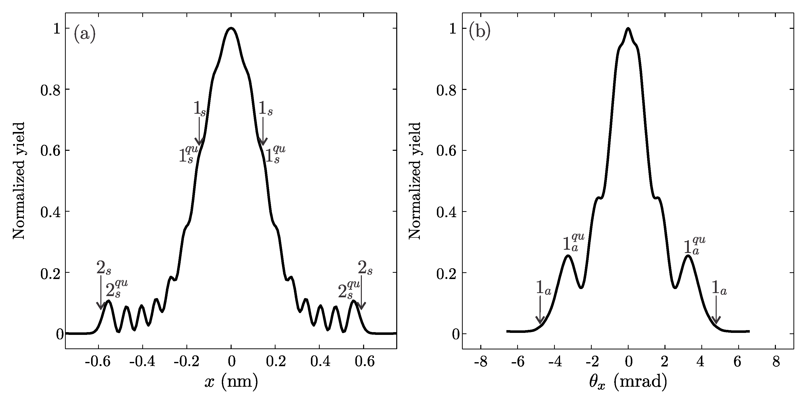
Summing contributions of all wave packets according to Equation (19) gives distributions of the transmitted positron beam at the exit plane of the SWCNT. The vertical slices through the obtained distributions in spatial and angular space are shown in Figure 8a,b, respectively. Each pair of symmetric maxima visible in the Figure 8a,b corresponds to the circular maxima of the 2D distribution. Positions of the classical rainbow point pairs $1_s$, $2_s$, and $1_a$ are indicated by the arrows. Large maxima closest to the classical rainbow points, labeled $1_s^{qu}$, and $2_s^{qu}$ in the Figure 8a at $x_{1s}^{qu}=\pm 0.55$ nm and $x_{2s}^{qu}=\pm 0.14$ nm are interpreted as the primary and the secondary rainbow point. All other peaks are considered to be supernumerary rainbows. In the case of angular distribution, the large maximum pair $1_a^{qu}$ at ${\theta }_{1a}^{qu}=\pm 3.27$ mrad, closest to the classical rainbow peaks $1_a$, are interpreted as the primary rainbow points, all remaining peaks are considered to be supernumerary rainbows.

3.3. Morphological Interpretation of Quantum Rainbow Effect

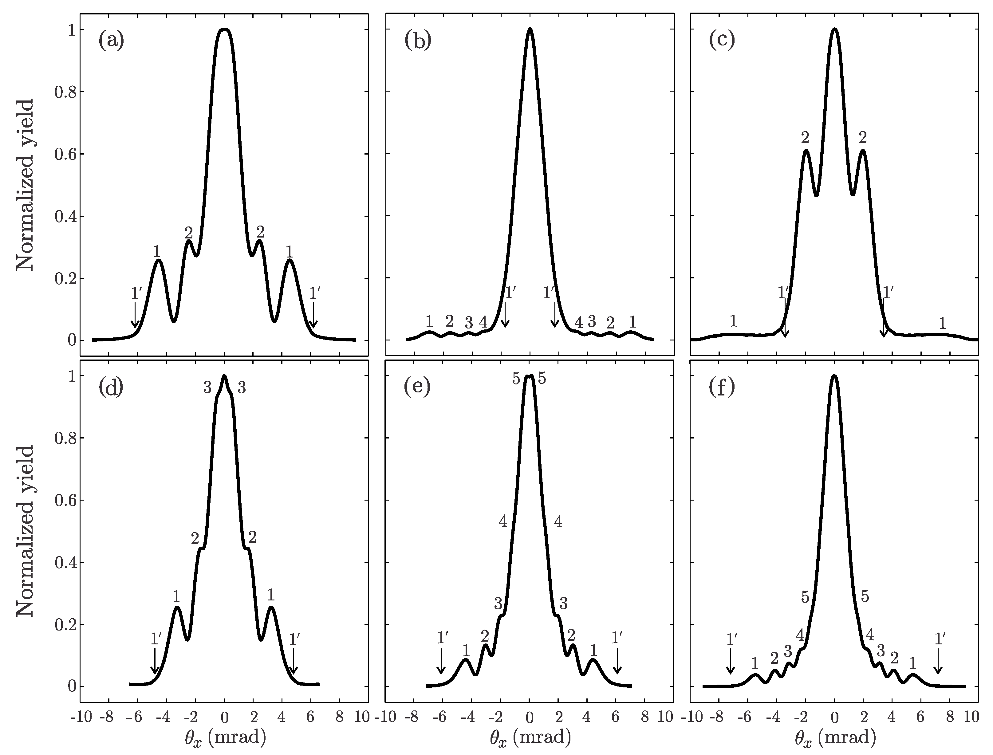
The developed method was applied for classification of angular distributions of 1-MeV positrons transmitted through 200-nm long SWCNTs (7, 3), (8, 5), (9, 7), (14, 4), (16, 5), and (17, 7). The nanotubes considered here are the easiest to produce by the arch discharge method [1]. The radii of the considered nanotubes are in the range from 0.35 to 0.85 nm. The classical critical angles for the considered SWCNTs are very close to each other, ranging from 7.3 to 7.4 mrad. For all SWCNT we assume that initial angular standard deviation of the positron beam ${\Delta }_{\theta }$ is always equal to the 10% of the corresponding classical critical angle ${\Theta }_c$. This means that the used angular standard deviations of the positron beams are in the range [0.73, 0.74] mrad, the corresponding range of the standard deviations of the Gaussian wave packets are in range [0.094, 0.095] nm. Note that all wave packets have almost the same size.

Vertical slices through obtained distributions are shown in Figure 9. Initial spatial distributions were constructed using: 43, 71, 101, 141, 190, 241 Gaussians, respectively. All prominent peaks excluding central are labeled by numbers, with symmetrical maxima labeled by the same number. Numeration always starts from the outermost rainbow pair. In all analyzed cases there is only one classical rainbow point pair labeled $1^{\prime }$. Their positions in Figure 9 are shown by the arrows. It is clear that the quantum peak pairs labeled 1 in Figure 9a,d–f are quantum primary rainbow points. All other peaks are supernumerary rainbow.

It should be noted that the semiclassical classification of the quantum peaks for the distributions from Figure 9b,c is ambiguous. This is not surprising since the applicability of the semiclassical approach is limited. Rather, it is surprising that the semiclassical interpretation works at all. It should be noted that accurate wave functions differ considerably from their semiclassical counterparts. If we take a closer look at the wave packet ${\mathit{b}}_{\mathit{c}}$ shown in Figure 6b,c, the interference is clearly visible in the interval from $-0.6$ nm up to $0.2$ nm in the spatial representation, and in interval from $-5$ mrad up to the $-1$ mrad. However, the corresponding relevant parts of the transmission functions are two-valued only in the intervals $[-0.6,-0.5]$ nm, and $[-6,-4]$ mrad, respectively. Outside the mentioned intervals the transmission functions are single-valued, and there should be no observable interference effects. Therefore, the semiclassical wave functions drastically underestimate real self-interference of the wave packets.

The problem with the semiclassical interpretation is that it intrinsically relay on classical concepts (such as exact position of the particle in the phase space) which do not have direct quantum analogue. A alternative approach would be to try to link the rainbow effect to certain morphological properties of the family of the classical trajectories, and quantum amplitude and phase function families. If morphological properties were found to be equal then both approaches are merely two descriptions of the same physical reality.

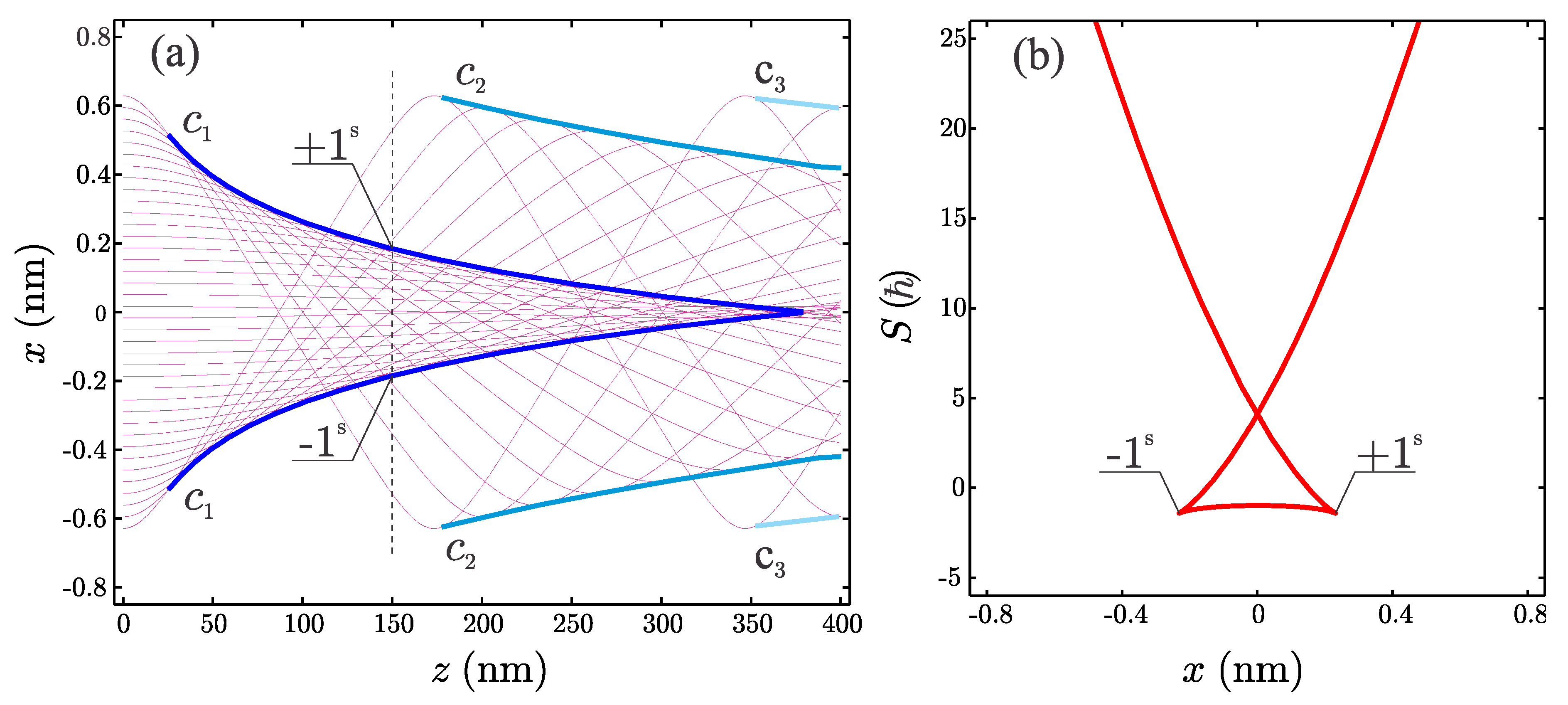
In this subsection it will be shown that it is possible unambiguously to classify quantum peaks relaying only on the information contained in the quantum amplitude and phase function families. In order to show that let us examine channeling of 1-MeV positrons through 400-nm long SWCNT (11, 9). The classical critical angle is ${\Theta }_c=7.3$ mrad. The obtained trajectory family in $xOz$ plane is shown in Figure 10a. The striking features of this family are three pairs of envelope lines, labeled $c_1$, $c_2$, and $c_3$, which are defined as a limiting line formed from intersections points of the neighboring family members [47]. The mathematical envelope is defined as a set of solutions of the equation

$$\frac{\partial }{\partial b_x}x(z;b_x)=0.$$

(28)

Equation (28) shows that each envelope is a locus of one critical point of the transmission function, i.e., the envelope is caustic line of the trajectory family [48]. For example, for a nanotube of length $L=150$ nm the spatial transmission function has one symmetrical pair of critical points whose ordinates $x_1^s=\pm 0.23$ nm are equal to the positions of envelope points $\pm 1^s$ in Figure 10a. Another important quantity is the Hamilton’s principal function defined by the equation [49]

$$\frac{\partial }{\partial x}S(x)=\hslash k_z{\theta }_x,$$

(29)

which is directly related to the phase function of the quantum wave packet [50]. Hamilton’s principal functions for nanotube whose length is $L=150$ nm is shown in Figure 10b. It is multivalued singular curve composed of three branches. The caustic lines are also loci of singularities of the Hamilton’s principal function [48]. Its cusped-like singular points, locally isomorphic to the cusp catastrophe [51], are also labeled $\pm 1^s$. Therefore, envelope lines and singularities of the Hamilton’s principal function are inextricably linked to the manifestations of the rainbow effect.

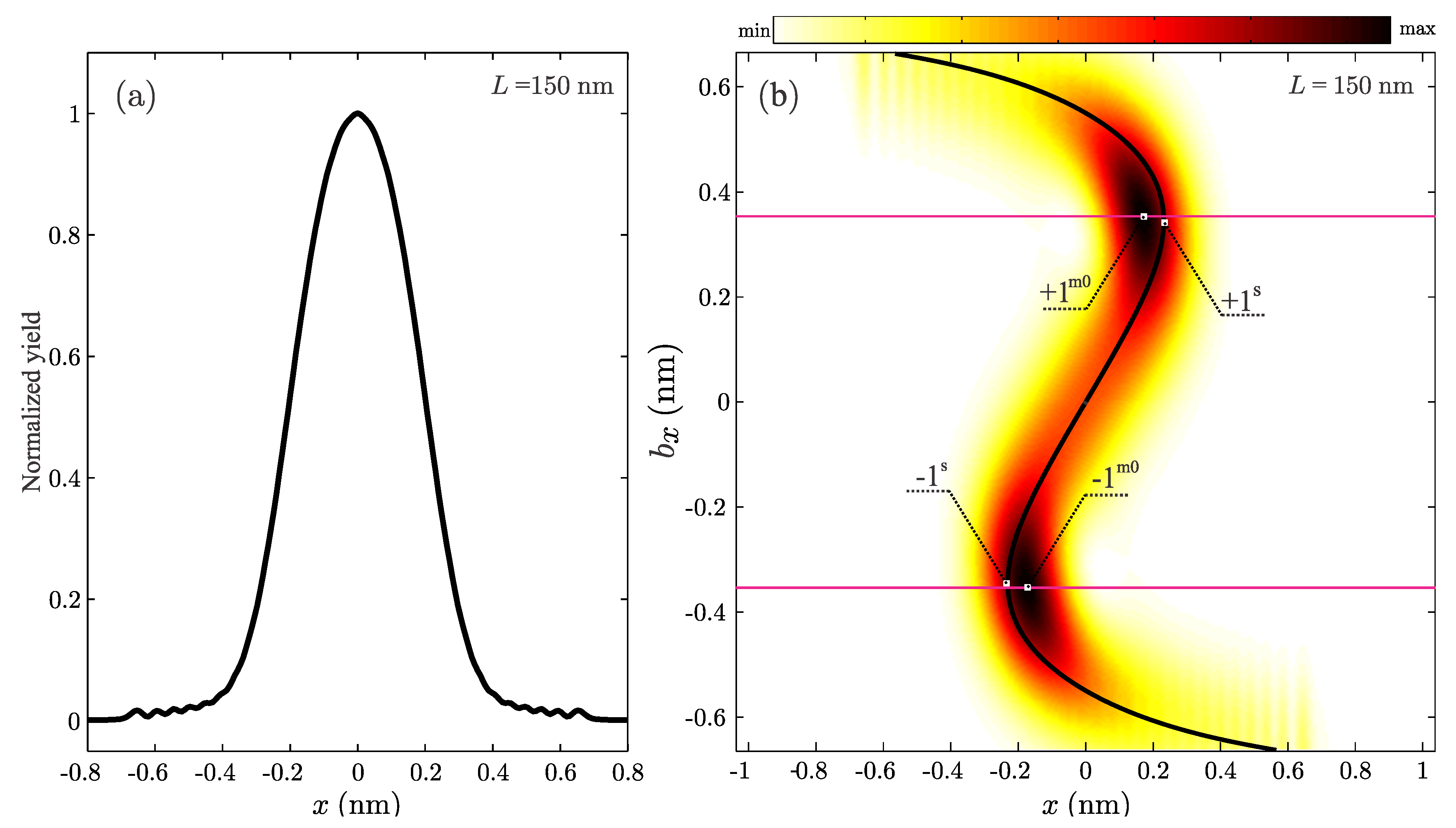
Now let us apply the same logic for the explanation of the quantum rainbow channeling. Figure 11a shows spatial distribution of the transmitted positron obtained assuming that initially its divergence was ${\Delta }_{\theta }=0.1{\Theta }_c$. Spatial and angular standard deviations of the wave packets were ${\sigma }_{\rho }=0.19$ nm and ${\sigma }_{\theta }=$0.73 mrad. The vertical slice through the obtained spatial distribution of the positron beam, transmitted through 150-nm long SWCNT (11, 9), is shown in Figure 11a. It consists of a large central peak which shows no signs of any internal structure, and six pairs of smaller peaks. The largest is the outermost peak pair, while remaining peaks are of approximately the same size. We need to provide a classification of the observed behaviour, and an explanation for its formation.

Since the obtained spatial distribution is axially symmetric we have focused only on the motion of wave packets with impact parameters belong to the nanotube vertical cross-section. We have followed evolution of 301 wave packets. Vertical cross-sections through obtained probability densities parameterized by the impact parameter are shown in Figure 11b. This distribution is dominated by two large maxima labeled $\pm 1^{m0}$ at $x^{m0}=\pm 0.17$ nm. Therefore, the dominant contribution to the large central peak in the Figure 11a actually comes from two smaller maxima. During their evolution, the wave packets become wrinkled (for example see Figure 5, or Figure 6b,c). This is the manifestation of the wave packet self-interference caused by the interaction with the nanotube walls. The wave packet ensemble shown in Figure 11b can be separated in two parts. The first one is formed by the wave packets showing no observable wrinkling (i.e., for $|b_x|<0.33$ nm). The second subensemble is formed by the wave packets for which self-interference is considerable (i.e., for $|b_x|\ge 0.33$ nm), which is called the rainbow subensemble. Members of these two subensembles are separated by the magenta lines in Figure 11b. Note the formation of the vertical yellow stripes which occur for the wave packets of impact parameters approximately in the range $|b_x|\ge 0.50$ nm. This means that the wave packets wrinkle in the mutually coordinated way. The corresponding inverse classical spatial transmission function is shown by the thick black line. Positions of the classical rainbow points, labeled $\pm 1^s$, are also indicated. Quantum probability density is concentrated around the classical line. It behaves as if there is a virtual barrier preventing spreading of the wave packets in the areas beyond the line.

It should be noted that the observed behavior is unexplainable by the semiclassical approach. For example, for $b_x>0.33$ nm the wave packet wrinkling is the most noticeable in rainbow subensemble and in the region $x<0.4$ nm, where the inverse transmission function is single valued. On the other hand the semiclassical approximation predicts that the most intense self-interference should be in the regions close to the classical rainbow points $\pm 1^s$, where no wave packet wrinkling can be observed.

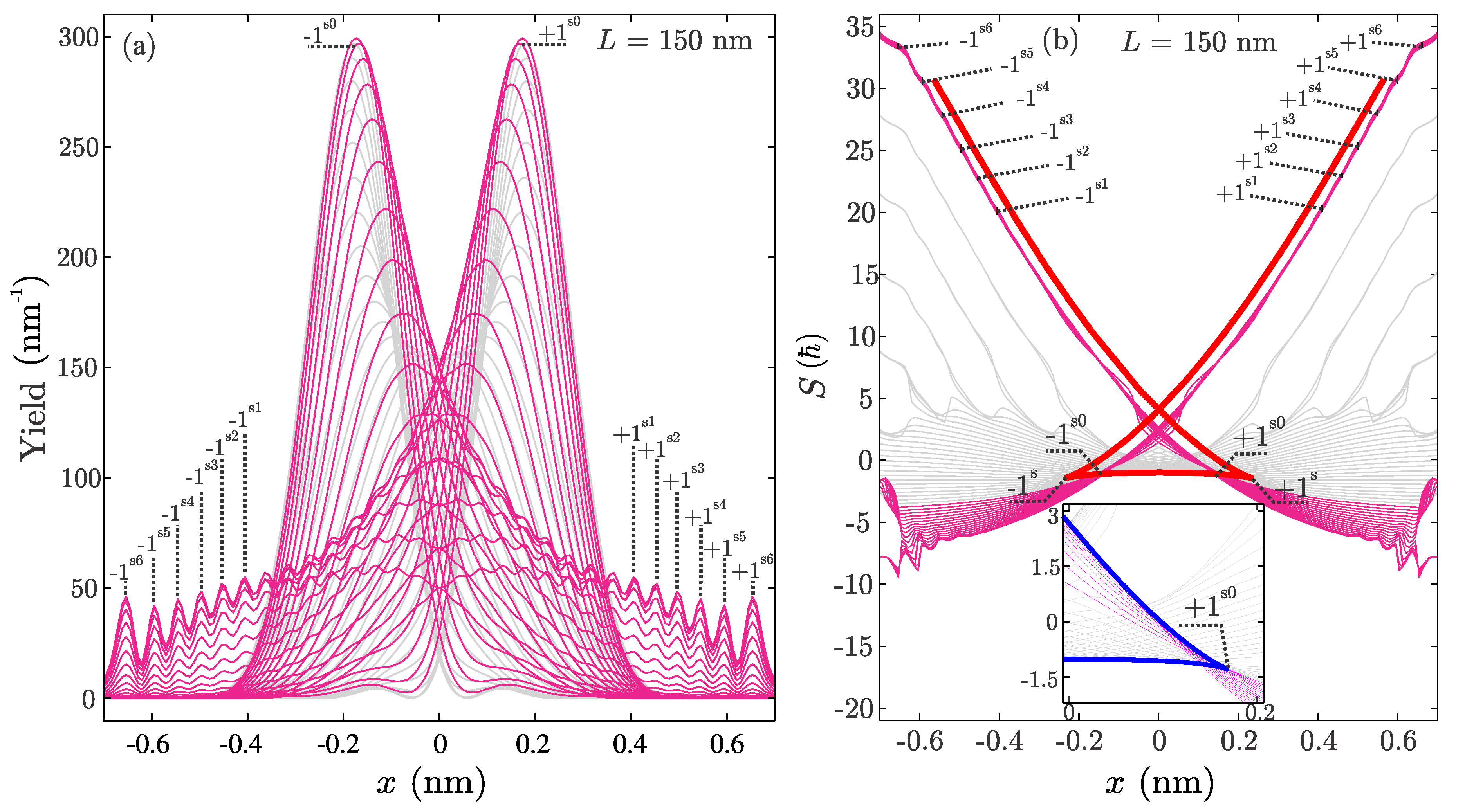
Wrinkling, concentration and coordination of the wave packets are elementary processes clearly sufficient for description of the wave packet motion. Out of these three processes, the coordination is the most important for explanation of the rainbow effect. Next, we will show that coordinated evolution of wave packets generate the rainbow effect. Figure 12a shows the family of quantum probability densities. Members of the rainbow subensemble are designated by the magenta lines. Each member represents the motion of the wave packet reflected form the SWCNT boundary. The largest maxima of any member show the current position of the wave packet center, with a large number of self-interference maxima on its tail. The remaining probability densities are shown by the gray lines. Prominent peak pairs visible in Figure 11a and Figure 12a labeled $\pm 1^{s0}$, $\pm 1^{s1}$, $\pm 1^{s2}$, $\pm 1^{s3}$, $\pm 1^{s4}$, $\pm 1^{s5}$, and $\pm 1^{s6}$, are at $x_1^{s1}=\pm 0.41$, $x_1^{s2}=\pm 0.45$, $x_1^{s3}=\pm 0.50$, $x_1^{s4}=\pm 0.55$, $x_1^{s5}=\pm 0.60$, and $x_1^{s6}=\pm 0.66$ nm, respectively. The numbering starts from the innermost peak pairs. The reason for such a convention will become apparent shortly. Note that due to the wave packet coordination, members of the rainbow subensemble have their respective maxima on the exactly same abscissas.

Figure 12b shows the obtained family of quantum phase functions expressed in the units of ℏ. The red line shows the corresponding classical Hamilton’s principal function form Figure 10b. Phases of the members of the rainbow subensemble are designated by the magenta lines, remaining phases are shown by the gray lines. The family of phase functions can also be subdivided into subsets of lines which run in parallel, i.e., subsets of coordinated wave packets. Note that the subset of magenta lines is the largest, which also runs in parallel with the classical Hamilton’s principal function. Therefore, wave packet coordination is the strongest in the rainbow subensemble. Detailed analysis of phases functions in the vicinity of classical singular points $\pm 1^s$ have shown that envelope function of phase function family also have two cusp singular points $\pm 1^{s0}$ at $x_1^{s0}=\pm 0.16$ nm. This can be seen in inset in Figure 12b where the envelope line is shown by the blue line. The "vertical" branch of the envelope is defined by the members of the rainbow subensemble, while the "horizontal" is defined by the remaining phases of the ensemble. Therefore, both subensembles are important for the explanation of the formation of cusp singular points. The position of the points $\pm 1^{s0}$ is also shown in Figure 12a and it proved to be very close to the peaks $\pm 1^{m0}$ from Figure 11b. A careful examination revealed that phases of the rainbow subensemble have common inflection points labeled $\pm 1^{s0}$, $\pm 1^{s1}$, $\pm 1^{s2}$, $\pm 1^{s3}$, $\pm 1^{s4}$, $\pm 1^{s5}$, and $\pm 1^{s6}$, respectively whose abscissas are equal with abscissas of the corresponding points in Figure 12a. Note that points $+1^{s1}$, $+1^{s2}$, $+1^{s3}$, $+1^{s4}$, $+1^{s5}$, and $+1^{s6}$, respectively belong to the branch generated by the point $-1^{s0}$.

Now the classification of the prominent peaks of the spatial distribution of the positron beam is straightforward. The central maximum consists of two primary quantum rainbow peaks $\pm 1^{s0}$. Peaks $+1^{s1}$, $+1^{s2}$, $+1^{s3}$, $+1^{s4}$, $+1^{s5}$, and $+1^{s6}$, respectively, are supernumeraries of the primary rainbow $-1^{s0}$, while $-1^{s1}$, $-1^{s2}$, $-1^{s3}$, $-1^{s4}$, $-1^{s5}$, and $-1^{s6}$ are supernumeraries of the primary rainbow $+1^{s0}$.

It should be stressed that although quantum mechanical description requires that amplitude and phase functions of any individual wave packet are smooth single valued functions, there is no such restriction regarding the behavior of the ensembles of amplitude or phase function families. The envelope function of the quantum phase functions can develop cusp singularities characteristic for the existence of the rainbow effect. Therefore, the morphological approach for the classification of the system behavior, based on the analysis of the singularities of the appropriate function family, is more general than other approaches considered here. The developed morphological method is geometrical in its nature, which makes it applicable for interpretation of the rainbow pattern for any physical system in which it can be observed. The true limitation of the method is the existence of the some random factors which can destroy the coordinated behavior of individual wave packets.

4. Conclusions

In this paper, the transmission of both quantum and classical particles was examined in detail. It has been proven that the quantum rainbow effect exists and that it can be explained in terms of: wave-packet wrinkling, concentration, and coordination. Both classical and quantum rainbows were found to be linked to the singularities of the Hamilton’s principal function and quantum phase function family, respectively. The devised method for the classification of the prominent peaks in quantum distributions of transmitted particles was found to be more general than an alternative approach based on the semiclassical approximation.

More profoundly, we have found that the rainbow pattern is an inartistical property emerging out of a collective, i.e., its behavior is irreducible to the behaviour of any constitute member. This represents a very interesting example of the so-called deducible or computational emergence property [52]. It has been shown that nontrivial morphological properties of the trajectory family or family of quantum amplitude and phase functions are related to the nontrivial physical properties of channeled particles. The classical behavior of the particle beam seems to be embedded in the quantum ensemble and not in the behavior of individual wave packets. It emerges directly from the underlying quantum ensemble without the need for any additional approximations. It seems that, in the case of rainbows, scattering physical systems follow J. von Neumann’s dictum that classical mechanics is merely a consequence of the law of large numbers.

References

1. Saito, R.; Dresselhaus, G.; Dresselhaus, M.S. The Physical Properties of Carbon Nanotubes; Imperial College Press: London, UK, 1998. [Google Scholar]
2. Baughman, R.H.; Zakhidov, A.A.; de Heer, W.A. Carbon nanotubes—The route toward applications. Science 2002, 297, 787–792. [Google Scholar] [CrossRef] [PubMed]
3. Bellucci, S. Carbon nanotubes: Physics and applications. Phys. Status Solidi (c) 2005, 2, 34–47. [Google Scholar] [CrossRef]
4. Bellucci, S. Nanotubes for particle channeling, radiation and electron sources. Nucl. Instrum. Meth. Phys. Res. B 2005, 234, 57–77. [Google Scholar] [CrossRef]
5. Lindhard, J. Influence of crystal lattice on motion of energetic charged particles. Matematisk-Fysiske Meddelelser Det Kongelige Danske Videnskabernes Selskab 1965, 34, 1–65. [Google Scholar]
6. Iijima, S. Helical microtubules of graphitic carbon. Nature 1991, 354, 56–58. [Google Scholar] [CrossRef]
7. Klimov, V.V.; Letokhov, V.S. Hard X-radiation emitted by a charged moving in a carbon nanotube. Phys. Lett. A 1996, 222, 424–428. [Google Scholar] [CrossRef]
8. Klimov, V.V.; Letokhov, V.S. Monochromatic γ-radiation emitted by a relativistic electron moving in a carbon nanotube. Phys. Lett. A 1997, 226, 244–252. [Google Scholar] [CrossRef]
9. Artru, X.; Fomin, S.P.; Shul’ga, N.F.; Ispirian, K.A.; Zhevago, N.K. Carbon nanotubes and fullerites in high-energy and X-ray physics. Phys. Rep. 2005, 412, 89–189. [Google Scholar] [CrossRef]
10. Adams, J.A. The mathematical physics of rainbows and glories. Phys. Rep. 2002, 356, 229–365. [Google Scholar] [CrossRef]
11. Ford, K.W.; Wheeler, J.A. Semiclassical description of scattering. Ann. Phys. 2002, 281, 608–635, (Reprinted). [Google Scholar] [CrossRef]
12. Connor, J.N.L.; Farrelly, D. Theory of cusped rainbows in elastic scattering: Uniform semiclassical calculations using Pearcey’s integral. J. Chem. Phys. 1981, 75, 2831–2846. [Google Scholar] [CrossRef]
13. Ziegler, G.; Rädle, M.; Pütz, O.; Jung, K.; Ehrhardt, H.; Bergmann, K. Rotational rainbows in electron-molecule scattering. Phys. Rev. Lett. 1987, 58, 2642–2645. [Google Scholar] [CrossRef]
14. Kleyn, A.W.; Horn, T.C.M. Rainbow scattering from solid surfaces. Phys. Rep. 1991, 199, 191–230. [Google Scholar] [CrossRef]
15. Nešković, N. Rainbow effect in ion channeling. Phys. Rev. B 1986, 33, 6030–6035. [Google Scholar] [CrossRef]
16. Petrović, S.; Borka, D.; Nešković, N. Rainbows in transmission of high energy protons through carbon nanotubes. Eur. Phys. J. B 2005, 44, 41–45. [Google Scholar] [CrossRef]
17. Petrović, S.; Miletić, L.; Nešković, N. Theory of rainbows in thin crystals: The explanation of ion channeling applied to Ne 10+ ions transmitted through a 〈100〉 Si thin crystal. Phys. Rev. B 2000, 61, 184–189. [Google Scholar] [CrossRef]
18. Borka, D.; Petrović, S.; Nešković, N. Channeling of Protons through Carbon Nanotubes; Nova Science Publishers: New York, NY, USA, 2011. [Google Scholar]
19. Petrović, S.; Nešković, N.; Ćosić, M.; Motapothula, M.; Breese, M.B.H. Proton-silicon interaction potential extracted from high-resolution measurements of crystal rainbows. Nucl. Instrum. Meth. Phys. Res. B 2015, 360, 23–29. [Google Scholar] [CrossRef]
20. Petrović, S.; Nešković, N.; Berec, V.; Ćosić, M. Superfocusing of channeled protons and subatomic measurement resolution. Phys. Rev. A 2012, 85, 032901. [Google Scholar] [CrossRef]
21. Petrović, S.; Borka, D.; Nešković, N. Rainbow effect in channeling of high energy protons through single-wall carbon nanotubes. Nucl. Instrum. Methods Phys. Res. Sect. B 2005, 234, 78–86. [Google Scholar] [CrossRef]
22. Borka, D.; Petrović, S.; Nešković, N. Channeling star effect with bundles of carbon nanotubes. Phys. Lett. A 2006, 354, 457–461. [Google Scholar] [CrossRef]
23. Petrović, S.; Ćosić, M.; Nešković, N. Quantum rainbow channeling of positrons in very short carbon nanotubes. Phys. Rev. A 2013, 88, 012902. [Google Scholar] [CrossRef]
24. Ćosić, M.; Petrović, S.; Nešković, N. Quantum rainbow characterization of short chiral carbon nanotubes. Nucl. Instrum. Methods Phys. Res. Sect. B 2014, 323, 30–35. [Google Scholar] [CrossRef]
25. Takabayashi, Y.; Pivovarov, Y.L.; Tukhfatullin, T.A. First observation of scattering of sub-GeV electrons in ultrathin Si crystal at planar alignment and its relevance to crystal-assisted 1D rainbow scattering. Phys. Lett. B 2018, 785, 347–353. [Google Scholar] [CrossRef]
26. Shul’ga, N.F.; Shul’ga, S.N. Scattering of ultrarelativistic electrons in ultrathin crystals. Phys. Lett. B 2017, 769, 141–145. [Google Scholar] [CrossRef]
27. Shul’ga, S.N.; Shul’ga, N.F.; Barsuk, S.; Chaikovska, I.; Chehab, R. On classical and quantum effects at scattering of ultrarelativistic electrons in ultrathin crystal. Nucl. Instrum. Methods Phys. Res. Sect. B 2017, 402, 16–20. [Google Scholar] [CrossRef]
28. Schüller, A.; Winter, H. Supernumerary rainbows in the angular distribution of scattered projectiles for grazing collisions of fast atoms with a LiF(001) surface. Phys. Rev. Lett. 2008, 100, 097602. [Google Scholar] [CrossRef] [PubMed]
29. Berry, M.V. Uniform approximation: A new concept in wave theory. Sci. Prog. Oxf. 1969, 57, 43–64. [Google Scholar]
30. Wong, R. Asymptotic Approximations of Integrals; SIAM: Philadelphia, PA, USA, 2001. [Google Scholar]
31. Howie, A.; Whelan, M.J. Diffraction contrast of electron microscope images of crystal lattice defects. II. The development of a dynamical theory. Proc. R. Soc. A 1961, 263, 217–237. [Google Scholar]
32. Howie, A. Diffraction channelling of fast electrons and positrons in crystals. Philos. Mag. 1966, 14, 223–237. [Google Scholar] [CrossRef]
33. Andersen, J.U.; Augustyniak, W.M.; Uggerhøj, E. Channeling of Positrons. Phys. Rev. B 1971, 3, 705–711. [Google Scholar] [CrossRef]
34. Haakenaasen, R.; Hau, L.V.; Golovchenko, J.A.; Palathingal, J.C.; Peng, J.P.; Asoka-Kumar, P.; Lynn, K.G. Quantum channeling effects for 1 MeV positrons. Phys. Rev. Lett. 1995, 75, 1650–1653. [Google Scholar] [CrossRef] [PubMed]
35. Berry, M.V.; Nye, J.F.; Wright, F.J. The elliptic umbilic diffraction catastrophe. Phil. Trans. R. Soc. A 1979, 291, 453–484. [Google Scholar] [CrossRef]
36. Molière, G. Therorie der Streuung schneller geladener Teilchen I. Einzelstreuung am abgeschirmten Coulomb-Feld. Z. Naturforsch. 1947, 2, 133–145. [Google Scholar] [CrossRef]
37. Abramowitz, M.; Stegun, I. Handbook of Mathematical Functions; National Bureau of Standards: Gaithersburg, MD, USA, 1972; p. 302.
38. Zhevhago, N.K.; Glebov, V.I. Diffraction and channeling in nanotubes. ZhETF 2000, 91, 504–514. [Google Scholar] [CrossRef]
39. Appleton, B.R.; Erginsoy, C.; Gibson, W.M. Channeling effects in the energy loss of 3–11-MeV protons in silicon and germanium single crystals. Phys. Rev. 1967, 161, 330–349. [Google Scholar] [CrossRef]
40. Watson, G.N. Theory of Bessel Functions; Cambridge University Press: Cambridge, UK, 1922. [Google Scholar]
41. Press, W.; Teukolsky, S.; Vetterling, W.; Flannery, B. Numerical Recipes in FORTRAN; Cambridge University Press: Cambridge, UK, 1993. [Google Scholar]
42. Kosloff, R. Time-dependent quantum-mechanical methods for molecular dynamics. J. Chem. Phys. 1988, 92, 2087–2100. [Google Scholar] [CrossRef]
43. Berry, M.V. The elliptic umbilic diffraction catastrophe. Ann. N. Y. Acad. Sci. 1980, 357, 183–202. [Google Scholar] [CrossRef]
44. Airy, G.B. On the intensity of light in the neighbourhood of a causti. Trans. Camb. Phil. Soc. 1838, 6, 379–402. [Google Scholar]
45. Nye, J.F. Natural Focusing and Fine Structure of Light: Caustics and Wave Dislocations; IOP Publishing: Bristol, UK, 1999; p. 132. [Google Scholar]
46. Nussenzveig, H.M. Diffraction Effects in Semiclassical Scattering; Cambridge University Press: Cambridge, UK, 1992; pp. 105–107. [Google Scholar]
47. Bruce, J.W.; Giblin, P.J. Curves and Singularities; Cambridge University Press: Cambridge, UK, 1984. [Google Scholar]
48. Arnold, V.I. Singularities of Caustics and Wave Fronts; Springer-Verlag: Dordrecht, The Netherlands, 1990. [Google Scholar]
49. Goldstein, H. Classical Mechanics; Addison-Wesley, Reading: Boston, MA, USA, 1982; p. 386. [Google Scholar]
50. Weyl, H. The Group Theory and Quantum Mechanics; Dover Publications: New York, NY, USA, 1950; p. 93. [Google Scholar]
51. Arnold, V.I. Catastrophe Theory; Springer-Verlag: Berlin/Heidelberg, Germany, 1986. [Google Scholar]
52. Baas, N.A.; Emmeche, C. On Emergence and explanation. Intellectica 1997, 2, 67–83. [Google Scholar] [CrossRef]
Figure 1. (a) Section of the graphene sheet. Small arrows labeled a 1 and a 2 represent primitive vectors of the graphene lattice. Large arrows show chiral vectors C h of zig-zag, armchair, and generic chiral single wall carbon nanotubes (SWCNT). Views in direction of axis in the case of: (b) zig-zag, (c) armchair, and (d) chiral SWCNT.
Atoms 07 00016 g001
Figure 2. (a) Schematic representation of the ion Scattering by the atomic string. The interatomic distance of the string is d. The maximal ion incident angle Θ c and its minimal approach distance a sc are indicated (b) Schematic representation of the ion channeling process. The deflection angles ( θ x , θ y ) at the exit of the SWCNT are smaller than the critical angle.
Atoms 07 00016 g002
Figure 3. (a) Family of 1-GeV proton trajectories in the x 0 z plane of the SWCNT (11,9). (b) Corresponding family of trajectories in the angular space.
Atoms 07 00016 g003
Figure 4. (a) Angular transmission function Θ x ( b ) of 1-GeV protons transmitted through 10 μ m long SWCNT (11,9). (b) The vertical slice through the corresponding angular distribution. All rainbow points are numbered, equivalent rainbow points are designated by the same number.
Atoms 07 00016 g004
Figure 5. The probability density of the wave-packet of impact parameter b = ( 0.624 , 0 ) nm, in the logarithm scale, at the exit of 200-nm long chiral SWCNT (14,4) in (a) spatial, and (b) angular representation, respectively. The thick dashed line represents the SWCNT boundary.
Atoms 07 00016 g005
Figure 6. (a) Rainbow diagram of 1-MeV protons transmitted through 200-nm long SWCNT (14,4). Arrows show positions of the classical rainbow points. Motion of the wave packets having impact parameters b a = (0,0), b b = (0.31, 0), and b c = (0.52, 0) nm, respectively, in the: (b) spatial, and (c) angular representations. Initial wave packets are shown by the dashed lines while final wave functions are shown by the solid lines. Intervals containing trajectories giving dominant contribution to wave packets are denoted by the thick red, green, and blue lines, respectively.
Atoms 07 00016 g006
Figure 7. The spatial (a) and the angular (b) transmission function of the 1-MeV positrons transmitted through 200 nm long SWCNT (14, 4) in the vicinity of the spatial rainbow point 2 s . (c) The classical, the semiclassical, and the exact normed probability density shown by the blue, the red and black line respectively.
Atoms 07 00016 g007
Figure 8. (a) The spatial distribution of the 1-MeV positron beam transmitted through SWCNT (14, 4). (b) The corresponding angular distribution. Positions of the classical rainbow lines are shown by the arrows.
Atoms 07 00016 g008
Figure 9. Angular distributions along θ x axis for 1-MeV positrons transmitted through 200-nm long SWCNT: (a) (7, 3); (b) (8, 5); (c) (9, 7); (d) (14, 4); (e) (16, 5); and (f) (17, 7). Arrows show positions of maxima in the corresponding classical angular distributions. Symmetrical maxima are designated by the same number.
Atoms 07 00016 g009
Figure 10. (a) Trajectories of the 1MeV positrons (magenta lines) in the x O z plane and associated envelope lines (blue hue lines). (b) Corresponding Hamilton’s principal function at the z = 150 nm.
Atoms 07 00016 g010
Figure 11. (a) Vertical slice through spatial probability density of 1-MeV positron beam in the exit plane of SWCNT (11, 9). (b) Corresponding slices through individual wave packets. Magenta lines separate wave packets belonging to the rainbow subensemble. The thick black line shows the corresponding inverse spatial transmission function.
Atoms 07 00016 g011
Figure 12. (a) The family of wave packet probability densities; (b) The corresponding family of wave packet phase functions. The red line shows the classical Hamilton’s principal functions. The blue line shows the envelope function of the quantum phase function family. Inset show enlarged part of the phase function family in the vicinity of the classical singular point + 1 s . The envelope function of the family is shown by the blue line. Members of the rainbow subensemble are designated by magenta lines, remaining wave packets are shown by the gray lines.
Atoms 07 00016 g012