New Formulation of Nuclear Recoil and Mass Polarization in Collisional Line Broadening of Magnetized and Non-Magnetized Plasmas

Abstract

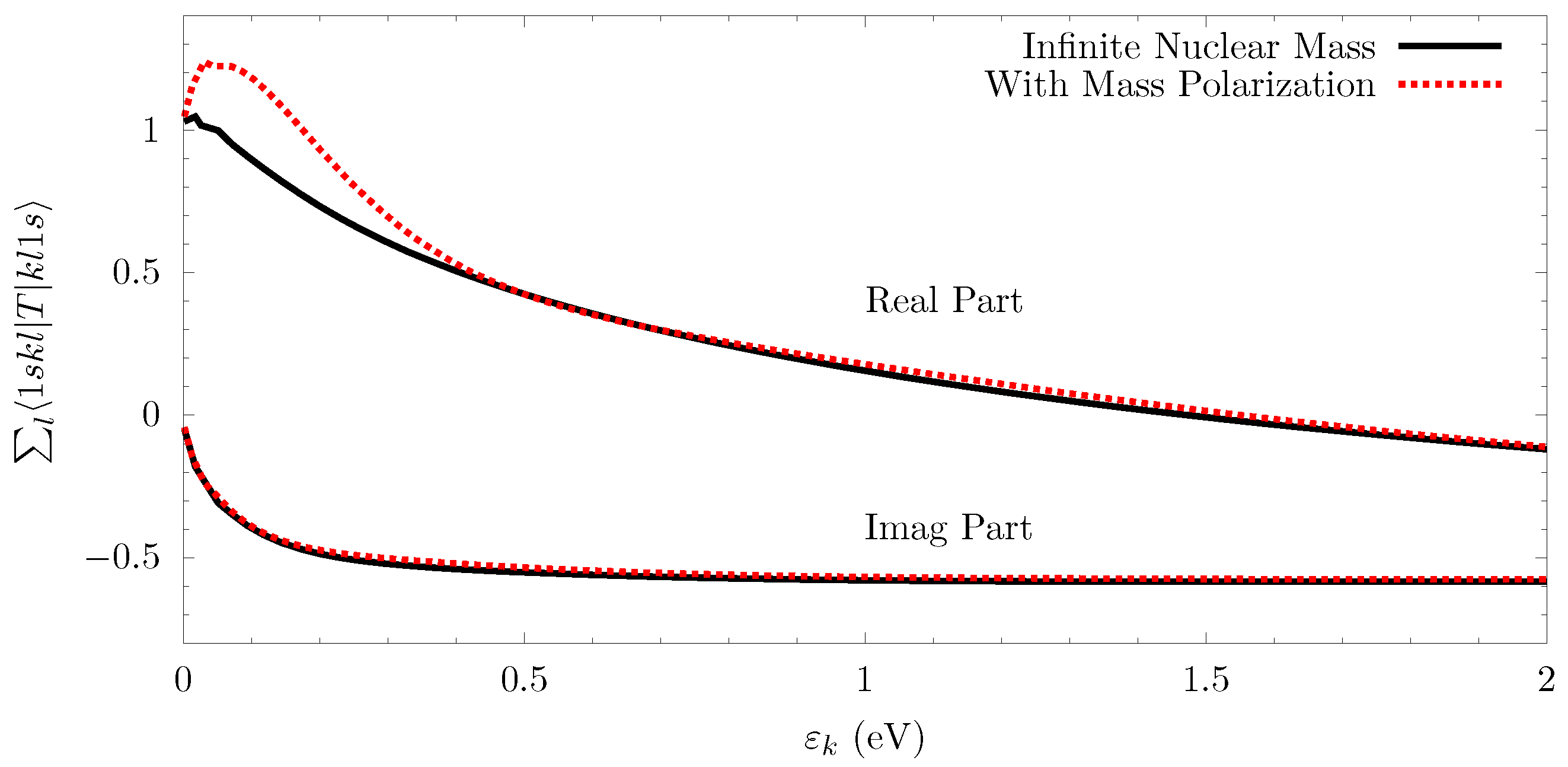
Spectral line shapes are used to diagnose parameters of white dwarfs and neutron stars in particular. In magnetized plasmas, the motion of the radiating atom in the plasma needs to be considered in the collision process as the electronic structure of the atom depends on its center-of-mass translational momentum. More broadly, collision models do not explicitly or fully account for the motion of the nucleus, accounting for deflection through conservation of momentum. Traditionally, the correlation between electronic and nuclear motion has been captured through mass-polarization terms involving momenta scalar products between different electrons. We reformulate the collision problem accounting for the motion of the nucleus, taking advantage of unitary transformations. In this new formulation, Coulomb interactions between the atom and projectile/plasma particle become displaced Coulomb interactions, and exchange interactions include corrections of order $1/M_A$. We demonstrate the resulting impact on the elastic scattering T-matrices of the $1s$ state of hydrogen, where the lowest-energy electrons increase the real part by 20–30% while leaving the imaginary part practically unaltered. Lastly, we present a formulation so that the atomic motion can be explicitly included in the collision problem for magnetic-field applications.

1. Introduction

Spectral line shapes are useful diagnostic tools in laboratory experiments as well as for diagnosing astrophysical parameters. For example, the gravity (and thus masses) of white dwarfs can be determined using spectroscopy by fitting measured spectra via a model atmosphere with Stark-broadened hydrogen lines (e.g., [1]). The study of the spectra of magnetized astrophysical objects is particularly important for both neutron star and white dwarf astrophysics.

For neutron stars, the equation of state—how the pressure, density, and temperature are related—of the dense matter found in neutron star interiors is unknown. Accurate neutron-star mass and radius determinations provide one of the strongest observational constraints on the dense-matter equation of state [2,3]. Since these quantities can be inferred spectroscopically [4], reliable line-shape models are essential for interpreting observations of strongly magnetized neutron-star atmospheres.

Magnetic white dwarfs (MWDs) are currently thought to be older and more massive [5,6] on average than their field-free counterparts. This implies that MWDs formed differently than non-magnetic white dwarfs. If correct, MWDs could be the product of mergers, although other explanations are that the magnetic fields come from hidden fields in the convective cores of the star, or that the field emerges as a result of crystallization. However, these mass estimates are derived from incomplete line-shape physics.

Work has only begun to perform line-shape calculations that include simultaneous pressure and magnetic-field broadening. The changes to the atomic structure are trivial regarding these line-shape calculations [7,8]. Recently, Rosato et al. [9] incorporated the helical motion of the plasma particles into the broadening problem. Gomez et al. [10] developed a quantum version of a line-shape formalism, including accounting for Pauli exclusion between plasma electrons and the radiating electron [11].

However, due to the nature of atomic physics in strong magnetic fields, the problem is more complicated than just splitting the atomic levels and having the plasma electron move on helical trajectories. It has been well established that, in magnetic fields, the electronic structure of atoms is directly impacted by the mechanical motion of atoms, a phenomenon called the motional Stark effect. There have been some attempts to try to include the motional Stark effect in line shapes. For example, Rosato [8] and Gomez et al. [12] found that the simultaneous interaction between plasma perturbations and the motional Stark effect is not trivial and can have competing effects. There is also a technical aspect that has prevented its inclusion in scattering problems: the matrix elements for the motional Stark effect for free electrons result in a Dirac delta function. Gomez et al. [13] reformulated the scattering problem for the motional Stark effect in magnetized problems, moving the delta function to be included in the Green function with the other singularities. However, this representation is not ideal for line-shape calculations and becomes increasingly difficult to generalize to more complicated systems.

Therefore an alternative formulation is needed to properly account for the nuclear/atomic motion during collisions between the radiating atom and plasma particles. While the greatest impact will be for the case of magnetized plasmas, the atomic motion is not zero in non-magnetized plasmas. Historically, conservation of momentum has been used to determine the amount of deflection from a collision. However, most collision problems do not account for the motion of the nucleus. While expected to be small, it is unknown how collisions alter the motion of the nucleus and how that translates to spectral line shapes.

In this work, we develop a scattering formalism that explicitly incorporates atomic and nuclear motion in both magnetic and non-magnetic plasmas. Using unitary transformations, we reformulate the Coulomb interaction such that mass-polarization and motional effects can be treated consistently within the scattering framework.

The rest of the paper is outlined as follows. Section 2 describes mass polarization, a phenomenon that arises for multi-electron problems. Section 3 outlines the traditional method for constructing the scattering problem and how to account for mass polarization in the Coulomb interactions within that framework. Section 4 discusses an alternate coordinate system that (with a unitary transform) completely removes the coupling of the nuclear motion from the projectile that extends to magnetic fields. Since unitary transformations are used to simplify scattering problems, in Section 5.1, we discuss the impact that these unitary transformations have on spectral line broadening. Finally, we extend the formalism to scattering in strong magnetic fields, where the coupling between atomic motion and internal structure becomes especially important.

2. Mass Polarization

For a multi-electron atom, it is well known that there are corrections to the atomic structure due to what is known as mass polarization; this does not occur in one-electron systems. The mass polarization arises from transformation of the momentum operators from a laboratory frame to a center-of-mass and relative-coordinate frame [14]. This arises as an inner product of the different electron momenta,

$${\displaystyle \frac{1}{m_n}}{\mathcal{p}}_i·{\mathcal{p}}_j,$$

(1)

where $m_n$ is the mass of the nucleus; $\mathcal{p}$ indicates the momentum operator in the center-of-mass frame where the subscripts i and j indicate different electrons.

In helium, when the two electrons move coherently, the nucleus recoils in response to their combined motion. Conversely, when the electronic motions oppose one another, the induced nuclear motion is reduced. The correction to the energy level structure of atoms is generally quite small. In ⁴He, for example, the correction to the ground state energy is $2.2\times {10}^{-5}$ hartree [14], a small correction but necessary in high-precision experiments. Consequently, nuclear motion is often neglected in conventional atomic-structure and collision calculations. However, in strong magnetic fields, where the atomic center-of-mass motion couples directly to the internal electronic structure, such approximations may no longer be sufficient.

3. Mass Polarization in Scattering

To incorporate nuclear recoil into the scattering formalism, we begin with the non-relativistic Hamiltonian of an N-electron atom plus a projectile in the “Laboratory Frame”,

$$H={\displaystyle \frac{1}{2m_n}}{p}_n^2+{\displaystyle \frac{1}{2m_e}}\sum _i{p}_i^2+\sum _i{V}_{in}+\sum _{ij}{V}_{ij}+{\displaystyle \frac{1}{2m_p}}{p}_p^2+V_{pn}+\sum _i{V}_{ip}$$

(2)

where the set of $V_{ij}$ are Coulomb interaction potentials between particles i and j; here particles $i, j$ are the electrons of the target electrons, p is the projectile particle and n designates the nucleus. To simplify the problem, the coordinates are transformed to the center-of-mass (CoM) and relative-coordinate representation (referred to as the CoM representation from here on out). The CoM and the relative coordinates of the atomic and projectile electrons are

$$\begin{array}{cc}\hfill R_{CM}& ={\displaystyle \frac{1}{M_A+m_p}}\left(m_p{r}_p+m_n{r}_n+\sum _i{m}_e{r}_i\right)\hfill \end{array}$$

(3)

$$\begin{array}{cc}\hfill {\mathcal{r}}_i& =r_i-r_n\hfill \end{array}$$

(4)

$$\begin{array}{cc}\hfill {\mathcal{r}}_p& =r_p-r_n,\hfill \end{array}$$

(5)

where $M_A=m_n+N{m}_e$ is the total mass of the atom and $m_p$ is the mass of the projectile. We will keep the mass of the projectile general for now. The resulting Hamiltonian is the familiar one presented for the He atom in Bethe and Salpeter [14]. The transformations of the momenta are

$$\begin{array}{cc}\hfill p_n& =P_{CM}{\displaystyle \frac{m_n}{M_A+m_p}}-\sum _i{\mathcal{p}}_i-{\mathcal{p}}_p\hfill \end{array}$$

(6)

$$\begin{array}{cc}\hfill p_i& =P_{CM}{\displaystyle \frac{m_e}{M_A+m_p}}+{\mathcal{p}}_i\hfill \end{array}$$

(7)

$$\begin{array}{cc}\hfill p_p& =P_{CM}{\displaystyle \frac{m_p}{M_A+m_p}}+{\mathcal{p}}_p.\hfill \end{array}$$

(8)

Collecting the various terms from the kinetic energy operator, we have the kinetic energy of the center of mass, the kinetic energies of the individual electrons and two mass polarization terms,

$$H=T_{CM}+H_{MP,A}+\sum _i{T}_i+\sum _i{V}_i^{\left(n\right)}+\sum _{ij}{V}_{ij}+T_p+V_p^{\left(n\right)}+\sum _i{V}_{ip}+H_{MP,p},$$

(9)

where $H_{MP,A}$ and $H_{MP,p}$ are the mass-polarization terms that couple the atomic electrons to each other and the atomic electrons to the projectile, respectively. These mass-polarization terms are defined explicitly as

$$H_{MP,A}={\displaystyle \frac{1}{m_n}}\sum _{i>j}{\mathcal{p}}_i·{\mathcal{p}}_j{H}_{MP,p}={\displaystyle \frac{1}{m_n}}\sum _i{\mathcal{p}}_i·{\mathcal{p}}_p.$$

(10)

The scattering problem solves the Lippmann–Schwinger equation [15], where the total scattered wave is given by

$${\displaystyle \left|{\mathsf{\Psi }}^{+}\right.〉=\left|\varphi \right.〉+\frac{1}{E-H_0}V\left|{\mathsf{\Psi }}^{+}\right.〉,}$$

(11)

where ${\displaystyle \left|\varphi \right.〉}$ are eigenstates of $H_0$, which is (not considering the CoM kinetic energy)

$$H_0=H_A+T_p,$$

(12)

and

$$H_A=\sum _i{T}_i+\sum _i{V}_i^{\left(n\right)}+\sum _{ij}{V}_{ij}+H_{MP,A}.$$

(13)

Each $T_i$ is the kinetic energy but with the reduced mass

$$T_i={\displaystyle \frac{1}{2{\mu }_e}}{\mathcal{p}}_i^2,$$

(14)

where ${\mu }_e=1/(m_n^{-1}+m_e^{-1})=m_n{m}_e/(m_n+m_e)$. V is the interaction potential between the atom and projectile, given by the terms

$$V=V_p^{\left(n\right)}+\sum _i{V}_{ip}+H_{MP,p};$$

(15)

where exchange matrix elements are omitted for brevity.

Rather than treating the projectile–target mass-polarization term directly, we instead seek a representation in which these couplings are absorbed into the interaction potential. This can be accomplished through a unitary transformation that shifts the projectile coordinate by the collective electronic coordinates of the target.

Matrix elements of the $H_{MP,p}$ will result in a delta function, complicating their incorporation into Equation (11) as part of the interaction potential between the atom and projectile. Therefore, to mitigate this, we will boost each of the target electrons by the scaled projectile momentum,

$$U=\exp \{i\mathfrak{m}{m}_n^{-1}{\mathcal{p}}_p·\sum _i{\mathcal{r}}_i\},$$

(16)

where c is a constant to be determined to completely cancel the mass-polarization terms between the projectile and the target electrons. This effectively adds the projectile momentum to the target electrons (although scaled by the mass of the nucleus). With this transformation, the projectile position is shifted by the positions of the other electrons

$$U{\mathcal{r}}_p{U}^{†}={\mathcal{r}}_p+{\displaystyle \frac{\mathfrak{m}}{m_n}}\sum _i{\mathcal{r}}_i,$$

(17)

while the ${\mathcal{r}}_i$ coordinates remain unchanged. The momentum of the projectile picks up terms of the atomic momenta,

$$U{\mathcal{p}}_i{U}^{†}={\mathcal{p}}_i-{\displaystyle \frac{\mathfrak{m}}{m_n}}{\mathcal{p}}_p.$$

(18)

The various momentum terms are modified:

$${\displaystyle \frac{1}{m_n}}\sum _{i>j}{\mathcal{p}}_i·{\mathcal{p}}_j\Rightarrow {\displaystyle \frac{1}{m_n}}\sum _{i>j}\left({\mathcal{p}}_i-{\displaystyle \frac{\mathfrak{m}}{m_n}}{\mathcal{p}}_p\right)·\left({\mathcal{p}}_j-{\displaystyle \frac{\mathfrak{m}}{m_n}}{\mathcal{p}}_p\right)$$

(19)

$${\displaystyle \frac{1}{m_n}}\sum _i{\mathcal{p}}_i·{\mathcal{p}}_p\Rightarrow {\displaystyle \frac{1}{m_n}}\sum _i\left({\mathcal{p}}_i-{\displaystyle \frac{\mathfrak{m}}{m_n}}{\mathcal{p}}_p\right)·{\mathcal{p}}_p$$

(20)

$${\displaystyle \frac{1}{2{\mu }_e}}{\mathcal{p}}_i^2\Rightarrow {\displaystyle \frac{1}{2{\mu }_e}}{\mathcal{p}}_i^2+{\displaystyle \frac{\mathfrak{m}}{2{\mu }_e{m}_n}}{\mathcal{p}}_p^2-{\displaystyle \frac{\mathfrak{m}}{{\mu }_e{m}_n}}{\mathcal{p}}_i·{\mathcal{p}}_p.$$

(21)

To remove all terms of the form ${\mathcal{p}}_i·{\mathcal{p}}_p$, then $\mathfrak{m}={[m_n^{-1}+{\mu }_e^{-1}]}^{-1}$. This shift causes the projectile to have a slightly different effective mass. The new reduced mass is

$$\begin{array}{cc}\hfill {\displaystyle \frac{1}{{\mu }_p^{\prime }}}& ={\displaystyle \frac{1}{{\mu }_p}}+{\displaystyle \frac{N\mathfrak{m}}{m_n}}\left[{\mu }_e^{-1}-2m_n^{-1}+N\mathfrak{m}{m}_n^{-2}\right]\hfill \end{array}$$

(22)

$$\begin{array}{cc}\hfill & \approx {\displaystyle \frac{1}{{\mu }_p}}+{\displaystyle \frac{N}{m_n}}\hfill \end{array}$$

(23)

to leading order in $m_n$, meaning that the projectile moves with a slightly lower effective mass.

This then shifts the mass polarization to the Coulomb interactions between the nucleus and target electrons, where

$$-{\displaystyle \frac{Z}{|{\mathcal{r}}_p|}}\Rightarrow -{\displaystyle \frac{Z}{|{\mathcal{r}}_p+\mathfrak{m}{m}_n^{-1}{\sum }_i{\mathcal{r}}_i|}}$$

(24)

and the electron–electron interaction becomes

$${\displaystyle \frac{1}{|{\mathcal{r}}_p-{\mathcal{r}}_i|}}\Rightarrow {\displaystyle \frac{1}{|{\mathcal{r}}_p-{\mathcal{r}}_i+\mathfrak{m}{m}_n^{-1}{\sum }_j{\mathcal{r}}_j|}}.$$

(25)

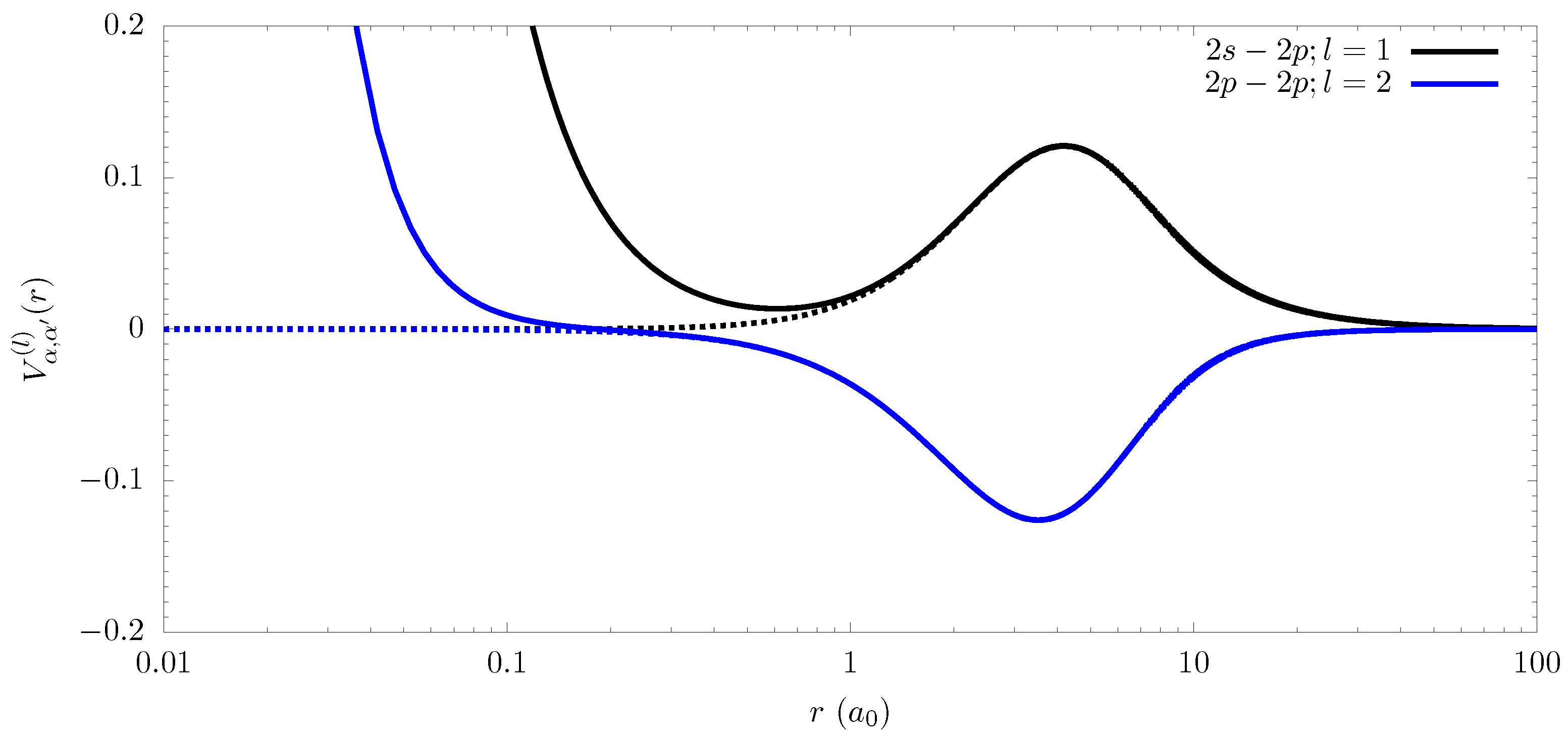
Now, the Coulomb interactions between the projectile and the target have an additional shifted component. The leading order of the nuclear term results in a singular part to the dipole term of the multipole expansion of the Coulomb interaction. Previously, only the monopole term carried a singular part near the origin. However, the dipole part is far weaker due to the $m_n^{-1}$ factor in the expansion. The expansion for one-electron systems is (assuming $m_n^{-1}{\mathcal{r}}_i$ is always small) given by

$$-{\displaystyle \frac{Z}{|{\mathcal{r}}_p+{\mu }_e{m}_n^{-1}{\sum }_i{\mathcal{r}}_i|}}\approx -Z\sum _i\sum _l{(-1)}^l{\displaystyle \frac{{\left({\mu }_e{m}_n^{-1}{r}_i\right)}^l}{r_p^{l+1}}}\sum _q{Y}_{lq}^{\ast }\left({\widehat{r}}_p\right)Y_{lq}\left({\widehat{r}}_i\right),$$

(26)

and is visualized in Figure 1.

One unfortunate complication of this procedure is that, while terms like ${\mathcal{p}}_i·{\mathcal{p}}_p$ have been eliminated, some of the complexities of mass polarization have been shifted to the exchange operator. $P_{01}$ swaps electron 0 and electron 1, where the former is the traditional label for the projectile and electrons 1…N are the target electrons. Applying the unitary transformation on this operator results in

$$U{P}_{01}{U}^{†}=\exp \left\{i\mathfrak{m}{m}_n^{-1}\left[({\mathcal{p}}_p-{\mathcal{p}}_1)·\sum _i{\mathcal{r}}_i+{\mathcal{p}}_1·{\mathcal{r}}_1-{\mathcal{p}}_1·r_p\right]\right\}{P}_{01},$$

(27)

which significantly complicates the evaluation of exchange matrix elements due to the resulting coupling between all electronic coordinates.

4. An Alternate Coordinate System: The Relative-Motion Representation

We want to explore an alternate coordinate system, the relative-motion representation, which simplifies some of the mass polarization physics considerably and lends itself to magnetic-field scattering. The relative-motion representation was introduced by Bezchastnov et al. [16] to calculate atomic structure of anions in high magnetic fields. This representation does not eliminate mass-polarization effects but redistributes them into modified interaction and exchange terms. As in the previous section, unitary transformations can remove mass-polarization term from the Hamiltonian.

Beginning with the atom’s CoM and relative coordinates, the projectile coordinate becomes that relative to the atom’s CoM,

$$\begin{array}{cc}\hfill {\mathcal{r}}_p& =r_p-R_A\hfill \end{array}$$

(28a)

$$\begin{array}{cc}\hfill {\mathcal{r}}_i& =r_i-r_n\hfill \end{array}$$

(28b)

$$\begin{array}{cc}\hfill R_A& ={\displaystyle \frac{1}{M_A}}(m_n{r}_n+m_e{\displaystyle \sum _{i=1}^N}{r}_i),\hfill \end{array}$$

(28c)

$$\begin{array}{cc}\hfill {\mathcal{R}}_A& =R_A\hfill \end{array}$$

(28d)

Under this system, the coordinates of the center of mass and relative motion are unchanged from their isolated-atom coordinates. The Coulomb interactions with the nucleus and the electrons automatically pick up their shifted Coulomb form

$$V_p^{\left(n\right)}={\displaystyle \frac{Z{q}_p}{|{\mathcal{r}}_p+\frac{m_e}{M_A}{\sum }_i{\mathcal{r}}_i|}}\mathrm{and}{V}_{ip}=-{\displaystyle \frac{q_p}{|{\mathcal{r}}_p-{\mathcal{r}}_i+\frac{m_e}{M_A}{\sum }_j{\mathcal{r}}_j|}},$$

(29)

with the mass being the total mass of the atom instead of the mass of the nucleus. As before, the evaluation of this operator proceeds as before in the CoM representation; details are given in Appendix A. The momentum of the CoM of the atom, however, picks up a term that includes the momentum of the projectile, while the projectile momentum keeps a similar form,

$$P_A\Rightarrow {\mathcal{P}}_T-{\mathcal{p}}_p\mathrm{and}{p}_p={\mathcal{p}}_p.$$

(30)

Here, we have labeled the new momentum that depends on the atom’s CoM as the total momentum, ${\mathcal{P}}_T$; this will become apparent after the unitary transformation. The mass polarization between the atom and the projectile becomes one that connects the projectile with the atom’s CoM momentum instead of the individual particles’ momenta,

$${\displaystyle \frac{1}{2{\mu }_p}}{\mathcal{p}}_p^2+{\displaystyle \frac{1}{2M_A}}{\mathcal{P}}_T^2-{\displaystyle \frac{1}{M_A}}{\mathcal{P}}_T·{\mathcal{p}}_p.$$

(31)

Since we will utilize unitary transforms, as we did before to rotate/shift the system, it is important to note that the new momentum operator commutes with the relative position operator

$$[{\mathcal{r}}_p,{\mathcal{P}}_T]=[r_p,P_A]-[R_A,P_A]+[r_p,p_p]-[R_A,p_p]=0.$$

(32)

Therefore, if we use unitary transformation

$$U=\exp \left\{-i{\displaystyle \frac{\mathfrak{m}}{M_A}}{\mathcal{P}}_T·{\mathcal{r}}_p\right\},$$

(33)

the mass-polarization terms can be eliminated. The resulting shift in the projectile momentum is

$$\begin{array}{c}\hfill U{\mathcal{p}}_p{U}^{-1}={\mathcal{p}}_p+\mathfrak{m}{M}_A^{-1}{\mathcal{P}}_T.\end{array}$$

(34)

In this transformation, the mass-polarization terms can be completely eliminated when $\mathfrak{m}={\mu }_p$. Since there are no residual terms of ${\mathcal{R}}_A$, there is no need to consider the resulting shift in the atom’s CoM position. There will be an additional term of ${\mu }_p{M}_A^{-1}{\mathcal{P}}_T^2$ that arises from the cross term in Equation (31). Combining the various mass terms in the kinetic energy of ${\mathcal{P}}_T$ results in the system having $M_T^{-1}=[1-{\mu }_p/M_A]/M_A$, where $M_T=m_p+M_A$, i.e., the total mass. Thus the final kinetic energy term is

$${\displaystyle \frac{1}{2{\mu }_p}}{\mathcal{p}}_p^2+{\displaystyle \frac{1}{2M_T}}{\mathcal{P}}_T^2.$$

(35)

The total momentum ${\mathcal{P}}_T^2$ now no longer appears anywhere else in the Hamiltonian and the atomic electron and projectile motions are independent of ${\mathcal{P}}_T$.

4.1. Exchange

Upon the interchange of electrons, the total wavefunction is

$$\begin{array}{c}{P}_{01}\mathsf{\Psi }({\mathcal{R}}_A,{\mathcal{r}}_p,{\mathcal{r}}_1,{\mathcal{r}}_2,\dots ,{\mathcal{r}}_N)\propto \hfill \\ \mathsf{\Psi }\left({\mathcal{R}}_A+{\displaystyle \frac{m_e}{M_A}}({\mathcal{r}}_p-{\mathcal{r}}_1),{\displaystyle \frac{m_n{\mathcal{r}}_1}{M_A}}-{\displaystyle \frac{m_e{\mathcal{r}}_p}{M_A}},{\mathcal{r}}_p+{\displaystyle \frac{m_e{\mathcal{r}}_1}{M_A}},{\mathcal{r}}_2,\dots ,{\mathcal{r}}_N\right),\hfill \end{array}$$

(36)

which is substantially more complicated than in the CoM representation in Section 3 before the unitary transformation. This is due to all electrons having the same reference point in Section 3 (before the unitary transformation), which results in the electrons simply switching coordinates.

When the electrons switch places, then the atomic CoM motion contributes a difference in coordinates into the matrix element. Fortunately though, our unitary transformation transforms the exchange operator so that

$${\tilde{P}}_{01}=U{P}_{01}{U}^{†}=\exp \left\{-i{\displaystyle \frac{\mathfrak{m}}{M_A}}{\mathcal{P}}_T·({\mathcal{r}}_p-{\mathcal{r}}_1)\right\}{P}_{01}.$$

(37)

Since the solution of the atomic CoM is a plane wave, ${\mathcal{V}}^{-1/2}\exp \left\{iK{\mathcal{R}}_A\right\}$, then this unitary transformation almost completely cancels the exchange-induced shift of the atomic CoM coordinate arising from the mixed coordinate representation, i.e.,

$$\begin{array}{c}{\tilde{P}}_{01}{\mathsf{\Psi }}_U({\mathcal{R}}_A,{\mathcal{r}}_p,{\mathcal{r}}_1,{\mathcal{r}}_2,\dots ,{\mathcal{r}}_N)\propto \hfill \\ e^{i{\displaystyle \frac{m_e-\mathfrak{m}}{M_A}}K·({\mathcal{r}}_p-r_1)}{\mathsf{\Psi }}_U\left({\mathcal{R}}_A,{\displaystyle \frac{m_n{\mathcal{r}}_1}{M_A}}-{\displaystyle \frac{m_e{\mathcal{r}}_p}{M_A}},{\mathcal{r}}_p+{\displaystyle \frac{m_e{\mathcal{r}}_1}{M_A}},{\mathcal{r}}_2,\dots ,{\mathcal{r}}_N\right)\hfill \end{array}$$

(38)

where the residual phase contributes for ${\mathcal{r}}_p$ only at $\mathcal{O}\left(M^{-2}\right)$. This then implies that the exchange of particles depends on the motion of the atom, but, even for a hydrogen atom, this would only occur at temperatures greater than ${10}^5$ eV, so it can be safely neglected. The advantage of this form and with Equation (37) is that the swap of coordinates only involves the two electrons in the ${\tilde{P}}_{01}$ operator, as opposed to Equation (27), which has all N electrons in ${\tilde{P}}_{01}$, which requires careful bookkeeping.

4.2. Exchange Matrix Elements

To calculate the correction that mass polarization has on overlap integrals—used for example on energy terms of the exchange operator, $E{P}_{01}$—performing a Taylor expansion will give us the lowest-order correction. This expansion is convenient because the wavefunction of the projectile with the target is a product form. Therefore, the lowest-order correction becomes

$$\begin{array}{c}{\mathsf{\Psi }}_U\left(R,{\displaystyle \frac{m_n{\mathcal{r}}_1}{M_A}}-{\displaystyle \frac{m_e{\mathcal{r}}_p}{M_A}},{\mathcal{r}}_p+{\displaystyle \frac{m_e{\mathcal{r}}_1}{M_A}},{\mathcal{r}}_2,\dots ,{\mathcal{r}}_N\right)\approx \hfill \\ \hfill \left[1+{\displaystyle \frac{m_e}{M_A}}({\mathcal{r}}_1·{\overrightarrow{\nabla }}_p-{\mathcal{r}}_p·{\overrightarrow{\nabla }}_1)\right]{\mathsf{\Psi }}_U\left(R,{\displaystyle \frac{m_n{\mathcal{r}}_1}{M_A}},{\mathcal{r}}_p,{\mathcal{r}}_2,\dots ,{\mathcal{r}}_N\right),\end{array}$$

(39)

which can be obtained using the same mathematical machinery as the traditional way of evaluating $V_{01}{P}_{01}$ (i.e., without mass-polarization corrections), where the resulting operator corrections are a rank 0 tensor made of a product of two rank 1 tensors,

$${\displaystyle \frac{m_e}{M_A}}({\mathcal{r}}_1·{\overrightarrow{\nabla }}_p-{\mathcal{r}}_p·{\overrightarrow{\nabla }}_1)$$

(40)

where each gradient operator can be expressed using spherical harmonics,

$${\displaystyle \langle l^{\prime }\parallel \overrightarrow{\nabla }\parallel l\rangle =\langle l^{\prime }\parallel C^{\left(1\right)}\parallel l\rangle \left\{\begin{array}{cc}{\displaystyle \frac{d}{dr}-\frac{l}{r}}\hfill & \mathrm{if}{l}^{\prime }=l+1\hfill \\ {\displaystyle \frac{d}{dr}+\frac{l+1}{r}}\hfill & \mathrm{if}{l}^{\prime }=l-1\hfill \end{array}\right..}$$

(41)

This has some interesting consequences for exchange. The correction in Equation (37) involves a tensor of rank 0 that is a scalar product of two rank 1 tensors. Higher-order corrections will involve tensors operators of higher rank. In the infinite mass approximation, $P_{01}$ involves only rank 0 tensors.

4.3. Numerical Example

We implemented all the modifications above to include nuclear motion in collisions. The changes are not expected to be big since $m_e/M_A\approx 1/1836$ for hydrogen. In our tests, we found that there are some numerical instabilities in the form of a resonance that moves with changing the Green function momentum-space grid.

In our tests using the Balrog code [17], the inclusion of mass polarization did not result in significant changes in excited state T-matrices. We specifically use the Balrog code because it has been demonstrated to satisfy the optical theorem to within machine precision. Since the optical theorem is a direct consequence of the scattering S-matrices obeying $S{S}^{†}=I$, then these calculations satisfy unitarity. The most significant changes were for the elastic T-matrices of the ground state, $1s$ of hydrogen, shown in Figure 2. Here, the inclusion of mass polarization resulted in different behavior for the lowest projectile energy (below $0.5$ eV). The biggest change is in the real part, where, at 0.1 eV, the total real part increased by 30%. The imaginary part (a proxy for the collision cross-section through the optical theorem) remains relatively unchanged compared to the real part. The high-energy parts of the T-matrices are practically identical.

Due to the general interest in the isolated line problem (e.g., [18,19,20,21,22]), we also examined the impact on the B iii $2s$-$2p$ transition. The change in the total T-matrices rarely exceeded 1%, with the area around resonances exhibiting larger changes, while the average change was ≲0.1% for both the real and imaginary parts, rising to 0.3% at the lowest energies. Including nuclear motion reduced the line width by 0.4%. For a line like Ne viii $3s$-$3p$, the line width increased by 0.01% in the conditions of the experiments of Glenzer et al. [18].

5. Impact on Spectral Line Broadening

It is well established that spectral line broadening is closely related to collisions [23,24]. In this section, we examine how the transformations developed in the previous sections modify the interpretation of spectral line broadening. We show how standard phenomenological models, including Doppler shifts induced by collisions and the $\mu$-ion model, arise naturally within this framework while also identifying additional corrections.

For some preliminaries, to calculate a line shape, we evaluate the real part of the Fourier transform of the thermal average of the atom’s dipole autocorrelation function [24,25],

$$I\left(\omega \right)=\Re {\pi }^{-1}{\int }_0^{\infty }dt{e}^{i\omega t}\mathrm{Tr}\left\{DD\left(t\right)\rho \right\}$$

(42)

where, in the Heisenberg representation,

$$D\left(t\right)=e^{iHt}D{e}^{-iHt}.$$

(43)

The density matrix, $\rho$, is often taken to be a Boltzmann,

$$\rho ={\displaystyle \frac{e^{-\beta H}}{\mathrm{Tr}{e}^{-\beta H}}},$$

(44)

although it is common practice to ignore the atom–plasma terms, making density matrix factorizable in the atom and plasma particle subspaces,

$$\rho \approx {\rho }_a{\rho }_p.$$

(45)

The factorized density matrix approximation is valid near the line center and is therefore often a good approximation [23,24,26].

5.1. How Unitary Transformations Affect Spectral Line Broadening

In the previous sections, we utilized unitary transformations to modify the collision problem. We will now explore how those unitary transformations affect Equation (42). The unitary transformation is included between all operators

$$\begin{array}{cc}\hfill \mathrm{Tr}\left\{DD\right(t\left)\rho \right\}& =\mathrm{Tr}\left\{D{U}^{†}U{e}^{iHt}{U}^{†}UD{U}^{†}U{e}^{-iHt}{U}^{†}U\rho U^{†}U\right\}\hfill \\ \hfill & =\mathrm{Tr}\left\{D{U}^{†}{e}^{i{H}_{U}t}UD{U}^{†}{e}^{-i{H}_{U}t}{\rho }_{U}U\right\}\hfill \\ \hfill & =\mathrm{Tr}\left\{D_U{e}^{i{H}_{U}t}{D}_U{e}^{-i{H}_{U}t}{\rho }_U\right\},\hfill \end{array}$$

(46)

where we have used the cyclical property of the trace. Because the electron dipole moment commutes with the unitary transformation, we were able to eliminate any lingering factors of U. This result means that the rest of the calculation can proceed using ${\displaystyle \left|{\psi }_U\right.〉}$ as the basis set. Further, once the Liouville notation is set up, it will drop completely from the evaluation of the T-matrices that make up the electron broadening operator.

This result is rather unremarkable as it essentially states that a rotation of the frame does not result in a change in the broadening. Therefore, transforming either the perturbing particle or the atomic target results in an identical broadening expression to that of a stationary atomic target.

5.2. How Atomic Deflection Changes Line Broadening

In the framework we have given here, we can explicitly account for the recoil of the atom as a result of the collision. Since the velocity of the atom changes as a result of the collision, then it would make sense that the Doppler shift of an individual atom will likewise change. The way to account for this is to use the Liouville formalism, where the Liouville operator acts on other operators, i.e., a tetradic superoperator [24],

$$\begin{array}{c}\hfill LO=[H,O],\end{array}$$

(47)

where O is an arbitrary operator. The Liouville operator offers a convenient shorthand for describing the time evolution of quantum systems. For example, the expression for the line shape can be written compactly as

$$\begin{array}{c}\hfill \mathrm{Tr}D{e}^{-iHt}\rho D{e}^{iHt}=\mathrm{Tr}D{e}^{-iLt}\rho D\end{array}$$

(48)

where the left-hand side is obtained from Equation (42) through the cyclical invariance of the trace. After the evaluation of the time integral, the line-shape equation is defined as

$$\begin{array}{c}\hfill I\left(\omega \right)=\mathrm{Tr}DR\left(\omega \right)\rho D,\end{array}$$

(49)

where the resolvent operator is defined as

$$\begin{array}{cc}\hfill R\left(\omega \right)& =\delta (\omega -L)\hfill \\ \hfill & =-{\displaystyle \frac{\Im }{\pi }}{\displaystyle \frac{1}{\omega -L}},\hfill \end{array}$$

and, in the latter expression, there is an implied small imaginary part to ensure the convergence of the integral; it is assumed that the limit as this number approaches zero will be taken.

In the Liouville formalism, the operator contains the Liouville operators of the individual systems and the interaction between them,

$$\begin{array}{c}\hfill L=L_0^a+L_0^p+L_I.\end{array}$$

(50)

Here, the 0 subscript denotes operators that do not contain interactions between systems. In other words, the $L_0^a$ can describe interactions between two atomic electrons but not those electrons with the plasma system.

To include the Doppler shift within the Liouville formalism, we assume the observer is stationary. The expression for the Doppler shift is given (classically) as

$$\mathsf{\Delta }\omega =\overrightarrow{\mathbf{e}}·\overrightarrow{v}{\displaystyle \frac{1}{c}}{\omega }_0,$$

(51)

where c here is the speed of light and $\overrightarrow{\mathbf{e}}$ ensures that only velocities in the direction of the observer produce a shift, and ${\omega }_0$ is the frequency of the radiation with no motion or in the frame of the radiator. We will then express this quantum mechanically by writing this as

$$L_{\mathrm{Dopp}}=\left({\displaystyle \frac{1}{c{M}_A}}\overrightarrow{\mathbf{e}}·\overrightarrow{P_A}\right){\omega }_0.$$

(52)

Alternatively, we can express the Doppler shift in terms of a Liouville operator and a reference velocity,

$$L_{\mathrm{Dopp}}=\left(\overrightarrow{\mathbf{e}}·{\overrightarrow{v}}_A+L_{A,D}\right){\omega }_0,$$

(53)

where

$$\begin{array}{c}\hfill L_{A,D}O={\displaystyle \frac{1}{c{M}_A}}[\overrightarrow{\mathbf{e}}·{\overrightarrow{P}}_A,O].\end{array}$$

(54)

If there is no change in the atom’s velocity, then $L_{A,D}$ is zero.

Using the transformations described above, the momentum operator becomes shifted where

$$P_{A,\Vert }\Rightarrow {\mathcal{P}}_{T,\Vert }-{\mathcal{p}}_{p,\Vert }.$$

(55)

Then, after the unitary transformations, ${\mathcal{P}}_T$ becomes a constant of motion and can be ignored for the rest of the problem. There are complications with evaluating the momentum operator for free states. Therefore, we outline several methods for evaluation in Appendix B. Since the momentum operator is a tensor of rank 1 and the line broadening involves a trace of the plasma electron coordinates, then the lowest-order correction will be second order in the momentum operator. Therefore, whatever the broadening is that comes from this correction will be of order $\mathcal{O}\left({\left(Mc\right)}^{-2}\right)$.

5.3. The $\mu$-Ion Model for Line-Shape Simulations

Many simulation line-shape calculations [27,28,29,30] use trivial particle motions, meaning that plasma correlations are neglected, usually to be corrected for by screening the interaction potential. These models often use the so-called $\mu$-ion model, where the plasma electrons and ions move with the effective mass being equal to the reduced mass. For electrons, this hardly results in any change, but, for ions, this can change the motion of particles quite substantially. Although typically introduced heuristically in simulation approaches, we show here that the $\mu$-ion model arises naturally from a transformation to the radiator-centered (relative) frame.

In an N-particle plasma, we have the target/atomic Hamiltonian,

$$H_A={\displaystyle \frac{1}{2M_A}}{P}_A^2+h_A$$

(56)

where $h_A$ represents the internal electronic coordinates of the atomic Hamiltonian but also those of the remaining particles and their interaction with the target atom and their interactions among each other,

$$H=H_A+\sum _i{\displaystyle \frac{1}{2m_i}}{p}_i^2+V_{iA}+\sum _j{V}_{ij}.$$

(57)

The atom’s CoM momentum transforms to include all particles,

$$P_A\Rightarrow {\mathcal{P}}_T-\sum _i{\mathcal{p}}_i.$$

(58)

Further, using the unitary boost described above in Equation (33) results in all plasma kinetic energy terms being

$${\displaystyle \frac{1}{2M_A}}\left(1-{\displaystyle \frac{{\sum }_i{\mu }_i}{M_A}}\right){\mathcal{P}}_T^2+\sum _i{\displaystyle \frac{1}{2{\mu }_i}}{\mathcal{p}}_i^2-\sum _{i>j}{\displaystyle \frac{1}{M_A}}{\mathcal{p}}_j·{\mathcal{p}}_i.$$

(59)

Therefore, in the end, the motion of the radiator is factored out and does not appear in the Hamiltonian anymore. Further, all particles move with the reduced mass relative to the radiator, in line with the $\mu$-ion model currently in use in simulation codes such as Xenomorph [30], SimU [29], etc. [27,31]. The dynamics of screening are unchanged from the lab frame. The only missing pieces from the current simulation codes are the kinetic energy cross terms.

Further use of unitary transformations can be made to transform the cross terms. Applying the unitary transformation

$$U=\exp \{-i\sum _{i,j\ne i}{\mu }_i{M}_A^{-1}{\mathcal{p}}_j·r_i\},$$

(60)

the kinetic energy terms involving the relative particle momenta are transformed so that

$$\sum _i{\displaystyle \frac{1}{2{\mu }_i}}{\mathcal{p}}_i^2\Rightarrow \sum _i{\displaystyle \frac{1}{2{\mu }_i}}{\mathcal{p}}_i^2+\sum _{i,j\ne i}{\displaystyle \frac{1}{M_A}}{\mathcal{p}}_j·{\mathcal{p}}_i+\sum _i{\displaystyle \frac{{\mu }_i}{2M_A^2}}{\left(\sum _{j\ne i}{\mathcal{p}}_j\right)}^2,$$

(61)

and

$$-\sum _{i,j\ne i}{\displaystyle \frac{1}{M_A}}{\mathcal{p}}_j·{\mathcal{p}}_i\Rightarrow -\sum _{i,j\ne i}{\displaystyle \frac{1}{M_A}}{\mathcal{p}}_j·{\mathcal{p}}_i-\sum _i{\displaystyle \frac{{\mu }_i}{M_A^2}}{\left(\sum _{j\ne i}{\mathcal{p}}_j\right)}^2.$$

(62)

This does not completely remove all mass-polarization terms between plasma particles but shifts them so that they are weighted by $M_A^{-2}$ instead of $M_A^{-1}$. The Coulomb interactions between particles are slightly modified so that, between two plasma particles, the Coulomb interactions become

$${\displaystyle \frac{q_i{q}_j}{|{\mathcal{r}}_i-{\mathcal{r}}_j|}}\Rightarrow {\displaystyle \frac{q_i{q}_j}{|{\mathcal{r}}_i(1+{\mu }_i{M}_A^{-1})-{\mathcal{r}}_j(1+{\mu }_j{M}_A^{-1})|}},$$

(63)

which in effect means that the plasma particles are slightly farther away from each other, having a weaker Coulomb interaction between them. The more interesting Coulomb interaction is between the target and the plasma particles. The transformed Coulomb interaction is (omitting position operator terms from the atom of order $m_e/M_A^{-1}$)

$${\displaystyle \frac{q_p}{|{\mathcal{r}}_p-{\mathcal{r}}_a|}}\Rightarrow {\displaystyle \frac{q_p}{|{\mathcal{r}}_p-{\mathcal{r}}_a-{\sum }_{j\ne p}{\mu }_j{M}_A^{-1}{\mathcal{r}}_j|}},$$

(64)

where the subscripts p and a correspond to the plasma particle and an atomic electron. There will be a similar expression for the interaction between the nucleus and the plasma particle. The result (not surprising) is that the interaction between the atom and plasma particles is given by a displaced Coulomb interaction. However, this time, the displacement is by the collective plasma; this is separate from screening. Some preliminary examination suggests that this will result in modified screening but will be related to mass screening, with more weight given to massive particles in the plasma. For an exactly isotropic plasma, a thermal average suggests that ${\sum }_j{r}_j$ should be zero. Since plasmas are perfectly isotropic in the average, the corrections here, therefore, would be non-zero whenever the plasma in the vicinity of the target atom is not perfectly isotropic. However, we will not provide further interpretation or a prescription to incorporate this correction.

6. Atomic Motion in Collisions with Particles in High Magnetic Field

In a magnetic field, the kinetic energy operators are now severely complicated by the presence of a magnetic field. As has been well established (e.g., [32,33]), the motion of the atom depends on the internal motion of the atom’s electron(s) and nucleus. Further, there are three different types of momenta to consider. The first is the canonical momentum, $p=-i\overrightarrow{\nabla }$, which is used in non-magnetic applications. The second is the kinetic momentum, $\pi =p-eA\left(r\right)$, and is the true motion of a particle. Last is the pseudomomentum, $k=\pi +e(B\times r)$, which is a constant of the particle motion and is closely related to the guiding center of a particle. In the absence of a magnetic field, all momenta are equal to the canonical momentum. For the remainder of this section, we adopt the symmetric gauge; i.e.,

$$\begin{array}{c}\hfill A\left(r\right)={\displaystyle \frac{1}{2}}B\times r.\end{array}$$

(65)

In the scattering problem, it is convenient to separate the atomic and projectile motion without interaction. If we set up the scattering problem using the total system’s CoM, like in Section 3, then the atomic structure now depends on the motion of the projectile, with eigenstates in the absence of interaction of both the projectile and the target atom’s electron depending on the CoM of the entire coupled system. Even using the relative-coordinate representation in Section 4 does not fix this problem; see results of Bezchastnov et al. [16] and Bezchastnov et al. [34].

Therefore, since adding a projectile electron before there is any interaction with the projectile alters the atomic structure, a new formulation is required.

6.1. Neutral Radiator

We will now address the case where there is a strong magnetic field for a neutral. The most convenient form will be to use the relative coordinates. We begin with the already established results in (28), where

$$\begin{array}{cc}\hfill {\mathcal{r}}_p& =r_p-R_A\hfill \\ \hfill {\mathcal{r}}_i& =r_i-r_n\hfill \\ \hfill R_A& ={\displaystyle \frac{1}{M_A}}(m_n{r}_n+m_e{\displaystyle \sum _{i=1}^N}{r}_i),\hfill \\ \hfill {\mathcal{R}}_A& =R_A\hfill \end{array}$$

and, with a magnetic field, the kinetic momenta are

$$\begin{array}{cc}\hfill {\pi }_p& ={\mathcal{p}}_p+{\displaystyle \frac{e}{2}}B\times {\mathcal{R}}_A+{\displaystyle \frac{e}{2}}B\times {\mathcal{r}}_p\hfill \end{array}$$

(66a)

$$\begin{array}{cc}\hfill {\pi }_A& \Rightarrow {\mathcal{P}}_A-{\mathcal{p}}_p-B\times r_A.\hfill \end{array}$$

(66b)

So far, this follows the setup of Bezchastnov et al. [16] and Bezchastnov et al. [34]. However, the matrix elements of motional Stark terms for free particles are delta functions. Further, applying the unitary transform $U=\exp \{(i/2)(B\times {\mathcal{p}}_p)·\mathcal{R}\}$ fully entangles the projectile motion with that of the atom, thus eliminating any sense of isolated-atom atomic structure as part of the scattering problem; this makes any evaluation of scattering amplitudes inherently difficult. If we apply the same unitary transformation as in Section 4—but only in the z-direction—and boost the atomic momenta by the canonical momentum of the projectile,

$$U=\exp \left\{-i{\mathcal{p}}_p·{\mathcal{R}}_{A,\perp }-i{\mu }_p{M_A}^{-1}{\mathcal{P}}_{A,\Vert }·{\mathcal{r}}_{p,\Vert }\right\},$$

(67)

we obtain the following shifts:

$$\begin{array}{cc}\hfill {\mathcal{r}}_p& \Rightarrow {\mathcal{r}}_p-{\mathcal{R}}_{A,\perp }\hfill \end{array}$$

(68a)

$$\begin{array}{cc}\hfill {\mathcal{P}}_A& \Rightarrow {\mathcal{P}}_A+{\mathcal{p}}_{p,\perp }\hfill \end{array}$$

(68b)

$$\begin{array}{cc}\hfill {\mathcal{p}}_p& \Rightarrow {\mathcal{p}}_p+{\mu }_p{M}_A^{-1}{\mathcal{P}}_{A,\Vert },\hfill \end{array}$$

(68c)

where ${\mu }_p={[m_p^{-1}+M^{-1}]}^{-1}$; we have ignored the shifts in ${\mathcal{R}}_A$ since it only applies in the direction aligned with the field and that appears nowhere in the current form of the Hamiltonian. This shift ultimately leaves a convenient form for both the projectile and atomic kinetic momenta,

$${\pi }_p={\mathcal{p}}_p+{\mu }_p{M}_A^{\prime -1}{\mathcal{P}}_{A,\Vert }+{\displaystyle \frac{e}{2}}B\times {\mathcal{r}}_p\mathrm{and}{\pi }_A=(1-{\mu }_p{M}_A^{-1}){\mathcal{P}}_{A,\Vert }+{\mathcal{P}}_{A,\perp }-{\mathcal{p}}_{p,\Vert }-B\times r_A,$$

(69)

which makes the total kinetic energy

$${\displaystyle \frac{1}{2M_A^{\prime }}}{\mathcal{P}}_{\Vert }^2+{\displaystyle \frac{1}{2M}}{\left[{\mathcal{P}}_{A,\perp }-(B\times r_A)\right]}^2+{\displaystyle \frac{1}{2\mu }}{\mathcal{p}}_{p,\Vert }^2+{\displaystyle \frac{1}{2m_e}}{\left(p_{p,\perp }+{\displaystyle \frac{e}{2}}B\times {\mathcal{r}}_p\right)}^2,$$

(70)

where $M_A^{\prime }=M_A/[1-(1-m_p/{\mu }_p){\mu }_p/M_A+{\left({\mu }_p/M_A\right)}^2]$. This form sufficiently separates any entanglement of momenta and removes any coupling between the projectile and atom, which includes the motional Stark effect while retaining the original structure of the atom.

However, this has the unfortunate property that the Coulomb interactions become dependent on ${\mathcal{R}}_A$. This can be evaluated using the Fourier form of the Coulomb interaction between two electrons,

$${\displaystyle \frac{1}{|{\mathcal{r}}_p-{\mathcal{R}}_{A,\perp }-{\mathcal{r}}_i|}}={\displaystyle \frac{4\pi }{{\left(2\pi \right)}^3}}\int {\displaystyle \frac{d^{3}k}{k^2}}\exp \{i\overrightarrow{k}·[{\mathcal{r}}_p-{\mathcal{r}}_i-{\mathcal{R}}_{A,\perp }]\},$$

(71)

where we have (for now) neglected the additional terms of order $m_e/M_A$ for simplicity. We immediately perform the integral over $k_z$ to obtain the form in terms of the perpendicular k integral,

$${\displaystyle \frac{1}{|{\mathcal{r}}_p-{\mathcal{R}}_{A,\perp }-{\mathcal{r}}_i|}}=\int {\displaystyle \frac{d^2{k}_{\perp }}{2\pi }}{k}_{\perp }^{-1}\exp \{i{k}_{\perp }·[{\mathcal{r}}_{p,\perp }-{\mathcal{r}}_{i,\perp }-{\mathcal{R}}_{A,\perp }]\}\exp \{-k_{\perp }|{\mathcal{r}}_{p,\Vert }-{\mathcal{r}}_{i,\Vert }\left|\right\}.$$

(72)

Since the wavefunction of a neutral system includes a modified plane wave [33], for example

$$\mathsf{\Psi }({\mathcal{R}}_A,{\mathcal{r}}_i)={\left(2\pi \right)}^{-3/2}\exp \left\{i(K+{\displaystyle \frac{e}{2}}B\times {\mathcal{r}}_i)·{\mathcal{R}}_A\right\}\varphi \left({\mathcal{r}}_i\right)$$

(73)

for a one-electron system, then the evaluation of the matrix element involves a delta function. For given specific states of the neutral atom pseudomomenta, the matrix element of the Coulomb interaction becomes

$${\displaystyle \langle K\left|\right|{\mathcal{r}}_p-{\mathcal{R}}_{A,\perp }-{\mathcal{r}}_i{|}^{-1}|K^{\prime }\rangle =\frac{1}{2\pi }{k}_{\perp }^{-1}{e}^{i{\overrightarrow{k}}_{\perp }·({\mathcal{r}}_{p,\perp }-{\mathcal{r}}_{i,\perp })}{e}^{-|k_{\perp }\left|\right|{\mathcal{r}}_{p,\Vert }-{\mathcal{r}}_{i,\Vert }|},}$$

(74)

$${\displaystyle \sum _p\langle K\left|\right|{\mathcal{r}}_p-{\mathcal{R}}_{A,\perp }-{\mathcal{r}}_i{|}^{-1}|K^{\prime }\rangle =\frac{1}{2\pi }{k}_{\perp }^{-1}\left[\sum _p{e}^{i{\overrightarrow{k}}_{\perp }·{\mathcal{r}}_{p,\perp }}{e}^{-i{\overrightarrow{k}}_{\perp }·{\mathcal{r}}_{i,\perp }}{e}^{-|k_{\perp }\left|\right|{\mathcal{r}}_{p,\Vert }-{\mathcal{r}}_{i,\Vert }|}\right],}$$

(75)

$${\displaystyle \sum _p\langle K\left|\right|{\mathcal{r}}_p-{\mathcal{R}}_{A,\perp }-{\mathcal{r}}_i{|}^{-1}|K^{\prime }\rangle \approx \frac{1}{2\pi }{k}_{\perp }^{-1}\left[\sum _p{e}^{i{\overrightarrow{k}}_{\perp }·{\mathcal{r}}_{p,\perp }}{e}^{-|k_{\perp }\left|\right|{\mathcal{r}}_{p,\Vert }|}\right]e^{-i{\overrightarrow{k}}_{\perp }·{\mathcal{r}}_{i,\perp }}{e}^{|k_{\perp }\left|\right|{\mathcal{r}}_{i,\Vert }|},}$$

(76)

where ${\overrightarrow{k}}_{\perp }={\left(\mathsf{\Delta }{\overrightarrow{K}}_A\right)}_{\perp }$. If the potential is screened, then $k_{\perp }^2={\left(\mathsf{\Delta }{K}_A\right)}_{\perp }^2+k_{\mathrm{scr}}^2$. In problems involving a magnetic field, it becomes useful to expand the perpendicular plane wave. The cylindrical decomposition of the Coulomb interaction is in terms of Bessel functions,

$${\displaystyle \frac{1}{2\pi }}{k}_{\perp }^{-1}{e}^{-k_{\perp }·|z_p-z_i|}\sum _{q{q}^{\prime }}{i}^{q-q^{\prime }}{J}_q\left(k_{\perp }{\rho }_p\right)J_{q^{\prime }}\left(k_{\perp }{\rho }_i\right)e^{i[q{\varphi }_p-q^{\prime }{\varphi }_i-{\varphi }_K(q-q^{\prime })]}.$$

(77)

There will be a similar expression for the projectile–nuclear term (neglecting terms of order $m_e/M_A$, and $Z=1$),

$$V_p^{\left(n\right)}\approx -{\displaystyle \frac{1}{2\pi }}{k}_{\perp }^{-1}{e}^{-k_{\perp }\left|z_p\right|}\sum _q{i}^q{J}_q\left(k_{\perp }{\rho }_p\right)e^{iq({\varphi }_p-{\varphi }_K)}$$

(78)

which, combined with the projectile–nuclear term, makes the total interaction between the neutral atom and the projectile finite even as ${\left(\mathsf{\Delta }K\right)}_{\perp }\to 0$.

For both the projectile–electron and projectile–nucleus interactions, the Coulomb interaction is distorted and does not obey the usual selection rules for cylindrical symmetry. In Refs. [10,35,36], where the motional Stark effect is the only place nuclear motion appears in the Hamiltonian, then only $q=q^{\prime }$ is considered, and therefore only the absolute value of q is needed in the evaluation of the Bessel functions; this is the classic expression of the Coulomb interaction in terms of Bessel functions for cylindrical coordinates. Rather, with the moving atom, the tensors used to expand the Coulomb interaction are mixed and much of the symmetry is broken. This is similar to the shifted Coulomb interactions for mass polarization described in Appendix A but much more severe as the corrections are larger than $M_A^{-1}$.

6.2. Charged Radiator

We will follow the same logic as in the neutral case, only with the atom carrying a charge. In this case the projectile and atomic kinetic momenta are

$$\begin{array}{c}{\pi }_p={\mathcal{p}}_p+{\mu }_p{M}_A^{-1}{\mathcal{P}}_{A,\Vert }+{\displaystyle \frac{e}{2}}B\times {\mathcal{r}}_p\mathrm{and}\hfill \\ \hfill {\pi }_A=(1-{\mu }_p{M}_A^{-1}){\mathcal{P}}_{A,\Vert }+{\mathcal{P}}_{A,\perp }-{\displaystyle \frac{Z}{2}}B\times {\mathcal{R}}_A-{\mathcal{p}}_{p,\Vert }-B\times r_A.\end{array}$$

(79)

The Coulomb interaction maintains the same form as in Equation (71), but, instead of having modified plane waves to trivially evaluate a matrix element, Landau states are now needed to evaluate the position operator. Explicit integration of Equation (72) is therefore needed over the Landau wavefunctions but only over the $\rho$ magnitude of k,

$$\begin{array}{c}{\displaystyle \frac{1}{|{\mathcal{r}}_p-{\mathcal{R}}_{A,\perp }-{\mathcal{r}}_i|}}=\sum _{q{q}^{\prime }{q}^{″}}{\delta }_{0,q-q^{\prime }-q^{″}}{e}^{i[q{\varphi }_p-q^{\prime }{\varphi }_i-q^{″}{\varphi }_{\mathcal{R}}]}\times \hfill \\ \hfill {\int }_0^{\infty }dk{e}^{-k|z_p-z_i|}{J}_q\left(k{\rho }_p\right)J_{q^{\prime }}\left(k{\rho }_i\right)J_{q^{″}}\left(k{\rho }_{\mathcal{R}}\right),\end{array}$$

(80)

where the Kronecker delta arises from the integral over ${\varphi }_k$. It is clear that, in the case that $\mathcal{R}\to 0$, this reduces to the usual expression for the Coulomb interaction between two particles in cylindrical coordinates [35,36],

$${\displaystyle \frac{1}{|r_1-r_2|}}=\sum _q{e}^{iq({\phi }_1-{\phi }_2)}{\int }_0^{\infty }dk{J}_{\left|q\right|}\left(k{\varrho }_1\right)J_{\left|q\right|}\left(k{\varrho }_2\right)e^{-k|z_{>}-z_{<}|}.$$

(81)

Therefore, as with the neutral target case, this is a distorted Coulomb interaction. We point out that, like Equation (81), the integral of k in Equation (80) prevents this operator from being a long-range interaction even for the CoM coordinate.

We can further exploit the coupling properties of the magnetic-field quantum numbers to simplify Equation (80). For the isolated target atom, the quantity

$$p_t=n_c-m_e$$

(82)

is conserved, where $n_c$ is the target’s CoM Landau quantum number and $m_e$ is the total azimuthal quantum number of the bound electrons. The target pseudomomentum quantum number, denoted $s_t$, is likewise conserved for the isolated atom. In the full scattering problem, however, the Coulomb interaction couples the projectile and target angular degrees of freedom, meaning the total azimuthal quantum number M is a conserved quantity. Since only the total axial angular momentum is conserved in the presence of the magnetic field, $p_t$ alone is no longer a good quantum number. Defining the target axial angular momentum operator as

$$L_{tz}={\mathcal{L}}_2-{\mathcal{L}}_1,$$

(83)

with

$$\begin{array}{cc}\hfill ({\mathcal{L}}_1-p_t)\psi & =0,\hfill \end{array}$$

(84)

$$\begin{array}{cc}\hfill ({\mathcal{L}}_2-s_t)\psi & =0,\hfill \end{array}$$

(85)

the conserved total magnetic quantum number may be written as

$$M=m_p+s_t-p_t,$$

(86)

where $m_p$ is the azimuthal quantum number of the projectile.

These results show that magnetic-field scattering fundamentally reorganizes Coulomb coupling into a hierarchy of Bessel-mediated channel couplings governed by magnetic translation symmetries.

7. Conclusions

In this work, we have developed a unified framework for describing atomic motion in collisional processes, with a particular emphasis on the roles of mass polarization, recoil, and external magnetic fields in shaping scattering dynamics that are relevant to spectral line broadening. Starting from a laboratory-frame Hamiltonian, we systematically reformulated the problem in center-of-mass, relative-motion, and unitary-transformed representations that isolate or redistribute mass-polarization effects between kinetic and interaction terms.

For non-magnetic systems, we showed how mass polarization naturally enters both intra-atomic and projectile–target couplings and how these terms may be reorganized through unitary transformations that shift recoil effects into modified interaction potentials. This reformulation provides a transparent connection between microscopic momentum correlations and effective descriptions used in line-shape modeling.

In the presence of a strong magnetic field, the structure of the scattering problem is fundamentally altered by the interplay between kinetic momentum, pseudomomentum, and guiding-center dynamics. Therefore, creating a center of mass for the collision problem fundamentally alters the atomic structure, requiring the motional Stark effect that introduces nontrivial couplings between internal and center-of-mass degrees of freedom. By constructing appropriate unitary transformations, we obtained representations in which projectile–target momentum entanglement is eliminated while the essential magnetic-field-dependent structure of the atomic states is retained. Within this framework, we analyzed both neutral and charged radiators. In both cases, the atomic motion manifests itself as distorting the Coulomb interaction.

Overall, this work establishes a consistent theoretical pathway for incorporating atomic recoil and mass-polarization effects into scattering-based line-broadening theory in both magnetized and non-magnetized plasmas. The framework developed here provides a basis for more accurate modeling of spectral line shapes in astrophysical environments, particularly in the interpretation of observations of white dwarfs and neutron stars where strong fields and high densities make atomic motion effects non-negligible.

References

1. Bergeron, P.; Saffer, R.A.; Liebert, J. A Spectroscopic Determination of the Mass Distribution of DA White Dwarfs. Astrophys. J. 1992, 394, 228–247. [Google Scholar] [CrossRef] [PubMed]
2. Lindblom, L. Determining the Nuclear Equation of State from Neutron-Star Masses and Radii. Astrophys. J. 1992, 398, 569–573. [Google Scholar] [CrossRef] [PubMed]
3. Lattimer, J.M.; Prakash, M. Neutron Star Structure and the Equation of State. Astrophys. J. 2001, 550, 426–442. [Google Scholar] [CrossRef]
4. Groger, J.; Paerels, F.; Bogdanov, S.; Gotthelf, E.V.; Helfand, D.J.; Hubeny, I.; Lanz, T.; Gomez, T.A. Evidence for Atomic Absorption Features in the High-resolution X-Ray Spectrum of the Neutron Star in Puppis A. Astrophys. J. 2026, 1000, 247. [Google Scholar] [CrossRef]
5. Ferrario, L.; Wickramasinghe, D.; Kawka, A. Magnetic fields in isolated and interacting white dwarfs. Adv. Space Res. 2020, 66, 1025–1056. [Google Scholar] [CrossRef]
6. Bagnulo, S.; Landstreet, J.D. Multiple Channels for the Onset of Magnetism in Isolated White Dwarfs. Astrophys. J. Lett. 2022, 935, L12. [Google Scholar] [CrossRef]
7. Ferri, S.; Peyrusse, O.; Calisti, A. Stark-Zeeman Line-Shape Model for Multi-Electron Radiators in Hot Dense Plasmas Subjected to Large Magnetic Fields. Matter Radiat. Extrem. 2022, 7, 015901. [Google Scholar] [CrossRef]
8. Rosato, J. Effect of collisions on motional Stark broadening of spectral lines. J. Quant. Spectrosc. Radiat. Transf. 2023, 306, 108628. [Google Scholar] [CrossRef]
9. Rosato, J.; Ferri, S.; Stamm, R. Influence of Helical Trajectories of Perturbers on Stark Line Shapes in Magnetized Plasmas. Atoms 2018, 6, 12. [Google Scholar] [CrossRef]
10. Gomez, T.A.; Zammit, M.C.; Fontes, C.J.; White, J.R. A Quantum-mechanical Treatment of Electron Broadening in Strong Magnetic Fields. Astrophys. J. 2023, 951, 143. [Google Scholar] [CrossRef]
11. Gomez, T.A.; Zammit, M.C.; Bray, I.; Fontes, C.J.; White, J.R. A Quantum Mechanical Treatment of Electron Broadening in Strong Magnetic Fields. II. Large Enhancements due to Exchange Interactions. Astrophys. J. 2024, 963, 62. [Google Scholar] [CrossRef]
12. Gomez, T.A.; Zammit, M.C.; Bray, I.; Fontes, C.J.; White, J.R.; Johnson, H. Modeling Competing Line-broadening Mechanisms in Neutron Star Atmospheres: Interference between Motional Stark and Ion Broadening. Astrophys. J. 2024, 977, 75. [Google Scholar] [CrossRef]
13. Gomez, T.A.; Zammit, M.C.; Fontes, C.J.; Bray, I.; White, J. Motional Stark effect on bound-free spectra. Phys. Rev. A 2024, 110, 032808. [Google Scholar] [CrossRef]
14. Bethe, H.A.; Salpeter, E.E. Quantum Mechanics of One- and Two-Electron Atoms; Academic Press: New York, NY, USA, 1957. [Google Scholar]
15. Lippmann, B.A.; Schwinger, J. Variational Principles for Scattering Processes. I. Phys. Rev. 1950, 79, 469–480. [Google Scholar] [CrossRef]
16. Bezchastnov, V.G.; Cederbaum, L.S.; Schmelcher, P. Magnetically induced anions: Basic theory. Phys. Rev. A 2002, 65, 032501. [Google Scholar] [CrossRef]
17. Gomez, T.A.; Nagayama, T.; Cho, P.B.; Zammit, M.C.; Fontes, C.J.; Kilcrease, D.P.; Bray, I.; Hubeny, I.; Dunlap, B.H.; Montgomery, M.H.; et al. All-Order Full-Coulomb Quantum Spectral Line-Shape Calculations. Phys. Rev. Lett. 2021, 127, 235001. [Google Scholar] [CrossRef] [PubMed]
18. Glenzer, S.; Uzelac, N.I.; Kunze, H.J. Stark broadening of spectral lines along the isoelectronic sequence of Li. Phys. Rev. A 1992, 45, 8795–8802. [Google Scholar] [CrossRef] [PubMed]
19. Glenzer, S.; Kunze, H.J. Stark broadening of resonance transitions in B III. Phys. Rev. A 1996, 53, 2225–2229. [Google Scholar] [CrossRef] [PubMed]
20. Griem, H.R.; Ralchenko, Y.V.; Bray, I. Stark broadening of the B III 2s-2p lines. Phys. Rev. E 1997, 56, 7186–7192. [Google Scholar] [CrossRef]
21. Ralchenko, Y.V.; Griem, H.R.; Bray, I. Electron-impact broadening of the 3s-3p lines in low-Z Li-like ions. J. Quant. Spectrosc. Radiat. Transf. 2003, 81, 371–384. [Google Scholar] [CrossRef]
22. Alexiou, S.; Dimitrijević, M.S.; Sahal-Brechot, S.; Stambulchik, E.; Duan, B.; González-Herrero, D.; Gigosos, M.A. The Second Workshop on Lineshape Code Comparison: Isolated Lines. Atoms 2014, 2, 157–177. [Google Scholar] [CrossRef]
23. Baranger, M. General Impact Theory of Pressure Broadening. Phys. Rev. 1958, 112, 855–865. [Google Scholar] [CrossRef]
24. Fano, U. Pressure Broadening as a Prototype of Relaxation. Phys. Rev. 1963, 131, 259–268. [Google Scholar] [CrossRef]
25. Fano, U. Description of States in Quantum Mechanics by Density Matrix and Operator Techniques. Rev. Mod. Phys. 1957, 29, 74–93. [Google Scholar] [CrossRef]
26. Gomez, T.A.; Nagayama, T.; Cho, P.B.; Kilcrease, D.P.; Fontes, C.J.; Zammit, M.C. Introduction to spectral line shape theory. J. Phys. B At. Mol. Phys. 2022, 55, 034002. [Google Scholar] [CrossRef]
27. Gigosos, M.A.; Cardenoso, V. Study of the effects of ion dynamics on Stark profiles of Balmer-α and -β lines using simulation techniques. J. Phys. B At. Mol. Phys. 1987, 20, 6005–6019. [Google Scholar] [CrossRef]
28. Gigosos, M.A.; González, M.Á.; Cardeñoso, V. Computer simulated Balmer-alpha, -beta and -gamma Stark line profiles for non-equilibrium plasmas diagnostics. Spectrochim. Acta—Part B At. Spectrosc. 2003, 58, 1489–1504. [Google Scholar] [CrossRef]
29. Stambulchik, E.; Maron, Y. A study of ion-dynamics and correlation effects for spectral line broadening in plasma: K-shell lines. J. Quant. Spectrosc. Radiat. Transf. 2006, 99, 730–749. [Google Scholar] [CrossRef]
30. Cho, P.B.; Gomez, T.A.; Montgomery, M.H.; Dunlap, B.H.; Fitz Axen, M.; Hobbs, B.; Hubeny, I.; Winget, D.E. Simulation of Stark-broadened Hydrogen Balmer-line Shapes for DA White Dwarf Synthetic Spectra. Astrophys. J. 2022, 927, 70. [Google Scholar] [CrossRef]
31. Calisti, A.; Khelfaoui, F.; Stamm, R.; Talin, B.; Lee, R.W. Model for the line shapes of complex ions in hot and dense plasmas. Phys. Rev. A 1990, 42, 5433–5440. [Google Scholar] [CrossRef] [PubMed]
32. Johnson, B.R.; Hirschfelder, J.O.; Yang, K.H. Interaction of atoms, molecules, and ions with constant electric and magnetic fields. Rev. Mod. Phys. 1983, 55, 109–153. [Google Scholar] [CrossRef]
33. Ruder, H.; Wunner, G.; Herold, H.; Geyer, F. Atoms in Strong Magnetic Fields. Quantum Mechanical Treatment and Applications in Astrophysics and Quantum Chaos; Springer: Berlin/Heidelberg, Germany, 1994. [Google Scholar]
34. Bezchastnov, V.G.; Schmelcher, P.; Cederbaum, L.S. Theory of magnetically induced anions. Phys. Rev. A 2007, 75, 052507. [Google Scholar] [CrossRef]
35. Cohl, H.S.; Tohline, J.E. A Compact Cylindrical Green’s Function Expansion for the Solution of Potential Problems. Astrophys. J. 1999, 527, 86–101. [Google Scholar] [CrossRef] [PubMed]
36. Mori, K.; Hailey, C.J. Atomic Calculation for the Atmospheres of Strongly Magnetized Neutron Stars. Astrophys. J. 2002, 564, 914–929. [Google Scholar] [CrossRef] [PubMed]
37. Varshalovich, D.A.; Moskalev, A.N.; Khersonskii, V.K. Quantum Theory of Angular Momentum; World Scientific: Singapore, 1988. [Google Scholar] [CrossRef]
Figure 1. Total electronic and nuclear potentials of n = 2 states of hydrogen, demonstrating Coulomb interactions before unitary transformation (dotted lines) and after the unitary transformations (solid lines), with the nuclear potential contributing to higher-order multipoles.
Atoms 14 00053 g001
Figure 2. The 1 s elastic T-matrices with a basis set that includes up to n = 3 . Here, we include partial waves up to l = 3 . Calculations assuming infinite nuclear mass are represented by the solid black line, while those that include mass polarization are represented by the dotted red line. The largest changes occur at the lowest energies.
Atoms 14 00053 g002
Disclaimer/Publisher’s Note: The statements, opinions and data contained in all publications are solely those of the individual author(s) and contributor(s) and not of MDPI and/or the editor(s). MDPI and/or the editor(s) disclaim responsibility for any injury to people or property resulting from any ideas, methods, instructions or products referred to in the content.