Review

Resonant Transfer and Excitation of First-Row Ions Using Zero-Degree Auger Projectile Spectroscopy: Theory and Experiment

by
Theo J. M. Zouros
1,* and
Emmanouil P. Benis
2
1
Department of Physics, University of Crete, GR 70013 Heraklion, Greece
2
Department of Physics, University of Ioannina, GR 45110 Ioannina, Greece
*
Author to whom correspondence should be addressed.
Atoms 2026, 14(5), 38; https://doi.org/10.3390/atoms14050038
Submission received: 10 February 2026 / Revised: 20 April 2026 / Accepted: 22 April 2026 / Published: 27 April 2026
(This article belongs to the Special Issue X-Ray Spectroscopy in Astrophysics)

Abstract

Resonant transfer and excitation (RTE) is a correlated two-electron ion–atom collision process mediated by the two-center electron–electron interaction: a projectile electron is excited while a target electron is captured, forming doubly excited states. These states decay via X-ray (RTEX) or Auger (RTEA) emission. For sufficiently fast collisions with light targets, RTE becomes analogous to dielectronic capture (DC)—a key plasma process—and is successfully described by the impulse approximation (IA). Early (1983–1992) RTEX and more stringent, state-selective RTEA measurements provided essential indirect DC cross-section information before direct electron–ion measurements became available. A 1992 review by the first author, focusing on zero-degree Auger projectile spectroscopy (ZAPS) of state-selective KLL D states, validated the IA for low- Z p ( Z p 9 ) projectile ions, yet a puzzling systematic discrepancy remained: IA RTEA cross-sections were consistently larger than experimental, with the disagreement increasing as Z p decreased. The present article reviews RTEA progress since 1992, including new refinements to IA calculations, an exact analytic IA formulation, and instrumental ZAPS improvements. A methodical analysis demonstrates impressive agreement across measurements spanning both pre- and post-1992 eras, including new experimental results, effectively eliminating previous systematic discrepancies. IA validity is confirmed down to boron ions, with He+ and certain Li-like ions remaining the only notable exceptions. Recently, a rigorous quantum mechanical ion–atom collision treatment has emerged: nonperturbative close-coupling calculations of transfer excitation for He-like carbon ions colliding with He confirm the dominance of RTE via two-center electron–electron interactions at large impact parameters, yielding RTEA results in excellent agreement with experiments.

1. Introduction

Understanding and modeling the dynamics of many-body quantum systems under intense, ultrafast perturbations remains a major challenge in physics and chemistry—whether for atoms and molecules in the gas phase or condensed matter systems [1,2]. Energetic (MeV) collisions of few-electron ions with atomic targets provide ideal laboratory testbeds for studying these fundamental challenges. Despite interaction times significantly shorter than 1 femtosecond, the interplay between electron–nucleus ( e - N ) and electron–electron ( e - e ) interactions, coupled with exchange effects, creates profoundly complex dynamics. Fortunately, few-electron collision systems remain sufficiently simple to permit analyses based on individual particle interactions.
Special challenges exist when considering the dynamic interactions between two electrons located on different centers (known as two-center ( e - e ) interactions), the most celebrated case of which is the process of resonant transfer and excitation (RTE) occurring in swift ion–atom collisions. In asymmetric collisions of heavy projectiles with light targets, two distinct peaks typically appear in the transfer excitation (TE) cross-section as a function of impact energy [3,4]: a high-energy peak attributed to RTE [3,4,5,6], and a low-energy peak attributed to the process of nonresonant transfer excitation (NTE) [3,7,8].
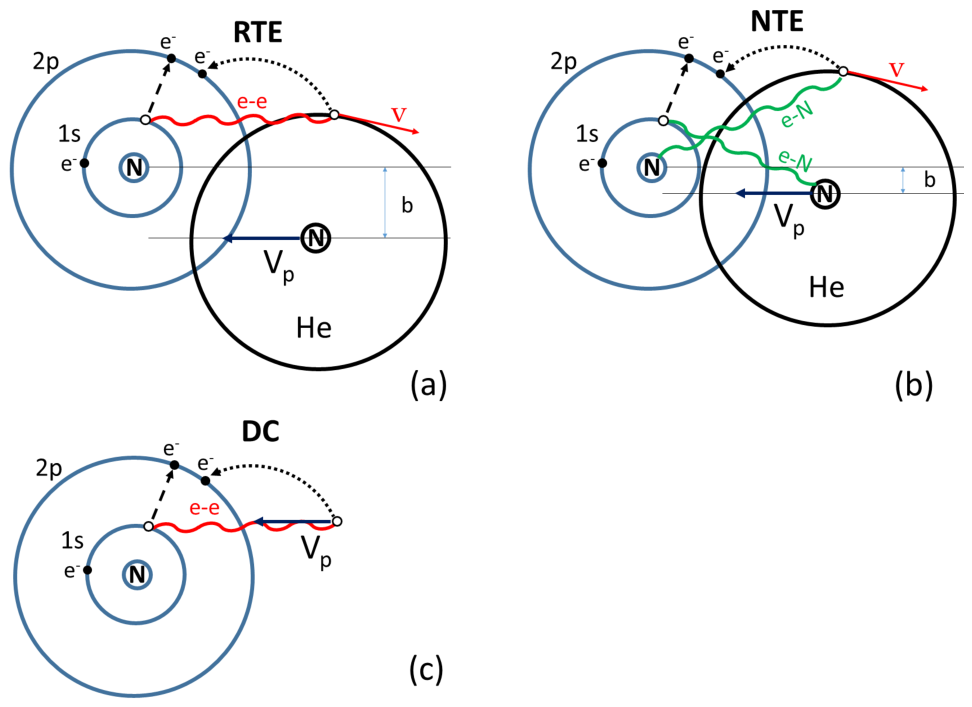
The mechanisms for RTE and NTE differ fundamentally and are shown schematically in Figure 1. The RTE contribution is described to first order by a correlated one-step mechanism mediated by the two-center ( e - e ) interaction [see Figure 1a]. It has been modeled using the IA as a quasifree resonant electron scattering process, analogous to the inverse Auger process [9,10,11,12]. In contrast, NTE arises from a two-step sequence of uncorrelated excitation and transfer events, each driven by independent ( e - N ) interactions [13] [see Figure 1b]. While both TE mechanisms can occur in the same ion–atom collision and contribute coherently to the same final doubly excited projectile state, they have typically been computed separately. This allowed only for the incoherent addition of cross-sections and sparked speculation regarding RTE–NTE interference [13,14,15,16,17,18]. In collisions with light targets such as H2 and He, NTE is significantly suppressed at energies where RTE is dominant and was consequently neglected in early analyses. However, a rigorous and successful (RTE + NTE) treatment has only recently emerged [19].
Following its discovery in 1981 [20], RTE received considerable attention due to its unique and direct connection to dielectronic capture (DC), the analogous resonant ion–electron collision process [21]. In both cases, an impinging electron excites an ion while simultaneously being captured into a bound state. The key difference lies in the nature of the impinging electron: it is free in DC, but bound to the target atom in RTE [see Figure 1a,c] [22]. Both processes lead to the production of short-lived doubly excited states, but only at specific resonant collision energies. Such resonances, while common in electron–ion collisions, are not generally observed in energetic ion–atom collisions since their existence is usually masked by competing ( e - N ) interactions as in NTE [3,7,8]. These resonances are especially pronounced in collisions with ions rather than atoms, due to the greater availability of bound states in the ion–electron continuum compared to the negative ion continuum. Consequently, short-lived resonances appear across a wide range of collision energies and prove highly sensitive to both long-range Coulomb interactions and short-range correlation effects that depend strongly on the ion’s electronic structure and collision dynamics [22,23]. These resonances are stabilized through X-ray (RTEX) or Auger (RTEA) electron emission (also known as the Auger–Meitner effect [24,25,26]), which can be readily measured at accelerator facilities, providing much-needed DC cross-sections—critical for the modeling of plasma charge-state distributions and temperatures, particularly in astrophysical and fusion environments [27,28].
In 1983, Brandt [9] successfully applied the impulse approximation (IA) to describe RTE. For fast collisions where target electrons behave as quasifree (when viewed from the projectile rest frame), RTE was shown to mimic DC. The key difference is that the impinging electron’s kinetic energy is broadened by its orbital motion around the target nucleus. RTE cross-sections could thus be obtained by averaging DC cross-sections over the target’s Compton profile (i.e., the electron momentum distribution along the collision axis). Conversely, DC cross-sections could be indirectly extracted through the IA from RTE measurements. This elegantly simple approach yielded unexpectedly good agreement with the first RTEX measurements, attracting considerable interest by connecting the seemingly disparate fields of ion–atom and ion–electron collisions. It was quickly extended to other processes, including the electron scattering model (ESM) [29], elastic electron scattering off ions [30], resonant inelastic scattering [31], electron excitation [32], electron loss [33,34], and superelastic scattering [35] (see also refs. [36,37] and citations therein). However, success was more modest since these processes also involve ( e - N ) interactions—which the IA does not address—that often contribute significantly in the same collision energy regime, lacking RTE’s clear, unambiguous two-center ( e - e ) interaction signature. The connection between the IA and Born approximation for screening/antiscreening processes was also noted [38].
From 1982 to 1992, TE was extensively studied using He and H2 targets across highly stripped ions ranging from He+ [15] to U90+ [39]. Both the emitted X-rays [40,41,42] and Auger electrons [19,43] from the decay of the TE-formed doubly-excited states were measured, with corresponding cross-sections determined. In particular, KLL state-selective TE measurements were performed, especially for the lowest atomic number Z p projectile ions, using high-resolution Auger projectile spectroscopy [10,11,15,16,44,45,46,47,48], providing the most stringent tests of theory. Both X-ray [41] and Auger [43] spectroscopy measurements tested the validity of the IA and extracted DC cross-sections that were unavailable from direct ion–electron collision experiments at the time [27]. The comprehensive 1992 RTEX [41] and RTEA [43] reviews summarize this remarkably productive era.
Early theoretical treatments of DC cross-sections relied primarily on atomic structure calculations of Auger energies and rates using Hartree–Fock methods [27]. These were followed by more sophisticated electron–ion scattering approaches such as R-matrix [49] and convergent close-coupling methods [50], which coherently account for both long- and short-range interactions. However, experimental KLL DC cross-sections remained scarce in the early 1980s due to insufficient luminosity in crossed-beam or merged-beam setups [22,23]. The advent of high-luminosity electron beams and highly charged ion sources in the late 1980s and early 1990s made direct DC cross-section measurements accessible through merged-beam or crossed-beam experiments [22].
With this capability established, research interest in RTE shifted toward developing rigorous ion–atom collision theories capable of treating TE processes coherently within a uniform approach. These efforts have proven challenging, primarily due to the difficulty of incorporating multiple electrons and both two-center ( e - e ) and ( e - N ) interactions in a unified dynamical treatment [14,51]. Nevertheless, two such dynamical treatments emerged between 1988 and 1997 for two-electron collision systems: (i) the two-electron atomic orbital close-coupling (2eAOCC) method [13], and (ii) the continuum distorted wave four-body (CDW-4B) approach [52,53,54,55]. The 2eAOCC calculations targeted the benchmark He+(1s)+H(1s) system, but the cross-sections for the dominant He(2p2 1D) RTE resonance exceeded measurements for H2 targets (see [56] and Figure 6 in [43]). This approach paved the way for exact nonperturbative TE treatments while refining RTE modeling. The CDW-4B was applied mainly to highly asymmetric systems (e.g., S15++H [52] and references therein), comparing RTE peaks from low-resolution X-ray data, which hindered quantitative interpretation. The NTE peak, occurring at too low an energy, fell outside CDW-4B’s range. Applications to He++He [15,54] and He+(1s)+H(1s) [55] disagreed strongly with experimental and 2eAOCC results [13]. Due to computational limitations and measurement challenges, no further comprehensive coherent treatments followed until recently. Alternative approaches extended the IA to double differential cross-sections (DDCS), enabling uniform treatment of both resonant and nonresonant electron scattering within the ESM [29]. These were supported by state-selective RTEA measurements and R-matrix calculations [12,57].
Advances in computational speed now enable overcoming many of these barriers. In 2022, a nonperturbative TE treatment for 0.5–18 MeV collisions of C4+(1s2) with He was reported, in excellent agreement with measured Auger single differential cross-sections (SDCS) [19] for the production of the C3+(1s2p2 2D) state. This theoretical treatment, (known as 3eAOCC or 3eASCC [58]), considers the dynamics of three active electrons, employing semiclassical close-coupling calculations within a full configuration interaction approach [59]. It enables a coupled, coherent description of target and projectile excitation, ionization, single-electron capture, and TE, therefore going well beyond the methods developed in the past. Collaborative efforts to extend these results to other low- Z p isoelectronic systems are underway.
Following this general introduction, more details about the ion–electron process of DC and its stabilization are first presented in Section 2 and Section 2.2. This is followed by a revised IA treatment connecting ion–electron to ion–atom collisions in Section 3, applied to RTE with new refinements (Section Quadratic IA Treatment) and an exact analytic treatment using screened hydrogenic wavefunctions (Section Exact IA Treatment). The ZAPS technique and advanced capabilities of our hemispherical deflector analyzer (HDA) spectrograph for high-resolution zero-degree Auger spectrometry are then briefly described in Section 4. Representative RTEA results from both older parallel-plate spectrometer measurements and our HDA spectrograph data are systematically compared to the presented revised IA calculations in Section 5. Finally, existing RTEA measurements are comprehensively tabulated and accompanied by a final figure of merit quantifying the significantly improved theory–experiment agreement.
Section 2 is not intended as an exhaustive review of the DC field; rather, it is included to establish the connection with RTE via the IA bridge. Nevertheless, an effort has been made to incorporate some of the most significant references from this area of research.

2. Dielectronic Capture (DC)

For free electrons, capture to an isolated bare ion cannot take place without the emission of photons owing to energy and momentum conservation [60]. However, capture becomes possible for non-bare ions via simultaneous excitation of a bound electron, a process termed dielectronic capture [11] (also known as radiationless capture, RC [9]). Radiative recombination (RR) is also possible, but drops-off fast with increasing electron energy and is therefore usually much less important at energies where DC processes are possible. RR of low-charged ions has been studied in storage rings [61,62].
In DC, a free electron with momentum p = m v and kinetic energy ε = m v 2 / 2 (where m is the mass and v is the velocity of the impinging electron) collides with an N-electron ion, exciting it from level i (binding energy ε i ) while being captured into doubly excited level j (binding energy ε j ) of the resulting ( N + 1 ) -electron ion. The DC cross-section is then given by [63,64]:
σ D C [ i j ] ( ε ) = Ω D C [ i j ] ( ε ) L Γ j ( ε E a ) .
Here, Ω D C [ i j ] ( ε ) denotes the DC collision strength for the i j transition. DC is resonant, peaking at resonance energy E a , the Auger electron energy in the time-reversed j i Auger decay. L Γ j ( ε E a ) is the normalized Lorentzian lineshape of level j (FWHM Γ j ):
L Γ j ( ε E a ) = 1 π Γ j / 2 ( ε E a ) 2 + ( Γ j / 2 ) 2 .
For doubly excited j-levels, Γ j | ε E a | except near resonance ( ε E a ), yielding a very narrow profile often approximated by a Dirac delta function [63,65]:
L Γ j ( ε E a ) δ ε E a ,
leading to:
σ D C [ i j ] ( ε ) = Ω D C [ i j ] ( ε ) δ ε E a .

2.1. The DC Collision Strength Ω D C

The collision strength Ω D C [ i j ] ( ε ) in Equation (1) is given by [63]:
Ω D C ( ε ) Ω D C [ i j ] ( ε ) = π 2 2 a 0 2 ε 0 g j g i A a [ j i ] ε ,
where a 0 is the Bohr radius, and ε 0 is the atomic unit of energy ( 27.211386 eV). Here, g i = ( 2 L i + 1 ) ( 2 S i + 1 ) and g j = ( 2 L j + 1 ) ( 2 S j + 1 ) are the L S -coupling degeneracies; A a [ j i ] is the ( j i ) Auger rate with transition energy E a = ε i ε j . At resonance ( E a in eV and A a in s−1), Ω D C is given by:
Ω D C ( ε = E a ) [ cm 2 eV ] = 2.4751 × 10 30 ( 2 L j + 1 ) ( 2 S j + 1 ) ( 2 L i + 1 ) ( 2 S i + 1 ) A a [ j i ] E a [ j i ] .

2.2. DC Level Relaxation by Photon or Auger Emission

The doubly excited DC state j stabilizes via photon or Auger emission. Photon decay to a final state f of the ( N + 1 ) -electron ion ( i j f ) yields dielectronic recombination (DR). Alternatively, Auger decay returning to an N-electron final state f ( i j f , where f = i or f i ) yields resonant excitation (RE) [10,66]:
σ D R [ i j f ] ( ε ) = σ D C [ i j ] ( ε ) ω [ j f ] ,
σ R E [ i j f ] ( ε ) = σ D C [ i j ] ( ε ) ξ [ j f ] ,
with the fluorescent yield defined as:
ω [ j f ] A r [ j f ] ( f A a [ j f ] + f A r [ j f ] )
and the Auger yield defined as:
ξ [ j f ] A a [ j f ] ( f A a [ j f ] + f A r [ j f ] ) .
DR cross-sections for highly charged ions (H-like [64,67,68], He-like [69,70,71], Li-like [72,73,74,75,76,77]) and Be-like [78] have been accurately measured in storage ring electron coolers via merged beams, finely scanning the electron energy ε while detecting the recombined ions. Atomic structure models continue to advance across diverse applications. Recent efforts include calculating partial and total recombination rate coefficients for the entire tungsten isonuclear sequence for collisional–radiative fusion modeling at the International Thermonuclear Experimental Reactor (ITER) [79], investigating capture into high-n Rydberg shells relevant to low-temperature plasma dynamics [80], and calculating DR in low-charge ions for kilonovae and nonlocal thermodynamic equilibrium (non-LTE) plasmas [81].
For Auger emission at angles ( θ e , ϕ e ) relative to the electron beam, the RE collision strength and SDCS are [82]:
Ω R E [ i j f ] ( ε ) = Ω D C [ i j ] ( ε ) ξ [ j f ] ,
d σ R E d Ω e [ i j f ] ( ε , θ e , ϕ e ) = σ R E [ i j f ] ( ε ) Y L , M L = 0 ( θ e , ϕ e ) 2 ,
where Y L M is the spherical harmonic. Axial symmetry populates only M L = 0 , favoring forward/backward ( θ e = 0 , 180 ) emission along the beam (z-axis), where | Y L , M L = 0 ( 0 ° ) | 2 = | Y L , M L = 0 ( 180 ° ) | 2 = ( 2 L + 1 ) / ( 4 π ) . When i = f , RE equates to resonant elastic electron scattering.
For X-ray emissions at angles ( θ x , ϕ x ) relative to the electron beam, the DR collision strength and SDCS are given by (see ref. [83] and references therein):
Ω D R [ i j f ] ( ε ) = Ω D C [ i j ] ( ε ) ω [ j f ] ,
d σ D R d Ω x [ i j f ] ( ε , θ x , ϕ x ) = σ D R [ i j f ] ( ε ) 4 π 1 + β 2 [ i j f ] P 2 ( cos θ x ) ,
where P 2 ( cos θ x ) is the second-order Legendre polynomial. Equation (14) is valid for dipole ( E 1 ) radiation with β 2 ( ε ) given in ref. [83]. An improved semi-empirical Z p -dependence of Ω D R has also been presented in [83], which includes higher-order relativistic corrections especially relevant for heavy, highly charged ions typically studied in storage rings.

2.3. Dielectronic Recombination Rate α D R ( T )

The DR rate α D R at plasma temperature T is [63,84]:
α D R [ i j f ] ( T ) 0 σ D R [ i j f ] ( v ) v g ( v , T ) d v ,
with Maxwell–Boltzmann distribution [63]:
v g ( v , T ) d v = 2 m 3 π ( k B T ) 3 v 2 exp m v 2 2 k B T v d v ,
where k B is the Boltzmann constant and the product k B T is in eV. Substituting Equation (7) for σ D R , Equation (1) for σ D C and converting to energy ε yields:
α D R [ i j f ] ( T ) = 4 ω [ j f ] ( k B T ) 3 / 2 2 π m 0 Ω D C [ i j ] ( ε ) L Γ j ( ε E a [ j i ] ) ε exp ε k B T d ε .
Using the delta-function approximation (Equation (3)) simplifies to:
α D R [ i j f ] ( T ) = 4 ω [ j f ] ( k B T ) 3 / 2 2 π m Ω D C ( ε = E a [ j i ] ) E a [ j i ] exp E a [ j i ] k B T .
Using Equation (5) at ε = E a then gives α D R [63]:
α D R [ i j f ] ( T ) [ cm 3 / s ] = 1.6564 × 10 22 ( k B T ) 3 / 2 ( 2 L j + 1 ) ( 2 S j + 1 ) ( 2 L i + 1 ) ( 2 S i + 1 ) A a [ j i ] ω [ j f ] exp E a [ j i ] k B T .
Thus, DC cross-sections and DR rates require only atomic structure calculations for A a , E a , and the fluorescence yield ω . Although the importance of DR in coronal plasmas was recognized as early as the 1960s [85], cross-section data relied entirely on theory until the first measurements in the early 1980s [86,87,88,89,90] using crossed-beam experiments. The development of electron beam ion sources (EBIS) [91,92] and traps (EBIT) [93], alongside electron cooled ion storage rings (SR), subsequently enabled high-resolution merged-beam experiments [69,94]. Early insights into DC came indirectly from RTE in ion–atom collisions; these processes are linked via the IA, which treats bound target electrons as quasifree, allowing for the extraction of DC, RE, and DR cross-sections. Comprehensive reviews of electron–ion processes include refs. [22,23], with refs. [94,95,96] focusing specifically on heavy-ion SRs.

3. The Impulse Approximation (IA)

3.1. Quasi-Free Electron Scattering

A bound electron enters the collision with a normalized momentum distribution F ( p ) , determined by its orbital momentum p = m v around the target. In the ion’s rest frame (denoted by primes), the target electron moves toward the ion with velocity V p , yielding a net impinging velocity v = V p + v . For fast collisions, the IA validity criterion:
η V p / v 1
ensures that the impinging electron’s distribution F ( p ) is centered around V p .
The IA assumes that free electron–ion impact cross-sections relate to their bound (or quasifree) analogs via [60,97]:
σ q u a s i f r e e ( V p ) = + d p σ f r e e ( ϵ ) F ( p ) δ ( E f E i ) ,
where the delta function δ ( E f E i ) enforces energy conservation between the total initial energy E i and final energy E f of the interacting target-electron–ion system [97] and depend on the process at hand. The impinging momentum p and kinetic energy ϵ of the quasifree electron are:
p = m V p + p
ϵ = p 2 2 m = 1 2 m V p 2 + p 2 2 m + V p · p .
Aligning the projectile velocity along the z-axis ( V p = V p z ^ ), Equation (23) becomes:
ϵ = ϵ ( V p , p , p z ) = 1 2 m V p 2 + p x 2 + p y 2 + p z 2 2 m + V p p z
with
p = p ( V p , p , p z ) = 2 m ϵ ( V p , p , p z ) .
Both p and ϵ depend on the orbital momentum p (or its components) and projectile velocity V p . The use of the free-electron cross-section σ f r e e in Equation (21) assumes the projectile states remain undistorted by the target nucleus or other target electrons. This is justified for Z t Z p [60], where Z p and Z t are the atomic numbers of the projectile and target, respectively.
The ion rest-frame momentum distribution F ( p ) combines the fixed momentum m V p from relative projectile-target motion with the lab-frame orbital momentum p around the target, distributed as | Φ ( p ) | 2 . It centers on m V p since the impinging electron averages this momentum toward the stationary ion:
F ( p ) d p = Φ ( p ) 2 d p with Φ ( p ) 2 d p = 1 .
For short interactions, the target electron remains frozen, so
Φ ( p ) Φ i ( p ) ,
where Φ i ( p ) is the initial target momentum wave function. Substituting in Equation (21) yields:
σ q u a s i f r e e ( V p ) = + d p σ f r e e ( ϵ ) Φ i ( p ) 2 δ ( E f E i ) .
Equation (28), with ϵ from Equation (24), forms the IA’s core equation. It assumes the initial momentum distribution | Φ i ( p ) | 2 stays undisturbed and projectile resonance states experience negligible distortion by the approaching target. This formulation first appeared in 1970 for Compton scattering of photons off target electrons [98,99]. Kleber and Jakubassa [97] applied it in 1975 to radiative electron capture (REC) using the known radiative recombination (RR) cross-section. In 1982, Tanis et al. [5] observed a broad peak in the cross-section for electron capture with projectile excitation (S13+(1s22s) + Ar), attributed to RTE. Brandt [9] explained it via the IA, linking RTE to the DC cross-section and predicting the resonance’s V p dependence and peak position.
The following section details the IA RTE treatment, building on Brandt’s foundational work [9] and subsequent refinements by Lee et al. [30]. We introduce a critical correction for low Z p 9 ions that largely resolves the long-standing divergence between theory and experiment for low- Z p ions [43]. Furthermore, we demonstrate an exact analytical treatment of the IA, providing deeper insight into the validity of previous approximations.

3.2. IA RTE

3.2.1. Total Cross-Sections

Brandt [9] extended the IA from radiative capture [97] to RTE by applying Equation (28) with the corresponding DC cross-section:
σ R T E [ i j ] ( V p ) = + d p σ D C [ i j ] ( ϵ ) Φ i ( p ) 2 δ ( E f E i ) .
For the RTE process the total initial and final energies are:
E i = ε i P ε i T + ϵ
E f = ε f P ε f T .
Here, ϵ is the impinging target electron kinetic energy given by Equation (24), while ε i T , ε f T denote initial and final target and ε i P , ε f P projectile binding energies, respectively (all negative quantities). Defining E I ε i T ε f T (target ionization energy) and E a = ε i P ε f P (Auger energy for j i decay) yields:
E f E i = E a + E I ϵ .
At resonance, E f = E i so the impinging resonance electron energy is ϵ = ϵ R where ϵ R is:
ϵ R = E a + E I ,
with E I given in Table 1 for H2 and He, the targets of interest here.
Thus, Equation (29) simplifies to:
σ R T E ( V p ) = + d p σ D C ( ϵ ) Φ i ( p ) 2 δ ( ϵ ϵ R ) ,
omitting [ i j ] labels for brevity.
Quadratic IA Treatment
The three-dimensional integral over d p simplifies by assuming only the p z component contributes significantly [Equation (24)]:
ϵ = ϵ ( V p , p z ) 1 2 m V p 2 + p z 2 2 m + V p p z ( quadratic IA ) .
This formulation improves upon Brandt’s original linear approximation by retaining both linear and quadratic p z terms. Further, using the target Compton profile definition (see Appendix A):
J ( p z ) d p x d p y Φ i ( p ) 2 ,
the RTE cross-section then becomes:
σ R T E ( V p ) = d p z σ D C ( ϵ ( V p , p z ) ) J ( p z ) δ ( ϵ ( V p , p z ) ϵ R ) ,
where J ( p z ) has been normalized to 2 for two-equivalent-electron targets (see Appendix A). The resonance condition is provided by the delta function, where the resonance energy ϵ R was already defined in Equation (33). To evaluate the integral, we transform the delta function using δ ( ϵ ϵ R ) = δ ( p z p R ) / | ϵ / p z | p R . For the quadratic case, setting ϵ ( V p , p R quad ) = ϵ R leads to the derivative:
ϵ p z p R quad = p R quad m + V p = 2 ϵ R m .
Thus, performing the integration over the transformed delta-function in Equation (37) and using the definition of σ D C in terms of the collision strength Ω D C (Equation (1)) we obtain:
σ R T E ( V p ) = Ω D C ( ϵ ( V p , p R quad ) ) J ( p R quad ( V p ) ) 2 ϵ R m ( quadratic IA ) ,
where p R quad is defined through Equation (38) with Ω D C [ i j ] ( ε ) from Equation (5) evaluated for ε = ϵ R :
Ω D C ( ϵ R ) = Ω D C ( ε = E a ) E a E a + E I .
Substituting in Equation (39) yields:
σ R T E ( V p ) = Ω D C ( E a ) E a E a + E I J ( p R quad ( V p ) ) 2 ϵ R m ( r e v i s e d quadratic IA ) ,   (41)
σ R T E ( V p ) = Ω D C ( E a ) J ( p R quad ( V p ) ) 2 ϵ R m ( o l d e r quadratic IA ) ,   (42)
p R quad ( V p ) = m V p + 2 m ϵ R ( quadratic IA ) .   (43)
This result introduces a target ionization correction factor, E a / ( E a + E I ) , which was absent in prior treatments [11,43,82]. Results including this correction are hereafter termed “revised.” While negligible for Z p > 10 , this correction is substantial for lighter ions. For example, in He + + He (2p2 1D), it reduces σ R T E by 41% (factor of 0.589); for C 4 + + He (1s2p2 2D), it reduces it by 10% (factor of 0.908).
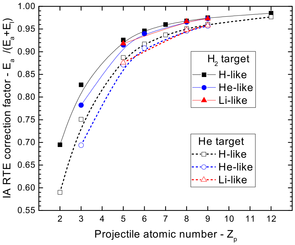
This modification effectively resolves the long-standing systematic theory-experiment discrepancy observed as Z p decreases, significantly improving agreement for Z p 9 [43] without altering the V p dependence governed by J ( p R ( V p ) ) . Correction factor values are provided in Table 2, Table 3 and Table 4 and plotted in Figure 2 as a function of Z p .
Linear IA Treatment
Neglecting the p z 2 / 2 m term in Equation (35) yields the linear form:
ϵ 1 2 m V p 2 + V p p z ( linear IA ) .
Working as previously, at the resonance ( ϵ = ϵ R ), the derivative simplifies to | ϵ / p z | = V p , leading to:
σ R T E ( V p ) = Ω D C ( E a ) E a E a + E I J ( p R lin ( V p ) ) V p ( r e v i s e d linear IA ) ,  (45)
σ R T E ( V p ) = Ω D C ( E a ) J ( p R lin ( V p ) ) V p ( o l d e r linear IA ) ,  (46)
p R lin ( V p ) = ϵ R V p 1 2 m V p ( linear IA ) .  (47)
Exact IA Treatment
The IA can also be evaluated exactly by utilizing the explicit momentum distribution | Φ i ( p ) | 2 (e.g., hydrogenic) alongside the σ D C from Equation (1). This exact IA approach, presented here, provides a rigorous benchmark that appears to have been overlooked in previous literature.
In spherical coordinates, Equation (34) is expressed as:
σ R T E ( V p ) = 0 p 2 d p 0 π sin θ d θ 0 2 π d ϕ σ D C ( ϵ ) | Φ i ( p ) | 2 δ ( ϵ ϵ R ) . ( exact IA )
We now use the exact expression for the electron energy in the projectile frame:
ϵ ( V p , z , p ) = 1 2 m V p 2 + p 2 2 m + V p z p ( exact IA ) ,
with z = cos θ . Assuming an isotropic distribution | Φ i ( p ) | 2 = | Φ i ( p ) | 2 / ( 4 π ) , the ϕ integration yields:
σ R T E ( V p ) = 1 2 0 p 2 d p 1 1 d z σ D C ( ϵ ( V p , z , p ) ) | Φ i ( p ) | 2 δ ( ϵ ( V p , z , p ) ϵ R ) . ( exact IA )
Substituting the Lorentzian form of σ D C from Equation (1), we obtain:
σ R T E ( V p ) = 1 2 Ω D C ( E a ) 0 p 2 d p 1 1 d z E a ϵ ( V p , z , p ) L Γ j ( ϵ ( V p , z , p ) ϵ R ) | Φ i ( p ) | 2 . ( exact IA )
Modeling the targets H2 and He by screened hydrogenic ground states, we set | Φ i ( p ) | 2 = 2 | F 10 ( p ) | 2 , where the factor of 2 accounts for the two equivalent electrons in the real targets (see Appendix A). We use [103]:
| F 10 ( p ) | 2 = 2 5 π ( Z t p 0 ) 5 [ p 2 + ( Z t p 0 ) 2 ] 4 ,
where p 0 is the atomic unit of momentum. The screened hydrogenic charges Z t are given in Table 1 and are chosen to match measured Compton profiles [100] (see Appendix A). Equation (51) can then be written in analogy with the approximate IA cross-sections as:
σ R T E ( V p ) = Ω D C ( E a ) E a E a + E I I 10 ( V p , ϵ R ) , ( exact IA )
where I 10 is the double integral:
I 10 ( V p , ϵ R ) ϵ R 0 | F 10 ( p ) | 2 1 1 d z L Γ j ( ϵ ( V p , z , p ) ϵ R ) ϵ ( V p , z , p ) p 2 d p .
While the integral I 10 can be evaluated numerically, an analytical solution is possible by replacing the Lorentzian with a delta function. This approximation is highly accurate since the resonance width Γ j is much smaller than the energy ϵ R . The resulting analytical derivation is detailed in Appendix B. Using the analytic result for I 10 from Equation (A6) we obtain:
σ R T E ( V p ) = Ω D C ( E a ) E a E a + E I 16 3 π Z t p 0 p ˜ 2 + 1 3 p ˜ + 2 + 1 3 V p
( exact IA ) ,  (55)
p ˜ ± = m V p ± 2 m ϵ R Z t p 0
( exact IA )  (56)

3.2.2. Single Differential Cross-Sections (SDCS)

Most RTE measurements detect emitted X-rays or Auger electrons at specific angles ( θ , ϕ ) relative to the ion beam, yielding SDCS. In the rest frame, the RTEA SDCS for an i j f transition in LS-coupling (assuming S i = S f = 0 ) is given by [82]:
d σ R T E A d Ω e ( V p , θ e ) = ξ σ R T E ( V p ) ( 2 L j + 1 ) 4 π [ P L j ( cos θ e ) ] 2 ,
where ξ is the Auger yield for the decay to the final state L f S f and P L j ( x ) is the Legendre polynomial of order L j . While there have been some measurements of RTEA SDCS at non-zero angles verifying Equation (57) [16,17,104,105,106], most subsequent RTEA studies have focused on zero-degree measurements, which are of primary concern here. For laboratory observations at θ e = 0 , the corresponding rest-frame angle is θ e = 0 or 180 [107], leading to:
d σ R T E A d Ω e ( V p , θ e = 0 ) = ξ σ R T E ( V p ) ( 2 L j + 1 ) 4 π .
These general SDCS expressions apply to all IA models, where σ R T E ( V p ) represents the specific RTE cross-section for the corresponding model (Equations (41), (45), or (55)). For the zero-degree observations of interest here, applying Equation (58) and converting to E p instead of V p yields in each case:
For the Quadratic IA
d σ R T E A quad ( E p , 0 ) d Ω e [ cm 2 / sr ] = d σ R E ( 0 ) d Ω e [ cm 2 / sr ] E a E a + E I J ( p R ( E p ) ) [ a . u . ] 2 ϵ R [ a . u . ] ,
( revised )  (59)
p R quad ( E p ) [ a . u . ] = 6.3498 E p [ MeV / u ] + 0.4031 ϵ R [ a . u . ] .
 (60)
For the Linear IA
d σ R T E A lin ( E p , 0 ) d Ω e [ cm 2 / sr ] = d σ R E ( 0 ) d Ω e [ cm 2 / sr ] E a E a + E I J ( p R lin ( E p ) ) [ a . u . ] V p [ a . u . ] ,
( revised )  (61)
p R lin ( E p ) [ a . u . ] = 0.1575 ϵ R [ a . u . ] E p [ MeV / u ] 3.1749 E p [ MeV / u ] .
 (62)
For the Exact IA
d σ R T E A exact ( E p , 0 ) d Ω e [ cm 2 / sr ] = d σ R E ( 0 ) d Ω e [ cm 2 / sr ] E a E a + E I ε 0 I 10 ( V p , ϵ R ) = d σ R E ( 0 ) d Ω e [ cm 2 / sr ] E a E a + E I
 (63)
· 16 3 π Z t p ˜ [ a . u . ] 2 + 1 3 p ˜ + [ a . u . ] 2 + 1 3 V p [ a . u . ] ,
( exact )  (64)
p ˜ ± [ a . u ] = V p [ a . u . ] ± 2 ϵ R [ a . u . ] Z t .
 (65)
In the above expressions, we have utilized d σ R E ( 0 ) d Ω e as a shorthand notation defined by:
d σ R E ( 0 ) d Ω e [ cm 2 / sr ] Ω R E ε 0 ( 2 L j + 1 ) 4 π = 7.1677 × 10 33 ( 2 L j + 1 ) 2 ( 2 S j + 1 ) ( 2 L i + 1 ) ( 2 S i + 1 ) A a [ j i ] E a [ j i ] ,
where Ω R E is given by Equations (6) and (11), and the numerical constant incorporates the 1 / ( 4 π ε 0 ) factor. The projectile velocity V p [a.u.] as a function of E p [MeV/u] is:
V p [ a . u . ] = 2 m M p 10 6 E p ε 0 6.3498 E p [ MeV / u ] ,
where M p is the mass of the projectile. Notably, d σ R E ( 0 ) d Ω e depends on ( 2 L j + 1 ) 2 , explaining why high- L j states, such as D-states ( L j = 2 ), dominate RTEA measurements. While the uncorrected quadratic form is identical to Equation (18) of ref. [43], these approximate treatments are ultimately superseded by the exact analytic expression of Equation (64).
We note that since V p appears in the denominator of the linear and exact IA expressions (Equations (61) and (64)), analytically determining the SDCS maximum as a function of V p is difficult, requiring a numerical solution. However, the quadratic model (Equation (59)) lacks this V p dependence, allowing the SDCS to reach a well-defined maximum exactly at resonance ( p R = 0 ) where J ( 0 ) peaks. Thus, for the revised quadratic IA, we may write for practical convenience:
d σ R T E A quad ( E p , 0 ) d Ω e [ cm 2 / sr ] = d σ R T E A max ( 0 ) d Ω e [ cm 2 / sr ] J ( p R quad ) [ a . u . ] J ( 0 ) [ a . u . ] ,
with
d σ R T E A max ( 0 ) d Ω e [ cm 2 / sr ] = d σ R E ( 0 ) d Ω e [ cm 2 / sr ] E a E a + E I J ( 0 ) [ a . u . ] 2 ϵ R [ a . u . ]
( r e v i s e d quadratic IA ) ,  (69)
V p max 2 ϵ R m
( quadratic IA ) ,  (70)
E p max 1 2 M p V p max 2 = M p m ϵ R
( quadratic IA ) ,  (71)
η max V p max v = ϵ R K I
( quadratic IA ) ,  (72)
where V p max and E p max are the projectile velocity and kinetic energy at the resonance maximum, and J ( 0 ) is given in Table 1 and Appendix A. Here, d σ R T E A max ( 0 ) d Ω e depends on the RE collision strength Ω R E and remains constant across different IA variants. Consequently, the SDCS in Equation (68) is directly proportional to the target Compton profile J ( p R ( E p ) ) . This relationship, confirmed by experimental data, validates the IA’s assumption that fast collisions preserve the initial target electron momentum distribution.
The figures in Section 5 compare experimental zero-degree SDCS with the three IA models: the exact analytic IA (green, Equation (64)), the revised quadratic IA (blue, Equation (59)), and the older quadratic baseline (black, Equation (59) without the E a / ( E a + E I ) factor). The IA validity criterion (Equation (20)) is quantified at the resonance by η max , where K I = m v 2 / 2 is the target electron kinetic energy given in Table 1. Values for η max , E p max , and d σ R T E A max ( 0 ) / d Ω e are listed in Table 2, Table 3 and Table 4 and indicated in the figures.

3.2.3. Double Differential Cross-Sections (DDCSs) and the Electron Scattering Model (ESM)

The ESM [29,30] has shown that the IA can also be applied directly to DDCS [12] with great success. According to the ESM, the quasifree DDCS can be related to the free electron SDCS by:
d 2 σ ( ε , θ e , ϕ e ) d Ω e d ε quasifree = d σ ( ε , θ e , ϕ e ) d Ω e free J ( p z ) 2 ( ε + E I ) m ,
where, in the quadratic IA instead of Equations (35) and (43), we have:
ε 1 2 m V p 2 + p z 2 2 m + V p p z
and therefore
p z = m V p + 2 m ε .
Substituting the RE SDCS [Equation (12)] for the free electron SDCS and integrating over ε recovers the RTEA SDCS (Equation (57)):
d σ ( ε , θ e , ϕ e ) d Ω e quasifree = d 2 σ ( ε , θ e , ϕ e ) d Ω e d ε quasifree d ε = Ω R E ( E a ) ( 2 L j + 1 ) 4 π [ P L j ( cos θ e ) ] 2 E a E a + E I J ( p R quad ) ( V p ) 2 ϵ R m ( r e v i s e d quadratic IA ) ,
with p R quad from Equation (43). Energy conservation shifts the free-electron δ ( ε E a ) [Equation (4)] to quasifree δ ( ε ϵ R ) , introducing again the correction factor E a / ( E a + E I ) .
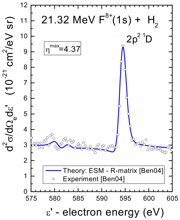
Substituting in Equation (73) the non-resonant elastic ion–electron scattering SDCS yields the binary encounter electron (BEe) peak. Its excellent agreement with the experiment for bare ions [30] has established it as the preferred standard for the in situ absolute calibration of electron spectrometer efficiencies [107]. Bhalla [29] unified the resonant (RTEA) and non-resonant elastic electron scattering (BEe) for H-like ions + He, thus also including BEe-RTEA interference. R-matrix-enhanced free-electron SDCS further improved results for low- Z p H-like [12,57,108], boron He-like [12], resonant inelastic [31,109], and even superelastic scattering [35]. An example of the IA ESM–R-matrix agreement at the DDCS level is shown in Section 5 for 21 MeV F8++H2 collisions.
A detailed discussion of the ESM is beyond the scope of this review, as it primarily involves electron–ion scattering theory and computational methods (e.g., R-matrix). Interested readers are referred to the previously cited literature for further details.
Table 2. Results for the 2p2 1D state production via RTEA in H-like [ X Z p 1 ( 1 s ) ] ion collisions with He and H2 targets (references provided in the last column). Theoretical RE collision strengths, Ω R E , are calculated using tabulated Auger rates ( A a ), energies ( E a ), and yields ( ξ ). Listed are the zero-degree IA RTEA maximum SDCS d σ R T E A max ( 0 ) / d Ω e , the resonance projectile energy E p max , and the IA validity criterion η max = V p max / v . Comparison with experimental maximum SDCS d σ Exp max ( 0 ) / d Ω e yields the ratio r (Equation (77)) and the extracted strength Ω R E Exp = r Ω R E (Equation (78)). For cases where SDCS values were unavailable, Ω R E Exp is taken directly from the cited references and shown in parentheses; these are then used to compute the corresponding r values (also in parentheses) using our calculated Ω R E from column 9. Blank entries denote repeated values from the row above, while dashes (-) indicate unavailable SDCS data. Results for B4++H2 and He+ +H2 are discussed and shown in the figures of Section 5.
TheoryExperiment
Collision System Z p A a  a E a  a ξ  a E a E a + E I η max E p max Ω RE d σ RTEA max d Ω e d σ Exp max d Ω e  b r  c r Ω RE  d
( s 1 ) (eV) (MeV/u) (cm2eV) (cm2/sr) (cm2/sr) (cm2eV)
( × 10 14 ) ( × 10 19 ) ( × 10 20 ) ( × 10 20 ) ( × 10 19 )
(Equation (72)) (Equation (71)) (Equations (6) and (11)) (Equation (69)) (Equation (77)) (Equation (78)) Refs.
X Z p 1 ( 1 s ) + T X Z p 2 ( 2 p 2   D 1 ) X Z p 1 ( 1 s ) + e A
3He++He21.0935.33 e1.0000.5901.230.109191.68.380.480.05711[15]
   +H2 0.6951.260.093 15.513.570.23044.7[56]
7Li2++He31.60 f74.32 g0.9990.7511.580.180133.45.79---[110]
11B4++H252.86193.26 h0.9960.9262.560.38191.174.865.301.1099.4[111]
(90.41) -(0.845)(77) i[12]
(84) -(0.879)(80.1)[112]
12C5++He62.52273.30 h0.9940.9172.750.54356.731.731.801.0459.9[48]
   +H2 0.9463.010.526 2.622.500.9554.0[48]
(66.5 i) -(1.16)(66) i[57]
14N6++H272.68366.9 j0.9910.9603.460.69744.751.82---This work l
(51.0) i -(1.16)(52) i[57]
16O7++H283.12474.2 j0.9860.9683.910.89340.141.46---This work l
(40.1) i -(1.05)(42) i[57]
19F8++H292.90595.0 j0.9770.9754.371.11329.460.9650.880.90726.7[45]
(32.31) -(1.12)(33)[12]
(35.00) -(1.19)(36) i[57]
(32.3) -(1.09)(32.2)[112]
24Mg11++H2123.081038.6 k0.9270.9855.741.92217.000.428---This work l
(19.1) -(1.31)(22.2)[112]
a  A a , E a and ξ from various sources as indicated. A a are mostly from the MZ code based on the Z-expansion method with relativistic corrections [113] except for helium [114] and boron [12]. For carbon, the truncated-diagonalization method [115] gives the same results. b Absolute experimental error reported ∼20–30% in most refs. c Values of r are also shown in the last figure of Section 5 as a function of projectile atomic number Z p with an overall uncertainty of 30 %. d Values in parentheses as reported in the corresponding reference unless otherwise indicated. e From ref. [116]; f complex rotation method [117]; g measured by Rodbro et al. [110]; h reported in ref. [12]; i reported in ref. [112]; j reported in ref. [112], originally from ref. [118]; k reported in ref. [112] as T.W. Gorczyca (private communication); l this work refers only to the IA RTE calculations. No RTEA measurements exist for this collision system.
Table 3. As in Table 2, but for the production of the 1s2p2 2D state in collisions of ground-state He-like [ X ( Z p 2 ) + ( 1 s 2 ) ] ions. Results for carbon, fluorine and boron are discussed and shown in the figures of Section 5.
TheoryExperiment
Collision System Z p A a  a E a  a ξ  a E a E a + E I η max E p max Ω RE d σ RTEA max d Ω e d σ Exp max d Ω e  b r  c r Ω RE  d
( s 1 ) (eV) (MeV/u) (cm2eV) (cm2/sr) (cm2/sr) (cm2eV)
( × 10 14 ) ( × 10 19 ) ( × 10 20 ) ( × 10 20 ) ( × 10 19 )
(Equation (72)) (Equation (71)) (Equations (6) and (11)) (Equation (69)) (Equation (77)) (Equation (78)) Refs
X Z p 2 ( 1 s 2 ) + T X Z p 3 ( 1 s 2 p 2 D 2 ) X Z p 2 ( 1 s 2 ) + e A
7Li++He30.169 e55.67 f1.0000.6941.430.14674.93.33---[119]
11B3++H250.633 e166.50 f1.0000.9152.390.33294.15.306.321.1989.1[12]
12C4++He60.756242.15 g0.9990.9082.590.48577.482.4752.451.0077.51[19]
16O6++He80.988434.310.9870.9463.410.83756.301.4281.80 h1.2872.1-
19F7++He91.07551.200.9790.9573.821.05047.011.0760.960.9544.7[120]
   +H2 0.9734.211.033 1.5951.340.8439.5[120]
a  A a , E a and ξ from various sources as indicated. A a are mostly from the MZ code based on the Z-expansion method with relativistic corrections [113] except for helium [114] and boron [12]. For carbon, the truncated-diagonalization method [115] gives the same results. b Absolute experimental error reported ~20–30% in most refs. c Values of r are also shown in the last figure of Section 5 as a function of projectile atomic number Zp with an overall uncertainty of ≲30%. d Values in parentheses as reported in the corresponding reference unless otherwise indicated. e B-spline method [121]; f measured by Rodbro et al. [110]; g measured by Rodbro et al. [110]; recalibrated by Bruch et al. [122]; h to be published.
Table 4. As in Table 2, but for the production of the 1s2s2p2 3D and 1D states in collisions of Li-like [ X ( Z p 3 ) + ( 1 s 2 2 s ) ] ions.
TheoryExperiment
Collision System Z p A a  a E a  a ξ  a E a E a + E I η max E p max Ω RE d σ RTEA max d Ω e d σ Exp max d Ω e  b r  c r Ω RE  d
( s 1 ) (eV) (MeV/u) (cm2eV) (cm2/sr) (cm2/sr) (cm2eV)
( × 10 14 ) ( × 10 19 ) ( × 10 20 ) ( × 10 20 ) ( × 10 19 )
(Equation (72)) (Equation (71)) (Equations (6) and (11)) (Equation (69)) (Equation (77)) (Equation (78)) Refs
X Z p 3 ( 1 s 2 2 s ) + T X Z p 4 ( 1 s 2 s 2 p 2 D 3 ) X Z p 3 ( 1 s 2 2 s ) + e A
11B2++H250.490173.600.8910.9182.430.34546.62.582.350.9142.4[111]
16O5++He81.05448.680.8790.9483.460.86138.20.9550.260 e0.27210.4[10]
   +H2 0.9673.810.845 1.4220.8750.61523.5[44]
19F6++He91.11567.680.8780.9583.871.08031.80.7180.34 e0.47415.1[11]
   +H2 0.9734.271.063 0.52 f0.48915.6[11]
   +H2 0.78 g0.73323.3[44]
X Z p 3 ( 1 s 2 2 s ) + T X Z p 4 ( 1 s 2 s 2 p 2 D 1 ) X Z p 3 ( 1 s 2 2 s ) + e A
11B2++H250.387176.830.3980.9192.450.3515.390.2970.602.010.9[111]
16O5++He80.89455.350.4600.9493.490.8705.550.1380.056 e0.4062.25[10]
   +H2 0.9673.840.854 0.2050.200.9765.42[44]
19F6++He91.10575.550.4690.9593.901.0955.530.1240.088 e0.7103.92[11]
   +H2 0.9744.301.078 0.1840.20 g1.026.01[44]
a  A a , E a , ξ for the 3D state from ref. [123], while for the 1D state from ref. [11] for oxygen and fluorine and from [124] for boron and carbon. b Absolute experimental error reported around 20–25% and 30% for refs. [10,11]. c Values of r are also shown in 15 the last figure of Section 5 as a function of projectile atomic number Z p with an overall uncertainty of 30 %. d Values in parentheses as reported in the corresponding reference unless otherwise indicated. e After subtraction of NTEA contributions. Collisions with H2 targets have minimal NTEA not subtracted. f Absolute electron detector efficiency based on normalization to target Ne K-Auger cross-sections from 3 MeV collisions with protons. g Revised absolute electron detector efficiency based on normalization to BEe DDCS by bare ions.

4. Zero-Degree Auger Projectile Spectroscopy (ZAPS)

ZAPS detects electrons emitted from fast ionic projectiles at θ e = 0 relative to the beam direction, where optimal kinematic conditions maximize energy resolution. This enables LS-resolved (state-selective) Auger spectra, providing a powerful probe of fast ion–atom collision dynamics and stringent tests of theory. ZAPS favors low- Z p projectiles ( Z p < 30 ) due to high Auger yields (>90% for Z p < 10 ), surpassing X-ray fluorescence. The technique, introduced in the early 1980s [125], is reviewed in refs. [107,126].
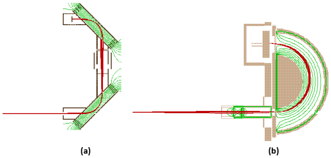
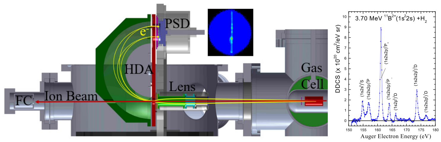
Early ZAPS used two 45° parallel-plate analyzers (2PPA) in series (tandem) [Figure 3a], but since the 2000s, a single-stage paracentric [127,128] hemispherical deflector analyzer (HDA) with injection lens and 2D position sensitive detector (2D PSD) has been used in our group [Figure 3b]. Such an HDA spectrograph can record a ∼20% energy window simultaneously, avoiding 2PPA voltage scanning, thus boosting detection efficiency by over two orders of magnitude [129]. This HDA uses an unusual virtual entry aperture for the uninhibited passage of the ion beam through the spectrometer, while optimized [130,131] for high transmission, high resolution measurements.
Our ZAPS setup at the NCSR “Demokritos” 5.5 MV Tandem accelerator [133] appears in Figure 4. The ions in the beam interact in the gas cell containing the target atoms, producing doubly-excited states that Auger-decay. The injection lens pre-retards/focuses the forward emitted electrons into the HDA for energy analysis, with 2D PSD imaging along the dispersion axis [134,135]. Spectral projection yields Auger lines, as shown in Figure 4. Typical electron energy resolutions can reach ∼0.06% [135].
We note that ZAPS has predominantly been used to measure KLL Auger lines since these can be well-resolved so as to provide state-selective information. First-row ions have mostly been used in RTEA investigations since the energy of the Auger lines in the laboratory frame increase fast with E p max , eventually going beyond the range of electrostatic analyzers. Even for Mg (see Table 2) with a 2p2 1D Auger energy E a = 1038.6 eV, the corresponding laboratory energy for a forward emitted electron at E p max = 1.922 MeV/u is about 4 E a or close to 4100 eV, requiring a special high voltage spectrometer [112]. For higher electron energies, a large two-stage magnetic spectrograph was proposed for use at the new experimental storage ring (NESR) at GSI, but so far not implemented. Such spectrometers have been used successfully in the past in nuclear physics [136,137].
In the next section, some typical Auger RTEA cross-section measurements using both the older 2PPA spectrometer and the HDA spectrograph are presented, and results are compared to the IA RTEA predictions.

5. Results and Discussion

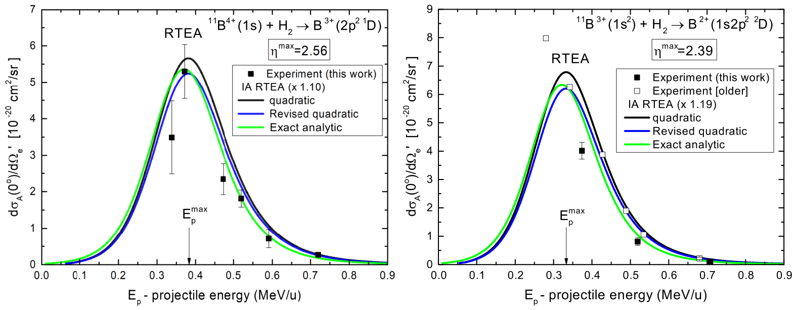
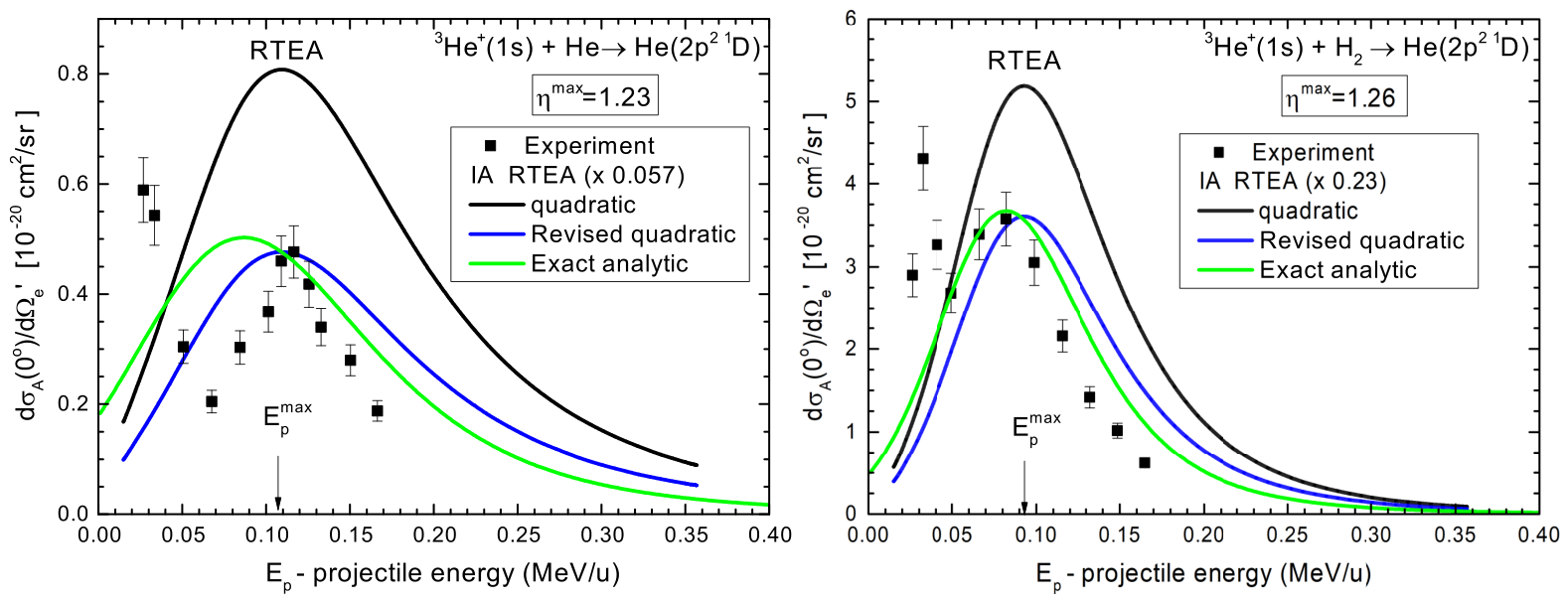
In Figure 5, Figure 6 and Figure 7, we compare the three IA SDCS models with experimental zero-degree data (data points). These include the revised quadratic IA (blue lines) and older quadratic IA (black lines) from Equation (59), and the exact IA (green lines) from Equation (64). To assess theory–experiment agreement, we define the scaling factor r as the ratio of the experimental to theoretical maximum SDCS (using the revised quadratic IA from Equation (68)):
r d σ Exp max d Ω e ( 0 ) d σ R T E A max d Ω e ( 0 ) .
This ratio allows for the extraction of an empirical collision strength, Ω R E Exp , given by:
Ω R E Exp r Ω R E ,
where Ω R E is the theoretical RE collision strength from Equations (6) and (11). Available RTEA SDCS measurements and their resulting Ω R E Exp and r values are summarized in Table 2, Table 3 and Table 4.
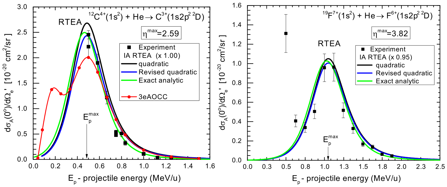
All three IA calculations in the figures are scaled by r, determined by normalizing the revised quadratic IA (blue lines) to the experimental peak according to Equation (77). The exact analytic IA (green) is seen to exhibit a marginally better overall agreement with the data. It is also slightly shifted toward lower energies relative to the quadratic prediction E p max (Equation (71)), reflecting the 1 / V p dependence in the exact SDCS (Equation (64)).
In the quadratic model, this V p denominator is replaced by the constant 2 ϵ R / m (Equation (59)). Despite this qualitative difference, the resulting SDCS remain remarkably similar because the V p dependence is largely compensated by the differing p R definitions (Equations (43) and (47)) within the Compton profile. This additional 1 / V p factor in the non-quadratic models tends to slightly increase the cross-sections and shift the SDCS maximum toward lower velocities. In this case, the maximum can only be calculated numerically. Although the linear treatment is considered inferior to the quadratic model [11,30,44], its derivation is included here for completeness (Equation (61)). Originally derived by Brandt [9], this linear IA justifiably neglected the target ionization energy E I (i.e., set E I = 0 ) to focus on the RTEX measurements of that period, which involved high- Z p ions ( Z p > 10 ) where E a E I .
Figure 5 and Figure 6 demonstrate the agreement between the three zero-degree IA RTEA SDCS calculations and experimental data for 1s2p2 2D and 2p2 1D state production in He-like and H-like C, F, and B ions. At the lowest collision energies, the observed increase in the experimental SDCS is due to NTE, which is not handled by the IA.
He-like ion beams contain a mixture of ground ( 1 s 2 ) and metastable ( 1 s 2 s ) states, complicating absolute SDCS determination. We utilize an in situ gas-stripping technique at the tandem accelerator terminal to preferentially produce ground-state ions [138] and determine the ground-state fraction f g [139]. Since 1s2p2 2D production occurs almost exclusively from ground-state ions in this range, experimental SDCS were corrected by 1 / f g .
The revised quadratic IA (blue lines) is seen to be systematically smaller than the original quadratic treatment (black lines) due to the E a / ( E a + E I ) target ionization correction factor. This correction, also featured in the exact analytic IA, yields improved absolute agreement with experiment, most pronounced for lower- Z p ions where E a is smaller. This effect is particularly evident in Figure 7 for He++He/H2, though the IA validity here is questionable ( V p v , η max = 1.23 ), as evidenced by the much smaller r values and profile discrepancies. While the IA still predicts the RTE peak energy E p max fairly reasonably, the criterion η max 1 is clearly violated.
In Figure 8, a DDCS comparison with the R-matrix is also presented, showing impressive agreement between the two. By integrating the areas under the 2p2 1D peak, Auger SDCS were obtained for both experiment and theory, from which the RE collision strengths, Ω R E , were computed. These extracted Ω R E values are listed in Table 2 (but in parentheses) and are compared to our present IA calculations.
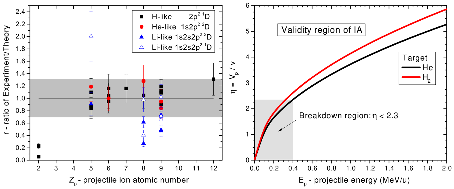
Finally, in Figure 9, the scaling factor r is plotted as a function of Z p for each collision system. Agreement with experiment is seen to be very good, lying within the constant r = 1 grey zone with an absolute uncertainty up to 30 % across most Z p —unlike the systematic disagreement with decreasing Z p reported previously (see Figure 8 in [43]). That earlier discrepancy showed a very similar Z p -dependency to the correction factor trend now illustrated in Figure 2. It is clear that the observed improvement in the r  Z p -dependency stems primarily from this newly applied correction factor. Nevertheless, more accurate Auger rates A a available since the early 1990s and used in the calculation of Ω R E (see Table 2, Table 3 and Table 4) are also partly responsible for this improved agreement. For instance, the carbon calculations in Figure 5 utilize a modern Z-expansion rate ( A a = 0.756 × 10 14 s−1) [113] rather than the older MCDF value ( 0.932 × 10 14 s−1) [140] used in previous work [19]. For Z p = 2 (He+), the large discrepancy r = 0.23 for collisions with H2 reflects the IA breakdown ( V p v and not V p v ), yet astonishingly the scaled IA RTEA SDCS profiles still closely match the data [Figure 7 (right)].
Remarkably, just a simple overall one-parameter scaling by r seems to suffice for most systems (including boron H-like and He-like ions), suggesting robust target Compton profile integrity during collisions ( Φ ( p ) Φ i ( p ) , Equation (27) as already pointed out, a key feature of the IA. Any disagreement trends therefore likely reflect increasing projectile disturbance by the target as their electron binding weakens. H-like and He-like ions have the tightest bound K-shell electrons and show the best agreement; Li-like systems—with the more loosely bound 2 s spectator electron—deviate more [10]. This is particularly evident for the 1s2s2p2 1D state where ξ is also uniquely much less than 1 (see Table 4), potentially signaling less accurate multi-electron A a and ξ values. However, this conjecture seems to be in conflict with the concept of “ion surgery” for fast light targets in collision with multi-electron ions [141]. Accordingly, low Z t targets (e.g., He/H2) act as a “needle”, selectively ionizing the projectile inner shell without substantially disturbing the outer shells, which are thus preserved as evidenced by the limited number of charge states produced in the collision [126], in contrast to collisions with heavier targets. Clearly, RTEA investigations of Be- and B-like ions with even more spectator electrons might be able to shed more light on this. In addition, the 1s2s2p2 3,1D states are more complicated since they can Auger decay either to the 1s22s or the 1s22p final states. Clearly, these complication are absent for the 2p2 1D and 1s2p2 2D states and might also be responsible for their borderline behavior.
Further investigation into how and why the IA breaks down would thus be of interest. In particular, RTEA measurements of Li+ and Li2+ He ions, not undertaken to date, should lie near the limit of the IA validity ( η max 1.4 ) and would therefore also be interesting. In Table 2 and Table 3, we have listed expected values of lithium Ω R E and d σ R T E A max ( 0 ) / d Ω e for future reference. Overall, the systematic analysis reported here for the D states indicates that the IA seems to be valid even when V p is only a bit larger than v , i.e., for η 2.3 as shown in Figure 9 (right).
Finally, in Figure 5 for carbon (left) the first rigorous ion–atom collision calculations of RTE are shown. This treatment focused on the production of the C3+(1s2p2 2D) state via the process
C 4 + ( 1 s 2 ) + He C 3 + ( 1 s 2 p 2   D 2 ) + He + ( transfer excitation )
C 4 + ( 1 s 2 ) + e A ( θ e = 0 ) , ( 0 Auger stabilization )
with the Auger SDCS determined via ZAPS [107] by detecting the 2D Auger electron at θ e = 0 relative to the ion beam direction. This full configuration interaction, semiclassical close-coupling approach [59] considers the dynamics of three active electrons (known as 3eAOCC)—two on the projectile and one on the target—with the second He target electron considered to be frozen. This approach allows for a coupled and coherent treatment of all processes, such as target and projectile excitation, ionization, single electron capture, as well as all TE processes (RTE, NTE, etc.) and therefore go well beyond the methods developed in the past. Two peaks are observed in the computed SDCS (Figure 5 red line). The high-energy peak is seen to be in very good agreement with experiment at/above resonance (0.5 MeV/u), confirming RTE dominance via two-center ( e - e ) interactions at large impact parameters b [19]. Notably, our analysis reveals that the low-energy peak—situated below 0.375 MeV/u where measurements remain unattainable (outside the tandem accelerator range)—arises from a direct one-step interaction during head-on collisions (small b). This challenges the conventional interpretation of a two-step non-resonant transfer excitation (NTE) process. We designate this mechanism as non-correlated transfer excitation (NCTE) [19]. This quantum mechanical treatment provides fresh insight into bielectronic processes within many-body systems; however, experimental validation for this low-energy mechanism is currently pending. We are in the process of further testing the accuracy of the 3eAOCC calculations for other low- Z p isoelectronic systems. A 4eAOCC treatment is also underway to test the validity of the independent electron approximation used for the He target.
As a final note, we mention that S and P states, while observable, exhibit much smaller RTE cross-sections that are difficult to measure accurately; consequently, investigations have focused almost exclusively on D states. This is consistent with the ( 2 L j + 1 ) 2 scaling of the zero-degree SDCS (seen in Equation (66)), which significantly favors states with higher orbital angular momentum.

6. Summary and Conclusions

We have reviewed the progress of resonant transfer excitation followed by Auger stabilization (RTEA) investigations since the comprehensive review of 1992 [43]. We continue to focus on state-resolved single differential cross-section (SDCS) measurements of the most strongly populated KLL D states obtained through zero-degree Auger projectile spectroscopy (ZAPS).
These state-selective SDCS measurements enable simple, direct comparisons with the impulse approximation (IA) predictions while providing its most stringent tests. The IA predictions rely primarily upon well-established atomic structure parameters available in the literature. Prior to 1992, 14 such measurements were reported—some employing disparate absolute calibration methods and non-uniform treatment of the Auger angular dependence. The 1992 review revealed a systematic discrepancy where IA predictions were consistently larger than the experimental SDCS ( r < 1 ), with r dropping with decreasing Z p , casting some doubts on the impulse approximation’s validity, particularly for low- Z p ions.
Since that time, an additional 16 RTEA measurements have been reported, including several new collision systems presented here. These later experiments benefit from standardized absolute detection efficiency calibration using the IA binary encounter electron peak (nonresonant elastic scattering). For He-like ion beams, which contain mixtures of ground and metastable states, a more accurate in situ determination of the ground-state fraction has also been implemented. Moreover, the original two-stage parallel-plate spectrometer has been superseded by the single-stage hemispherical deflector spectrograph that offers two orders of magnitude greater efficiency. Taken together, these experimental advances have yielded significantly more reliable and accurate experimental SDCS.
We have revisited the fundamental connection between the electron–ion process of dielectronic capture (DC) and its ion–atom counterpart, RTE, provided by the IA. Our systematic comparison of RTEA SDCS—now computed using more accurate Auger rates while uniformly accounting for the highly anisotropic Auger emission at zero-degree observation and target ionization energy corrections—demonstrates excellent agreement with practically all available measurements spanning both pre- and post-1992 eras. In addition, we have also presented a new exact analytic IA treatment which is shown to be in even better agreement than the revised quadratic IA results. Most importantly, no systematic discrepancy remains. The IA’s validity is now firmly established down to boron for H-like and He-like ions, with He+ representing the sole clear exception where IA breakdown occurs as expected. Remarkably, the IA is found to be valid down to η 2.3 , clearly much lower than what would be expected by the generally assumed IA validity criterion of η 1 . However, some Li-like ion cases seem to be on the borderline for reasons not clearly understood. Overall, these results confirm that state-selective RTEA measurements in combination with the IA can serve as a uniquely reliable source of Auger rates and yields, essential for computing DC/RE/DR collision strengths used in plasma modeling.
Over the last four decades, ZAPS has delivered the most accurate state-selective SDCS measurements for low- Z p ion–atom collision processes, leading the way in the investigations of RTE. Very recently, nonperturbative 3eAOCC transfer excitation calculations have also emerged. Excellent agreement was observed with carbon 1s2p2 2D ZAPS data near the RTE peak. Furthermore, a mechanism, distinct from conventional NTE, was revealed at lower energies, which, however, remains to be experimentally verified. Ongoing experimental/theoretical isoelectronic studies promise new insights into many-body quantum dynamics under intense, ultra-fast perturbations. In addition, RTEA studies of Li+ and Li2+ collisions with He/H2 would provide valuable tests of IA validity. Moreover, investigating KLL RTEA for Be-like and B-like ions would further examine IA applicability to projectiles with multiple spectator electrons, possibly shedding more light on the role of spectator electrons during the collision, as already seen for Li-like ions. Finally, Coster–Kronig (CK) transitions in much heavier ions could also be explored using electrostatic analyzers. For example, the L 1 L 3 M 5 CK transition yields electron energies of about 340 eV for lead ions and 1039 eV for uranium ions with extremely high Auger rates, which have never been explored and could well be of RTE interest.


Author Contributions

Conceptualization, T.J.M.Z.; methodology, T.J.M.Z. and E.P.B.; software, T.J.M.Z.; formal analysis, T.J.M.Z. and E.P.B.; investigation, T.J.M.Z. and E.P.B.; data curation, T.J.M.Z.; writing—original draft preparation, T.J.M.Z.; writing—review and editing, T.J.M.Z. and E.P.B.; visualization, T.J.M.Z. and E.P.B. All authors have read and agreed to the published version of the manuscript.

Funding

This research received no external funding.

Data Availability Statement

The data presented in this study are available upon request from the corresponding author.

Acknowledgments

We thank Sotiris Harissopulos, former director of the NCSR “Demokritos” Tandem accelerator, for his more than decade-long support during the ZAPS setup, installation and commissioning. We also thank the accelerator staff for their maintenance, upgrades, and assistance with the measurements. Finally, we express our deep gratitude to Alain Dubois (and his group) at Sorbonne University, Paris, for his warm friendship, enthusiasm in advancing the 3eAOCC codes, and invaluable physics discussions throughout our collaboration.

Conflicts of Interest

The authors declare no conflicts of interest.

Abbreviations

2Dtwo-dimensional
3eAOCCthree-electron atomic orbital close-coupling
3eASCCthree-electron asymptotic state close-coupling
AOCCatomic orbital close-coupling
ASCCasymptotic state close-coupling
BEebinary encounter electrons
CKCoster–Kronig
DCdielectronic capture
DDCSdouble-differential cross-section d 2 σ / d Ω e d ε
DRdielectronic recombination
EBISelectron beam ion source
EBITelectron beam ion trap
ESMelectron scattering model
FCFaraday cup
GSIGesellschaft für Schwerionenforschung
HDAhemispherical deflector analyzer
IAimpulse approximation
ITERinternational thermonuclear experimental reactor
LTElocal thermodynamic equilibrium
NCTEnon-correlated transfer and excitation
NCSRnational center for scientific research
NESRnew experimental storage ring at GSI
NTEnonresonant transfer and excitation
PSDposition sensitive detector
RCradiationless capture
REresonant excitation
RRradiative recombination
RTEresonant transfer and excitation
RTEAresonant transfer and excitation followed by Auger electron emission
RTEXresonant transfer and excitation followed by X-ray emission
SDCSsingle differential cross-section d σ / d Ω e
SRstorage ring
TEtransfer excitation
ZAPSzero-degree Auger projectile spectroscopy

Appendix A. Compton Profile Parameterizations of H2 and He

The Compton profile, J ( p z ) , represents the momentum distribution, along the z-axis [97,142]:
J ( p z ) = d p x d p y | Ψ ( p ) | 2 ,
where Ψ ( p ) is the target momentum wave function.
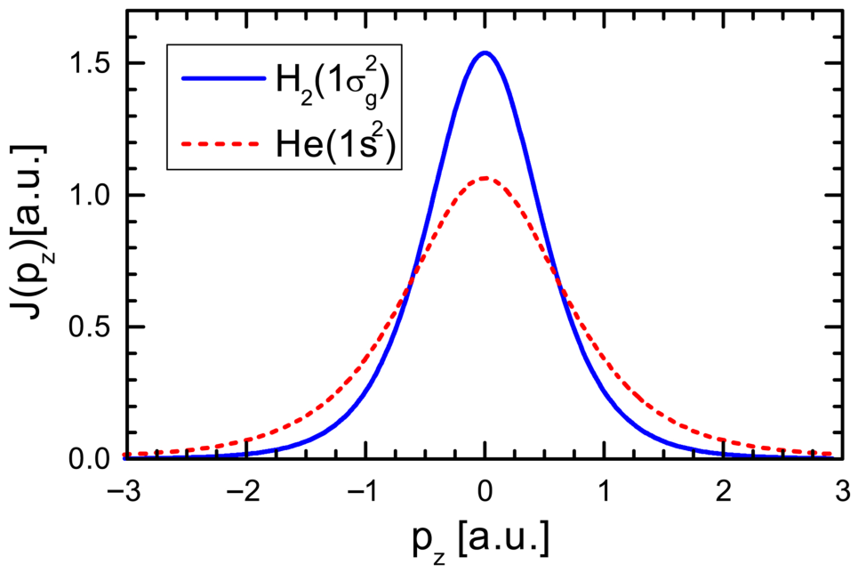
The Compton profile is usually determined independently, either theoretically or experimentally [100,142]. In Figure A1, a few characteristic distributions are shown. In general, the width of the distribution is related to the electron binding energy.
Figure A1. Compton profiles J ( p z ) for H2 and He targets.
Atoms 14 00038 g0a1
For H2 and He targets, the experimentally measured Compton profile is given by the following analytic expression [100]:
J ( p z ) = n = 1 N a n [ 1 + ( p z / ξ n ) 2 ] n + 2 ,
where the a n and ξ n coefficients are given in Table A1 and J ( p z ) has been normalized so that,
J ( p z ) d p z = 2 ,
the number of electrons in the ground state.
The Compton profiles of H2 and He using Equation (A2) are plotted in Figure A1. From Table A1 for p z = 0 , we readily find J ( 0 ) = 1.5395 a.u. (H2) and 1.0641 a.u. (He).
Table A1. a n and ξ n coefficients for the H2 and He Compton profiles (see Equation (A2)).
J(pz) Coefficients
H2 Target He Target
n a n ξ n n a n ξ n
11.00120.98961−0.09572.1828
20.53831.556620.05144.1598
30.13423.5200
40.73162.3948
50.24261.5732

Appendix B. Analytic Evaluation of the Double Integral I10 (Vp, ϵR) in the Exact IA

The analytical solution for the double integral I 10 ( V p , ϵ R ) defined in Equation (54) as:
I 10 ( V p , ϵ R ) ϵ R 0 | F 10 ( p ) | 2 1 1 d z L Γ j ( ϵ ( V p , z , p ) ϵ R ) ϵ ( V p , z , p ) p 2 d p ,
with the ground-state form factor | F 10 | 2 given by Equation (52) as:
| F 10 ( p ) | 2 = 2 5 π ( Z t p 0 ) 5 [ p 2 + ( Z t p 0 ) 2 ] 4 ,
we have:
I 10 ( V p , ϵ R ) = 16 3 π V p Z t p 0 1 p ˜ 2 + 1 3 1 p ˜ + 2 + 1 3 ,
where the momentum limits p ˜ ± are:
p ˜ ± = m V p ± 2 m ϵ R Z t p 0 .
In atomic units (a.u.), this expression simplifies to:
I 10 ( V p , ϵ R ) [ a . u . ] = 16 3 π V p [ a . u . ] Z t 1 ( p ˜ [ a . u . ] 2 + 1 ) 3 1 ( p ˜ + [ a . u . ] 2 + 1 ) 3 ,
with
p ˜ ± [ a . u . ] = V p [ a . u . ] ± 2 ϵ R [ a . u . ] Z t .
Here, the projectile velocity V p in a.u. is determined from the projectile energy E p via Equation (67).
To derive this result, we follow a three-step procedure:

Appendix B.1. Step 1: Simplify the Inner Integral Using the Delta Function Approximation

We approximate the Lorentzian distribution as a delta function, L Γ j ( Δ ϵ ) δ ( Δ ϵ ) , which is valid since the width Γ j is much smaller than the energy difference. The inner integral with respect to z (from Equation (54)) becomes:
I z = 1 1 d z δ ( ϵ ( V p , z , p ) ϵ R ) ϵ ( V p , z , p ) .
The delta function δ ( g ( z ) ) contributes only at the root z 0 where ϵ ( V p , z 0 , p ) = ϵ R . Given the relation ϵ ( V p , z , p ) = 1 2 m V p 2 + p 2 2 m + V p z p (Equation (49)), we find:
z 0 = ϵ R 1 2 m V p 2 p 2 2 m V p p .
Using the property δ ( g ( z ) ) = δ ( z z 0 ) / | g ( z 0 ) | , where | g ( z 0 ) | = | ϵ / z | = V p p , the inner integral evaluates to:
I z = 1 V p p ϵ R for z 0 [ 1 , 1 ] .

Appendix B.2. Step 2: Determine the Limits of the Outer Integral

The requirement that the root must fall within the physical domain ( 1 z 0 1 ) restricts the contributing momentum p. This condition is expressed as:
ϵ R 1 2 m V p 2 p 2 2 m V p p .
Solving for p yields the integration range [ p , p + ] , where:
p ± = m V p ± 2 m ϵ R .

Appendix B.3. Step 3: Evaluate the Outer Integral over p

Substituting I z and the hydrogenic form factor | F 10 ( p ) | 2 (Equation (A5)) into the expression for I 10 (Equation (A4)), we obtain:
I 10 = 2 5 ( Z t p 0 ) 5 V p π p p + p [ p 2 + ( Z t p 0 ) 2 ] 4 d p .
Using the substitution u = p 2 + ( Z t p 0 ) 2 , the antiderivative is 1 / ( 6 u 3 ) . Evaluating across the limits [ p , p + ] gives:
I 10 ( V p , ϵ R ) = 16 3 π V p Z t p 0 1 p Z t p 0 2 + 1 3 1 p + Z t p 0 2 + 1 3 .
With V p and p ˜ ± in atomic units, we have:
I 10 = 16 3 π ε 0 V p [ a . u . ] Z t 1 ( p ˜ 2 + 1 ) 3 1 ( p ˜ + 2 + 1 ) 3 ,
with
p ˜ ± = p ± [ a . u . ] Z t = V p [ a . u . ] ± 2 ϵ R [ a . u . ] Z t .

Appendix B.4. Maximum Value of the Integral I10

The integral reaches its maximum when p = 0 , which corresponds to a projectile velocity V p max = 2 ϵ R / m . This is consistent with the approximate Impulse Approximation (IA) formulas. At this maximum, p ˜ + ( V p max ) = 2 2 ϵ R [ a . u . ] / Z t . Substituting this into Equation (A17) gives:
I 10 max [ a . u . ] = 16 3 π Z t 2 ϵ R [ a . u . ] 1 1 ( 8 ϵ R [ a . u . ] Z t 2 + 1 ) 3 .
Neglecting the second term in the brackets (as it is typically much smaller than unity), we find:
I 10 max [ a . u . ] 16 3 π Z t 2 ϵ R [ a . u . ] .
Substituting Equation (A20) into the exact IA RTEA SDCS (Equation (63)), the maximum cross-section is:
d σ R T E A exact d Ω e max = d σ R E ( 0 ) d Ω e E a E a + E I 16 3 π Z t 2 ϵ R [ a . u . ] .
To compare this with the revised quadratic RTEA SDCS, we take the ratio
d σ R T E A exact / d Ω e max d σ R T E A max / d Ω e = 16 3 π Z t J ( 0 ) [ a . u . ] 1.6977 Z t J ( 0 ) [ a . u . ] .
Using the values for J ( 0 ) and Z t from Table 1 for H2 and He, we find this ratio to equal 1. Thus, Z t can be determined directly as:
Z t = 16 3 π J ( 0 ) [ a . u . ] .

References

  1. Vrakking, M.J.J.; Lepine, F. (Eds.) Attosecond Molecular Dynamics; Theoretical and Computational Chemistry Series; The Royal Society of Chemistry: London, UK, 2018; pp. 1–37. [Google Scholar] [CrossRef]
  2. Tao, Z.; Chen, C.; Szilvási, T.; Keller, M.; Mavrikakis, M.; Kapteyn, H.; Murnane, M. Direct time-domain observation of attosecond final-state lifetimes in photoemission from solids. Science 2016, 353, 62–67. [Google Scholar] [CrossRef]
  3. Clark, M.; Brandt, D.; Swenson, J.K.; Shafroth, S.M. Nonresonant Electron Transfer and Projectile K-Electron Excitation in Ion-Atom Collisions. Phys. Rev. Lett. 1985, 54, 544–546. [Google Scholar] [CrossRef] [PubMed]
  4. Tanis, J.A.; Bernstein, E.M.; Clark, M.W.; Graham, W.G.; McFarland, R.H.; Morgan, T.J.; Johnson, B.M.; Jones, K.W.; Meron, M. Evidence for uncorrelated electron capture and K-shell excitation in S13+ + He collisions. Phys. Rev. A 1985, 31, 4040–4042. [Google Scholar] [CrossRef] [PubMed]
  5. Tanis, J.A.; Bernstein, E.M.; Graham, W.G.; Clark, M.; Shafroth, S.M.; Johnson, B.M.; Jones, K.W.; Meron, M. Resonant Behavior in the Projectile X-ray Yield Associated with Electron Capture in S+Ar Collisions. Phys. Rev. Lett. 1982, 49, 1325–1328. [Google Scholar] [CrossRef]
  6. Tanis, J.A.; Bernstein, E.M.; Graham, W.G.; Stöckli, M.P.; Clark, M.; McFarland, R.H.; Morgan, T.J.; Berkner, K.H.; Schlachter, A.S.; Stearns, J.W. Resonant Electron Transfer and Excitation in Two-, Three-, and Four- Electron 20Caq+ and 23Vq+ Ions Colliding with Helium. Phys. Rev. Lett. 1984, 53, 2551–2554. [Google Scholar] [CrossRef]
  7. Pepmiller, P.L.; Prichard, R.; Newcomb, J.; Dillingham, R.; Hall, J.M.; Gray, T.J.; Stöckli, M. A study of transfer excitation in F8++He, Ne and Ar collisions. IEEE Trans. Nucl. Sci. 1983, NS-30, 1002. [Google Scholar] [CrossRef]
  8. Brandt, D. A simple classical model for the impact parameter dependence of electron capture. Nucl. Instrum. Methods 1983, 214, 93–96. [Google Scholar] [CrossRef]
  9. Brandt, D. Resonant Transfer and Excitation in ion-atom collisions. Phys. Rev. A 1983, 27, 1314–1318. [Google Scholar] [CrossRef]
  10. Swenson, J.K.; Yamazaki, Y.; Miller, P.D.; Krause, H.F.; Dittner, P.F.; Pepmiller, P.L.; Datz, S.; Stolterfoht, N. Observation of Resonant Transfer and Excitation to Specific LS-Coupled States in O5+ + He Collisions by High-Resolution, 0° Auger-Electron Spectroscopy. Phys. Rev. Lett. 1986, 57, 3042–3045. [Google Scholar] [CrossRef]
  11. Zouros, T.J.M.; Lee, D.H.; Richard, P.; Sanders, J.M.; Shinpaugh, J.L.; Varghese, S.L.; Karim, K.R.; Bhalla, C.P. State-Selective Observation of Resonance Transfer Excitation (RTE) in Collisions of F6+ with He and H2 Targets. Phys. Rev. A 1989, 40, 6246–6250. [Google Scholar] [CrossRef]
  12. Benis, E.P.; Zouros, T.J.M.; Gorczyca, T.W.; González, A.D.; Richard, P. Elastic resonant and nonresonant differential scattering of quasifree electrons from B4+(1s) and B3+(1s2) ions. Phys. Rev. A 2004, 69, 052718, Erratum in Phys. Rev. A 2006, 73, 029901. [Google Scholar] [CrossRef]
  13. Fritsch, W.; Lin, C.D. Analysis of Electron Correlation in Simultaneous Eletron Transfer and Excitation in Atomic Collisions. Phys. Rev. Lett. 1988, 61, 690–693. [Google Scholar] [CrossRef] [PubMed]
  14. Feagin, J.M.; Briggs, J.S.; Reeves, T.M. Simultaneous charge transfer and excitation. J. Phys. B 1984, 17, 1057–1068. [Google Scholar] [CrossRef]
  15. Itoh, A.; Zouros, T.J.M.; Schneider, D.; Stettner, U.; Zeitz, W.; Stolterfoht, N. Transfer Excitation in He++He Collisions Studied by Zero-Degree Electron Spectroscopy. J. Phys. B 1985, 18, 4581–4587. [Google Scholar] [CrossRef]
  16. Benhenni, M.; Shafroth, S.M.; Swenson, J.K.; Schulz, M.; Giese, J.P.; Schöne, H.; Vane, C.R.; Dittner, P.F.; Datz, S. Angular distribution of Auger electrons emitted through the resonant transfer and excitation process following O5++He collisions. Phys. Rev. Lett. 1990, 65, 1849–1852. [Google Scholar] [CrossRef]
  17. Benhenni, M.; Shafroth, S.M.; Swenson, J.K. Alignment in fast ion-atom collisions. Nucl. Instrum. Methods B 1994, 86, 28–37. [Google Scholar] [CrossRef]
  18. Ourdane, M.; Bachau, H.; Gayet, R.; Hanssen, J. Transfer and excitation in high-energy He+-He collisions: V. Electronic continuum influence on ejected electron distributions and TE cross-sections. J. Phys. B 1999, 32, 2041–2055. [Google Scholar] [CrossRef]
  19. Laoutaris, A.; Nanos, S.; Madesis, I.; Passalidis, S.; Benis, E.P.; Dubois, A.; Zouros, T.J.M. Coherent treatment of transfer-excitation processes in swift ion-atom collisions. Phys. Rev. A 2022, 106, 022810. [Google Scholar] [CrossRef]
  20. Tanis, J.A.; Shafroth, S.M.; Willis, J.E.; Clark, M.; Swenson, J.; Strait, E.N.; Mowat, J.R. Simultaneous Electron Capture and Excitation in S+Ar Collisions. Phys. Rev. Lett. 1981, 47, 828–831. [Google Scholar] [CrossRef]
  21. Graham, W.G.; Fritsch, W.; Hahn, Y.; Tanis, J. (Eds.) Recombination of Atomic Ions; NATO Advanced Study Institute Series B: Physics; Springer: Boston, MA, USA, 1992; Volume 296. [Google Scholar] [CrossRef]
  22. Müller, A. Electron-Ion Collisions: Fundamental Processes in the Focus of Applied Research. Adv. At. Mol. Opt. Phys. 2008, 55, 293–417. [Google Scholar] [CrossRef]
  23. Williams, I.D. Electron-ion scattering. Rep. Prog. Phys. 1999, 62, 1431–1469. [Google Scholar] [CrossRef]
  24. Crawford, E.; Sime, R.L.; Walker, M. A Nobel Tale of Postwar Injustice. Phys. Today 1997, 50, 26–32. [Google Scholar] [CrossRef]
  25. Matsakis, D.; Coster, A.; Laster, B.; Sime, R. A renaming proposal: “The Auger–Meitner effect”. Phys. Today 2019, 72, 10–11. [Google Scholar] [CrossRef]
  26. Duparc, O.H. Pierre Auger—Lise Meitner: Comparative contributions to the Auger effect. Int. J. Mat. Res. 2009, 100, 1162–1166. [Google Scholar] [CrossRef]
  27. Hahn, Y.; Lagattuta, K.J. Dielectronic recombination and related resonance processes. Phys. Rep. 1988, 166, 195–268. [Google Scholar] [CrossRef]
  28. Pradhan, A.K.; Nahar, S.N. Atomic Astrophysics and Spectroscopy; Cambridge University Press: Cambridge, UK, 2011. [Google Scholar]
  29. Bhalla, C.P. Angular distribution of Auger electrons and photons in resonant transfer and excitation in collisions of ions with light targets. Phys. Rev. Lett. 1990, 64, 1103–1106. [Google Scholar] [CrossRef]
  30. Lee, D.H.; Richard, P.; Zouros, T.J.M.; Sanders, J.M.; Shinpaugh, J.L.; Hidmi, H. Binary Encounter Electrons Observed at Zero Degrees in Collisions of 1–2 MeV/amu H+, C6+, N7+, O8+ and F9+. Phys. Rev. A 1990, 41, 4816–4823. [Google Scholar] [CrossRef]
  31. Závodszky, P.A.; Tóth, G.; Grabbe, S.R.; Zouros, T.J.M.; Richard, P.; Bhalla, C.P.; Tanis, J.A. Forward-backward asymmetry in the inelastic scattering of electrons from highly charged ions. J. Phys. B 1999, 32, 4425–4435. [Google Scholar] [CrossRef]
  32. Zouros, T.J.M.; Lee, D.H.; Richard, P. Projectile 1s→2p Excitation Due to Electron-Electron Interaction in Collisions of O5+ and F6+ Ions with H2 and He Targets. Phys. Rev. Lett. 1989, 62, 2261–2264. [Google Scholar] [CrossRef]
  33. Montenegro, E.C.; Melo, W.S.; Meyerhof, W.E.; de Pinho, A.G. Separation of the Screening and Antiscreening Effects in the Electron Loss of He+ on H2 and He. Phys. Rev. Lett. 1992, 69, 3033–3036. [Google Scholar] [CrossRef]
  34. Lee, D.H.; Zouros, T.J.M.; Sanders, J.M.; Richard, P.; Anthony, J.M.; Wang, Y.D.; McGuire, J.H. K-shell Ionization of O4+ and C2+ ions in fast collisions with H2 and He gas targets. Phys. Rev. A 1992, 46, 1374–1387. [Google Scholar] [CrossRef]
  35. Závodszky, P.A.; Aliabadi, H.; Bhalla, C.P.; Richard, P.; Tóth, G.; Tanis, J.A. Superelastic scattering of electrons from highly charged ions with inner shell vacancies. Phys. Rev. Lett. 2001, 87, 033202. [Google Scholar] [CrossRef] [PubMed]
  36. Montenegro, E.C.; Meyerhof, W.E. Passive and Active Electrons in the Electron Loss Process. In Two-Center Effects in Ion-Atom Collisions; AIP Conference Proceedings; Gay, T.J., Starace, A.F., Eds.; American Institute of Physics: New York, NY, USA, 1995; Volume 362, pp. 103–112. [Google Scholar]
  37. Zouros, T.J.M. Projectile-electron - target-electron interactions: Exposing the dynamic role of electrons in fast ion-atom collisions. Comments At. Mol. Phys. 1996, 32, 291–313. [Google Scholar]
  38. Montenegro, E.C.; Zouros, T.J.M. On the relationship between the Born and the impulse approximations for the antiscreening process. Phys. Rev. A 1994, 50, 3186–3191. [Google Scholar] [CrossRef] [PubMed]
  39. Tanis, J.; Graham, W.; Berkner, K.; Bernstein, E.; Clark, M.; Feinberg, B.; McMahan, M.; Morgan, T.; Rathbun, W.; Schlachter, A. Resonant transfer excitation in U89+ + C and U90+ + H2 collisions. Nucl. Instrum. Methods B 1991, 53, 442–447. [Google Scholar] [CrossRef]
  40. Mokler, P.H.; Reusch, S.; Warczak, A.; Stachura, Z.; Kambara, T.; Müller, A.; Schuch, R.; Schulz, M. Single transfer-excitation resonance observed via the two-photon decay in He-like Ge30+. Phys. Rev. Lett. 1990, 65, 3108–3111. [Google Scholar] [CrossRef]
  41. Tanis, J.A. Resonant Transfer Excitation Associated with Single X-ray Emission. In Recombination of Atomic Ions; Graham, W.G., Fritsch, W., Hahn, Y., Tanis, J., Eds.; NATO Advanced Study Institute Series B: Physics; Springer: Boston, MA, USA, 1992; Volume 296, pp. 241–257. [Google Scholar] [CrossRef]
  42. Ding, T.; Xie, L.; He, W.; Rui, J.; Ma, Y.; Liu, Y.; Dong, C. Theoretical study on resonant transfer and excitation process of hydrogen-like and helium-like ions. Eur. Phys. J. D 2025, 79, 101. [Google Scholar] [CrossRef]
  43. Zouros, T.J.M. Resonant Transfer and Excitation Associated with Auger Electron Emission. In Recombination of Atomic Ions; Graham, W.G., Fritsch, W., Hahn, Y., Tanis, J., Eds.; NATO Advanced Study Institute Series B: Physics; Springer: Boston, MA, USA, 1992; Volume 296, pp. 271–300. [Google Scholar] [CrossRef]
  44. Zouros, T.J.M.; Bhalla, C.P.; Lee, D.H.; Richard, P. Effects of Alignment and Interference in Resonant Transfer and Excitation for F6+ and O5+ Collisions with H2 in 0° Auger Measurements. Phys. Rev. A 1990, 42, 678–681. [Google Scholar] [CrossRef]
  45. DePaola, B.D.; Parameswaran, R.; Axmann, W.J. High-resolution state-selective study of transfer with excitation in the F8++H2 system. Phys. Rev. A 1990, 41, 6533–6535. [Google Scholar] [CrossRef]
  46. DePaola, B. RTE studied in electron emission. Nucl. Instrum. Methods B 1991, 56-57, 154–157. [Google Scholar] [CrossRef]
  47. Lee, D.H.; Richard, P.; Sanders, J.M.; Zouros, T.J.M.; Shinpaugh, J.L.; Varghese, S.L. KLL resonant transfer and excitation to F6+(1s2l2l) intermediate states. Phys. Rev. A 1991, 44, 1636–1643. [Google Scholar] [CrossRef]
  48. Parameswaran, R.; Bhalla, C.P.; Walch, B.P.; DePaola, B.D. Resonant transfer and excitation in collisions of C5+ with H2 and He targets. Phys. Rev. A 1991, 43, 5929–5933. [Google Scholar] [CrossRef] [PubMed]
  49. Burke, P.G.; Berrington, K.A. Atomic and Molecular Processes: An R-Matrix Approach; Institute of Physics Publishing: Bristol, UK; Philadelphia, PA, USA, 1993. [Google Scholar]
  50. Bray, I.; Hayat, H.; Fursa, D.V.; Kadyrov, A.S.; Bray, A.W.; Cytowski, M. Calculations of electron scattering on H-like ions. Phys. Rev. A 2020, 101, 022703. [Google Scholar] [CrossRef]
  51. Stolterfoht, N. Dielectronic processes and electron correlation in energetic ion-atom collisions. Nucl. Instrum. Methods B 1991, 53, 477–492. [Google Scholar] [CrossRef]
  52. Bachau, H.; Gayet, R.; Hanssen, J.; Zerarka, A. Transfer and excitation in ion-atom collisions at high impact velocities: A unified continuum distorted wave treatment of resonant and non-resonant modes in four body approach: II. Application to the collisions S15+(1s) + H(1s). J. Phys. B 1992, 25, 839–852. [Google Scholar] [CrossRef]
  53. Gayet, R.; Hanssen, J. Resonant and non-resonant modes of transfer and excitation processes in ion-atom collisions. Nucl. Instrum. Methods B 1994, 86, 52–61. [Google Scholar] [CrossRef]
  54. Gayet, R.; Hanssen, J.; Jacqui, L. Transfer and excitation in ion-atom collisions at high impact velocities: III. Application of the CDW-4B theory to an almost symmetrical system: He++He. J. Phys. B 1995, 28, 2193–2208. [Google Scholar] [CrossRef]
  55. Gayet, R.; Hanssen, J.; Jacqui, L.; Ourdane, M.A. Transfer and excitation in ion-atom collisions at high impact velocities: IV. Application of the CDW-4B theory to an almost symmetrical system: He++H. J. Phys. B 1997, 30, 2209–2219. [Google Scholar] [CrossRef]
  56. Zouros, T.J.M.; Schneider, D.; Stolterfoht, N. State-selective observation of resonant and non-resonant transfer excitation in 50–500 keV 3He++H2 collisions. J. Phys. B 1988, 21, L671–L676. [Google Scholar] [CrossRef]
  57. Toth, G.; Závodszky, P.A.; Bhalla, C.P.; Richard, P.; Grabbe, S.; Aliabadi, H. Electron elastic scattering resonances in the collision of fast hydrogenic ions with molecular hydrogen. Phys. Scr. 2001, 2001, 272–274. [Google Scholar] [CrossRef]
  58. Jia, C.; Darna, B.; Dubois, A.; Gao, J.; Wu, Y.; Wang, J.; Hou, H.; Lin, H.; Sisourat, N. Electronic processes in ion–atom and ion–molecule collisions with an asymptotic states close-coupling approach: An efficient FORTRAN solver to compute cross-sections. Eur. Phys. J. Spec. Top. 2026. [Google Scholar] [CrossRef]
  59. Gao, J.W.; Wu, Y.; Wang, J.G.; Dubois, A.; Sisourat, N. Double Electron Capture in H++H Collisions. Phys. Rev. Lett. 2019, 122, 093402. [Google Scholar] [CrossRef] [PubMed]
  60. Eichler, J.; Stöhlker, T. Radiative electron capture in relativistic ion–atom collisions and the photoelectric effect in hydrogen-like high-Z systems. Phys. Rep. 2007, 439, 1–99. [Google Scholar] [CrossRef]
  61. Andersen, L.H.; Bolko, J.; Kvistgaard, P. Radiative recombination between free electrons and bare carbon ions. Phys. Rev. Lett. 1990, 64, 729–732. [Google Scholar] [CrossRef] [PubMed]
  62. Gao, H.; DeWitt, D.R.; Schuch, R.; Zong, W.; Asp, S.; Pajek, M. Observation of Enhanced Electron-Ion Recombination Rates at Very Low Energies. Phys. Rev. Lett. 1995, 75, 4381–4384. [Google Scholar] [CrossRef]
  63. Griffin, D.C. A Review of Radiative and Dielectronic Recombination for C and O Ions. Phys. Scr. 1989, 1989, 17. [Google Scholar] [CrossRef]
  64. Kilgus, G.; Berger, J.; Blatt, P.; Grieser, M.; Habs, D.; Hochadel, B.; Jaeschke, E.; Krämer, D.; Neumann, R.; Neureither, G.; et al. Dielectronic recombination of Hydrogenlike Oxygen in a Heavy-Ion Storage Ring. Phys. Rev. Lett. 1990, 64, 737–740. [Google Scholar] [CrossRef]
  65. Bhalla, C.P.; Tunnell, T.W. Theoretical lifetimes, transition energies, fluorescence yields, and nonradiative branching ratios for highly excited states of lithium-like argon. J. Quant. Spectrosc. Rad. Tran. 1984, 32, 141–158. [Google Scholar] [CrossRef]
  66. Hahn, Y. Auger spectra from resonant transfer excitation of O VI. Phys. Lett. A 1986, 119, 293–299. [Google Scholar] [CrossRef]
  67. Bernhardt, D.; Brandau, C.; Harman, Z.; Kozhuharov, C.; Müller, A.; Scheid, W.; Schippers, S.; Schmidt, E.W.; Yu, D.; Artemyev, A.N.; et al. Breit interaction in dielectronic recombination of hydrogenlike uranium. Phys. Rev. A 2011, 83, 020701. [Google Scholar] [CrossRef]
  68. Wang, S.X.; Brandau, C.; Fritzsche, S.; Fuchs, S.; Harman, Z.; Kozhuharov, C.; Müller, A.; Steck, M.; Schippers, S. Breit interaction in dielectronic recombination of hydrogenlike xenon ions: Storage-ring experiment and theory. Eur. Phys. J. D 2024, 78, 122. [Google Scholar] [CrossRef]
  69. Andersen, L.H.; Hvelplund, P.; Knudsen, H.; Kvistgaard, P. State-selective Dielectronic-Recombination measurements for He-like Oxygen ions in an electron cooler. Phys. Rev. Lett. 1989, 62, 2656–2659. [Google Scholar] [CrossRef] [PubMed]
  70. Andersen, L.H.; Pan, G.Y.; Schmidt, H.T.; Badnell, N.R.; Pindzola, M.S. Absolute measurements and calculations of Dielectronic Recombination with metastable He-like N, F, and Si ions. Phys. Rev. A 1992, 45, 7868–7875. [Google Scholar] [CrossRef] [PubMed]
  71. Kilgus, G.; Habs, D.; Schwalm, D.; Wolf, A.; Schuch, R.; Badnell, N.R. Dielectronic recombination from ground state of heliumlike carbon ions. Phys. Rev. A 1993, 47, 4859–4864. [Google Scholar] [CrossRef] [PubMed]
  72. Andersen, L.H.; Bolbo, J.; Kvistgaard, P. State-selective dielectronic-recombination measurements for He- and Li-like carbon and oxygen ions. Phys. Rev. A 1990, 41, 1293–1302. [Google Scholar] [CrossRef]
  73. Andersen, L.H.; Pan, G.Y.; Schmidt, H.T.; Pindzola, M.S.; Badnell, N.R. State-selective measurements and calculations of dielectronic recombination with Li-like N4+, F6+, and Si11+ ions. Phys. Rev. A 1992, 45, 6332–6338. [Google Scholar] [CrossRef]
  74. Kilgus, G.; Habs, D.; Schwalm, D.; Wolf, A.; Badnell, N.R.; Müller, A. High-resolution measurement of dielectronic recombination of lithium-like Cu26+. Phys. Rev. A 1992, 46, 5730–5740. [Google Scholar] [CrossRef]
  75. Brandau, C.; Bartsch, T.; Hoffknecht, A.; Knopp, H.; Schippers, S.; Shi, W.; Müller, A.; Grün, N.; Scheid, W.; Steih, T.; et al. High Rydberg Resonances in Dielectronic Recombination of Pb79+. Phys. Rev. Lett. 2002, 89, 053201. [Google Scholar] [CrossRef]
  76. Brandau, C.; Bartsch, T.; Bohm, S.; Bohme, C.; Hoffknecht, A.; Knopp, H.; Schippers, S.; Shi, W.; Müller, A.; Grün, N.; et al. Autoionizing high-Rydberg states of very heavy Be- like ions: A tool for precision spectroscopy. Nucl. Instrum. Methods B 2003, 205, 66–69. [Google Scholar] [CrossRef]
  77. Brandau, C.; Kozhuharov, C.; Harman, Z.; Müller, A.; Schippers, S.; Kozhedub, Y.S.; Bernhardt, D.; Böhm, S.; Jacobi, J.; Schmidt, E.W.; et al. Isotope Shift in the Dielectronic Recombination of Three-Electron ANd57+. Phys. Rev. Lett. 2008, 100, 073201. [Google Scholar] [CrossRef]
  78. Schippers, S.; Brandau, C.; Fuchs, S.; Lestinsky, M.; Wang, S.X.; Zhang, C.Y.; Badnell, N.R.; Borovik, A.; Fogle, M.; Hannen, V.; et al. Testing Strong-Field QED to Second Order in the Highly Correlated Atomic System Berylliumlike Pb78+ by Electron-Ion Collision Spectroscopy. Phys. Rev. Lett. 2025, 135, 113001. [Google Scholar] [CrossRef] [PubMed]
  79. Badnell, N.R.; Spruck, K.; Krantz, C.; Novotný, O.; Becker, A.; Bernhardt, D.; Grieser, M.; Hahn, M.; Repnow, R.; Savin, D.W.; et al. Recombination of W19+ ions with electrons: Absolute rate coefficients from a storage-ring experiment and from theoretical calculations. Phys. Rev. A 2016, 93, 052703. [Google Scholar] [CrossRef]
  80. Fritzsche, S.; Huang, H.K.; Huang, Z.K.; Schippers, S.; Wen, W.Q.; Wu, Z.W. Dielectronic recombination into high-n Rydberg shells. Eur. Phys. J. D 2025, 79, 22. [Google Scholar] [CrossRef]
  81. Singh, S.; Harman, Z.; Keitel, C.H. Dielectronic recombination studies of ions relevant to kilonovae and non-LTE plasma. Astron. Astrophys. 2025, 700, A110. [Google Scholar] [CrossRef]
  82. Badnell, N.R. Auger emission following resonant transfer excitation in collisions of F8+ with H2. Phys. Rev. A 1990, 41, 3555–3558. [Google Scholar] [CrossRef]
  83. Harman, Z.; Shah, C.; González Martínez, A.J.; Jentschura, U.D.; Tawara, H.; Keitel, C.H.; Ullrich, J.; Crespo López-Urrutia, J.R. Resonance strengths for KLL dielectronic recombination of highly charged mercury ions and improved empirical Z-scaling law. Phys. Rev. A 2019, 99, 012506. [Google Scholar] [CrossRef]
  84. Fritzsche, S. Dielectronic recombination strengths and plasma rate coefficients of multiply charged ions. Astron. Astrophys. 2021, 656, A163. [Google Scholar] [CrossRef]
  85. Burgess, A. Dielectronic Recombination and the Temperature of the Solar Corona. Astrophys. J. 1964, 139, 776–780. [Google Scholar] [CrossRef]
  86. Mitchell, J.B.A.; Ng, C.T.; Forand, J.L.; Levac, D.P.; Mitchell, R.E.; Sen, A.; Miko, D.B.; McGowan, J.W. Dielectronic-Recombination Cross-Section Measurements for C+ Ions. Phys. Rev. Lett. 1983, 50, 335–338. [Google Scholar] [CrossRef]
  87. Belic, D.S.; Dunn, G.H.; Morgan, T.J.; Mueller, D.W.; Timmer, C. Dielectronic Recombination: A Crossed-Beams Observation and Measurement of Cross Section. Phys. Rev. Lett. 1983, 50, 339–342. [Google Scholar] [CrossRef]
  88. Dittner, P.F.; Datz, S.; Miller, P.D.; Moak, C.D.; Stelson, P.H.; Bottcher, C.; Dress, W.B.; Alton, G.D.; Nešković, N.; Fou, C.M. Cross Sections for Dielectronic Recombination of B2+ and C3+ via 2s→2p Excitation. Phys. Rev. Lett. 1983, 51, 31–34. [Google Scholar] [CrossRef]
  89. Williams, J.F. Dielectronic recombination for Ca+ via 4s→4p excitation. Phys. Rev. A 1984, 29, 2936–2938. [Google Scholar] [CrossRef]
  90. Müller, A.; Belić, D.S.; DePaola, B.D.; Djurić, N.; Dunn, G.H.; Mueller, D.W.; Timmer, C. Field effects on the Rydberg product-state distribution from dielectronic recombination. Phys. Rev. Lett. 1986, 56, 127–130. [Google Scholar] [CrossRef] [PubMed]
  91. Briand, J.P.; Charles, P.; Arianer, J.; Laurent, H.; Goldstein, C.; Dubau, J.; Loulergue, M.; Bely-Dubau, F. Observation of the KLL Dielectronic Recombination Process in Highly Stripped Argon Ions. Phys. Rev. Lett. 1984, 52, 617–620. [Google Scholar] [CrossRef]
  92. Ali, R.; Bhalla, C.P.; Cocke, C.L.; Stöckli, M. Dielectronic Recombination on Heliumlike Argon. Phys. Rev. Lett. 1990, 64, 633–636. [Google Scholar] [CrossRef]
  93. Knapp, D.A.; Marrs, R.E.; Levine, M.A.; Bennett, C.L.; Chen, M.H.; Henderson, J.R.; Schneider, M.B.; Scofield, J.H. Dielectronic recombination of heliumlike nickel. Phys. Rev. Lett. 1989, 62, 2104–2107. [Google Scholar] [CrossRef]
  94. Wolf, A.; Berger, J.; Bock, M.; Habs, D.; Hochadel, B.; Kilgus, G.; Neureither, G.; Schramm, U.; Schwalm, D.; Szmola, E.; et al. Experiments with highly-charged ions in the storage ring TSR. Z. Phys. D 1991, 21, S69–S75. [Google Scholar] [CrossRef]
  95. Schippers, S. Electron–ion merged-beam experiments at heavy-ion storage rings. Nucl. Instrum. Methods B 2015, 350, 61–65. [Google Scholar] [CrossRef]
  96. Huang, Z.; Wen, W.; Xu, X.; Wang, H.; Dou, L.; Chuai, X.; Zhu, X.; Zhao, D.; Li, J.; Ma, X.; et al. Dielectronic recombination experiments at the storage rings: From the present CSR to the future HIAF. Nucl. Instrum. Methods B 2017, 408, 135–139. [Google Scholar] [CrossRef]
  97. Kleber, M.; Jakubassa, D.H. Radiative electron capture in heavy-ion collisions. Nuclear Physics A 1975, 252, 152–162. [Google Scholar] [CrossRef]
  98. Eisenberger, P.; Platzman, P.M. Compton Scattering of X Rays from Bound Electrons. Phys. Rev. A 1970, 2, 415–423. [Google Scholar] [CrossRef]
  99. Eisenberger, P.; Reed, W.A. Gamma-ray Compton scattering: Experimental Compton profiles for He, N2, Ar and Kr. Phys. Rev. A 1972, 5, 2085–2094. [Google Scholar] [CrossRef]
  100. Lee, J.S. Accurate determination of H2, He, and D2 Compton profiles by high energy electron impact spectroscopy. J. Chem. Phys. 1977, 66, 4906–4914. [Google Scholar] [CrossRef]
  101. Kim, Y.K. Theory of Electron-Atom Collisions. In Physics of Ion-Ion and Electron-Ion Collisions; NATO Advanced Study Institute Series B: Physics; Brouillard, F., McGowan, J.W., Eds.; Springer: Boston, MA, USA, 1983; Volume 83, pp. 101–165. [Google Scholar] [CrossRef]
  102. Zouros, T.J.M.; Wong, K.L.; Grabbe, S.; Hidmi, H.I.; Richard, P.; Montenegro, E.C.; Sanders, J.M.; Liao, C.; Hagmann, S.; Bhalla, C.P. 0° binary encounter electron production in 30-MeV Oq+ +H2, He, O2, Ne, and Ar collisions. Phys. Rev. A 1996, 53, 2272–2280. [Google Scholar] [CrossRef] [PubMed]
  103. Bransden, B.H.; Joachain, C.J. Physics of Atoms and Molecules; Longman Group Ltd.: Harlow, UK, 1983. [Google Scholar]
  104. Swenson, J.K. A high resolution projectile electron spectrometer. Nucl. Instrum. Methods B 1985, 10-11, 899–903. [Google Scholar] [CrossRef]
  105. Swenson, J.K.; Anthony, J.M.; Reed, M.; Benhenni, M.; Shafroth, S.M.; Peterson, D.M.; Hendrik, L.D. High Resolution Electron Spectroscopy At Nonzero Degree Observation Angles. Nucl. Instrum. Methods B 1987, 24–25, 184–188. [Google Scholar] [CrossRef]
  106. Anthony, J.M.; Shafroth, S.M.; Benhenni, M.; Strait, E.N.; Zouros, T.J.M.; Hendrik, L.D.; Peterson, D.M. Production of Doubly Core-Excited Configurations in C4+ Projectiles Through Resonant Transfer Excitation. J. Phys. 1987, 48, 301–306. [Google Scholar] [CrossRef]
  107. Zouros, T.J.M.; Lee, D.H. Zero Degree Auger Electron Spectroscopy of Projectile Ions. In Accelerator-Based Atomic Physics: Techniques and Applications; Shafroth, S.M., Austin, J.C., Eds.; American Institute of Physics: Woodbury, NY, USA, 1997; Chapter 13; pp. 426–479. [Google Scholar]
  108. Bhalla, C.P.; Grabbe, S.R.; Bhatia, A.K. Differential cross sections for the electron-impact excitation of hydrogenlike carbon. Phys. Rev. A 1995, 52, 2109–2119. [Google Scholar] [CrossRef]
  109. Hvelplund, P.; Gonzalez, A.D.; Dahl, P.; Bhalla, C.P. Resonant inelastic atomic scattering of quasifree electrons on C5+(1s). Phys. Rev. A 1994, 49, 2535–2540. [Google Scholar] [CrossRef]
  110. Rødbro, M.; Bruch, R.; Bisgaard, P. High-resolution projectile Auger spectroscopy for Li, Be, B and C excited in single gas collisions I. Line energies for prompt decays. J. Phys. B 1979, 12, 2413. [Google Scholar] [CrossRef]
  111. Benis, E.P. A Novel High-Efficiency Paracentric Hemispherical Spectrograph for Zero-Degree Auger Projectile Spectroscopy. Ph.D. Dissertation, University of Crete, Heraklion, Greece, 2001. [Google Scholar]
  112. Aliabadi, H. High Resolution Zero Degree Auger Electron Spectroscopy of Doubly Excited Helium-like Resonance States of Boron, Magnesium and Silicon. Ph.D. Dissertation, Kansas State University, Manhattan, KS, USA, 2004. [Google Scholar]
  113. Gorczyca, T. (University of Kalamazoo, Kalamazoo, MI, USA). Private communication, 2017.
  114. Bhatia, A. D autoionization states of He and H. Phys. Rev. A 1972, 6, 120–124. [Google Scholar] [CrossRef]
  115. van der Hart, H.W.; Hansen, J.E. Competition between radiative and non-radiative decay for doubly excited 2lnl and 3lnl states in C4+. J. Phys. B 1993, 26, 641. [Google Scholar] [CrossRef]
  116. van den Brink, J.P.; Nienhuis, G.; van Eck, J.; Heideman, H.G. Coherences between autoionising states of different excitation energies. J. Phys. B 1989, 22, 3501. [Google Scholar] [CrossRef]
  117. Chung, K.T.; Lin, C.D. Doubly Excited States of Li+ Below the N=2 and N=3 Thresholds of Li2+. At. Data Nucl. Data Tables 1998, 69, 101–124. [Google Scholar] [CrossRef]
  118. Hidmi, H.I. Systematics of Binary Encounter Electrons from High Z Projectiles. Ph.D. Dissertation, Kansas State University, Manhattan, KS, USA, 1993. [Google Scholar]
  119. Cederquist, H.; Mannervik, S. On the core-excited doublets of Li I: Accurate determination of autoionisation rates. J. Phys. B 1982, 15, L807–L821. [Google Scholar] [CrossRef]
  120. Lee, D.H.; Richard, P.; Sanders, J.M.; Zouros, T.J.M.; Shinpaugh, J.L.; Varghese, S.L. Electron Capture and Excitation Studied by State-Resolved KLL Auger Measurement in 0.25-2 MeV/u F7+(1s2 1S, 1s2s 3S) + H2/He Collisions. Nucl. Instrum. Methods B 1991, 56–57, 99–103. [Google Scholar] [CrossRef]
  121. Verbockhaven, G.; Hansen, J.E. Energies and autoionization widths in the lithium iso-electronic sequence. J. Phys. B 2001, 34, 2337. [Google Scholar] [CrossRef]
  122. Bruch, R.; Chung, K.T.; Luken, W.L.; Culberson, J.C. Recalibration of the KLL Auger spectrum of carbon. Phys. Rev. A 1985, 31, 310–315. [Google Scholar] [CrossRef]
  123. Lin, S.H.; Hsue, C.S.; Chung, K.T. Auger width and branching ratios for Be-like 1s2s22p 3Po and 1s2s2p2 3S,3P,3D resonances and photoionization of Be from 1s22s2p 3Po. Phys. Rev. A 2001, 64, 012709. [Google Scholar] [CrossRef]
  124. Shiu, W.C.; Hsue, C.S.; Chung, K.T. Auger branching ratios for berylliumlike 1s2s2p2 1S,1P,1D resonances and photoionization of beryllium from 1s22s2p 1Po. Phys. Rev. A 2001, 64, 022714. [Google Scholar] [CrossRef]
  125. Itoh, A.; Schneider, T.; Schiwietz, G.; Roller, Z.; Platten, H.; Nolte, G.; Schneider, D.; Stolterfoht, N. Selective production of Auger electrons from fast projectile ions studied by zero-degree Auger spectroscopy. J. Phys. B 1983, 16, 3965–3971. [Google Scholar] [CrossRef]
  126. Stolterfoht, N. High resolution Auger spectroscopy in energetic ion atom collisions. Phys. Rep. 1987, 146, 315–424. [Google Scholar] [CrossRef]
  127. Sise, O.; Ulu, M.; Dogan, M.; Martinez, G.; Zouros, T.J.M. Fringing field optimization of hemispherical deflector analyzers using BEM and FDM. J. Electron Spectrosc. Relat. Phenom. 2010, 177, 42–51. [Google Scholar] [CrossRef]
  128. Dogan, M.; Ulu, M.; Gennarakis, G.G.; Zouros, T.J.M. Experimental energy resolution of a paracentric hemispherical deflector analyzer for different entry positions and bias. Rev. Sci. Instrum. 2013, 84, 043105. [Google Scholar] [CrossRef] [PubMed]
  129. Benis, E.P.; Zouros, T.J.M.; Richard, P. High Resolution RTE Measurements at zero degrees using a hemispherical analyser with lens and 2-D PSD. Nucl. Instrum. Methods B 1999, 154, 276–280. [Google Scholar] [CrossRef]
  130. Zouros, T.J.M.; Benis, E.P. Optimal energy resolution of a hemispherical analyzer with virtual entry. Appl. Phys. Lett. 2005, 86, 094105. [Google Scholar] [CrossRef]
  131. Sise, O.; Zouros, T.J.M.; Ulu, M.; Dogan, M. Novel and traditional fringing field correction schemes for the hemispherical analyzer: Comparison of 1rst order focusing and energy resolution. Meas. Sci. Technol. 2007, 18, 1853–1858. [Google Scholar] [CrossRef]
  132. SIMION. Available online: http://www.simion.com (accessed on 30 June 2023).
  133. Harissopulos, S.; Andrianis, M.; Axiotis, M.; Lagoyannis, A.; Karydas, A.G.; Kotsina, Z.; Laoutaris, A.; Apostolopoulos, G.; Theodorou, A.; Zouros, T.J.M.; et al. The Tandem Accelerator Laboratory of NCSR “Demokritos”: Current status and perspectives. Eur. Phys. J. Plus 2021, 136, 617. [Google Scholar] [CrossRef]
  134. Zouros, T.J.M.; Benis, E.P. The Hemispherical Deflector Analyser revisited. I. Motion in the ideal 1/r potential, generalized entry conditions, Kepler orbits and spectrometer basic equation. J. Electron Spectrosc. Relat. Phenom. 2002, 125, 221–248, Erratum in J. Electron. Spectrosc. Relat. Phenom. 2005, 142, 175. [Google Scholar] [CrossRef]
  135. Sise, O.; Martinez, G.; Madesis, I.; Laoutaris, A.; Dimitriou, A.; Fernandez-Martin, M.; Zouros, T.J.M. The voltage optimization of a four-element lens used on a hemispherical spectrograph with virtual entry for highest energy resolution. J. Electron Spectrosc. Relat. Phenom. 2016, 211, 19–31. [Google Scholar] [CrossRef]
  136. Sevier, K.D. Low Energy Electron Spectrometry; Wiley: New York, NY, USA, 1972. [Google Scholar]
  137. Mampe, W.; Schreckenbach, K.; Jeuch, P.; Maier, B.; Braumandl, F.; Larysz, J.; von Egidy, T. The double focusing iron-core electron-spectrometer “BILL” for high resolution (n, e) measurements at the high flux reactor in Grenoble. Nucl. Instrum. Methods 1978, 154, 127–149. [Google Scholar] [CrossRef]
  138. Benis, E.P.; Zouros, T.J.M. Determination of the 1s22 state production ratios 4Po/2P, 2D/2P and 2P+/2P from fast (1s2, 1s2s 3S) mixed-state He-like ion beams in collisions with H2 targets. J. Phys. B 2016, 49, 235202. [Google Scholar] [CrossRef]
  139. Zouros, T.J.M.; Laoutaris, A.; Nanos, S.; Benis, E.P. Determination of the 1s2s 3S and 1s2s 1S metastable fractions in swift mixed-state He-like ion beams. J. Phys. B 2025, 58, 055201. [Google Scholar] [CrossRef]
  140. Chen, M.H. Dielectronic satellite spectra for He-like ions. At. Data Nucl. Data Tables 1986, 34, 301–356. [Google Scholar] [CrossRef]
  141. Stolterfoht, N.; Miller, P.D.; Krause, H.F.; Yamazaki, Y.; Swenson, J.K.; Bruch, R.; Dittner, P.F.; Pepmiller, P.L.; Datz, S. Surgery of fast, highly charged ions studied by zero-degree Auger spectroscopy. Nucl. Instrum. Methods B 1987, 24–25, 168–172. [Google Scholar] [CrossRef]
  142. Biggs, F.; Mendelsohn, L.; Mann, J. Hartree-Fock Compton profiles for the elements. At. Data Nucl. Data Tables 1975, 16, 201–309. [Google Scholar] [CrossRef]
Figure 1. Schematic of ( e - e ) and ( e - N ) interactions leading to the production of doubly-excited 2 p 2 projectile states in ion–atom collisions (a,b), and in electron–ion collisions (c). (a) RTE proceeds via the two-center ( e - e ) interaction (red) in a single, correlated step. (b) NTE proceeds via two independent ( e - N ) interactions (green) in a sequential, uncorrelated manner. (c) DC in electron–ion collisions proceeds as in RTE, but the electron is free (there is no target). The projectile 1 s 2 p excitation is shown by a straight dashed arrow; the transfer of the He target electron in (a,b), or free-electron capture in (c), to the 2 p projectile orbital by a curved dotted arrow. Also shown are the projectile velocity V p and impact parameter b. The analogy between RTE and DC is evident, with the target electron’s orbital velocity v broadening the impinging collision velocity (a). Processes are viewed from the projectile rest frame.
Atoms 14 00038 g001
Figure 2. The IA RTE target ionization correction factor E a / ( E a + E I ) (see Equation (41)) calculated for the Auger D states listed in Table 2, Table 3 and Table 4 for H-, He-, and Li-like ions colliding with He and H2 targets. Lines to guide the eye.
Atoms 14 00038 g002
Figure 3. Schematic geometries of (a) tandem parallel-plate analyzer (2PPA) spectrometer and (b) hemispherical deflector analyzer (HDA) spectrograph. Red trajectories show θ e  =  0 electrons; green indicates equipotentials; brown areas indicate electrodes. The 2PPA (a) suffers transmission losses from inter-stage electron retardation for enhanced resolution, while the HDA (b) uses an injection lens for efficient pre-retardation and a 2D PSD for optimal efficiency. Images generated with the SIMION ion optics software [132].
Atoms 14 00038 g003
Figure 4. [left] ZAPS setup at NCSR “Demokritos”: θ e  =  0 Auger electrons (shown in yellow trajectories) from projectile-H2 collisions in the gas cell (shown in red), are focused by the injection lens (cylindrical electrodes of various colors), are preretarded by the HDA base-plate electrode (in red) and enter the HDA (grey inner hemisphere, light green electron flight space) for energy analysis and 2D PSD detection. The ion beam (in red) traverses the analyzer, exiting undisturbed from a small hole at the back hemispherical plate (dark green). It is collected in a Faraday cup (FC) used for normalization. [right] Background-subtracted boron KLL spectrum [3.7 MeV B2+(1s22s)+H2, projectile frame] near E p max = 3.8 MeV for D states, resolving excitation (1s2s2 2S, 1s2s2p 4P, 2P±, 1s2s2p2 2D) and TE (1s2s2p2 3D, 1D) lines. DDCS peak integration yields state-selective SDCS.
Atoms 14 00038 g004
Figure 5. Zero-degree Auger SDCS for the production of the 1s2p2 2D state in C 4 + (left—adapted from ref. [19]) and F 7 + (right—adapted from ref. [47]) ion collisions with He. Squares: experimental data corrected for metastable fraction. Blue lines: revised quadratic IA (Equation (59)). Black lines: older quadratic IA (Equation (59) without correction factor). Green lines: exact analytic IA (Equation (64)). E p max is the quadratic IA prediction for the projectile energy at the SDCS maximum [Equation (71)]. The IA is expected to hold for η max 1 [Equation (72)]; values for η max and E p max are listed in the tables. All three IA calculations are multiplied by the same scaling factor r [Equation (77)] given in parentheses ( r = 1.00 for Carbon, r = 0.95 for Fluorine). The red line represents the 3eAOCC calculation reported to date for Carbon [19], which also predicts an NCTE peak below 0.375 MeV/u, a region too low in energy for measurements at the accelerator.
Atoms 14 00038 g005
Figure 6. Same as Figure 5, but for the production of the B3+(2p2 1D) state in B4+(1s)+ H2 collisions (left) and the production of the B2+(1s2p2 2D) state in B3+(1s2)+H2 collisions (right). Black squares—measurements: Filled (this work), Open (older work [12]). Again, the exact analytic IA (green line) is seen to give a slightly better overall agreement. Here, the IA RTEA scaling factors are r = 1.10 for B4+ and r = 1.19 for B3+.
Atoms 14 00038 g006
Figure 7. Same as Figure 5, but for the production of the He(2p2 1D) state in He+(1s) collisions with H2 (right) and He (left). Much smaller scaling factors r = 0.057 and r = 0.23 are needed to bring the IA results closer to the data (see Table 2). The predicted E p max though is seen to be close to the observed experimental maxima. The exact analytic IA is also shown and is seen to be slightly shifted towards lower energies, bringing it into better agreement with the H2, but not the He data. In any case, the IA is not expected to hold since η max 1 and not much larger than 1. Experimental results for He from ref. [15] and for H2 targets from ref. [56].
Atoms 14 00038 g007
Figure 8. Projectile rest frame electron DDCS for 21.32 MeV F8+ collisions with H2 in the energy range of the F7+(2p2 1D) resonance (adapted from ref. [12] [Ben04]).
Atoms 14 00038 g008
Figure 9. (Left) Ratio r (from Table 2, Table 3 and Table 4) as a function of projectile atomic number Z p for the projectile ion D states indicated. Except for He+ ( Z p = 2 ) where the IA breaks down, and a few borderline Li-like ion cases, agreement is seen to be excellent within the up to 30% expected uncertainty (grey zone). (Right) Plot of η , the ratio of the projectile velocity V p over the target electron velocity v versus collision energy E p in the range covering all the results listed in the three tables. The IA validity criterion requires η 1 , hardly the case here, where a clear breakdown is only observed for He+ collisions for η 2.3 (grey area).
Atoms 14 00038 g009
Table 1. Values of target parameters.
Target Z t  a J ( 0 )  b E I  c K I  d
(a.u.) (a.u.) (eV) (eV)
H ( 1 s ) 1 8 / 3 π ε 0 / 2 ε 0 / 2
H2 ( 1 σ g 2 ) 1.102731.539515.5031.93
He ( 1 s 2 ) 1.595391.064124.5939.51
a Screened hydrogenic charge used in form factor | F 10 ( p ) | 2 (see Equations (52) and (A23)) to give same measured Compton profiles [100], when multiplied by 2 (in the case of He and H 2 ) to account for both electrons, b Value in a.u. of Compton profile J ( p z ) at p z = 0 (see Appendix A), c Ionization potential, d Kinetic energy of electron (from refs. [101,102]) used in computation of IA validity criterion parameter η max (see Equation (72)).
Disclaimer/Publisher’s Note: The statements, opinions and data contained in all publications are solely those of the individual author(s) and contributor(s) and not of MDPI and/or the editor(s). MDPI and/or the editor(s) disclaim responsibility for any injury to people or property resulting from any ideas, methods, instructions or products referred to in the content.