GRASP Manual for Users

Abstract

grasp is a software package in Fortran 95, adapted to run in parallel under MPI, for research in atomic physics. The basic premise is that, given a wave function, any observed atomic property can be computed. Thus, the first step is always to determine a wave function. Different properties challenge the accuracy of the wave function in different ways. This software is distributed under the MIT Licence.

1. GRASP for Atomic Physics

1.1. Relativistic vs. Non-Relativistic Calculations

The General Relativistic Atomic Structure Package (grasp) is based on the fully relativistic (four-component) multiconfiguration Dirac–Hartree–Fock (MCDHF) method and is suitable for medium to heavy atomic systems. For light and near neutral systems, where relativistic effects often (though not always) are comparatively small, the Atsp2K Atomic Structure Package [1], based on the non-relativistic multiconfiguration Hartree–Fock (MCHF) method with Breit–Pauli (BP) relativistic corrections, may be a better choice. The MCHF-BP method allows $LS$ symmetries to be used, which often makes it possible to include more electron correlation. In addition, semi-empirical fine-tuning of the energies can be done, that leads to more accurate results, especially in cases with closely degenerate states. Atsp2K and the corresponding manual can be downloaded from GitHub: https://github.com/compas, accessed on 5 November 2022.

1.2. Features of the Package

The first grasp manual, distributed in 1980, described how a deck of cards needed to be assembled and submitted with the program deck that computed both the wave function and, say, a transition probability. Wave function expansions were just a few configuration state functions (CSFs). Its successor, Grasp92 was quite different. It divided the problem into stages so that all resources available could be used at every stage, and intermediate results were stored. The basic strategy was similar to that of Atsp2K, thereby it became a package rather than a single program. In time, the typical expansion size of a wave function has increased from 100–1000 to 5–50 millions today. What we are describing is the current version that still is evolving. This grasp, like its predecessors, is based on the MCDHF method; see [2,3] for an account of the general theory. The package consists of a number of application programs and tools to compute approximate relativistic wave functions, from which atomic properties such as energy levels, hyperfine structures, Landé $g_J$-factors, isotope shifts, interactions with external fields, angular couplings for labeling purposes, radial electron density functions and transition energies and transition probabilities for many-electron atomic systems can be computed. There are also some graphical utilities. The application programs and tools, along with the underlying theory, are described in the original write-ups [4,5,6,7,8,9,10,11,12,13,14,15,16]. The present manual updates the previous version (Grasp2018[4]), to include also the most recent application programs. For convenience, the theory, as it applies to all the programs described in this manual, is presented in the accompanying paper [17] in the present Special Issue. The manual and the accompanying theory paper (or TP for short) go hand in hand, and we will refer to the latter in the coming sections. Using grasp, research into highly accurate transition energies and transition rates as well as detailed electron nucleus interactions becomes feasible for a wide range of atomic systems.

The main features of the package are as follows:

• There are efficient and easy to use programs to generate lists of CSFs that capture different electron correlation effects. The concepts of CSFs and electron correlation are discussed in TP Sections 2.4 and 4.
• The interaction matrix, see TP Sections 2.2 and 2.8, is considered to be a series of sparse non-interacting blocks of given parity and J value, with selected eigenvalues and eigenvectors determined from each. For a description of the sparse Davidson eigenvalues library module, see [18].
• Spin-angular integrations are based on second quantization in the coupled tensorial form, angular momentum theory in three spaces (orbital, spin and quasi-spin), and a generalized graphical technique. The theoretical background can be found in [19,20,21] as well as in TP Section 2. The spin-angular library is fully documented by Gaigalas [22] in the present Special Issue.
• Wave functions in $jj$-coupling can be transformed to a basis of $LSJ$-coupled CSFs, see [23,24,25,26] and TP Section 2.9. Labels in $LSJ$-coupling are used by several programs in the package.
• Wave function in $jj$-coupling can be transformed to a basis of several other, e.g., $JK$, $LK$, coupling schemes CSFs, see [14]. Labels in different coupling schemes are used by many programs in the package.
• Separately optimized initial and final state wave functions can be used to compute transition rates. The non-orthogonality between initial and final state radial orbitals is handled by an efficient biorthonormal transformation technique. The computation of transition rates and the use of transformation techniques are described in TP Section 3.5, see also [27].
• The interaction between the electrons and extended and deformed nuclei can be described in a model independent way. The background assumptions are given in [12] as well as in TP Section 3.3.
• MPI codes for parallel processing are available for the most time-consuming programs of the package.
• Zero- and first-order perturbative methods can be used to handle large CSF expansions; see [2,28] and TP Section 2.8.

1.3. Downloading and Installing GRASP

grasp is a series of libraries, application programs and tools written in Fortran 95 and adapted to run in parallel under MPI, a language-independent communication protocol. In addition, there are GNU Octave and Matlab M-files for graphical purposes. grasp can be downloaded from GitHub: https://github.com/compas, accessed on 5 November 2022. The downloaded package contains the following directories:

bin	directory where, after compilation, the executables reside
lib	directory where, after compilation, the static library archives reside
src	directory with the subdirectories appl, containing the source code
	for the application programs, lib, containing the source code for the
	libraries and tool, containing the source code for the tools.
grasptest	directory containing scripts for all the test runs and examples in this manual

The package can be installed using CMake, that generates the necessary build files for either the GNU gfortran or Intel (ifort or ifx) compilers. For backward compatibility, the package can also be installed by running a pre-defined makefile. Detailed instructions can be found on GitHub: https://github.com/compas, accessed on 5 November 2022. Upon successful installation the following 6 static library files, where the suffix .a stands for archive, should appear in the lib directory

lib9290.a

libmcp90.a

libmpiu90.a

libdvd90.a

libmod.a

librang90.a

The following 25 executable application programs should be found in the bin directory, where the extension _mpi indicates that the executable can be run in parallel under MPI

hf	jj2lsj	jjgen	rangular	rangular_mpi
rbiotransform	rbiotransform_mpi	rci	rci_mpi	rcsfgenerate
rcsfinteract	rcsfzerofirst	rdensity	rhfs	hfszeeman95
ris4	rmcdhf	rmcdhf_mem	rmcdhf_mpi	rmcdhf_mem_mpi
rnucleus	rtransition	rtransition_mpi	rtransition_phase	rwfnestimate

The following 24 executable tools should also be found in the bin directory.

rasfsplit	rcsfblock	rcsfmr	rcsfsplit	rhfs_lsj
rlevelseV	rlevels	rmixaccumulate	rmixextract	rseqenergy
rseqhfs	rseqtrans	rtabhfs	rtablevels	rtabtrans1
rtabtrans2	rtabtransE1	rwfnmchfmcdf	rwfnplot	rwfnrelabel
rwfnrotate	rwfntotxt	wfnplot	fical

In addition, there are 4 script files

lscomp.pl

mithit

rsave

rwfnpyplot

The use of each of the application programs, tools, and script files will be discussed in the following sections.

The Coupling program, that is used to find the optimal coupling schemes, can be downloaded from https://github.com/compas/coupling, accessed on 5 November 2022. In this manual, we assume that the Coupling program has been installed and that the corresponding binary file is on the path.

1.4. Changing Parameters in the Package

The application programs are written in terms of some basic parameters. Most, but not all, are set in the directory GRASP2018/src/lib/libmod and can be changed by editing the file parameter_def_M.f90. These include parameters that define the grid, see TP Section 2.2. Often changes are with respect to the location of the first point away from the origin, defined in terms of a variable RNT that changes the number of points of the grid. The above installation sets the maximum number of grid points NNNP for representing the radial parts of the one-electron orbitals to the default value NNNP=590. This default value works fine in most cases. For heavy or super heavy elements, it is sometimes necessary to extend the number of grid points. Another parameter defining the grid is the step-size H. Reducing this parameter would improve the numerical accuracy of the calculations but, at the same time, might require an increase of the number of grid-points. To install the program with an extended grid, start by deleting the old executables and libraries in the GRASP2018/bin and GRASP2018/lib directories by issuing the make clean command in the GRASP2018/src directory and change the number of grid points from NNNP=590 to a larger value, say NNNP=1990. At the same time, set NNN1=2000 (NNN1 = NNNP + 10). Recompile all the package. After recompilation, all programs and tools in the GRASP2018/bin directory will be based on the extended grid. Unless explicitly stated, all examples in this guide are based on programs with the default grid NNNP=590. In Section 13.5, however, we have a specific example with an extended grid.

The rci programs (including the MPI version) have a parameter NINCOR that decides whether the eigenvalue problem stores the interaction matrix in memory or on disk, in terms of the memory requirement for all the non-zero matrix elements. This parameter has been increased to the number of double precision matrix elements that can be stored in 2 Gigabytes of memory. For the MPI version, this is a memory requirement per CPU. Another parameter is IOLPCK that determines whether matrices are stored in a sparse format and solved by the Davidson method or are small enough to be stored in the dense, symmetric matrix format and eigenvalues computed using a Lapack routine. This parameter is set to 2000. Both parameters can be modified by the user.

1.5. Citing the Package

Developing computational methods and programs is challenging, often requiring intensive effort. The work needs to be properly acknowledged and quoted in order to be continued.

• Users of the current package should quote the most recent publication:
  C. Froese Fischer, G. Gaigalas, P. Jönsson and J. Bieroń
  Grasp 2018 - A Fortran 95 version of the General Relativistic Atomic Structure Package
  Comput. Phys. Commun. 237, 184–187 (2019)
  https://doi.org/10.1016/j.cpc.2018.10.032, accessed on 5 November 2022.
• In addition, when applicable, users of ris4 should quote it as:
  J. Ekman, P. Jönsson, M. Godefroid, C. Nazé, G. Gaigalas and J. Bieroń
  Ris 4: A program for relativistic isotope shift calculations
  Comput. Phys. Commun. 235, 433–446 (2019)
  https://doi.org/10.1016/j.cpc.2018.08.017, accessed on 5 November 2022.
• Users of Coupling should quote it as:
  G. Gaigalas
  Coupling: The program for searching optimal coupling scheme in atomic theory
  Comput. Phys. Commun. 247, 106960 (2020)
  https://doi.org/10.1016/j.cpc.2019.106960, accessed on 5 November 2022.
• Users of Hfszeeman95 should quote it as:
  W. Li, J. Grumer, T. Brage and P. Jönsson
  Hfszeeman95—A program for computing weak and intermediate magnetic-field- and hyperfine-induced transition rates
  Comput. Phys. Commun. 253, 107211 (2020)
  https://doi.org/10.1016/j.cpc.2020.107211, accessed on 5 November 2022.
• Users of Rdensity should quote it as:
  S. Schiffmann, J.G. Li, J. Ekman, G. Gaigalas, M. Godefroid, P. Jönsson and J. Bieroń
  Relativistic radial electron density functions and natural orbitals from GRASP2018
  Comput. Phys. Commun. 278, 108403 (2022)
  https://doi.org/10.1016/j.cpc.2022.108403, accessed on 5 November 2022.

1.6. Reporting Errors

The programs and tools have been extensively tested and used, but as new calculations are tried, errors may be encountered. If you, the user of the program package, have reasons to believe that there is an error somewhere in the package, please send an email to one of the authors specifying the case that resulted in the error. Additionally, if there are sections in this manual that are unclear, please let us know. Better yet, if you find the needed correction, let us know so that others may benefit as well.

2. Package Structure and File Flow

2.1. Program Naming Conventions

In multiconfiguration calculations, the wave function for an atomic state is approximated by an atomic state function (ASF). The ASF, in turn, is given as an expansion over CSFs

$$\Psi \left(\mathrm{\Gamma }J{M}_J\pi \right)=\sum _{\alpha =1}^{N_{CSF}}{c}_{\alpha }^{\mathrm{\Gamma }J}\Phi \left({\gamma }_{\alpha }J{M}_J\pi \right).$$

(1)

Here $\left\{{\gamma }_{\alpha }\right\}$ denote the configurations together with the angular coupling trees, $\pi$ is parity, J is the total angular quantum number, and $\left\{c_{\alpha }^{\mathrm{\Gamma }}\right\}$ are the expansion (mixing) coefficients. The CSFs are given as coupled anti-symmetric products of one-electron orbitals

$${\psi }_{n\kappa m}(r,\theta ,\phi )=\frac{1}{r}\left(\begin{array}{c}{P}_{n\kappa }\left(r\right){\Omega }_{\kappa m}(\theta ,\phi )\\ \mathrm{i}{Q}_{n\kappa }\left(r\right){\Omega }_{-\kappa m}(\theta ,\phi )\end{array}\right),$$

(2)

where the radial parts of the orbitals (the radial wave functions) $P(n\kappa ;r),Q(n\kappa ;r)$ are numerically represented on a grid, see TP Sections 2.1, 2.2 and 2.4 for a description of the CSFs and their construction. (In the guide the three terms radial orbital, radial part of the orbital, and radial wave function will be used intermixed meaning the same thing. Sometimes we will also loosely speak about the orbitals, meaning the radial parts of the orbitals.)

Given this description, we identify three main concepts:

• lists of CSFs defining the ASFs
• mixing coefficients
• radial parts of orbitals (radial wave functions)

These concepts provide the basis for the program naming conventions: programs generating or manipulating lists of CSFs have names starting with rcsf, programs generating or manipulating mixing coefficients have names starting with rmix, programs generating or manipulating the radial parts of the orbitals (radial wave functions) have names starting with rwfn. Other programs are named according to the atomic properties they compute. There are also a number of programs that produce output tables in LaTeX format. These programs all have names starting with rtab. Finally, there are programs that create GNU Octave and Matlab M-files for plotting properties along iso-electronic sequences. These programs have names starting with rseq.

2.2. Application Programs and Tools

Below is a partial list of programs in the package. The extension _mpi indicates that the program can be run in parallel under MPI:

• rnucleus—define nuclear data, including magnetic dipole and electric quadrupole moments, see TP Section 2.3
• Routines that generate and manipulate lists of CSFs, see TP Section 4:

  (a)

  rcsfgenerate—generate a list of CSFs using rules for excitations.

  (b)

  jjgen—generate a list of CSFs. More general than rcsfgenerate, but more involved to run.

  (c)

  rcsfinteract—reduce a list of CSFs by retaining only CSFs that interact with CSFs of a reference list.

  (d)

  rcsfsplit—split a list of CSFs into a number of lists with CSFs that can be formed from different sets of active orbitals.

  (e)

  rcsfzerofirst—rearrange a list of CSFs in such a way that the most important CSFs are listed at the beginning, defining the zero-order space, and the less important are listed at the end, defining the first-order space, see TP Section 2.8.

• rangular, rangular_mpi—perform angular integration and compute angular coefficients, see TP Section 2.6.
• rwfnestimate—estimate the radial parts of the orbitals (radial wave functions), see TP Section 2.7.
• rmcdhf_mem, rmcdhf, rmcdhf_mem_mpi, rmcdhf_mpi—determine radial parts of the orbitals and mixing coefficients of the CSFs in a relativistic self-consistent-field (SCF) procedure, see TP Section 2.7. The extension _mem indicates that all angular data are kept in core and are not read from disk. rmcdhf_mem and rmcdhf_mem_mpi are the preferred programs when enough RAM is available. Wave functions from these programs are referred to as rmcdhf wave functions.
• rci, rci_mpi—perform relativistic configuration interaction (rci) calculation with transverse photon (Breit) interaction and vacuum polarization and self-energy (QED) corrections, see TP Sections 2.3 and 2.8. Wave functions from these programs are referred to as rci wave functions.
• jj2lsj—a program for converting a portion of the wave function expansion in $jj$-coupled CSFs to a basis of $LSJ$-coupled CSFs for labeling purposes, see [23,24,25,26] and TP Section 2.9. Includes a feature to provide unique labels for all the considered states.
• Coupling—a program for searching the optimal coupling scheme, see [14].
• Programs for computing transition probabilities,

  (a)

  rbiotransform, rbiotransform_mpi—perform biorthonormal transformations of wave functions, see TP Section 3.5.

  (b)

  rtransition, rtransition_phase, rtransition_mpi—compute transition properties from transformed wave functions, see TP, Sections 3.5 and 3.6. The extension _phase indicates that the program outputs additional phase information needed by the mithit program. If the jj2lsj program has been run, the labels of the states in the output files are in $LSJ$-coupling. If the Coupling program has been run, the levels of the states in the output files can be presented in other coupling schemes.

• rhfs—compute diagonal and off-diagonal hyperfine interaction constants and Landé $g_J$-factors, see [8] and TP Sections 3.1 and 3.2.
• ris4—compute isotope shift and detailed electron and nucleus interactions, see [12] and TP Section 3.3.
• hfszeeman95—compute reduced matrix elements for magnetic interactions as well as for hyperfine interactions, see [11] and TP Section 3.2.
• mithit—compute, given reduced matrix elements from hfszeeman95, and plot Zeeman splittings of fine- and hyperfine levels as functions of the magnetic field. Compute transition rates between magnetic fine- and hyperfine structure substates in the presence of an external magnetic field and the rates of hyperfine induced transitions in the field-free limit. Synthesizes spectral profiles, see [11] and TP Section 3.6.
• rdensity—compute the radial electron density function and transform to natural orbitals, see [16] and TP Section 3.4.

A number of generally short programs have been developed as tools to facilitate computational procedures.

• rmixaccumulate—accumulate CSFs corresponding to a specified fraction of the total wave function.
• rmixextract—extract and print the numerical values of the expansion coefficients above a cut-off value along with the corresponding CSFs, in descending order of magnitude, if requested.
• rcsfmr—analyse the wave function expansion in $LSJ$-coupled CSFs and determine a multireference (MR).
• hf—perform a non-relativistic Hartree–Fock (HF) calculation to produce a radial wave function file wfn.out. The file wfn.out should be copied to wfn.inp for further processing by rwfnmchfmcdf.
• rwfnmchfmcdf—convert a non-relativistic Hartree–Fock radial wave function file, wfn.inp, to a grasp radial wave function file, rwfn.out, that can be used with rwfnestimate.
• rwfntotxt—write radial wave functions in binary format to a text file.
• rwfnpyplot—Python script to plot radial wave functions from files produced by rwfntotxt.
• rwfnplot—extract radial wave functions from a radial wave function file and generate a GNU Octave/Matlab M-file that plots the radial wave functions as functions of $\sqrt{r}$ or r.
• wfnplot—extract radial wave functions from the non-relativistic radial wave function file as produced by the hf program and generate a GNU Octave/Matlab M-file that plots the radial wave functions as functions of $\sqrt{r}$ or r.
• rwfnrotate—a routine that rotates radial orbitals, useful for debugging purposes.
• rlevels—list the levels in a series of mixing files, in the order of increasing energy and report levels in cm${}^{-1}$ relative to the lowest. If the jj2lsj program has been run, the levels are given in $LSJ$-coupling notation. If the Coupling program has been run, the levels are given in other coupling schemes, as determined by the user.
• rlevelseV—list the levels in a series of mixing files, in the order of increasing energy and report levels in eV relative to the lowest. If the program jj2lsj has been run, the levels are given in $LSJ$-coupling notation. If the program Coupling has been run, the levels are given in other coupling schemes.
• rtablevels—produce LaTeX and ASCII tables of energies from energy files produced by rlevels.
• lscomp.pl—perl script to produce LaTeX tables with $LSJ$ composition and energies from energy files rlevels.
• rtabtransE1—produce LaTeX and ASCII tables of transition parameters from files produced by rtransition (E1 transitions only).
• rtabtrans1 and rtabtrans2—produce LaTeX tables of transition parameters and lifetimes from files produced by rtransition.
• rhfs_lsj—give the output from the rhfs program in $LSJ$-coupling notation.
• rtabhfs—produce LaTeX tables of hyperfine interaction constants.
• rseqenergy—produce GNU Octave/Matlab M-files that plot energies as functions of Z along an iso-electronic sequence.
• rseqhfs—produce GNU Octave/Matlab M-files that plot hyperfine interaction constants and Landé $g_J$-factors as functions of Z along an iso-electronic sequence.
• rseqtrans—produce GNU Octave/Matlab M-files that plot transition parameters as functions of Z along an iso-electronic sequence.
• rsave—a script file such that the command rsave name copies rwfn.out to name.w and rcsf.inp to name.c and moves rmix.out to name.m, rmcdhf.sum to name.sum, rangular.log to name.alog and rmcdhf.log to name.log.
• rasfsplit—splits the files defining a number of ASFs of different symmetry blocks (J and parity) into groups of files, one for each symmetry block.
• rcsfblock—splits the list produced by jjgen into block-form.
• fical—an auxiliary program that computes frequency isotope shifts given the output from ris4 and supplied nuclear data.

2.3. File Naming Convention, Program, and Data Flow

The passing of information between different programs is done through files. This process is greatly simplified by a file naming convention. grasp uses a convention similar to the one for Atsp2K [1]: a name is associated with the results from a calculation, and an extension defines the content and format of a file. Thus, the file name becomes name.extension. Common extensions are listed in Table 1. The tool rsave makes use of these default extensions to save the output files from an rmcdhf calculation. Most programs produce a file that keeps a record of the input data. This file is called a log-file.

Table 1. Common file extensions.

Extension	Type of File
c	List of CSFs.
w	Binary file of radial wave functions.
m	Binary file of expansion or mixing coefficients produced by rmcdhf.
sum	File containing information from an rmcdhf run.
cm	Binary file of mixing coefficients produced by rci.
csum	File containing information from an rci run.
bw	A .w file after biorthonormal transformation using rbiotransform.
bm	A .m file after biorthonormal transformation using rbiotransform.
cbm	A .cm file after biorthonormal transformation using rbiotransform.
lsj.lbl	File containing composition of wave functions in $LSJ$-coupling.
lsj.c	File containing the list of full CSFs in $LSJ$-coupling
	(only after complete transformation from $jj$ to $LSJ$-couplings).
lsj.j	File containing full set of composition of wave functions in $LSJ$-coupling
	(only after complete transformation from $jj$ to $LSJ$-couplings).
uni.lsj.lbl	File containing composition of wave functions in $LSJ$-coupling, but
	arranged to give unique labels of all states.
uni.lsj.sum	File containing information from a jj2lsj run in case of unique
	labels identification.
coup*.AA.lbl	File containing composition of wave functions in AA -coupling.
	AA characters denote the corresponding coupling schemes:
	$LS$, $jj$, $JJ$, $JK$, $LK$, $LScjj$, $LS3$, $LSJ3$, $JK3$, $LK3$, $cLSjj3$.
coup*.sum	File containing information from a Coupling run.
t	Transition probability data from rmcdhf wave functions.
t.lsj	Transition probability data from rmcdhf wave functions. Labels in
	optional coupling scheme, e.g., $LSJ$-coupling.
ct	Transition probability data from rci wave functions.
ct.lsj	Transition probability data from rci wave functions. Labels in
	optional coupling scheme, e.g., $LSJ$-coupling.
h	Hyperfine constants and Landé $g_J$-factors from rmcdhf wave functions.
ch	Hyperfine constants and Landé $g_J$-factors from rci wave functions.
hoffd	Diagonal- and off-diagonal hyperfine constants and matrix elements
	from rmcdhf wave functions.
choffd	Diagonal- and off-diagonal hyperfine constants and matrix elements
	from rci wave functions.
i	Isotope shift data from rmcdhf wave functions.
ci	Isotope shift data from rci wave functions.
fi	Data from the program fical from rmcdhf wave functions.
cfi	Data from the program fical from rci wave functions.
d	Radial density distribution and function.
nw	Binary file of radial parts of natural orbitals.
gjhfs	Reduced electronic hyperfine and magnetic matrix elements from
	rmcdhf wave functions.
cgjhfs	Reduced electronic hyperfine and magnetic matrix elements from
	rci wave functions.
zm	Energies and expansion coefficients of the magnetic sublevels from
	rmcdhf wave functions.
czm	Energies and expansion coefficients of the magnetic sublevels from
	rci wave functions.
trans	Transition probability data between the hyperfine structure states.
mtrans	Transition probability data between the magnetic substates.
s	Synthetic spectra data.
log	Log-file that keeps a record of program input.

To perform a calculation, a number of programs need to be run in a predetermined sequence. Figure 1 shows a typical sequence of program calls to compute wave functions and different expectation values. The resulting flow of files is displayed in Figure 2.

Figure 1. Typical sequence of program calls to compute expectation values and transition rates and to obtain labels in different coupling schemes.

Figure 2. Flow of files for a normal sequence of program runs. Extensions (c) indicate data files based on rci mixing coefficients. For rtransition the extension x denotes the multipole.

3. Important Concepts and Aspects of Processing

3.1. Generating Lists of CSFs

Wave functions are expanded in CSFs, where effects beyond the single CSF approximation are referred to as correlation effects, see TP Section 4.1. Exploring different electron correlation models and generating lists of CSFs is a major task of the computation. To generate lists of CSFs based on the notion of excitations from orbitals in a MR to an active set of orbitals it is advantageous to use the rcsfgenerate program. (Please note that the word excitation might be a misuse of language in this context, since this term is in general used to indicate a physical process involving a change of state of the considered electron from a higher to a lower binding energy. When refering to constructions of configuration function states (CSFs) in the Dirac-Hartree-Fock theory, we should rather use the phrase substitution or replacement, for which the sign of the one-electron energy change is irrelevant. The latter terminology is preferably adopted in the accompanying theory paper [17]. However, the term excitation has been used in the GRASP community for many years, and it is still present in the fortran programs, as well on the outputs from these programs. Therefore, for the sake of consistency, as well as backward compatibility, in the present paper we continue to use excitation in the context of multiconfiguration expansions.) Different restrictions can be put on the excitations, and it is possible to generate CSFs that describe valence–valence, core–valence and core–core correlation in different combinations, see TP Sections 4.3 and 4.4. To make sure that the generated CSFs interact with the CSFs in the MR the program rcsfinteract should be used.

The reader is advised to work through the examples in Section 5 on how to use rcsfgenerate. The reader may also want to read the write-up of the jjgen program [10], the predecessor of rcsfgenerate. The write-up provides a number of examples on how to generate expansions capturing different correlation effects. The general theory, Z-dependent perturbation theory, for generating CSFs is described in [29], Section 4 and Section 5. See also Section 4.3 of this manual and TP Section 4.2.

3.2. Lists of CSFs and Symmetry Blocks

A list of CSFs starts with a line that defines the core subshells (or orbitals). The core orbitals are fully occupied in all CSFs and need not be part of the specification of the CSFs. After the line with the core orbitals, there is a line of the remaining subshells (peel subshells). The specification of the orbitals is followed by the list of CSFs, where each CSF comprises three lines. The CSFs are arranged into symmetry blocks, where the different blocks are separated by an asterisk. We take a specific example.

   Core subshells:
     1s   2s   2p-  2p
   Peel subshells:
     3s   3p-  3p
   CSF(s):
     3s ( 1)  3p ( 2)
         1/2        0
                   1/2+
     3s ( 1)  3p-( 1)  3p ( 1)
         1/2      1/2      3/2
                       1    1/2+
     3s ( 1)  3p-( 2)
         1/2
                   1/2+
    *
     3s ( 1)  3p ( 2)
         1/2        2
                   3/2+
     3s ( 1)  3p-( 1)  3p ( 1)
         1/2      1/2      3/2
                       0    3/2+
     3s ( 1)  3p-( 1)  3p ( 1)
         1/2      1/2      3/2
                       1    3/2+
    *
     3s ( 1)  3p ( 2)
         1/2        2
                   5/2+
     3s ( 1)  3p-( 1)  3p ( 1)
         1/2      1/2      3/2
                       1    5/2+

There are four core subshells 1s, 2s, 2p-, 2p corresponding to a $1s^{2}2s^{2}2p^6$ closed core (in non-relativistic notation) that is common to all CSFs. After the line with core subshells there is the line with the peel subshells, 3s, 3p-, 3p. The peel subshells (or orbitals) are the orbitals in the active set that are used in the construction of the CSFs in the list. The core subshells are not part of the active set. After the orbital specifications, the list of CSFs appear. Each CSF is written on three lines. The first line gives the configuration. The second line gives the J quantum number of each subshell. The third line shows how the J quantum numbers of each subshell are coupled together from left to right. Looking at the first CSF in the list

     3s ( 1)  3p ( 2)
         1/2        0
                   1/2+

The 3s ( 1) subshell has $J=1/2$ and the 3p ( 2) subshell is coupled to $J=0$. The third line defines how the J quantum numbers of the different shells are coupled from left to right to a final J quantum number $J=1/2+$, where + denotes positive (even) parity. In some cases, if needed, the second line displays more information than the single J quantum number of the $j^N$ open subshell. For example, for $4f^4$, $J=2$, rcsfgenerate produces the following:

     4f ( 4)
       2;   2
             2+
     4f ( 4)
       4;   2
             2+

The numbers $2;$ and $4;$ preceding the $J=2$ string specify unambiguously the CSF through the seniority number $\nu$. For convenience, a list of seniority numbers and other needed quantum numbers is given in Table 2 in the accompanying theory paper (TP).

In the current version of the codes, the CSFs are automatically arranged into symmetry blocks, where the different blocks are separated by an asterisk. In the example above, there are three symmetry blocks $J=1/2+,3/2+,5/2+$ separated by an asterisk *.

3.3. Spectroscopic Orbitals and Convergence

Major contributors to an ASF define a MR set of CSFs. The orbitals building the reference CSFs of the targeted states are referred to as spectroscopic orbitals. A variational method is used that determines optimized radial functions for which the total energy is stationary with respect to all perturbations satisfying boundary and orthonormality conditions and leads to a non-linear system of equations, see TP Section 2.7. This requires that the radial functions have the same number of nodes as the corresponding hydrogen-like orbitals [29]. The radial equations are solved iteratively by the SCF method, which requires initial estimates that are then improved successively. Orthonormality and the associated Lagrange multipliers may lead to convergence problems, especially for near neutral systems where initial estimates from, e.g., screened hydrogenic functions are not sufficiently accurate.

In general, the program dbsr_hf [30] is the most reliable method for getting started. This is a B-spline solution of the Dirac–Hartree–Fock equation in which orbitals are obtained from eigenvectors of a Dirac-Fock operator and orthogonality is achieved through the use of projection operators. Thus, the node-counting used by differential equation methods is avoided. The command—dbsr_hf Li_092 atom=U ion=Li out_w=1—will determine orbitals for Li-like Uranium, with orbitals output in grasp format. When many CSFS are in the expansion, dbsr_hf will provide orbitals for an EAL approximation. Suppose the calculation is for atom=Cu and the file Cu.c contains the expansion of 3d(10)4s, 3d(10)5s, 3d(9)4s(1)5s(1), in standard clist format, then the command dbsr_hf Cu term=jj out_w=1 will produce a file Cu.w that contains the EAL orbitals in grasp format. Please note that such a calculation need not require a high-level of accuracy, and it might be desirable to reduce the convergence requirement. These generated orbitals can be directly used as input if all orbitals have been estimated.

Instead of the relativistic dbsr_hf program, the non-relativistic HF program can be used, and the radial functions converted to relativistic form. In fact, it is the experience of the authors that the use of converted HF or MCHF radial wave functions generally give very good starting values, and that this may cut down on the number of needed iterations in the SCF procedure. The conversion of HF or MCHF radial wave functions to relativistic radial wave functions is done by rwfnmchfmcdf. In the present implementation, prior to normalization,

$$\begin{array}{ccc}\hfill P(n\kappa ;r)& =& P^{\mathrm{HF}}(nl;r)\hfill \\ \hfill Q(n\kappa ;r)& =& \frac{\alpha }{2}\left(\frac{d}{dr}+\frac{\kappa }{r}\right)P(n\kappa ;r),\hfill \end{array}$$

which means that the relativistic orbital pair is strictly kinetically matched [3].

The program rwfnestimate has the capability of combining initial estimates from many sources:

• grasp wave function file. Each such file has information about the grid and atomic number so that the radial function can be scaled to the current case.
• Thomas Fermi potential—orbitals from this simple potential are used as estimates.
• Screened hydrogenic functions—these functions can be computed from analytic expressions.
• Screened hydrogenic functions with custom Z—these functions can be computed from analytic expressions.

See Section 6.2 for an example using converted HF wave functions as initial estimates for rmcdhf. The use of screened hydrogenic functions with custom Z is exemplified in Section 6.8 and further discussed in Section 13.6.

3.4. Dealing with Convergence Problems

Most problems are encountered with outer spectroscopic radial functions. However, these orbitals can only converge if they are in an appropriate potential. It is customary to list orbitals in order of decreasing orbital energy so $4f$ orbital appears towards the end of a list. However, $4f$ may be a core orbital defining the potential of an outer orbital. So the first thing to do is remove the valence electrons and make sure core orbitals are adequately defined, see [2]. Then consider the following steps:

• Start from relativistic dbsr_hf or converted HF or MCHF radial wave functions as estimates.
• Increase the nuclear charge Z. If convergence is achieved, decrease the nuclear charge in small steps. Remember that Z needs to have an integer value in quantum theory, but may have fractional values in grasp. Use the converged radial wave functions from the previous rmcdhf run as input for the new rmcdhf calculation.
• Use the above strategies together with non-default options in rmcdhf allowing direct control of damping and orbital updates.
• If nothing helps, see if it is possible to start with a different MR set.

Convergence will be further discussed in Section 13 in connection with some practical examples on how convergence of spectroscopic orbitals can be achieved in problematic cases.

3.5. Correlation Orbitals and Layer-by-Layer Calculations

Orbitals introduced to build CSFs that correct the reference CSFs are called correlation orbitals. These are corrections to the wave function due to electron-electron interactions and may no longer have spectroscopic nodal structure. Initial estimates are not as critical. In fact, the mean radius of a converged correlation orbital is similar to that of the occupied orbital in the MR set. Thus, the initial estimate of, say, a $10s$ correlation orbital may need to be a contracted orbital, something most readily achieved by increasing the nuclear charge of a screened hydrogenic orbital (the custom Z-option for the program rwfnestimate).

Although desirable, it is often not possible to optimize all radial orbitals, spectroscopic and correlation orbitals, simultaneously because of orthonormality constraints. Instead, the calculations can be done layer-by-layer in a procedure that is described as follows:

• Perform calculation for the MR where the orbitals are required to be spectroscopic.
• Use the active set approach to generate the list of CSFs. Increase the active set systematically by adding a layer of correlation orbitals (a layer is a set of correlation orbitals such that there are no two orbitals with the same symmetry). Optimize only the outermost layer and keep the remaining orbitals fixed from the previous calculation.
• Monitor the convergence of the calculated properties such as energy differences, transition rates, hfs, isotope shift, as the active set is increased.
• Stop the calculations when the properties are converged at some level and when it is not meaningful to extend the active set further.
• Relax the rules for generating CSF, perform calculations using rci and check if the calculated properties are converged also with respect to the type (valence–valence, core–valence and core–core, etc.) of included electron correlation, see TP Section 4.4 and [2] for a general discussion of systematic methodologies.

3.6. Simultaneous Calculations for Many Levels

In grasp, calculations can be done for many levels (states) simultaneously, sometimes referred to as ’all levels’ calculations or, if both even and odd parity levels are targeted at the same time, spectrum calculations. Although the wave function for each individual level (state) may not be the most accurate, simultaneous calculations lead to a balanced description of the levels with accurate energy separations. Simultaneous calculations are often done by term, which determines all the levels of an $LS$-term, by configuration, which determines all the levels of a configuration, or by parity, which determines all the desired levels with the same parity. Simultaneous calculations can be done also in other ways and may include all desired levels of both parities. Studies have been performed where hundreds of levels in an atomic spectrum have been determined simultaneously [31,32].

In rmcdhf, simultaneous calculations of many levels are done in the so-called extended optimal level (EOL) mode. Here a weighted energy functional of a selected set of levels is constructed, and by applying the variational principle both the radial wave functions and the corresponding expansion coefficients are determined, see [2] and TP Section 2.7. As an example we consider $1s^{2}2s2p$. We want to do the calculation by parity and determine the four levels $1s^{2}2s2p{}^3{P}_{0,1,2}^o$ and $1s^{2}2s2p{}^1{P}_1^o$ simultaneously. The $J=0$ and $J=2$ levels are the lowest of their symmetry. The two $J=1$ are the lowest and the second lowest of their symmetry. In the rmcdhf calculation, we would specify this by saying that we want the serial number 1 of symmetry $J=0$, the serial numbers 1 and 2 of symmetry $J=1$, and the serial number 1 of symmetry $J=2$. In previous studies, levels entering the construction of the energy functional have been equally weighted [33] and also weighted by the statistical weight $2J+1$ [31,32]. Depending on the case, other weights may be useful.

3.7. Transverse Photon Interaction and Self-Energy Correction

Relativistic corrections beyond the Dirac–Coulomb approximation for a many-electron system are implemented using assumptions based on one-electron concepts. For example, in the transverse photon interaction

$${\mathcal{H}}_{TP}=-\sum _{i<j}^N\left[{\mathit{\alpha }}_i·{\mathit{\alpha }}_j\frac{cos({\omega }_{ij}{r}_{ij}/c)}{r_{ij}}({\mathit{\alpha }}_i·{\mathsf{\nabla }}_i)({\mathit{\alpha }}_j·{\mathsf{\nabla }}_j)\frac{cos({\omega }_{ij}{r}_{ij}/c)-1}{{\omega }_{ij}^2{r}_{ij}/c^2}\right],$$

(3)

which is the leading correction to the electron-electron Coulomb interaction, the frequency ${\omega }_{ij}$ is assumed to be the difference between the diagonal orbital energy parameters. This may be an appropriate assumption for singly occupied orbitals, but is not correct for multiply occupied ones and certainly is not true for correlation orbitals. For these reasons, transverse photon interaction is often computed in the low-frequency limit by multiplying the frequency ${\omega }_{ij}$ with a scale factor. The scale factor is often set to ${10}^{-6}$. The transverse photon interaction with scaled frequencies is sometimes referred to as the Breit interaction, see TP Section 2.3.

Similarly, the self-energy correction is computed from a screened-hydrogenic approximation, a model that does not apply well to correlation orbitals that are far from hydrogenic. The rci code allows the user to specify the largest principal quantum number for which CSFs are to be considered in the self-energy corrections. For small calculations with a few correlation orbitals, this cut-off is set to the largest principal quantum number of the included orbitals. In large calculations with many correlation orbitals, the cut-off is typically set to a number somewhat larger than the highest principal quantum number of the spectroscopic orbitals. In many research articles, the vacuum polarization and the self-energy correction are referred to as the leading quantum electrodynamic (QED) corrections.

3.8. Biorthonormal Transformations for Transition Calculations

Transition parameters, such as rate and weighted oscillator strength, for a multipole transition of rank L from ${\mathrm{\Gamma }}^{\prime }{J}^{\prime }$ to $\mathrm{\Gamma }J$, are related to the reduced transition matrix element

$$⟨\mathrm{\Gamma }J\parallel {\mathbf{O}}^{\left(L\right)}\parallel {\mathrm{\Gamma }}^{\prime }{J}^{\prime }⟩$$

(4)

where ${\mathbf{O}}^{\left(L\right)}$ is the transition operator, see TP Section 3.5. This matrix element is very time-consuming to evaluate between separately determined initial and final state wave functions, since the non-orthogonalities of the initial and final state orbital sets prevent Racah-algebra to be used. Provided the CSF expansions for the initial and final states are closed under de-excitation (cud), it is possible to change the wave function representation of the two states in such a way that Racah-algebra can be used for evaluating the matrix elements in the new representation [27]. This cud property is satisfied if for each CSF based on a configuration that is part of the list, all the CSFs based on the configurations where the orbitals are de-excited to orbitals with lower principal quantum numbers are also part of the list. Please note that (i)- an expansion based on the active set approach is closed under de-excitation if the MR is closed under de-excitation and (ii)- CSF lists based on the active set approach from a single core-excited configuration may not be closed under de-excitation although additional CSFs can be introduced to satisfy the cud condition. See also TP Section 3.5.

The procedure for calculating the oscillator strength can be summarized as follows:

• Perform separate rmcdhf or rci calculations for the initial and the final states.
• Change the initial and final state wave function representations by transforming the radial orbital sets to a biorthonormal orbital set. This is followed by a counter-transformation of the initial and final state expansion coefficients to leave the total wave functions invariant.
• Calculate the transition matrix element with the transformed wave functions, for which now the Racah-algebra can be used.

The biorthonormal transformation is very fast and is performed with the program rbiotransform. The evaluation of the transition parameters from the transformed initial and final wave functions is then performed with rtransition.

3.9. Angular Data from rbiotransform and rtransition

The rbiotransform and rtransition programs and their MPI variants save angular data on file to speed up calculations for an iso-electronic sequence. If angular files are available, the programs read these files and the execution time is reduced considerably. If, for some reason, there are incomplete files with angular coefficients, these programs will end with some error message when trying to process the angular data files. In these cases, the user should remove the angular files (they all have a capital T in the extension) and rerun the case again.

3.10. Managing Large Expansions—Zero- and First-Order Calculations

Often the CSFs expansions grow so large that they can not be handled with the available computational resources. In these cases an approximate computational scheme can be employed in which the CSF list is rearranged into zero- and a first-order spaces:

$$\underset{\mathrm{zero}-\mathrm{order}\mathrm{space},P}{\underbrace{\Phi \left({\gamma }_1^{0}J\right),\Phi \left({\gamma }_2^{0}J\right),\dots ,\Phi \left({\gamma }_M^{0}J\right)}},\underset{\mathrm{first}-\mathrm{order}\mathrm{space},Q}{\underbrace{\Phi \left({\gamma }_1^{1}J\right),\Phi \left({\gamma }_2^{1}J\right),\dots ,\Phi \left({\gamma }_N^{1}J\right)}}$$

where $M+N$ is the total number of CSFs in the original list. The zero-order space, P, contains the most important CSFs, while the first-order space, Q, contain less important CSFs that can be regarded as minor corrections. Normally $M\ll N$. Associated with the rearrangement of the CSFs is a decomposition of the Hamiltonian interaction matrix in submatrices

$$\left(\begin{array}{cc}{H}^{\left(PP\right)}& H^{\left(PQ\right)}\\ H^{\left(QP\right)}& H^{\left(QQ\right)}\end{array}\right).$$

The energy expression, on which to optimize, is now obtained from the limited interaction matrix where the full $H^{\left(PP\right)}$, $H^{\left(PQ\right)}$, $H^{\left(QP\right)}$ submatrices are included (interactions within the zero-order space and between the zero- and first-order spaces) but only the diagonal part of $H^{\left(QQ\right)}$, see TP Section 2.8. The rearrangement of the list of CSFs in zero- and first-order spaces is done by the program rcsfzerofirst. In the programs rangular and rci, which set up expressions for the Hamiltonian, there is a question if full interaction should be considered or not. If not full interaction, the user can specify the size of the zero-order space for each symmetry block. See [28] for recent applications of this methodology. The handling of large expansions is discussed and exemplified in Section 14.

3.11. Running Parallel Programs Using MPI

Some of the more time-consuming programs in grasp have been converted to run in parallel under MPI, a language-independent communication protocol used to program parallel computers. In order to compile the programs, MPI libraries need to be installed. For cases where the MPI codes can be used, the increase of speed is often substantial. In Section 6.4 we show in detail how to set up the computational environment and use the MPI codes.

3.12. Restarting rci

rci and rci_mpi produce a file rci.res containing, in sparse representation, the matrix elements of the Hamiltonian. If, for some reason, an rci or rci_mpi run stalls, then the programs can be restarted. During a restart, the rci.res file is read, and the computation continues at the place where the original computation stalled. The restart option is described in Section 6.7.

4. Lists of CSFs

4.1. Configurations, Configuration State Functions

A configuration is a number of orbitals with occupation numbers, e.g.,

$$1s^{2}2s^2{(2p-)}^2,1s^{2}2s^2(2p-)2p,1s^{2}2s^{2}2p^2,$$

where we use the notation $1s,2s,2p-,2p$ for $1s_{1/2},2s_{1/2},2p_{1/2},2p_{3/2}$. Frequently, the non-relativistic notation is used, and the configuration is then

$$1s^{2}2s^{2}2p^2.$$

CSFs are formed by angular couplings of the orbitals in a relativistic configuration. Depending on the structure of the configuration, i.e., number of open shells, there may be many angular couplings and thus CSFs for each configuration. An angular coupling is sometimes referred to as a coupling tree.

In grasp the CSFs are given in rcsf.inp. The CSFs comprise three lines in the file. The first line gives the configuration, and lines two and three define the coupling tree, see TP Section 2.4. The CSFs are ordered in blocks specified by parity and J symmetry, the blocks being separated by an asterisk *. Below are all the CSFs of even parity belonging to the configuration $1s^{2}2s^{2}2p^2$.

     1s ( 2)  2s ( 2)  2p ( 2)
                             0
                              0+
     1s ( 2)  2s ( 2)  2p-( 2)
                              0+
    *
     1s ( 2)  2s ( 2)  2p-( 1)  2p ( 1)
                           1/2      3/2
                                       1+
    *
     1s ( 2)  2s ( 2)  2p ( 2)
                             2
                              2+
     1s ( 2)  2s ( 2)  2p-( 1)  2p ( 1)
                           1/2      3/2
                                       2+

In the case above we have three symmetry blocks with even parity corresponding to $J=0,1,2$.

grasp handles expansions with hundreds of thousands of CSFs, even on a small scalar computer. On a cluster, expansions with millions of CSFs can be used. The success of a calculation depends on judiciously chosen CSFs.

4.2. Multireference

The starting point for a study is normally a calculation for a number of important CSFs that define the MR. The CSFs in the MR are those that can be formed from nearly degenerate configurations, see [29] chapter 4, ref. [2] and TP Sections 4.1 and 4.4. (When talking about the MR we will, somewhat loosely, refer to both the set of CSFs and the set of configurations from which the CSFs are formed) The wave function based on the CSFs in the MR is the first approximation, and it is the starting point for further refinements. The concept of an MR is best illustrated by some examples.

Suppose we want to compute the wave function for the ground state $3s^2{}^1{S}_0$ of Mg I. The $3s^2$, $3p^2$ and $3d^2$ configurations are formed by orbitals with the same principal quantum numbers and the configurations are closely degenerate. An MR in this case could consist of the CSFs that can be formed from these configurations.

Suppose we want to compute the wave functions for the $3s3p{}^3{P}_{0,1,2}^o,{}^1{P}_1^o$ excited states of Mg I. The $3s3p$ and $3p3d$ configurations are formed by orbitals with the same principal quantum numbers, and these configurations are closely degenerate. An MR in this case could consist of the CSFs that can be formed from these configurations. However, it turns out that $3s4p$ is important, and thus a more suitable MR should consist of CSFs also from the latter configuration.

We want to compute the wave functions for the states of $2s^{2}2p^2$ and $2s2p^3$. The $2s^{2}2p^2$ and $2p^4$ configurations are formed by orbitals with the same principal quantum numbers, and the configurations are closely degenerate. Thus, the MR for the even states would consist of the CSFs that can be formed from these two configurations. It turns out that the $2s2p^{2}3d$ and $2s^{2}3d^2$ configurations are important, and a better MR includes CSFs also from these configurations. Looking at $2s2p^3$ there is no other configuration of the same parity that can be formed by orbitals with the same principal quantum numbers. In this case, the MR would consist of CSFs formed from this single configuration. However, also $2p^{3}3d$, $2s^{2}2p3d$ and $2s2p3d^2$ are important and the MR should consist of CSFs also from these configurations.

We see that the selection of the MR in advance or a priori is far from trivial, and it often requires a number of exploratory calculations to find a good MR. In other words, the MR is best determined after some correlation studies have been performed. The program rcsfmr, described in Section 6.6, is designed to support the exploratory process.

For ‘all levels’ calculations or spectrum calculations, see Section 6.4, where wave functions are determined for a number of states belonging to several configurations the MR is often taken as the set of CSFs that can be formed from these configurations. Suppose that we want to determine the wave functions for states of the $3l3l^{\prime }$, $3l4l^{\prime }$ and $3l5s$ configurations in Mg-like ions. The MR in this case would be the CSFs that can be formed from these configurations. If we do the calculations by parity, the MR for the even parity states would be the CSFs formed from even parity configurations and the MR for the odd parity states would be the CSFs formed from odd parity configurations.

4.3. Active Set Approach

CSFs are often generated using the active set approach. In the active set approach, CSFs of a specified parity and J symmetry are obtained from angular couplings of configurations generated by excitations from orbitals of one or more configurations in the MR to orbitals in an active set (AS). Orbitals of a reference configuration are classified as closed (c), inactive (i), active (*), or active having minimal occupation (m). The active set consists of the active orbitals in the reference configuration together with orbitals up to a given limit specified by the highest principal quantum number of each orbital symmetry. Closed orbitals are fully occupied and make up the core. No excitations are allowed from inactive orbitals of the reference configuration. Excitations are allowed from the active orbitals of the reference configuration to orbitals in the active set. Excitations from active orbitals having minimal occupations are such that the occupations after the excitations are always larger or equal to the specified minimal occupation.

Based on perturbation theory one can show that the major electron correlation effects are captured by including, in the ASF, the CSFs that can be formed from configurations obtained by allowing single (S) and double (D) excitations from the most important configurations, defining the MR, to an extended active set of orbitals [29].

For small systems, e.g., nominal three and four electron systems, it is sometimes advantageous to include CSFs that can be formed from all possible excitations: single (S), double (D), triple (T), (Q) quadruple, etc. This expansion is referred to as the complete active space (CAS).

4.4. Different Types of Correlation Effects

For complex systems it may not be possible, or even desirable, to allow excitations from all orbitals of the MR. Often excitations are done only from outer orbitals, and the corresponding CSFs are said to describe valence–valence correlation. If one excitation is from a core orbital and one from an outer orbital, then the corresponding CSFs are said to describe core–valence correlation. If both excitations are from the core, the corresponding CSFs are said to describe core–core correlation, see [2] and TP Section 4.3. A discussion about different correlation effects and their relation to the orbital basis can be found in [34].

As an example of correlation effects, we look at the ground state of Mg $1s^{2}2s^{2}2p^{6}3s^2{}^1{S}_0$. To make things simple, we consider only a single reference.

Valence-valence correlation

CSFs based on configurations of the type $1s^{2}2s^{2}2p^{6}nl{n}^{\prime }{l}^{\prime }$ represent valence–valence correlation. In the active set approach, these configurations can be formed by starting from $1s^{2}2s^{2}2p^{6}3s^2$ and classifying the $1s,2s,2p$ orbitals as inactive (i) and the $3s$ orbital as active (*). In our notation, we have

  1s(2,i)2s(2,i)2p(6,i)3s(2,*)

SD-excitations are then allowed to orbitals in the active set.

Core–valence correlation

CSFs based on configurations of the type $1s^{2}2s^{2}2p^{5}nl3s{n}^{\prime }{l}^{\prime }$, $1s^{2}2snl2p^{6}3s{n}^{\prime }{l}^{\prime }$ represent core–valence correlation involving the $2s^{2}2p^6$ core. In the active set approach, the configurations of the first type can be formed by starting from $1s^{2}2s^{2}2p^{6}3s^2$ and classifying the $1s,2s$ orbitals as inactive (i), the $2p$ orbital as active having a minimal occupation 5 and the $3s$ orbital as active having a minimal occupation 1. In our notation, we have

  1s(2,i)2s(2,i)2p(6,5)3s(2,1)

SD-excitations are then allowed to orbitals in the active set. Configurations of the second type can be formed by starting from $1s^{2}2s^{2}2p^{6}3s^2$ and classifying the $1s,2p$ orbitals as inactive (i), the $2s$ orbital as active having a minimal occupation 1 and the $3s$ orbital as active having a minimal occupation 1. In our notation, this is

  1s(2,i)2s(2,1)2p(6,i)3s(2,1)

SD-excitations are then allowed to orbitals in the active set. In practical applications one most often treats valence–valence and core–valence correlation together and this is achieved by classifying the $3s$ orbital as active instead of active with minimal occupation 1. This corresponds to

  1s(2,i)2s(2,i)2p(6,5)3s(2,*)

and

  1s(2,i)2s(2,1)2p(6,i)3s(2,*)

Core–core correlation

CSFs based on configurations of the type $1s^{2}2s^{2}2p^{4}nl{n}^{\prime }{l}^{\prime }3s^2$, $1s^{2}2snl2p^5{n}^{\prime }{l}^{\prime }3s^2$, $1s^{2}nl{n}^{\prime }{l}^{\prime }2p^{6}3s^2$ represent core–core correlation in the $2s^{2}2p^6$ core. In the active set approach, these configurations can be formed by starting from $1s^{2}2s^{2}2p^{6}3s^2$ and classifying the $1s$ orbital as inactive (i), the $2s,2p$ orbitals as active (*) and the $3s$ orbital as inactive (i). In our notation

  1s(2,i)2s(2,*)2p(6,*)3s(2,i)

SD-excitations are then allowed to orbitals in the active set. In practical applications, we very seldom treat core–core correlation alone. Instead, we treat valence–valence, core–valence and core–core correlation together and this is achieved by classifying the $2s,2p,3s$ orbitals active (*)

  1s(2,i)2s(2,*)2p(6,*)3s(2,*)

and allowing SD-excitations to orbitals in the active set.

Atomic properties depend in various ways on electron correlation effects. For transition rate calculations, it is important to include valence–valence and core–valence correlation [35]. For calculations of hyperfine structure and isotope shift, it is important to include also deep core–valence correlation effects [36].

4.5. Doubly Occupied Correlation Orbitals

Accounting for electron correlation effects including core–core often leads to very large expansions. Imposing the restriction that correlation orbitals are doubly occupied reduces the expansion size. For example, if $3s$, $4s$, $5s$, $3p-$, $3p$, $4p-$, $4p$, $5p-$, $5p,3d-,3d,4d-,4d,5d-,5d$ are correlation orbitals in relativistic notation only excitation pairs $3s^2$, $4s^2$, $5s^2$, ${(3p-)}^2$, $(3p-)3p$, $3p^2$, ${(4p-)}^2$, $(4p-)4p$, $4p^2$ etc. are allowed. Such an expansion still describes a fair part of the correlation. A practical example of how to use the restriction that correlation orbitals are doubly occupied is given in Section 5.6.

4.6. CSFs Interacting with the MR

It is important to realize that the active set approach, as we have described it above, is based on generation of configurations that are then coupled to form CSFs. However, not all CSFs generated in this way have non-zero Hamiltonian matrix elements (interact) with CSFs in the MR. Generated CSFs not interacting with the CSFs of the MR can often, though not always, be removed from the list of CSFs without any major loss of accuracy [29,37]. This is done by the program rcsfinteract. The reduction of CSFs is important mainly for complex systems, where the list of CSFs grows very rapidly with the increasing active set of orbitals.

5. Running the CSFs Generation Programs

5.1. First Example: Valence–Valence, Core–Valence and Core–Core for $1s^{2}2s^2{}^1{S}_0$

We want to generate an expansion for the $1s^{2}2s^2{}^1{S}_0$ state. In this example, the CSFs are generated by SD-excitations from the $\{1s^{2}2s^2,1s^{2}2p^2\}$ MR set to an active set characterized by a maximal principal quantum number $n=4$. The expansion accounts for valence–valence, core–valence and core–core correlation.

*******************************************************************************
*          RUN RCSFGENERATE                                                   *
*          OUTPUT FILES: rcsf.out, rcsfgenerate.log                           *
*******************************************************************************
 
>>rcsfgenerate
 
 RCSFGENERATE
 This program generates a list of CSFs
 
 Configurations should be entered in spectroscopic notation
 with occupation numbers and indications if orbitals are
 closed (c), inactive (i), active (*) or has a minimal
 occupation e.g., 1s(2,1)2s(2,*)
 Outputfiles: rcsf.out, rcsfgenerate.log
 
 Default, reverse, symmetry or user specified ordering? (*/r/s/u)
>>*
  
 Select core
        0: No core
        1: He (       1s(2)                  =  2 electrons)
        2: Ne ([He] + 2s(2)2p(6)             = 10 electrons)
        3: Ar ([Ne] + 3s(2)3p(6)             = 18 electrons)
        4: Kr ([Ar] + 3d(10)4s(2)4p(6)       = 36 electrons)
        5: Xe ([Kr] + 4d(10)5s(2)5p(6)       = 54 electrons)
        6: Rn ([Xe] + 4f(14)5d(10)6s(2)6p(6) = 86 electrons)
>>0
 Enter list of (maximum 100) configurations. End list with a blank line or an asterisk (*)
 		 
 Give configuration  1
>>1s(2,*)2s(2,*)
 Give configuration  2
>>1s(2,*)2p(2,*)
 Give configuration  3
>>
 Give set of active orbitals, as defined by the highest principal quantum number
 per l-symmetry, in a comma delimited list in s,p,d etc order, e.g., 5s,4p,3d
>>4s,4p,4d,4f
 Resulting 2*J-number? lower, higher (J=1 -> 2*J=2 etc.)
>>0,0
 Number of excitations (if negative number e.g., -2, correlation
 orbitals will always be doubly occupied)
>>2
 Generate more lists ? (y/n)
>>n
    ......
 
  1 blocks were created
 
       block  J/P            NCSF
           1    0+            361
		

Please note that by answering 2 for the number of excitations, we will include both single (S) and double (D) excitations. By default, the orbitals will be in the order $1s,2s,2p,3s,3p,3d$ etc. There is also the possibility to have a reverse orbital order $\dots 3d,3p,3s,2p,2s,1s$, a symmetry order $1s,2s,3s,\dots ,2p,3p,\dots ,3d,4d,\dots$ or a user defined order. We will look at these options in Section 5.9. The generated file rcsf.out with the CSF list looks like

Core subshells:
 
Peel subshells:
  1s   2s   2p-  2p   3s   3p-  3p   3d-  3d   4s   4p-  4p   4d-  4d   4f-  4f
CSF(s):
  1s ( 2)  2s ( 2)
                  0+
  1s ( 2)  2s ( 1)  3s ( 1)
               1/2      1/2
                           0+
  1s ( 2)  2s ( 1)  4s ( 1)
               1/2      1/2
                           0+
  1s ( 2)  2p ( 2)
                 0
                  0+
  1s ( 2)  2p-( 2)
 
                  0+
   ..............
		

In addition to the file rcsf.out with the list of CSFs, the generation program produces a log-file rcsfgenerate.log that mirrors the input. The latter looks like

 * ! Orbital order
           0  ! Selected core
1s(2,*)2s(2,*)
1s(2,*)2p(2,*)
*
4s,4p,4d,4f
           0           0  ! Lower and higher 2*J
           2  ! Number of excitations
n
		

In practical work, it is often convenient to edit the log-file and use this as input for additional runs of rcsfgenerate.

5.2. Second Example: Valence–Valence, Core–Valence for $1s^{2}2s^{2}2p^{6}3s3p{}^3{P}_{0,1,2}^o,{}^1{P}_1^o$

We want to generate expansions for $1s^{2}2s^{2}2p^{6}3s3p{}^3{P}_{0,1,2}^o,{}^1{P}_1^o$. In this example, the CSFs are generated by SD-excitations from $\{1s^{2}2s^{2}2p^{6}3s3p,1s^{2}2s^{2}2p^{6}3p3d\}$ to an active set $n=5$ with the restrictions that $1s$ is closed and that there is at most one excitation from orbitals with $n=2$. The expansions account for valence–valence and core–valence correlation.

*******************************************************************************
*          RUN RCSFGENERATE                                                   *
*          OUTPUT FILES: rcsf.out, rcsfgenerate.log                           *
*******************************************************************************
 
>>rcsfgenerate
 
 RCSFGENERATE
 This program creates a list of CSFs
 Configurations should be entered in spectroscopic notation
 with occupation numbers and indications if orbitals are
 closed (c), inactive (i), active (*) or has a minimal
 occupation e.g., 1s(2,1)2s(2,*)
 Outputfiles: rcsf.out, rcsfgenerate.log
 
 Default, reverse, symmetry or user specified ordering? (*/r/s/u)
>>*
   
 Select core
        0: No core
        1: He (       1s(2)                  =  2 electrons)
        2: Ne ([He] + 2s(2)2p(6)             = 10 electrons)
        3: Ar ([Ne] + 3s(2)3p(6)             = 18 electrons)
        4: Kr ([Ar] + 3d(10)4s(2)4p(6)       = 36 electrons)
        5: Xe ([Kr] + 4d(10)5s(2)5p(6)       = 54 electrons)
        6: Rn ([Xe] + 4f(14)5d(10)6s(2)6p(6) = 86 electrons)
>>1
 Enter list of (maximum 100) configurations. End list with a blank line or an asterisk (*)
  
 Give configuration  1
>>2s(2,1)2p(6,i)3s(1,*)3p(1,*)
 Give configuration  2
>>2s(2,i)2p(6,5)3s(1,*)3p(1,*)
 Give configuration  3
>>2s(2,1)2p(6,i)3p(1,*)3d(1,*)
 Give configuration  4
>>2s(2,i)2p(6,5)3p(1,*)3d(1,*)
 Give configuration  5
>>
 Give set of active orbitals, as defined by the highest principal quantum number
 per l-symmetry, in a comma delimited list in s,p,d etc order, e.g., 5s,4p,3d
>>5s,5p,5d,5f,5g
 Resulting 2*J-number? lower, higher (J=1 -> 2*J=2 etc.)
>>0,4
 Number of excitations (if negative number e.g., -2, correlation
 orbitals will always be doubly occupied)
>>2
 Generate more lists ? (y/n)
>>n
    ......
 
  3 blocks were created
 
       block  J/P            NCSF
           1    0-           1912
           2    1-           5210
           3    2-           7122
		

5.3. Third Example: Valence–Valence, Core–Valence and Intercore for $1s^{2}2s^{2}2p^{6}3s3p{}^3{P}_{0,1,2}^o,{}^1{P}_1^o$

We want to generate expansions for $1s^{2}2s^{2}2p^{6}3s3p{}^3{P}_{0,1,2}^o,{}^1{P}_1^o$. In this example, the CSFs are generated by SD-excitations from $\{1s^{2}2s^{2}2p^{6}3s3p,1s^{2}2s^{2}2p^{6}3p3d\}$ to an active set $n=5$ with the restrictions that $1s$ is closed (and hence inactive) and that there is at most one excitation from $2s$ and $2p$, respectively. In this case, in addition to valence–valence and core–valence correlation, also intercore correlation are accounted for through configurations of the form $1s^{2}2snl2p^5{n}^{\prime }{l}^{\prime }3s3p$$1s^{2}2snl2p^5{n}^{\prime }{l}^{\prime }3p3d$, where $1s^2$ is inactive. Please note how much the number of CSFs has increased.

*******************************************************************************
*          RUN RCSFGENERATE                                                   *
*          OUTPUT FILES: rcsf.out, rcsfgenerate.log                           *
*******************************************************************************
 
>>rcsfgenerate
 
 RCSFGENERATE
 This program creates a list of CSFs
 Configurations should be entered in spectroscopic notation
 with occupation numbers and indications if orbitals are
 closed (c), inactive (i), active (*) or has a minimal
 occupation e.g., 1s(2,1)2s(2,*)
 Outputfiles: rcsf.out, rcsfgenerate.log
 
 Default, reverse, symmetry or user specified ordering? (*/r/s/u)
>>*
  
 Select core
        0: No core
        1: He (       1s(2)                  =  2 electrons)
        2: Ne ([He] + 2s(2)2p(6)             = 10 electrons)
        3: Ar ([Ne] + 3s(2)3p(6)             = 18 electrons)
        4: Kr ([Ar] + 3d(10)4s(2)4p(6)       = 36 electrons)
        5: Xe ([Kr] + 4d(10)5s(2)5p(6)       = 54 electrons)
        6: Rn ([Xe] + 4f(14)5d(10)6s(2)6p(6) = 86 electrons)
>>1
 Enter list of (maximum 100) configurations. End list with a blank line or an asterisk (*)
  
 Give configuration  1
>>2s(2,1)2p(6,5)3s(1,*)3p(1,*)
 Give configuration  2
>>2s(2,1)2p(6,5)3p(1,*)3d(1,*)
 Give configuration  3
>>
 Give set of active orbitals, as defined by the highest principal quantum number
 per l-symmetry, in a comma delimited list in s,p,d etc order, e.g., 5s,4p,3d
>>5s,5p,5d,5f,5g
 Resulting 2*J-number? lower, higher (J=1 -> 2*J=2 etc.)
>>0,4
 Number of excitations (if negative number e.g., -2, correlation
 orbitals will always be doubly occupied)
>>2
 Generate more lists ? (y/n)
>>n
    ...........
 
 3 blocks were created
 
       block  J/P            NCSF
           1    0-          10743
           2    1-          29589
           3    2-          41500
		

5.4. Fourth Example: Valence–Valence and Core–Valence and Large Multireference

We want to generate CSF expansions that describe all 92 states with symmetries $J=0,1,2,3,4,5$ of the configurations $\{2s^{2}2p^2,2p^4,2s^{2}2p3p,2s2p^{2}3s,2s2p^{2}3d\}$. In this example, the CSFs are generated by SD-excitations from $\{2s^{2}2p^2,2p^4,2s^{2}2p3p,2s2p^{2}3s,2s2p^{2}3d\}$ to an active set $n=5$ with the restriction that there is at most one excitation from $1s$. The expansions account for valence–valence and core–valence correlation.

*******************************************************************************
*          RUN RCSFGENERATE                                                   *
*         OUTPUT FILES: rcsf.out, rcsfgenerate.log                            *
*******************************************************************************
 
>>rcsfgenerate
 
 RCSFGENERATE
 This program creates a list of CSFs
 Configurations should be entered in spectroscopic notation
 with occupation numbers and indications if orbitals are
 closed (c), inactive (i), active (*) or has a minimal
 occupation e.g., 1s(2,1)2s(2,*)
 Outputfiles: rcsf.out, rcsfgenerate.log
 
 Default, reverse, symmetry or user specified ordering? (*/r/s/u)
>>*
  
 Select core
        0: No core
        1: He (       1s(2)                  =  2 electrons)
        2: Ne ([He] + 2s(2)2p(6)             = 10 electrons)
        3: Ar ([Ne] + 3s(2)3p(6)             = 18 electrons)
        4: Kr ([Ar] + 3d(10)4s(2)4p(6)       = 36 electrons)
        5: Xe ([Kr] + 4d(10)5s(2)5p(6)       = 54 electrons)
        6: Rn ([Xe] + 4f(14)5d(10)6s(2)6p(6) = 86 electrons)
>>0
 Enter list of (maximum 100) configurations. End list with a blank line or an asterisk (*)
  
 Give configuration  1
>>1s(2,1)2s(2,*)2p(2,*)
 Give configuration  2
>>1s(2,1)2p(4,*)
 Give configuration  3
>>1s(2,1)2s(2,*)2p(1,*)3p(1,*)
 Give configuration  4
>>1s(2,1)2s(1,*)2p(2,*)3s(1,*)
 Give configuration  5
>>1s(2,1)2s(1,*)2p(2,*)3d(1,*)
 Give configuration  6
>>
 Give set of active orbitals, as defined by the highest principal quantum number
 per l-symmetry, in a comma delimited list in s,p,d etc order, e.g., 5s,4p,3d
>>5s,5p,5d,5f,5g
 Resulting 2*J-number? lower, higher (J=1 -> 2*J=2 etc.)
>>0,10
 Number of excitations (if negative number e.g., -2, correlation
 orbitals will always be doubly occupied)
>>2
 Generate more lists ? (y/n)
>>n
    ......
 
  6 blocks were created
 
       block  J/P            NCSF
           1    0+          14351
           2    1+          38928
           3    2+          53645
           4    3+          56147
           5    4+          48973
           6    5+          36562
		

5.5. Fifth Example: CSFs Interacting with CSFs in the MR

In this example, we show how to reduce the number of CSFs in the previous list by retaining only the CSFs that interact with the CSFs of the MR through the Dirac–Coulomb or Dirac–Coulomb–Breit Hamiltonian. We start by copying rcsf.out from the previous run to rcsf.inp. After that, we generate the list of CSFs for the MR. For an additional example, see Section 6.3. Please note that the orbital order needs to be the same for the MR file and the file with CSFs that should be reduced, to ensure that this is the case it is sometimes necessary to invoke the user specified orbital ordering, see Section 6.6.

*******************************************************************************
*          COPY FILE                                                          *
*******************************************************************************
        

>>cp rcsf.out rcsf.inp

*******************************************************************************
*          RUN RCSFGENERATE                                                   *
*          OUTPUT FILES: rcsf.out, rcsfgenerate.log                           *
*******************************************************************************
 
>>rcsfgenerate
 
 RCSFGENERATE
 This program creates a list of CSFs
 Configurations should be entered in spectroscopic notation
 with occupation numbers and indications if orbitals are
 closed (c), inactive (i), active (*) or has a minimal
 occupation e.g., 1s(2,1)2s(2,*)
 Outputfiles: rcsf.out, rcsfgenerate.log
 
 Default, reverse, symmetry or user specified ordering? (*/r/s/u)
>>*
  
 Select core
        0: No core
        1: He (       1s(2)                  =  2 electrons)
        2: Ne ([He] + 2s(2)2p(6)             = 10 electrons)
        3: Ar ([Ne] + 3s(2)3p(6)             = 18 electrons)
        4: Kr ([Ar] + 3d(10)4s(2)4p(6)       = 36 electrons)
        5: Xe ([Kr] + 4d(10)5s(2)5p(6)       = 54 electrons)
        6: Rn ([Xe] + 4f(14)5d(10)6s(2)6p(6) = 86 electrons)
>>0
 Enter list of (maximum 100) configurations. End list with a blank line or an asterisk (*)
  
 Give configuration  1
>>1s(2,i)2s(2,i)2p(2,i)
 Give configuration  2
>>1s(2,i)2p(4,i)
 Give configuration  3
>>1s(2,i)2s(2,i)2p(1,i)3p(1,i)
 Give configuration  4
>>1s(2,i)2s(1,i)2p(2,i)3s(1,i)
 Give configuration  5
>>1s(2,i)2s(1,i)2p(2,i)3d(1,i)
 Give configuration  6
>>
 Give set of active orbitals, as defined by the highest principal quantum number
 per l-symmetry, in a comma delimited list in s,p,d etc order, e.g., 5s,4p,3d
>>3s,3p,3d
 Resulting 2*J-number? lower, higher (J=1 -> 2*J=2 etc.)
>>0,10
 Number of excitations (if negative number e.g., -2, correlation
 orbitals will always be doubly occupied)
>>0
 Generate more lists ? (y/n)
>>n
    ......
 
  6 blocks were created
 
       block  J/P            NCSF
           1    0+             14
           2    1+             25
           3    2+             28
           4    3+             16
           5    4+              7
           6    5+              2
 
*******************************************************************************
*          COPY RCSF.OUT TO RCSFMR.INP                                        *
*******************************************************************************
        

>>cp rcsf.out rcsfmr.inp

*******************************************************************************
*          RUN RCSFINTERACT                                                   *
*          INPUT FILES: rcsf.inp, rcsfmr.inp                                  *
*          OUTPUT FILE: rcsf.out                                              *
*******************************************************************************
 
>>rcsfinteract
 
RCSFinteract: Determines all the CSFs (rcsf.inp) that interact
               with the CSFs in the multireference (rcsfmr.inp)
               (C)  Copyright by G. Gaigalas and Ch. F. Fischer
               (Fortran 95 version)               NIST  (2017).
               Input files: rcsfmr.inp, rcsf.inp
               Output file: rcsf.out
 
 Reduction based on Dirac-Coulomb (1) or
 Dirac-Coulomb-Breit (2) Hamiltonian?
>>1
 
  .....
 
 There are 25 relativistic subshells;
  Block    MR NCSF   Before NCSF   After NCSF
    1           14        14351         7765
    2           25        38928        24492
    3           28        53645        33925
    4           16        56147        29299
    5            7        48973        17134
    6            2        36562         7542
 RCSFINTERACT: Execution complete
		

Comparing with what we had before, we see that there is a great reduction in the number of CSFs, where the removed CSFs are relatively unimportant. The reduction based on the Dirac–Coulomb–Breit Hamiltonian gives somewhat more CSFs compared to the reduction based on the Dirac–Coulomb Hamiltonian. There is, however, not a big difference.

5.6. Sixth Example: Core–Core and Doubly Occupied Orbitals

Allowing SD-excitations from all subshells of an MR without restrictions leads to large expansions. We may impose different restrictions allowing, for example, at most one excitation from the core. The resulting expansion accounts for valence–valence and core–valence electron correlation. Another restriction is to require that all correlation orbitals are doubly occupied in the generated CSFs. This cuts down the expansion size quite substantially, but still efficiently accounts for much of the correlation.

We generate a CSF expansion that describes the states with symmetries $J=0,1,2$ of the configuration $2s^{2}2p^{6}3s3p$. CSFs are generated by SD-excitations from $\{2s^{2}2p^{6}3s3p,2s^{2}2p^{6}3p3d\}$ to an active set $n=8$ and symmetry $l=h$ with the restriction that there is at most one excitation from $2s^{2}2p^6$. The expansion accounts for valence–valence and core–valence correlation. In addition, there are SD-excitations from $\{2s^{2}2p^{6}3s3p,2s^{2}2p^{6}3p3d\}$ to an active set $n=8$ and symmetry $l=h$ with the restriction that the correlation orbitals are doubly occupied (see Section 5.5). This part of the expansion accounts for part of the core–core correlation.

*******************************************************************************
*          RUN RCSFGENERATE                                                   *
*          OUTPUT FILES: rcsf.out, rcsfgenerate.log                           *
*******************************************************************************
 
>>rcsfgenerate
 
 RCSFGENERATE
 This program creates a list of CSFs
 Configurations should be entered in spectroscopic notation
 with occupation numbers and indications if orbitals are
 closed (c), inactive (i), active (*) or has a minimal
 occupation e.g., 1s(2,1)2s(2,*)
 Outputfiles: rcsf.out, rcsfgenerate.log
 
 Default, reverse, symmetry or user specified ordering? (*/r/s/u)
>>*
  
 Select core
        0: No core
        1: He (       1s(2)                  =  2 electrons)
        2: Ne ([He] + 2s(2)2p(6)             = 10 electrons)
        3: Ar ([Ne] + 3s(2)3p(6)             = 18 electrons)
        4: Kr ([Ar] + 3d(10)4s(2)4p(6)       = 36 electrons)
        5: Xe ([Kr] + 4d(10)5s(2)5p(6)       = 54 electrons)
        6: Rn ([Xe] + 4f(14)5d(10)6s(2)6p(6) = 86 electrons)
>>1
 Enter list of (maximum 100) configurations. End list with a blank line or an asterisk (*)
 
 Give configuration           1
>>2s(2,i)2p(6,5)3s(1,*)3p(1,*)
 Give configuration           2
>>2s(2,1)2p(6,i)3s(1,*)3p(1,*)
 Give configuration           3
>>2s(2,i)2p(6,5)3p(1,*)3d(1,*)
 Give configuration           4
>>2s(2,1)2p(6,i)3p(1,*)3d(1,*)
 Give configuration           5
>>
 Give set of active orbitals, as defined by the highest principal quantum number
 per l-symmetry, in a comma delimited list in s,p,d etc order, e.g., 5s,4p,3d
>>8s,8p,8d,8f,8g,8h
 Resulting 2*J-number? lower, higher (J=1 -> 2*J=2 etc.)
>>0,4
 Number of excitations (if negative number e.g., -2, correlation
 orbitals will always be doubly occupied)
>>2
 Generate more lists ? (y/n)
>>y
 Enter list of (maximum 100) configurations. End list with a blank line or an asterisk (*)
 
 Give configuration           1
>>2s(2,*)2p(6,*)3s(1,*)3p(1,*)
 Give configuration           2
>>2s(2,*)2p(6,*)3p(1,*)3d(1,*)
 Give configuration           3
>>
 Give set of active orbitals, as defined by the highest principal quantum number
 per l-symmetry, in a comma delimited list in s,p,d etc order, e.g., 5s,4p,3d
>>8s,8p,8d,8f,8g,8h
 Resulting 2*J-number? lower, higher (J=1 -> 2*J=2 etc.)
>>0,4
 Number of excitations (if negative number e.g., -2, correlation
 orbitals will always be doubly occupied)
>>-2
 Generate more lists ? (y/n)
>>n
    ......
 
 3 blocks were created
 
       block  J/P            NCSF
           1    0-          21399
           2    1-          59512
           3    2-          85284
		

5.7. Running rcsfgenerate More Than Once

We may merge CSF expansions by running rcsfgenerate more than once. In this example, we first generate a CAS expansion for $1s^{2}2p$ to the orbital set $5s,5p,5d,5f,5g$. This is then merged by an SD expansion to a larger orbital set.

*******************************************************************************
*          RUN RCSFGENERATE                                                   *
*          OUTPUT FILES: rcsf.out, rcsfgenerate.log                           *
*******************************************************************************
 
>>rcsfgenerate
 
 RCSFGENERATE
 This program creates a list of CSFs
 Configurations should be entered in spectroscopic notation
 with occupation numbers and indications if orbitals are
 closed (c), inactive (i), active (*) or has a minimal
 occupation e.g., 1s(2,1)2s(2,*)
 Outputfiles: rcsf.out, rcsfgenerate.log
 
 Default, reverse, symmetry or user specified ordering? (*/r/s/u)
>>*
  
 Select core
 
        0: No core
        1: He (       1s(2)                  =  2 electrons)
        2: Ne ([He] + 2s(2)2p(6)             = 10 electrons)
        3: Ar ([Ne] + 3s(2)3p(6)             = 18 electrons)
        4: Kr ([Ar] + 3d(10)4s(2)4p(6)       = 36 electrons)
        5: Xe ([Kr] + 4d(10)5s(2)5p(6)       = 54 electrons)
        6: Rn ([Xe] + 4f(14)5d(10)6s(2)6p(6) = 86 electrons)
>>0
 Enter list of (maximum 100) configurations. End list with a blank line or an asterisk (*)
 
 Give configuration           1
>>1s(2,*)2p(1,*)
 Give configuration           2
>>
 Give set of active orbitals, as defined by the highest principal quantum number
 per l-symmetry, in a comma delimited list in s,p,d etc order, e.g., 5s,4p,3d
>>5s,5p,5d,5f,5g
 Resulting 2*J-number? lower, higher (J=1 -> 2*J=2 etc.)
>>1,3
 Number of excitations (if negative number e.g., -2, correlation
 orbitals will always be doubly occupied)
>>3
 Generate more lists ? (y/n)
>>y
 Enter list of (maximum 100) configurations. End list with a blank line or an asterisk (*)
 
 Give configuration           1
>>1s(2,*)2p(1,*)
 Give configuration           2
>>
 Give set of active orbitals, as defined by the highest principal quantum number
 per l-symmetry, in a comma delimited list in s,p,d etc order, e.g., 5s,4p,3d
>>7s,7p,7d,7f,7g,7h,7i
 Resulting 2*J-number? lower, higher (J=1 -> 2*J=2 etc.)
>>1,3
 Number of excitations (if negative number e.g., -2, correlation
 orbitals will always be doubly occupied)
>>2
 Generate more lists ? (y/n)
>>n
.........
 
 2 blocks were created
 
       block  J/P            NCSF
           1  1/2-           2408
           2  3/2-           4174
		

As expected, we get the same number of CSFs in the two runs. Please note that the resulting J number needs to be the same when running rcsfgenerate several times for the same parity.

5.8. Running rcsfgenerate for Even and Odd Parity

We want to generate CSFs for odd states with $J=1/2,3/2$ by allowing all SDT-excitations from $1s^{2}2p$ and for even states with $J=1/2$ by allowing all SDT-excitations from $1s^{2}2s$. In both cases, the excitations are to an active set with $n=5$.

*******************************************************************************
*          RUN RCSFGENERATE FOR ODD AND EVEN PARITY                           *
*          OUTPUT FILES: rcsf.out, rcsfgenerate.log                           *
*******************************************************************************
 
>>rcsfgenerate
 
 RCSFGENERATE
 This program creates a list of CSFs
 Configurations should be entered in spectroscopic notation
 with occupation numbers and indications if orbitals are
 closed (c), inactive (i), active (*) or has a minimal
 occupation e.g., 1s(2,1)2s(2,*)
 Outputfiles: rcsf.out, rcsfgenerate.log
 
 Default, reverse, symmetry or user specified ordering? (*/r/s/u)
>>*
  
 Select core
        0: No core
        1: He (       1s(2)                  =  2 electrons)
        2: Ne ([He] + 2s(2)2p(6)             = 10 electrons)
        3: Ar ([Ne] + 3s(2)3p(6)             = 18 electrons)
        4: Kr ([Ar] + 3d(10)4s(2)4p(6)       = 36 electrons)
        5: Xe ([Kr] + 4d(10)5s(2)5p(6)       = 54 electrons)
        6: Rn ([Xe] + 4f(14)5d(10)6s(2)6p(6) = 86 electrons)
>>0
 Enter list of (maximum 100) configurations. End list with a blank line or an asterisk (*)
 
 Give configuration           1
>>1s(2,*)2p(1,*)
 Give configuration           1
>>
 Give set of active orbitals, as defined by the highest principal quantum number
 per l-symmetry, in a comma delimited list in s,p,d etc order, e.g., 5s,4p,3d
>>5s,5p,5d,5f,5g
 Resulting 2*J-number? lower, higher (J=1 -> 2*J=2 etc.)
>>1,3
 Number of excitations (if negative number e.g., -2, correlation
 orbitals will always be doubly occupied)
>>3
 Generate more lists ? (y/n)
>>y
 Enter list of (maximum 100) configurations. End list with a blank line or an asterisk (*)
 
 Give configuration           1
>>1s(2,*)2s(1,*)
 Give configuration           2
>>
 Give set of active orbitals, as defined by the highest principal quantum number
 per l-symmetry, in a comma delimited list in s,p,d etc order, e.g., 5s,4p,3d
>>5s,5p,5d,5f,5g
 Resulting 2*J-number? lower, higher (J=1 -> 2*J=2 etc.)
>>1,1
 Number of excitations (if negative number e.g., -2, correlation
 orbitals will always be doubly occupied)
>>3
 Generate more lists ? (y/n)
>>n
 
.........
 
  3 blocks were created
 
       block  J/P            NCSF
           1  1/2+           1463
           1  1/2-           1454
           2  3/2-           2478
		

5.9. User Defined Orbital Ordering

In Ce III the ground configuration is $5s^{2}5p^{6}4f^2$, where $4f$ is to the right of the $5s$ and $5p$ orbitals and a user defined orbital order is needed. To illustrate the user defined orbital ordering, we generate a list of CSFs by allowing SD-excitations from $4s^{2}4p^{6}4d^{10}5s^{2}5p^{6}4f^2$ to an active orbital set $\{1s,2s,3s,4s,5s,6s,2p,3p,4p,5p,6p,3d,4d,5d,4f,5f\}$ (or 6s,6p,5d,5f in the notation of the rcsfgenerate program).

To generate a list of CSFs where, in the configurations, $4f$ is to the right of the $5s$ and $5p$ orbitals, start by creating a file clist.ref with the desired orbital order; one orbital per line, left justified and with a non-relativistic notation.

1s
2s
2p
3s
3p
3d
4s
4p
4d
5s
5p
4f
5d
5f
6s
6p

Then run rcsfgenerate as usual, but select the user defined orbital order.

*******************************************************************************
*          RUN RCSFGENERATE USING USER DEFINED ORBITAL ORDERING               *
*          INPUT FILE: clist.ref                                              *
*          OUTPUT FILES: rcsf.out, rcsfgenerate.log                           *
*******************************************************************************
 
>>rcsfgenerate
 
 RCSFGENERATE
 This program creates a list of CSFs
 Configurations should be entered in spectroscopic notation
 with occupation numbers and indications if orbitals are
 closed (c), inactive (i), active (*) or has a minimal
 occupation e.g., 1s(2,1)2s(2,*)
 Outputfiles: rcsf.out, rcsfgenerate.log
 
 Default, reverse, symmetry or user specified ordering? (*/r/s/u)
>>u
  
 Select core
        0: No core
        1: He (       1s(2)                  =  2 electrons)
        2: Ne ([He] + 2s(2)2p(6)             = 10 electrons)
        3: Ar ([Ne] + 3s(2)3p(6)             = 18 electrons)
        4: Kr ([Ar] + 3d(10)4s(2)4p(6)       = 36 electrons)
        5: Xe ([Kr] + 4d(10)5s(2)5p(6)       = 54 electrons)
        6: Rn ([Xe] + 4f(14)5d(10)6s(2)6p(6) = 86 electrons)
>>3
 Enter list of (maximum 100) configurations. End list with a blank line or an asterisk (*)
 
 Give configuration           1
>>3d(10,c)4s(2,*)4p(6,*)4d(10,*)5s(2,*)5p(6,*)4f(2,*)
 Give configuration           2
>>
 Give set of active orbitals, as defined by the highest principal quantum number
 per l-symmetry, in a comma delimited list in s,p,d etc order, e.g., 5s,4p,3d
>>6s,6p,5d,5f
 Resulting 2*J-number? lower, higher (J=1 -> 2*J=2 etc.)
>>0,12
 Number of excitations (if negative number e.g., -2, correlation
 orbitals will always be doubly occupied)
>>2
 Generate more lists ? (y/n)
>>n
 
.........
 
 7 blocks were created
 
        block  J/P            NCSF
           1    0+          26477
           2    1+          74434
           3    2+         112054
           4    3+         133012
           5    4+         137871
           6    5+         127297
           7    6+         107194
		

The produced output file rcsf.out looks like this

Core subshells:
  1s   2s   2p-  2p   3s   3p-  3p   3d-  3d
Peel subshells:
  4s   4p-  4p   4d-  4d   5s   5p-  5p   4f-  4f   5d-  5d   5f-  5f   6s   6p-  6p
CSF(s):
  4s ( 2)  4p-( 2)  4p ( 4)  4d-( 4)  4d ( 6)  5s ( 2)  5p ( 4)  4f ( 4)
                                                                       0
                                                                        0+
  4s ( 2)  4p-( 2)  4p ( 4)  4d-( 4)  4d ( 6)  5s ( 2)  5p-( 1)  5p ( 3)  4f ( 4)
                                                            1/2      3/2   2;   2
                                                                          2      0+
  4s ( 2)  4p-( 2)  4p ( 4)  4d-( 4)  4d ( 6)  5s ( 2)  5p-( 1)  5p ( 3)  4f ( 4)
                                                            1/2      3/2   4;   2
                                                                          2      0+
  4s ( 2)  4p-( 2)  4p ( 4)  4d-( 4)  4d ( 6)  5s ( 2)  5p-( 2)  5p ( 2)  4f ( 4)
                                                                       0        0
                                                                                 0+
  4s ( 2)  4p-( 2)  4p ( 4)  4d-( 4)  4d ( 6)  5s ( 2)  5p-( 2)  5p ( 2)  4f ( 4)
                                                                       2   2;   2
                                                                                 0+
  4s ( 2)  4p-( 2)  4p ( 4)  4d-( 4)  4d ( 6)  5s ( 2)  5p-( 2)  5p ( 2)  4f ( 4)
                                                                       2   4;   2
                                                                                 0+
  4s ( 2)  4p-( 2)  4p ( 4)  4d-( 4)  4d ( 6)  5p-( 2)  5p ( 4)  4f ( 4)
                                                                       0
                                                                        0+
  4s ( 2)  4p-( 2)  4p ( 4)  4d-( 4)  4d ( 6)  5s ( 2)  5p ( 4)  4f-( 1)  4f ( 3)
                                                                     5/2      5/2
                                                                                 0+
 ...............
		

Comment: when using rcsfinteract make sure that you have the same orbital order (and core) for both rcsf.inp and rcsfmr.inp. The additional quantum numbers 2; and 4; for the 4f ( 4) subshell are the seniority quantum numbers.

5.10. Running jjgen

The jjgen program is a more flexible generation program than rcsfgenerate. It has several useful properties, but the input is somewhat longer and more involved. The use of jjgen is described in detail in the original write-up [10]. Please note that after generating a CSF list with jjgen the list needs to be put in block form by rcsfblock.

6. Running the Application Programs

In this section we demonstrate the use of the application programs of grasp in six cases. The use of the tools of grasp is described in Section 7. All data written to the output files are shown, explained and discussed in detail in Section 8. Scripts for example 1 are found in grasptest/example1/script, scripts for example 2 in grasptest/example2/script, etc. Please note that the executables must be on the path! When running the application programs and the tools, the user is encouraged to look at all the output files and use the information in Section 8 to correctly interpret the output data.

6.1. First Example: $1s^{2}2s{}^{2}S$ and $1s^{2}2p{}^2{P}^o$ in Li I

The first example is for $1s^{2}2s{}^2{S}_{1/2}$ and $1s^{2}2p{}^2{P}_{1/2,3/2}^o$ in Li. The example shows the computation of rmcdhf and rci wave functions, and the subsequent evaluation of hyperfine structure constants, Landé $g_J$-factors, and isotope shift parameters. In addition, the biorthogonal transformation is applied, and the transition rates computed from the transformed wave functions. The example also illustrates the use of jj2lsj for labeling purposes.

• Overview

• Define nuclear data.
• Obtain common spectroscopic orbitals for the MR set.

  (a)

  Generate configuration state list containing three CSFs: $1s^{2}2s{}^2{S}_{1/2},1s^{2}2p{}^2{P}_{1/2,3/2}^o$.

  (b)

  Perform angular integration.

  (c)

  Generate initial estimates of radial orbitals.

  (d)

  Perform SCF calculation on the weighted average of $1s^{2}2s{}^2{S}_{1/2},1s^{2}2p{}^2{P}_{1/2,3/2}^o$.

  (e)

  Save output to 2s_2p_DF.

• Improve even states

  (a)

  Generate $n=3$ complete active space (CAS) expansion for $1s^{2}2s{}^2{S}_{1/2}$.

  (b)

  Perform angular integration.

  (c)

  Generate initial estimates of radial orbitals.

  (d)

  Perform SCF calculation on $1s^{2}2s{}^2{S}_{1/2}$.

  (e)

  Save output to 2s_3.

  (f)

  Perform RCI calculation in which the transverse photon interaction (Breit) and vacuum polarization and self-energy (QED) corrections are added.

• Transform from $jj$- to $LSJ$-coupling
• Improve odd states

  (a)

  Generate $n=3$ complete active space (CAS) expansion for $1s^{2}2p{}^2{P}_{1/2,3/2}^o$.

  (b)

  Perform angular integration.

  (c)

  Generate initial estimates of radial orbitals.

  (d)

  Perform SCF calculation on the weighted average of $1s^{2}2p{}^2{P}_{1/2,3/2}^o$.

  (e)

  Save output to 2p_3.

  (f)

  Perform RCI calculation in which the transverse photon interaction (Breit) and vacuum polarization and self-energy (QED) corrections are added.

• Transform from $jj$- to $LSJ$-coupling
• Run rlevels to view energy separations.
• Calculate properties

  (a)

  Calculate hyperfine structure using the rci wave functions.

  (b)

  Calculate isotope shift using the rci wave functions.

  (c)

  Compute the transition rates from the rci wave functions. Calculation in two steps: biorthonormal transformation and evaluation of transition matrix elements using standard Racah algebra methods.

• Program Input

In the test-runs, prompt marked by >> or >>3, for example, indicates that the user should input 3 and then strike the return key. When >> is followed by blanks, just strike the return key.

*******************************************************************************
*          RUN RNUCLEUS TO GENERATE NUCLEAR DATA AND DEFINE RADIAL GRID       *
*          IOUTPUT FILE: isodata                                              *
*******************************************************************************
 
>>rnucleus
 
 Enter the atomic number:
>>3
 Enter the mass number (0 if the nucleus is to be modelled as a point source:
>>7
 The default root mean squared radius is    2.4440000057220459      fm;  (Angeli)
  the default nuclear skin thickness is     2.2999999999999998      fm;
 Revise these values?
>>n
 Enter the mass of the neutral atom (in amu) (0 if the nucleus is to be static):
>>6.941
 Enter the nuclear spin quantum number (I) (in units of h / 2 pi):
>>1.5
 Enter the nuclear dipole moment (in nuclear magnetons):
>>3.2564268
 Enter the nuclear quadrupole moment (in barns):
>>-0.040
		

*******************************************************************************
*          RUN RCSFGENERATE TO GENERATE LIST OF CSFs FOR 2S                   *
*          AND 2P WITH THREE CSFs: 1s(2)2s J=1/2, 1s(2)2p- J=1/2,             *
*                                                      1s(2)2p J=3/2          *
*          OUTPUT FILES: rcsfgenerate.log, rcsf.out                           *
*******************************************************************************
        

>>rcsfgenerate
 
 RCSFGENERATE
 This program generates a list of CSFs
 Configurations should be entered in spectroscopic notation
 with occupation numbers and indications if orbitals are
 closed (c), inactive (i), active (*) or has a minimal
 occupation e.g., 1s(2,1)2s(2,*)
 OUTPUT FILES: rcsf.out, rcsfgenerate.log
 
 Default, reverse, symmetry or user specified ordering? (*/r/s/u)
>>*
 
 Select core
        0: No core
        1: He (       1s(2)                  =  2 electrons)
        2: Ne ([He] + 2s(2)2p(6)             = 10 electrons)
        3: Ar ([Ne] + 3s(2)3p(6)             = 18 electrons)
        4: Kr ([Ar] + 3d(10)4s(2)4p(6)       = 36 electrons)
        5: Xe ([Kr] + 4d(10)5s(2)5p(6)       = 54 electrons)
        6: Rn ([Xe] + 4f(14)5d(10)6s(2)6p(6) = 86 electrons)
>>0
 Enter list of (maximum 100) configurations. End list with a blank line or an asterisk (*)
 
 Give configuration  1
>>1s(2,i)2s(1,i)
 Give configuration  2
>>
 Give set of active orbitals, as defined by the highest principal quantum number
 per l-symmetry, in a comma delimited list in s,p,d etc order, e.g., 5s,4p,3d
>>2s
 Resulting 2*J-number? lower, higher (J=1 -> 2*J=2 etc.)
>>1,1
 Number of excitations (if negative number e.g., -2, correlation
 orbitals will always be doubly occupied)
>>0
 Generate more lists ? (y/n)
>>y
 Enter list of (maximum 100) configurations. End list with a blank line or an asterisk (*).
 
 Give configuration  1
>>1s(2,i)2p(1,i)
 Give configuration  2
>>
 Give set of active orbitals in a comma delimited list ordered by l-symmetry, e.g., 5s,4p,3d
>>1s,2p
 Resulting 2*J-number? lower, higher (J=1 -> 2*J=2 etc.)
>>1,3
 Number of excitations (if negative number e.g., -2, correlation
 orbitals will always be doubly occupied)
>>0
 Generate more lists ? (y/n)
>>n
 
        .........
 
 3 blocks were created
 
       block  J/P            NCSF
           1  1/2+              1
           2  1/2-              1
           3  3/2-              1
        

*******************************************************************************
*          COPY FILES                                                         *
*          IT IS ADVISABLE TO SAVE THE rcsfgenerate.log FILE TO HAVE A        *
*          RECORD ON HOW THE LIST OF CSFs WAS CREATED                         *
*******************************************************************************
        

>>cp rcsfgenerate.log 2s_2p_DF.exc

>>cp rcsf.out rcsf.inp

*******************************************************************************
*          RUN RANGULAR TO GENERATE ENERGY EXPRESSION                         *
*          INPUT FILE  : rcsf.inp                                             *
*          OUTPUT FILES: rangular.log, mcp.30, mcp.31,....                    *
*******************************************************************************
  
>>rangular
 
 RANGULAR
 This program performs angular integration
 Input file:  rcsf.inp
 Outputfiles: mcp.30, mcp.31, ....
              rangular.log
 
 Full interaction?  (y/n)
>>y
 
  .....
 
 RANGULAR: Execution complete.
 
*******************************************************************************
*          RUN RWFNESTIMATE TO GENERATE INITIAL ESTIMATES FOR RADIAL ORBITALS *
*          WE CAN USE WILD CARDS * FOR SPECIFYING ORBITALS                    *
*          * MEANS ALL ORBITALS                                               *
*          INPUT FILES: isodata, rcsf.inp, previous rwfn files                *
*          OUTPUT FILE: rwfn.inp, rwfnestimate.log                            *
*******************************************************************************
 
>>rwfnestimate
 
 RWFNESTIMATE
 This program estimates radial wave functions
 for orbitals
 Input files: isodata, rcsf.inp, optional rwfn file
 Output file: rwfn.inp
 
 Default settings ?
>>y
 Loading CSF file ... Header only
 There are/is            4  relativistic subshells;
 
 The following subshell radial wavefunctions remain to be estimated:
 1s 2s 2p- 2p
 
 Read subshell radial wavefunctions. Choose one below
     1--GRASP2K File
     2--Thomas-Fermi
     3--Screened Hydrogenic
     4--Screened Hydrogenic [custom Z]
>>2
 Enter the list of relativistic subshells:
>>*
 All required subshell radial wavefunctions  have been estimated:
 Shell      e           p0        gamma        <r>      MTP  SRC
  
  1s   0.2476D+01  0.9246D+01  0.1000D+01  0.5691D+00  332  T-F
  2s   0.2895D+00  0.2308D+01  0.1000D+01  0.3010D+01  355  T-F
  2p-  0.2173D+00  0.1444D-03  0.1000D+01  0.3019D+01  358  T-F
  2p   0.2173D+00  0.1204D+01  0.2000D+01  0.3020D+01  358  T-F
 RWFNESTIMATE: Execution complete
		

Comment: <r> is the mean orbital radius in a.u. ($a_0$). MTP is the extension of the orbitals on the grid, for which the upper limit in the default installation is 590 points. SRC is the source of the estimate, in this case T-F (Thomas-Fermi).

*******************************************************************************
*          RUN RMCDHF_MEM TO OBTAIN SELF CONSISTENT SOLUTIONS                 *
*          INPUT FILES: isodata, rcsf.inp, rwfn.inp, mcp.30, mcp.31,...       *
*          OUTPUT FILES: rwfn.out, rmix.out, rmcdhf.sum, rmcdhf.log           *
*                                                                             *
*          NOTE: ORBITALS BUILDING REFERENCE STATES ARE REQUIRED TO HAVE      *
*          THE CORRECT NUMBER OF NODES. THEY ARE REFERRED TO AS SPECTROSCOPIC *
*          ORBITALS. IN THIS RUN WE VARY 1s, 2s, 2p AND THEY ARE ALL          *
*          SPECTROSCOPIC. WE CAN USE WILD CARDS * FOR SPECIFYING ORBITALS     *
*          * MEANS ALL ORBITALS                                               *
*******************************************************************************
 
>>rmcdhf_mem
 
 RMCDHF
 This program determines the radial orbitals
 and the expansion coefficients of the CSFs
 in a self-onsistent field proceedure
 Input file:  isodata, rcsf.inp, rwfn.inp, mcp.30, ...
 Outputfiles: rwfn.out, rmix.out, rmcdhf.sum, rmcdhf.log
   
   
 Default settings?  (y/n)
>>y
 Loading CSF file ... Header only
 There are/is            4  relativistic subshells;
 Loading CSF File for ALL blocks
 There are            3  relativistic CSFs... load complete;
   
 Loading Radial WaveFunction File ...
 There are            3  blocks  (block   J/Parity   NCF):
  1  1/2+     1       2  1/2-     1       3  3/2-     1
   
 Enter ASF serial numbers for each block
 Block            1    ncf =            1  id =  1/2+
>>1
 Block            2    ncf =            1  id =  1/2-
>>1
 Block            3    ncf =            1  id =  3/2-
>>1
 level weights (1 equal;  5 standard;  9 user)
>>5
 Radial functions
 1s 2s 2p- 2p
 Enter orbitals to be varied (Updating order)
>>*
 Which of these are spectroscopic orbitals?
>>*
 Enter the maximum number of SCF cycles:
>>100
  
        ..........
   
 RMCDHF: Execution complete.

*******************************************************************************
*          RUN RSAVE TO SAVE OUTPUT FILES: name.c, name.w, name.m, name.sum   *
*                                                  name.alog, name.log        *
*******************************************************************************
  
>>rsave 2s_2p_DF
 Created 2s_2p_DF.w, 2s_2p_DF.c, 2s_2p_DF.m, 2s_2p_DF.sum, 2s_2p_DF.alog and 2s_2p_DF.log
   
*******************************************************************************
*          RUN RCSFGENERATE TO GENERATE n = 3 CAS LIST                        *
*          OF CSFs FOR 2S                                                     *
*          OUTPUT FILES: rcsfgenerate.log, rcsf.out                           *
*******************************************************************************
 
>>rcsfgenerate
 
 RCSFGENERATE
 This program creates a list of CSFs
 Configurations should be entered in spectroscopic notation
 with occupation numbers and indications if orbitals are
 closed (c), inactive (i), active (*) or has a minimal
 occupation e.g., 1s(2,1)2s(2,*)
 Outputfile: rcsf.out, rcsfgenerate.log
  
 Default, reverse, symmetry or user specified ordering? (*/r/s/u)
>>*
 
 Select core
        0: No core
        1: He (       1s(2)                  =  2 electrons)
        2: Ne ([He] + 2s(2)2p(6)             = 10 electrons)
        3: Ar ([Ne] + 3s(2)3p(6)             = 18 electrons)
        4: Kr ([Ar] + 3d(10)4s(2)4p(6)       = 36 electrons)
        5: Xe ([Kr] + 4d(10)5s(2)5p(6)       = 54 electrons)
        6: Rn ([Xe] + 4f(14)5d(10)6s(2)6p(6) = 86 electrons)
>>0
 Enter list of (maximum 100) configurations. End list with a blank line or an asterisk (*)
 
 Give configuration  1
>>1s(2,*)2s(1,*)
 Give configuration  2
>>
 Give set of active orbitals, as defined by the highest principal quantum number
 per l-symmetry, in a comma delimited list in s,p,d etc order, e.g., 5s,4p,3d
>>3s,3p,3d
 Resulting 2*J-number? lower, higher (J=1 -> 2*J=2 etc.)
>>1,1
 Number of excitations (if negative number e.g., -2, correlation
 orbitals will always be doubly occupied)
>>3
 Generate more lists ? (y/n)
>>n
  
        .........
			  
  1  blocks were created
	  
       block  J/P            NCSF
           1  1/2+             79
        

*******************************************************************************
*          COPY FILES                                                         *
*          IT IS ADVISABLE TO SAVE THE rcsfgenerate.log FILE TO HAVE A        *
*          RECORD ON HOW THE LIST OF CSFs WAS CREATED                         *
*******************************************************************************
  
>>cp rcsfgenerate.log 2s_3.exc
>>cp rcsf.out rcsf.inp
    
*******************************************************************************
*          RUN RANGULAR TO GENERATE ENERGY EXPRESSION                         *
*          INPUT FILE : rcsf.inp                                              *
*          OUTPUT FILES: rangular.log, mcp.30, mcp.31,....                    *
*******************************************************************************
  
>>rangular
  
 RANGULAR
 This program performs angular integration
 Input file:  rcsf.inp
 Outputfiles: mcp.30, mcp.31, ....
              rangular.log
  
 Full interaction?  (y/n)
>>y
   
  ...........
  
 RANGULAR: Execution complete.
        

*******************************************************************************
*          RUN RWFNESTIMATE TO GENERATE INITIAL ESTIMATES FOR RADIAL ORBITALS *
*          INPUT FILES: isodata, rcsf.inp, previous rwfn files                *
*          OUTPUT FILE: rwfn.inp                                              *
*******************************************************************************
  
>>rwfnestimate
  
 RWFNESTIMATE
 This program estimates radial wave functions
 for orbitals
 Input files: isodata, rcsf.inp, optional rwfn file
 Output file: rwfn.inp
  
 Default settings ?
>>y
 Loading CSF file ... Header only
 There are/is            9  relativistic subshells;
  
 The following subshell radial wavefunctions remain to be estimated:
 1s 2s 2p- 2p 3s 3p- 3p 3d- 3d
  
 Read subshell radial wavefunctions. Choose one below
     1--GRASP2K File
     2--Thomas-Fermi
     3--Screened Hydrogenic
     4--Screened Hydrogenic [custom Z]
>>1
 Enter the file name (Null then "rwfn.out")
>>
 Enter the list of relativistic subshells:
>>*
 The following subshell radial wavefunctions remain to be estimated:
 3s 3p- 3p 3d- 3d
  
 Read subshell radial wavefunctions. Choose one below
     1--GRASP2K File
     2--Thomas-Fermi
     3--Screened Hydrogenic
     4--Screened Hydrogenic [custom Z]
>>2
 Enter the list of relativistic subshells:
>>*
 All required subshell radial wavefunctions  have been estimated:
 Shell      e           p0        gamma        <r>      MTP  SRC
  
  1s   0.2518D+01  0.9280D+01  0.1000D+01  0.5732D+00  355  rwf
  2s   0.1963D+00  0.1452D+01  0.1000D+01  0.3873D+01  361  rwf
  2p-  0.1287D+00  0.5116D-04  0.1000D+01  0.4796D+01  366  rwf
  2p   0.1287D+00  0.4265D+00  0.2000D+01  0.4796D+01  366  rwf
  3s   0.9128D-01  0.9783D+00  0.1000D+01  0.8483D+01  369  T-F
  3p-  0.7531D-01  0.6591D-04  0.1000D+01  0.9267D+01  371  T-F
  3p   0.7531D-01  0.5494D+00  0.2000D+01  0.9267D+01  371  T-F
  3d-  0.6228D-01  0.3234D-05  0.2000D+01  0.9127D+01  373  T-F
  3d   0.6228D-01  0.3237D-01  0.3000D+01  0.9128D+01  373  T-F
 RWFNESTIMATE: Execution complete.
        

Comment: please note how we used the wild card * twice. We start by reading the orbitals from a grasp file (previous run rwfn.out). Using the wild card * the program reads as many orbitals as possible, i.e., $1s$, $2s$, $2p$-, $2p$. The orbitals $3s$, $3p$-, $3p$, $3d$-, $3d$ then remain to be estimated, and we use Thomas-Fermi estimates. By again using the wild card * all the remaining orbitals will be Thomas-Fermi estimates. Instead of Thomas-Fermi estimates, we could have used option 4, screened hydrogenic with custom Z and adjusted the charge until the radii <r> of the estimated orbitals overlapped the radii <r> of the $1s$ and $2s$ spectroscopic orbitals, see Section 6.8 for an example of the use of option 4.

*******************************************************************************
*          RUN RMCDHF_MEM TO OBTAIN SELF CONSISTENT SOLUTIONS                 *
*          INPUT FILES: isodata, rcsf.inp, rwfn.inp, mcp.30, mcp.31,...       *
*          OUTPUT FILES: rwfn.out, rmix.out, rmcdhf.sum, rmcdhf.log           *
*                                                                             *
*          NOTE: FOR CORRELATION ORBITALS THERE ARE NO RESTRICTIONS ON THE    *
*          NUMBER OF NODES, I.E. THEY ARE NOT SPECTROSCOPIC. IN THIS RUN WE   *
*          VARY THE CORRELATION ORBITALS 3s,3p, 3d. NONE OF THESE ARE         *
*          SPECTROSCOPIC. WE CAN USE WILD CARDS * FOR SPECIFYING ORBITALS     *
*          3* MEANS 3s, 3p-, 3p, 3d-, 3d                                      *
*******************************************************************************
 
>>rmcdhf_mem
 
 RMCDHF
 This program determines the radial orbitals
 and the expansion coefficients of the CSFs
 in a self-consistent field proceedure
 Input file:  isodata, rcsf.inp, rwfn.inp, mcp.30, ...
 Outputfiles: rwfn.out, rmix.out, rmcdhf.sum, rmcdhf.log
  
 Default settings?  (y/n)
>>y
 Loading CSF file ... Header only
 There are/is            9  relativistic subshells;
 Loading CSF File for ALL blocks
 There are           79  relativistic CSFs... load complete;
  
 Loading Radial WaveFunction File ...
 There are            1  blocks  (block   J/Parity   NCF):
  1  1/2+    79
  
 Enter ASF serial numbers for each block
 Block            1    ncf =           79  id =  1/2+
>>1
 Radial functions
 1s 2s 2p- 2p 3s 3p- 3p 3d- 3d
 Enter orbitals to be varied (Updating order)
>>3*
 Which of these are spectroscopic orbitals?
>>
 Enter the maximum number of SCF cycles:
>>100
  
    ..........
     
 RMCDHF: Execution complete.
        

*******************************************************************************
*         RUN RSAVE TO SAVE OUTPUT FILES: name.c, name.w, name.m, name.sum    *
*                                         name.alog, name.log                 *
*******************************************************************************
  
>>rsave 2s_3
 Created 2s_3.w, 2s_3.c, 2s_3.m, 2s_3.sum, 2s_3.alog and 2s_3.log
   
*******************************************************************************
*          RUN RCI TO INCLUDE TRANSVERSE PHOTON INTERACTION AND QED EFFECTS   *
*          INPUT FILES : isodata, 2s_3.c, 2s_3.w                              *
*          OUTPUT FILES: 2s_3.cm, 2s_3.csum, 2s_3.clog, rci.res               *
*                                                                             *
*          THE TRANSVERSE PHOTON FREQUENCIES CAN BE SET TO THE LOW FREQUENCY  *
*          LIMIT. RECOMMENDED IN CASES WHERE YOU HAVE CORRELATION ORBITALS    *
*          THE SELF ENERGY CORRECTION MAY FAIL FOR CORRELATION ORBITALS WITH  *
*          HIGH N.                                                            *
*******************************************************************************
  
>>rci
   
 RCI
 This is the configuration interaction program
 Input file:  isodata, name.c, name.w
 Outputfiles: name.cm, name.csum, name.clog, rci.res
  
 Default settings?
>>y
 Name of state:
>>2s_3
 Block            1 ,  ncf =           79
 Loading CSF file ... Header only
 There are/is            9  relativistic subshells;
 Include contribution of H (Transverse)?
>>y
 Modify all transverse photon frequencies?
>>y
 Enter the scale factor:
>>1.d-6
 Include H (Vacuum Polarisation)?
>>y
 Include H (Normal Mass Shift)?
>>n
 Include H (Specific Mass Shift)?
>>n
 Estimate self-energy?
>>y
 Largest n quantum number for including self-energy for orbital
 n should be less or equal 8
>>3
  
 Loading Radial WaveFunction File ...
 There are            1  blocks  (block   J/Parity   NCF):
  1  1/2+    79
  
 Enter ASF serial numbers for each block
 Block            1    ncf =           79  id =  1/2+
>>1
  
   ......
  
 RCI: Execution complete.
   
*******************************************************************************
*          RUN JJ2LSJ TO TRANSFORM FROM JJ- TO LSJ-COUPLING                   *
*          INPUT FILES: 2s_3.c, 2s_3.cm                                       *
*          OUTPUT FILE: 2s_3.lsj.lbl, 2s_3.uni.lsj.lbl                        *
*******************************************************************************
  
>>jj2lsj
  
 jj2lsj: Transformation of ASFs from a jj-coupled CSF basis
         into an LSJ-coupled CSF basis  (Fortran 95 version)
         (C) Copyright by   G. Gaigalas and Ch. F. Fischer,
         (2021).
 Input files: name.c, name.(c)m
 Output files: name.lsj.lbl
   (optional)  name.lsj.c, name.lsj.j,
               name.uni.lsj.lbl, name.uni.lsj.sum
  
  
 Name of state
>>2s_3
 Loading Configuration Symmetry List File ...
 There are 9 relativistic subshells;
 There are 79 relativistic CSFs;
  ... load complete;
  
 Mixing coefficients from a CI calc.?
>>y
 Do you need a unique labeling? (y/n)
>>y
    nelec  =            3
    ncftot =           79
    nw     =            9
    nblock =            1
  
   block     ncf     nev    2j+1  parity
       1      79       1       2       1
 Default settings?  (y/n)
>>y
  
....
   
 jj2lsj: Execution Complete
   
*******************************************************************************
*          RUN RCSFGENERATE TO GENERATE n = 3 CAS LIST                        *
*          OF CSFs FOR 2P                                                     *
*          OUTPUT FILES: rcsfgenerate.log, rcsf.out                           *
*******************************************************************************
 
>>rcsfgenerate
 
 RCSFGENERATE
 This program creates a list of CSFs
 Configurations should be entered in spectroscopic notation
 with occupation numbers and indications if orbitals are
 closed (c), inactive (i), active (*) or has a minimal
 occupation e.g., 1s(2,1)2s(2,*)
 Outputfiles: rcsf.out, rcsfgenerate.log
  
 Default, reverse, symmetry or user specified ordering? (*/r/s/u)
>>*
 
 Select core
        0: No core
        1: He (       1s(2)                  =  2 electrons)
        2: Ne ([He] + 2s(2)2p(6)             = 10 electrons)
        3: Ar ([Ne] + 3s(2)3p(6)             = 18 electrons)
        4: Kr ([Ar] + 3d(10)4s(2)4p(6)       = 36 electrons)
        5: Xe ([Kr] + 4d(10)5s(2)5p(6)       = 54 electrons)
        6: Rn ([Xe] + 4f(14)5d(10)6s(2)6p(6) = 86 electrons)
>>0
 Enter list of (maximum 100) configurations. End list with a blank line or an asterisk (*)
 
 Give configuration  1
>>1s(2,*)2p(1,*)
 Give configuration  2
>>
 Give set of active orbitals, as defined by the highest principal quantum number
 per l-symmetry, in a comma delimited list in s,p,d etc order, e.g., 5s,4p,3d
>>3s,3p,3d
 Resulting 2*J-number? lower, higher (J=1 -> 2*J=2 etc.)
>>1,3
 Number of excitations (if negative number e.g., -2, correlation
 orbitals will always be doubly occupied)
>>3
 Generate more lists ? (y/n)
>>n
  
  ....
  
  2  blocks were created
  
       block  J/P            NCSF
           1  1/2-             76
           2  3/2-            110
        

*******************************************************************************
*          COPY FILES                                                         *
*******************************************************************************
  
>>cp rcsfgenerate.log 2p_3.exc
>>cp rcsf.out rcsf.inp
  
*******************************************************************************
*          RUN RANGULAR TO GENERATE ENERGY EXPRESSION                         *
*          INPUT FILE : rcsf.inp                                              *
*          OUTPUT FILES: rangular.log, mcp.30, mcp.31,....                    *
*******************************************************************************
  
>>rangular
  
 RANGULAR
 This program performs angular integration
 Input file:  rcsf.inp
 Outputfiles: mcp.30, mcp.31, ....
              rangular.log
  
 Full interaction?  (y/n)
>>y
  
   ....
	  
 RANGULAR: Execution complete.
   
*******************************************************************************
*          RUN RWFNESTIMATE TO GENERATE INITIAL ESTIMATES FOR RADIAL ORBITALS *
*          WE CAN USE WILD CARDS * TO SPECIFY ORBITALS                        *
*          * MEANS ALL ORBITALS                                               *
*          WE TAKE THE SPECTROSCOPIC ORBITALS FROM OUR DF CALCULATION         *
*          INPUT FILES: isodata, rcsf.inp, previous rwfn files                *
*          OUTPUT FILE: rwfn.inp                                              *
*******************************************************************************
  
>>rwfnestimate
  
 RWFNESTIMATE
 This program estimates radial wave functions
 for orbitals
 Input files: isodata, rcsf.inp, optional rwfn file
 Output file: rwfn.inp
  
 Default settings ?
>>y
 Loading CSF file ... Header only
 There are/is            9  relativistic subshells;
  
 The following subshell radial wavefunctions remain to be estimated:
 1s 2s 2p- 2p 3s 3p- 3p 3d- 3d
  
 Read subshell radial wavefunctions. Choose one below
     1--GRASP2K File
     2--Thomas-Fermi
     3--Screened Hydrogenic
     4--Screened Hydrogenic [custom Z]
>>1
 Enter the file name (Null then "rwfn.out")
>>2s_2p_DF.w
 Enter the list of relativistic subshells:
>>*
 The following subshell radial wavefunctions remain to be estimated:
 3s 3p- 3p 3d- 3d
  
 Read subshell radial wavefunctions. Choose one below
     1--GRASP2K File
     2--Thomas-Fermi
     3--Screened Hydrogenic
     4--Screened Hydrogenic [custom Z]
>>2
 Enter the list of relativistic subshells:
>>*
 All required subshell radial wavefunctions  have been estimated:
 Shell      e           p0        gamma        <r>      MTP  SRC
   
  1s   0.2518D+01  0.9280D+01  0.1000D+01  0.5732D+00  355  2s_
  2s   0.1963D+00  0.1452D+01  0.1000D+01  0.3873D+01  361  2s_
  2p-  0.1287D+00  0.5116D-04  0.1000D+01  0.4796D+01  366  2s_
  2p   0.1287D+00  0.4265D+00  0.2000D+01  0.4796D+01  366  2s_
  3s   0.9128D-01  0.9783D+00  0.1000D+01  0.8483D+01  369  T-F
  3p-  0.7531D-01  0.6591D-04  0.1000D+01  0.9267D+01  371  T-F
  3p   0.7531D-01  0.5494D+00  0.2000D+01  0.9267D+01  371  T-F
  3d-  0.6228D-01  0.3234D-05  0.2000D+01  0.9127D+01  373  T-F
  3d   0.6228D-01  0.3237D-01  0.3000D+01  0.9128D+01  373  T-F
 RWFNESTIMATE: Execution complete.
        

*******************************************************************************
*          RUN RMCDHF_MEM TO OBTAIN SELF CONSISTENT SOLUTIONS                 *
*          INPUT FILES: isodata, rcsf.inp, rwfn.inp, mcp.30, mcp.31,...       *
*          OUTPUT FILES: rwfn.out, rmix.out, rmcdhf.sum, rmcdhf.log           *
*                                                                             *
*          NOTE: FOR CORRELATION ORBITALS THERE ARE NO RESTRICTIONS ON THE    *
*          NUMBER OF NODES, I.E. THEY ARE NOT SPECTROSCOPIC. IN THIS RUN WE   *
*          VARY THE CORRELATION ORBITALS 3s,3p, 3d. NONE OF THESE ARE         *
*          SPECTROSCOPIC. WE CAN USE WILD CARDS * FOR SPECIFYING ORBITALS     *
*          3* MEANS 3s, 3p-, 3p, 3d-, 3d                                      *
*******************************************************************************
 
>>rmcdhf_mem
 
 RMCDHF
 This program determines the radial orbitals
 and the expansion coefficients of the CSFs
 in a self-onsistent field proceedure
 Input file:  isodata, rcsf.inp, rwfn.inp, mcp.30, ...
 Outputfiles: rwfn.out, rmix.out, rmcdhf.sum, rmcdhf.log
  
 Default settings?  (y/n)
>>y
 Loading CSF file ... Header only
 There are/is            9  relativistic subshells;
 Loading CSF File for ALL blocks
 There are          186  relativistic CSFs... load complete;
  
 Loading Radial WaveFunction File ...
  
 There are            2  blocks  (block   J/Parity   NCF):
  1  1/2-    76       2  3/2-   110
  
 Enter ASF serial numbers for each block
 Block            1    ncf =           76  id =  1/2-
>>1
 Block            2    ncf =          110  id =  3/2-
>>1
 level weights (1 equal;  5 standard;  9 user)
>>5
 Radial functions
 1s 2s 2p- 2p 3s 3p- 3p 3d- 3d
 Enter orbitals to be varied (Updating order)
>>3*
 Which of these are spectroscopic orbitals?
>>
 Enter the maximum number of SCF cycles:
>>100
  
  ......
	 
 RMCDHF: Execution complete.
        

*******************************************************************************
*          RUN RSAVE TO SAVE OUTPUT FILES                                     *
*******************************************************************************
 
>>rsave 2p_3
 Created 2p_3.w, 2p_3.c, 2p_3.m, 2p_3.sum, 2p_3.alog and 2p_3.log
  
*******************************************************************************
*          RUN RCI TO INCLUDE TRANSVERSE PHOTON INTERACTION AND QED EFFECTS   *
*          INPUT FILES : isodata, 2p_3.c, 2p_3.w                              *
*          OUTPUT FILES: 2p_3.cm, 2p_3.csum, 2p_3.clog, rci.res               *
*                                                                             *
*          THE TRANSVERSE PHOTON FREQUENCIES CAN BE SET TO THE LOW FREQUENCY  *
*          LIMIT. RECOMMENDED IN CASES WHERE YOU HAVE CORRELATION ORBITALS    *
*          THE SELF ENERGY CORRECTION MAY FAIL FOR CORRELATION ORBITALS WITH  *
*          HIGH N.                                                            *
*******************************************************************************
 
>>rci
 
 RCI
 This is the configuration interaction program
 Input file:  isodata, name.c, name.w
 Outputfiles: name.cm, name.csum, name.clog, rci.res
  
 Default settings?
>>y
 Name of state:
>>2p_3
 
 Block            1 ,  ncf =           76
 Block            2 ,  ncf =          110
 Loading CSF file ... Header only
 There are/is            9  relativistic subshells;
 Include contribution of H (Transverse)?
>>y
 Modify all transverse photon frequencies?
>>y
 Enter the scale factor:
>>1.d-6
 Include H (Vacuum Polarisation)?
>>y
 Include H (Normal Mass Shift)?
>>n
 Include H (Specific Mass Shift)?
>>n
 Estimate self-energy?
>>y
 Largest n quantum number for including self-energy for orbital
 n should be less or equal 8
>>3
 
 Loading Radial WaveFunction File ...
 There are            2  blocks  (block   J/Parity   NCF):
  1  1/2-    76       2  3/2-   110
 
 Enter ASF serial numbers for each block
 Block            1    ncf =           76  id =  1/2-
>>1
 Block            2    ncf =          110  id =  3/2-
>>1
 
   ....
	 
 RCI: Execution complete.
        

*******************************************************************************
*          RUN JJ2LSJ TO TRANSFORM FROM JJ- TO LSJ-COUPLING                   *
*          INPUT FILES: 2p_3.c, 2p_3.cm                                       *
*          OUTPUT FILE: 2p_3.lsj.lbl, 2p_3.uni.lsj.lbl                        *
*******************************************************************************
 
>>jj2lsj
 
 jj2lsj: Transformation of ASFs from a jj-coupled CSF basis
         into an LSJ-coupled CSF basis  (Fortran 95 version)
         (C) Copyright by   G. Gaigalas and Ch. F. Fischer,
         (2021).
 Input files: name.c, name.(c)m
 Output files: name.lsj.lbl
   (optional)  name.lsj.c, name.lsj.j,
               name.uni.lsj.lbl, name.uni.lsj.sum
   
 Name of state
>>2p_3
 Loading Configuration Symmetry List File ...
 There are 9 relativistic subshells;
 There are 186 relativistic CSFs;
  ... load complete;
 
 Mixing coefficients from a CI calc.?
>>y
 Do you need a unique labeling? (y/n)
>>y
    nelec  =            3
    ncftot =          186
    nw     =            9
    nblock =            2
 
   block     ncf     nev    2j+1  parity
       1      76       1       2      -1
       2     110       1       4      -1
 Default settings?  (y/n)
>>y
 
  ...
	 
jj2lsj: Execution Complete
	 
*******************************************************************************
*         RUN RLEVELS TO VIEW ENERGIES AND ENERGY SEPARATIONS.                *
*         IF DESIRED WE CAN INSTEAD RUN RLEVELSEV TO GET THE SEPARATION IN EV *
*******************************************************************************
 
>> rlevels 2s_3.cm 2p_3.cm
    
 nblock =            1   ncftot =           79   nw =            9   nelec =            3
 nblock =            2   ncftot =          186   nw =            9   nelec =            3
 
 Energy levels for ...
 Rydberg constant is   109737.31569
 Splitting is the energy difference with the lower neighbour
------------------------------------------------------------------------------------------
No Pos  J Parity Energy Total     Levels     Splitting     Configuration
                     (a.u.)       (cm^-1)     (cm^-1)
------------------------------------------------------------------------------------------
  1  1  1/2 +      -7.4719740        0.00        0.00   1s(2).2s_2S
  2  1  1/2 -      -7.4042610    14861.28    14861.28   1s(2).2p_2P
  3  1  3/2 -      -7.4042597    14861.57        0.29   1s(2).2p_2P
------------------------------------------------------------------------------------------
         

*******************************************************************************
*          RUN RHFS FOR 2s_3                                                  *
*          INPUT FILES: isodata, 2s_3.c, 2s_3.w, 2s_3.cm                      *
*          OUTPUT FILE: 2s_3.ch, 2s_3.choffd                                  *
*******************************************************************************
 
>>rhfs
 
 RHFS
 This is the hyperfine structure program
 Input files:  isodata, name.c, name.(c)m, name.w
 Output files: name.(c)h, name.(c)hoffd
 
 Default settings?
>>y
 Name of state
>>2s_3
 Mixing coefficients from a CI calc.?
>>y
  
   ....
 
 RHFS: Execution complete.
  
*******************************************************************************
*          VIEW DIAGONAL HFS CONSTANTS AND GJ FACTORS                         *
*          OUTPUT SLIGHTLY EDITED TO DISPLAY ONLY THE TOTAL GJ                *
*******************************************************************************
 
>> more 2s_3.ch
 
Nuclear spin                         1.500000000000000D+00 au
Nuclear magnetic dipole moment       3.256426800000000D+00 n.m.
Nuclear electric quadrupole moment  -4.000000000000000D-02 barns
 
 
 Interaction constants:
 
 Level1  J Parity         A (MHz)             B (MHz)          total g_J
 
   1      1/2 +      3.8844184122D+02   -0.0000000000D+00    2.0023047262D+00
   
*******************************************************************************
*          RUN RHFS FOR 2p_3                                                  *
*          INPUT FILES: isodata, 2p_3.c, 2p_3.w, 2p_3.cm                      *
*          OUTPUT FILE: 2p_3.ch, 2p_3.choffd                                  *
*******************************************************************************
 
>>rhfs
 
 RHFS
 This is the hyperfine structure program
 Input files:  isodata, name.c, name.(c)m, name.w
 Output files: name.(c)h, name.(c)hoffd
 
 Default settings?
>>y
 Name of state
>>2p_3
 Mixing coefficients from a CI calc.?
>>y
  
   .....
 
 RHFS: Execution complete.
  
*******************************************************************************
*          VIEW DIAGONAL HFS CONSTANTS AND GJ FACTORS                         *
*          OUTPUT SLIGHTLY EDITED TO DISPLAY ONLY THE TOTAL GJ                *
*******************************************************************************
 
>> more 2p_3.ch
 
Nuclear spin                         1.500000000000000D+00 au
Nuclear magnetic dipole moment       3.256426800000000D+00 n.m.
Nuclear electric quadrupole moment  -4.000000000000000D-02 barns
 
 
 Interaction constants:
 
 Level1  J Parity         A (MHz)             B (MHz)           total g_J
 
   1      1/2 -      4.4821853986D+01   -0.0000000000D+00    6.6588395646D-01
   1      3/2 -     -3.5378452915D+00   -1.7729096327D-01    1.3340987050D+00
        

Please note that rhfs computes both diagonal and off-diagonal hyperfine interaction constants. The latter are available in the name.choffd file. The off-diagonal parameters are sometimes available from experiment. For Li I, the $A_{3/2,1/2}$ interaction constant is for example measured from level-crossing spectroscopy [38]. For systems with small fine-structure separations, the off-diagonal hyperfine parameters are of crucial importance in order to model the observed hyperfine line profiles [39]. For systems with large fine structure separations, the off-diagonal hyperfine constants may be neglected.

*******************************************************************************
*         RUN RIS4 FOR 2s_3                                                   *
*         INPUT FILES: isodata, 2s_3.c, 2s_3.w, 2s_3.cm                       *
*         OUTPUT FILES: 2s_3.ci                                               *
*                       2s_3.IOB, 2s_3.ITB (angular files)                    *
*******************************************************************************
 
>>ris4
 
 RIS: Execution begins ...
 
 Default settings?
>>y
 
 Name of state
>>2s_3
 
 Mixing coefficients from a CI calc.?
>>y
 
 Loading Configuration Symmetry List File ...
 There are 9 relativistic subshells;
 There are 79 relativistic CSFs;
  ... load complete;
 Loading Radial WaveFunction File ...
    nelec  =            3
    ncftot =           79
    nw     =            9
    nblock =            1
   block     ncf     nev    2j+1  parity
       1      79       1       2       1
 -------------------------------
 RIS_CAL: Execution Begins ...
 -------------------------------
 NRNUC:           91
  Compute higher order field shift electronic factors?
>>y
  One-body angular file not available
  Two-body angular file not available
  Save ang. coefficients of one- and two-body op.?
>>y
 
    .....
 
 RIS: Execution complete.
  
*******************************************************************************
*         VIEW SPECIFIC MASS SHIFT AND FIELD SHIFT PARAMETERS                 *
*         OUTPUT EDITED TO FIT THE PAGE                                       *
*******************************************************************************
 
>> more 2s_3.ci
 
 Number of eigenvalues:   1
 
 
 Level  J Parity  Energy
   1      1/2 +        -0.7471973983D+01  (a.u.)
 
 
 Level  J Parity  Normal mass shift parameter
 
                             <K^1>             <K^2+K^3>         <K^1+K^2+K^3>
   1      1/2 +         0.7475765524D+01   -0.6760181109D-02    0.7469005343D+01  (a.u.)
                        0.2698364414D+05   -0.2440075478D+02    0.2695924338D+05  (GHz u)
 
 
 Level  J Parity  Specific mass shift parameter
 
                             <K^1>             <K^2+K^3>         <K^1+K^2+K^3>
   1      1/2 +         0.3072684862D+00   -0.2114198685D-03    0.3070570663D+00  (a.u.)
                        0.1109080195D+04   -0.7631162959D+00    0.1108317079D+04  (GHz u)
 
 
 Level  J Parity  Electron density in atomic units
 
                        Dens. (a.u.)
   1      1/2 +         0.1388454525D+02
 
 
 Level  J Parity  Field shift electronic factors and average point discrepancy in fit
 
                        F0 (GHz/fm^2)       F2 (GHz/fm^4)       F4 (GHz/fm^6)
   1      1/2 +         0.2049813242D+00   -0.3342886617D-05    0.5289532830D-07
   
                        F6 (GHz/fm^8)       Disc. (per mille)
   1      1/2 +         -0.7068539282D-09    0.0000
 
 
 Level  J Parity  Field shift electronic factors (corrected for varying density inside nucleus)
 
                        F0VED0 (GHz/fm^2)   F0VED1 (GHz/fm^4)
   1      1/2 +         0.2049364945D+00   -0.2839055991D-05
   
        

The normal and specific mass shift parameters are those of the three terms defined in TP Section 3.3, Equations (73) and (74). The field shift electronic factors $F_0,F_2,\dots ,F_6$ are the ones defined in TP Section 3.3, Equation (79). $F_{\mathrm{\Gamma }J,0}^{\left(0\right)\mathrm{ved}}$ and $F_{\mathrm{\Gamma }J,0}^{\left(1\right)\mathrm{ved}}$ are the parameters defined in TP Section 3.3, Equation (83).

*******************************************************************************
*         RUN RIS4 FOR 2p_3                                                   *
*         INPUT FILES: isodata, 2p_3.c, 2p_3.w, 2p_3.cm                       *
*         OUTPUT FILES: 2p_3.ci                                               *
*                       2p_3.IOB, 2p_3.ITB (angular files)                    *
*******************************************************************************
 
>>ris4
 
 RIS: Execution begins ...
 
 Default settings?
>>y
 
 Name of state
>>2p_3
 
 Mixing coefficients from a CI calc.?
>>y
 
 Loading Configuration Symmetry List File ...
 There are 9 relativistic subshells;
 There are 186 relativistic CSFs;
  ... load complete;
 Loading Radial WaveFunction File ...
    nelec  =            3
    ncftot =          186
    nw     =            9
    nblock =            2
   block     ncf     nev    2j+1  parity
       1      76       1       2      -1
       2     110       1       4      -1
 -------------------------------
 RIS_CAL: Execution Begins ...
 -------------------------------
 NRNUC:           91
  Compute higher order field shift electronic factors?
>>y
  One-body angular file not available
  Two-body angular file not available
  Save ang. coefficients of one- and two-body op.?
>>y
 
 Column 100 complete;
 Column 100 complete;
  
  ....
 
 RIS: Execution complete.
  
*******************************************************************************
*         VIEW SPECIFIC MASS SHIFT AND FIELD SHIFT PARAMETERS                 *
*         OUTPUT EDITED TO FIT THE PAGE                                       *
*******************************************************************************
 
>> more 2p_3.ci
 
 Number of eigenvalues:   2
 
 
 Level  J Parity  Energy
   1      1/2 -        -0.7404260995D+01  (a.u.)
   1      3/2 -        -0.7404259683D+01  (a.u.)
 
 
 Level  J Parity  Normal mass shift parameter
 
                             <K^1>             <K^2+K^3>         <K^1+K^2+K^3>
   1      1/2 -         0.7409611828D+01   -0.6671237484D-02    0.7402940590D+01  (a.u.)
                        0.2674486353D+05   -0.2407971433D+02    0.2672078382D+05  (GHz u)
 
                             <K^1>             <K^2+K^3>         <K^1+K^2+K^3>
   1      3/2 -         0.7409602908D+01   -0.6657064450D-02    0.7402945843D+01  (a.u.)
                        0.2674483134D+05   -0.2402855701D+02    0.2672080278D+05  (GHz u)
 
 
 Level  J Parity  Specific mass shift parameter
 
                             <K^1>             <K^2+K^3>         <K^1+K^2+K^3>
   1      1/2 -         0.2425644688D+00   -0.1746264308D-03    0.2423898424D+00  (a.u.)
                        0.8755321826D+03   -0.6303110296D+00    0.8749018716D+03  (GHz u)
 
                             <K^1>             <K^2+K^3>         <K^1+K^2+K^3>
   1      3/2 -         0.2425741100D+00   -0.1915018511D-03    0.2423826081D+00  (a.u.)
                        0.8755669823D+03   -0.6912225626D+00    0.8748757597D+03  (GHz u)
 
 
 Level  J Parity  Electron density in atomic units
 
                        Dens. (a.u.)
   1      1/2 -         0.1372240739D+02
   1      3/2 -         0.1372240990D+02
 
 
 Level  J Parity  Field shift electronic factors and average point discrepancy in fit
 
                        F0 (GHz/fm^2)       F2 (GHz/fm^4)       F4 (GHz/fm^6)
   1      1/2 -         0.2025876387D+00   -0.3303847114D-05    0.5227748000D-07
   1      3/2 -         0.2025876757D+00   -0.3303847831D-05    0.5227749057D-07
    
                        F6 (GHz/fm^8)       Disc. (per mille)
   1      1/2 -         -0.6985943239D-09    0.0000
   1      3/2 -         -0.6985944586D-09    0.0000
 
 Level  J Parity  Field shift electronic factors (corrected for varying density inside nucleus)
 
                        F0VED0 (GHz/fm^2)   F0VED1 (GHz/fm^4)
   1      1/2 -         0.2025433326D+00   -0.2805899138D-05
   1      3/2 -         0.2025433696D+00   -0.2805899756D-05
    
        

Comment: Given the information in 2s_3.ci and 2p_3.ci together with isotopic data, the frequency isotope shift can be computed using the fical program, see Section 12.2.

*******************************************************************************
*          RUN RBIOTRANSFORM FOR 2s_3 AND 2p_3 TO TRANSFORM WAVE FUNCTIONS    *
*          INPUT FILES: isodata, 2s_3.c, 2s_3.w, 2s_3.cm,                     *
*                                2p_3.c, 2p_3.w, 2p_3.cm                      *
*          OUTPUT FILES: 2s_3.cbm, 2s_3.bw, 2p_3.cbm, 2p_3.bw                 *
*                        2s_3.TB, 2p_3.TB (angular files)                     *
*          NOTE THAT THE ORDER OF INITIAL AND FINAL STATE DOES NOT MATTER     *
*******************************************************************************
 
 
>>rbiotransform
  
 RBIOTRANSFORM
 This program transforms the initial and final wave
 functions so that standard tensor albegra can be
 used in evaluation of the transition parameters
 Input files:  isodata, name1.c, name1.w, name1.(c)m
               name2.c, name2.w, name2.(c)m
               name1.TB, name2.TB (optional angular files)
 Output files: name1.bw, name1.(c)bm,
               name2.bw, name2.(c)bm
               name1.TB, name2.TB (angular files)
 Default settings?
>>y
 Input from a CI calculation?
>>y
  Name of the Initial state
>>2s_3
  Name of the Final state
>>2p_3
  Transformation of all J symmetries?
>>y
  
   ....
 
 BIOTRANSFORM: Execution complete.
  
*******************************************************************************
*          RUN RTRANSITION FOR 2s_3 and 2p_3 TO COMPUTE TRANSITION PARAMETERS *
*          INPUT FILES: isodata, 2s_3.c, 2s_3.bw, 2s_3.cbm                    *
*                       2p_3.c, 2p_3.bw, 2p_3.cbm                             *
*          OUTPUT FILES: 2s_3.2p_3.ct                                         *
*                        2s_3.2p_3.-1T (angular file)                         *
*          NOTE THAT THE ORDER OF INITIAL AND FINAL STATE DOES NOT MATTER     *
*******************************************************************************
 
>>rtransition
 
 RTRANSITION
 This program computes transition parameters from
 transformed wave functions
 Input files:  isodata, name1.c, name1.bw, name1.(c)bm
               name2.c, name2.bw, name2.(c)bm
               optional, name1.lsj.lbl, name2.lsj.lbl
               name1.name2.KT (optional angular files)
 Output files: name1.name2.(c)t
               optional, name1.name2.(c)t.lsj
               name1.name2.KT (angular files)
 Here K is parity and rank of transition: -1,+1 etc
  
 Default settings?
>>y
 Input from a CI calculation?
>>y
 Name of the Initial state
>>2s_3
 Name of the Final state
>>2p_3
 
 MRGCSL: Execution begins ...
 Loading Configuration Symmetry List File ...
 There are 9 relativistic subshells;
 There are 79 relativistic CSFs;
  ... load complete;
 Loading Configuration Symmetry List File ...
 There are 9 relativistic subshells;
 There are 186 relativistic CSFs;
  ... load complete;
           1 s
           2 s
           2 p-
           2 p
           3 s
           3 p-
           3 p
           3 d-
           3 d
           1
          79
           2
          76         186
 Loading Configuration Symmetry List File ...
  there are 9 relativistic subshells;
  there are 265 relativistic CSFs;
  ... load complete;
 Enter the list of transition specifications
  e.g.,  E1,M2  or  E1 M2  or  E1;M2 :
>>E1
 
   .....
	 
 RTRANSITION: Execution complete.
  
*******************************************************************************
*          VIEW COMPUTED TRANSITION PARAMETERS                                *
*******************************************************************************
 
  
>>more 2s_3.2p_3.ct
 
 Transition between files:
 f1 = 2s_3
 f2 = 2p_3
 
 
 Electric 2**( 1)-pole transitions
 =================================
 
 Upper       Lower
 Lev  J P   Lev  J P       E (Kays)         A (s-1)          gf            S
 f2  1  1/2 -  f1  1  1/2 +       14861.28 C  3.81311D+07  5.17671D-01  1.14676D+01
                                           B  3.74756D+07  5.08773D-01  1.12705D+01
 f2  1  3/2 -  f1  1  1/2 +       14861.57 C  3.81334D+07  1.03537D+00  2.29353D+01
                                           B  3.74782D+07  1.01758D+00  2.25413D+01
  
*******************************************************************************
*          VIEW COMPUTED TRANSITION PARAMETERS IN LSJ COUPLING                *
*******************************************************************************
 
>>more 2s_3.2p_3.ct.lsj
 
 Transition between files:
 2s_3
 2p_3
  
  
   1   -7.47197398  1s(2).2s_2S
   1   -7.40426099  1s(2).2p_2P
   14861.28 CM-1      6728.89 ANGS(VAC)      6728.20 ANGS(AIR)
 E1  S =  1.12705D+01   GF =  5.08773D-01   AKI =  3.74756D+07   dT =  0.01719
          1.14676D+01         5.17671D-01          3.81311D+07
 
  
   1   -7.47197398  1s(2).2s_2S
   3   -7.40425968  1s(2).2p_2P
   14861.57 CM-1      6728.76 ANGS(VAC)      6728.06 ANGS(AIR)
 E1  S =  2.25413D+01   GF =  1.01758D+00   AKI =  3.74782D+07   dT =  0.01718
          2.29353D+01         1.03537D+00          3.81334D+07
        

Comment: the values in Babushkin gauge are now shown on the first line. In addition, the uncertainty parameter

$$dT=\frac{|A_C-A_B|}{max(A_C,A_B)}$$

is given, see TP Section 3.5.

6.2. Second Example: $1s^{2}2s2p{}^3{P}_{0,1,2}^o,{}^1{P}_1^o$ for B II in Different Coupling Schemes – HF Initial Estimates

The second example is $1s^{2}2s2p{}^3{P}_{0,1,2}^o,{}^1{P}_1^o$ for B II in different coupling schemes and aims to illustrate the use of the Coupling program. In this example, we also illustrate how we can use converted HF wave function as starting estimates for the radial orbitals.

• Overview

• Define nuclear data
• Obtain common spectroscopic orbitals for the MR set

  (a)

  Generate configuration list containing 4 CSFs belonging to $1s^{2}2s2p{}^{1,3}{P}^o$

  (b)

  Perform angular integration

  (c)

  Perform HF calculation

  (d)

  Convert HF orbitals to relativistic orbitals. We do not need to run rwfnestimate since all orbitals have been estimated

  (e)

  Perform SCF calculation on the weighted average on the state belonging to $1s^{2}2s2p{}^{1,3}{P}^o$

  (f)

  Save output to 2s2p_DF

• Transform from $jj$- to $LSJ$-coupling
• Run rlevels to view energy separations.
• Run jj2lsj, Coupling, and rlevels to define energy spectra in different coupling scheme.

• Program Input

In the test-runs, prompt marked by >> or >>3, for example, indicates that the user should input 3 and then strike the return key. When >> is followed by blanks, just strike the return key.

*******************************************************************************
* RUN RNUCLEUS TO GENERATE NUCLEAR DATA AND DEFINE RADIAL GRID                *
* OUTPUT FILE: isodata                                                        *
*******************************************************************************
 
>>rnucleus
 
 RNUCLEUS
 This program defines nuclear data and the radial grid
 Outputfile: isodata
 
 Enter the atomic number:
>>5
 Enter the mass number (0 if the nucleus is to be modelled as a point source:
>>11
 The default root mean squared radius is    2.4059998989105225      fm;  (Angeli)
   the default nuclear skin thickness is    2.2999999999999998      fm;
 Revise these values?
>>n
 Enter the mass of the neutral atom (in amu) (0 if the nucleus is to be static):
>>10.81
 Enter the nuclear spin quantum number (I) (in units of h / 2 pi):
>>1.5
 Enter the nuclear dipole moment (in nuclear magnetons):
>>2.6886489
 Enter the nuclear quadrupole moment (in barns):
>>1
   
*******************************************************************************
*          RUN RCSFGENERATE TO GENERATE LIST FOR                              *
*          1P_1 AND 3P_0,1,2 WITH FOUR CSFs: 2s2p- J=0, 2s2p- J=1,            *
*                                            2s2p J=1, 2s2p J = 2             *
*          OUTPUT FILES: rcsfgenerate.log, rcsf.out                           *
*******************************************************************************
>>rcsfgenerate
 
 RCSFGENERATE
 This program creates a list of CSFs
 Configurations should be entered in spectroscopic notation
 with occupation numbers and indications if orbitals are
 closed (c), inactive (i), active (*) or has a minimal
 occupation e.g., 1s(2,1)2s(2,*)
 Outputfiles: rcsf.out, rcsfgenerate.log
 
 Default, reverse, symmetry or user specified ordering? (*/r/s/u)
>>*
 
 Select core
        0: No core
        1: He (       1s(2)                  =  2 electrons)
        2: Ne ([He] + 2s(2)2p(6)             = 10 electrons)
        3: Ar ([Ne] + 3s(2)3p(6)             = 18 electrons)
        4: Kr ([Ar] + 3d(10)4s(2)4p(6)       = 36 electrons)
        5: Xe ([Kr] + 4d(10)5s(2)5p(6)       = 54 electrons)
        6: Rn ([Xe] + 4f(14)5d(10)6s(2)6p(6) = 86 electrons)
>>0
 Enter list of (maximum 100) configurations. End list with a blank line or an asterisk (*)
 
 Give configuration  1
>>1s(2,i)2s(1,i)2p(1,i)
 Give configuration  2
>>
 Give set of active orbitals, as defined by the highest principal quantum number
 per l-symmetry, in a comma delimited list in s,p,d etc order, e.g., 5s,4p,3d
>>2s,2p
 Resulting 2*J-number? lower, higher (J=1 -> 2*J=2 etc.)
>>0,4
 Number of excitations (if negative number e.g., -2, correlation
 orbitals will always be doubly occupied)
>>0
 Generate more lists ? (y/n)
>>n
        .........
 
 3  blocks were created
 
        block  J/P            NCSF
           1    0-              1
           2    1-              2
           3    2-              1
 
 
 
*******************************************************************************
*          COPY FILES                                                         *
*          IT IS ADVISABLE TO SAVE THE rcsfgenerate.log FILE TO HAVE A        *
*          RECORD ON HOW THE LIST OF CSFs WAS CREATED                         *
*******************************************************************************
   
>>cp rcsfgenerate.log 2s2p_DF.exc
>>cp rcsf.out rcsf.inp
 
*******************************************************************************
*          RUN RANGULAR TO GENERATE ENERGY EXPRESSION                         *
*          INPUT FILE : rcsf.inp                                              *
*          OUTPUT FILES: rangular.alog, mcp.30, mcp.31,....                   *
*******************************************************************************
   
>>rangular
 
 RANGULAR
 This program performs angular integration
 Input file:  rcsf.inp
 Outputfiles: mcp.30, mcp.31, ....
              rangular.log
 
 Full interaction?  (y/n)
>>y
  
  ....
 
 RANGULAR: Execution complete.
 
*******************************************************************************
*          RUN HF PROGRAM TO GENERATE NON-RELATIVISTIC RADIAL ORBITALS        *
*          THAT CAN BE CONVERTED TO RELATIVISTIC ORBITALS                     *
*          OUTPUT FILE: wfn.out                                               *
*******************************************************************************
  
 >>hf
 
                      =============================
                       H A R T R E E - F O C K . 96
                      =============================
 
 
               THE DIMENSIONS FOR THE CURRENT VERSION ARE:
                          NWF= 20        NO=220
 
  START OF CASE
  =============
 
  Enter ATOM,TERM,Z
  Examples: O,3P,8. or Oxygen,AV,8.
>>B,AV,5.
 
  List the CLOSED shells in the fields indicated (blank line if none)
  ... ... ... ... ... ... ... ... etc.
>> 1s   (Please note that the closed shells should be entered right-justified with
          respect to the dots on the line above!!!)
 
  Enter electrons outside CLOSED shells (blank line if none)
  Example: 2s(1)2p(3)
>>2s(1)2p(1)
 
  There are   3 orbitals as follows:
     1s  2s  2p
 
  Orbitals to be varied: ALL/NONE/=i (last i)/comma delimited list/H
>>all
 
  Default electron parameters ? (Y/N/H)
>>y
 
  Default values for remaining parameters? (Y/N/H)
>>y
 
 
          WEAK ORTHOGONALIZATION DURING THE SCF CYCLE=   T
          SCF CONVERGENCE TOLERANCE (FUNCTIONS)      = 1.00D-08
          NUMBER OF POINTS IN THE MAXIMUM RANGE      = 220
 
 
          ITERATION NUMBER  1
          ----------------
 
     ................
 
 
          ITERATION NUMBER  6
          ----------------
 
          SCF CONVERGENCE CRITERIA (SCFTOL*SQRT(Z*NWF)) =   1.2D-06
          C( 1s 2s) =     0.00000   V( 1s 2s) =    -7.06535   EPS = 0.000000
          E( 2s 1s) =     0.02654   E( 1s 2s) =     0.01327
 
                     EL         ED             AZ           NORM       DPM
                     1s     16.3418222     20.8332819   1.0000000    1.93D-08
                     2s      1.8579695      4.7336947   1.0000000    1.38D-08
                     2p      1.4015370      4.0799511   1.0000000    1.74D-08
      < 1s| 2s>= 8.0D-09
 
 
     TOTAL ENERGY (a.u.)
     ----- ------
           Non-Relativistic      -24.06678870    Kinetic       24.06678852
           Relativistic Shift     -0.00587815    Potential    -48.13357722
           Relativistic          -24.07266685    Ratio        -2.000000008
 
  Additional parameters ? (Y/N/H)
>>n
 
  Do you wish to continue along the sequence ?
>>n
 
 
 END OF CASE
 ===========
 
*******************************************************************************
*          COPY FILES                                                         *
*******************************************************************************
    
>>cp wfn.out wfn.inp
    
*******************************************************************************
*          RUN RWFNMCHFMCDF TO CONVERT NON-RELATIVISTIC RADIAL ORBITALS TO    *
*          RELATIVISTIC ONES                                                  *
*          INPUT FILE: wfn.inp                                                *
*          OUTPUT FILE: rwfn.out                                              *
*******************************************************************************
  
>>rwfnmchmcdf
 
 RWFNMCHFMCDF
 This program converts non-relativistic radial
 orbitals to relativistic ones in GRASP format
 Input file: wfn.inp
 Output file: rwfn.out
 
*******************************************************************************
*          COPY FILES                                                         *
*          WE DONT NEED TO INVOKE RWFNESTIMATE SINCE ALL ORBITALS HAVE        *
*          BEEN ESTIMATED THROUGH THE MCHF MCDF CONVERSION                    *
*******************************************************************************
 
>>cp rwfn.out rwfn.inp
 
*******************************************************************************
*          RUN RMCDHF_MEM TO OBTAIN SELF CONSISTENT SOLUTIONS.                *
*          INPUT FILES: isodata, rcsf.inp, rwfn.inp, mcp.30, mcp.31,...       *
*          OUTPUT FILES: rwfn.out, rmix.out, rmcdhf.sum, rmcdhf.log           *
*                                                                             *
*          NOTE: ORBITALS BUILDING REFERENCE STATES ARE REQUIRED TO HAVE      *
*          THE CORRECT NUMBER OF NODES. THEY ARE REFERRED TO AS SPECTROSCOPIC *
*          ORBITALS. IN THIS RUN WE VARY 1s, 2s, 2p AND THEY ARE ALL          *
*          SPECTROSCOPIC. WE CAN USE WILD CARDS FOR SPECIFYING ORBITALS       *
*******************************************************************************
 
  
>>rmcdhf_mem
 
 RMCDHF
 This program determines the radial orbitals
 and the expansion coefficients of the CSFs
 in a self-onsistent field proceedure
 Input file:  isodata, rcsf.inp, rwfn.inp, mcp.30, ...
 Outputfiles: rwfn.out, rmix.out, rmcdhf.sum, rmcdhf.log
 
 Default settings?  (y/n)
>>y
 Loading CSF file ... Header only
 There are/is            4  relativistic subshells;
 Loading CSF File for ALL blocks
 There are            4  relativistic CSFs... load complete;
 
 Loading Radial WaveFunction File ...
 There are            3  blocks  (block   J/Parity   NCF):
  1    0-     1       2    1-     2       3    2-     1
 
 Enter ASF serial numbers for each block
 Block            1    ncf =            1  id =    0-
>>1
 Block            2    ncf =            2  id =    1-
>>1,2
 Block            3    ncf =            1  id =    2-
>>1
 level weights (1 equal;  5 standard;  9 user)
>>5
 Radial functions
 1s 2s 2p- 2p
 Enter orbitals to be varied (Updating order)
>>*
 Which of these are spectroscopic orbitals?
>>*
 Enter the maximum number of SCF cycles:
>>100
 
 .....
 
 RMCDHF: Execution complete.
 
*******************************************************************************
*          RUN RSAVE TO SAVE OUTPUT FILES                                     *
*******************************************************************************
 
>>rsave 2s2p_DF
 Created 2s2p_DF.w, 2s2p_DF.c, 2s2p_DF.m, 2s2p_DF.sum, 2s2p_DF.alog and 2s2p_DF.log
 
*******************************************************************************
*          RUN JJ2LSJ TO GET THE LSJ-COMPOSITION                              *
*          INPUT FILE: 2s2p_DF.c, 2s2p_DF.m                                   *
*          OUTPUT FILE: 2s2p_DF.lsj.lbl, 2s2p_DF.uni.lsj.lbl                  *
*******************************************************************************
 
>>jj2lsj
 
 jj2lsj: Transformation of ASFs from a jj-coupled CSF basis
         into an LSJ-coupled CSF basis  (Fortran 95 version)
         (C) Copyright by   G. Gaigalas and Ch. F. Fischer,
         (2021).
 Input files: name.c, name.(c)m
 Output files: name.lsj.lbl
   (optional)  name.lsj.c, name.lsj.j,
               name.uni.lsj.lbl, name.uni.lsj.sum
 
 Name of state
>>2s2p_DF
 Loading Configuration Symmetry List File ...
 There are 4 relativistic subshells;
 There are 4 relativistic CSFs;
  ... load complete;
 
 Mixing coefficients from a CI calc.?
>>n
  Do you need a unique labeling? (y/n)
>>y
    nelec  =            4
    ncftot =            4
    nw     =            4
    nblock =            3
 
   block     ncf     nev    2j+1  parity
       1       1       1       1      -1
       2       2       2       3      -1
       3       1       1       5      -1
 Default settings?  (y/n)
>>y
 
  ....
	 
 jj2lsj: Execution complete.
  
*******************************************************************************
*         RUN RLEVELS TO VIEW ENERGIES AND ENERGY SEPARATIONS                 *
*         NOTE: SINCE LSJ-INFORMATION NOW IS AVAILABLE OUTPUT LABELS          *
*         WILL BE IN LSJ-COUPLING                                             *
*         IF DESIRED WE CAN INSTEAD RUN RLEVELSEV TO GET THE SEPARATION IN EV *
*******************************************************************************
 
>> rlevels 2s2p_DF.m
 
 nblock =            3   ncftot =            4   nw =            4   nelec =            4
 
 Energy levels for ...
 Rydberg constant is   109737.31569
 Splitting is the energy difference with the lower neighbor
------------------------------------------------------------------------------------------
 No Pos  J Parity Energy Total    Levels     Splitting     Configuration
                      (a.u.)      (cm^-1)     (cm^-1)
------------------------------------------------------------------------------------------
  1  1   0  -     -24.1270878        0.00        0.00  1s(2).2s_2S.2p_3P
  2  1   1  -     -24.1270404       10.39       10.39  1s(2).2s_2S.2p_3P
  3  1   2  -     -24.1269457       31.17       20.79  1s(2).2s_2S.2p_3P
  4  2   1  -     -23.9154061    46458.75    46427.58  1s(2).2s_2S.2p_1P
------------------------------------------------------------------------------------------
         

For interpretation of $LSJ$-coupling notation produced by jj2lsj see Section 8.2, where we discuss in detail the transformation from $jj$- to $LSJ$-coupling for the $1s^{2}2s^{2}2p^3$ and $1s^{2}2p^5$ configurations in Si VIII.

*******************************************************************************
*          RUN JJ2LSJ TO GET THE INPUT FOR COUPLING PROGRAM                   *
*          INPUT FILES: 2s2p_DF.c, 2s2p_DF.m                                  *
*          OUPUT FILES: 2s2p_DF.lsj.c, 2s2p_DF.lsj.j, 2s2p_DF.lsj.lbl         *
*******************************************************************************
 
 
>>jj2lsj
 
 jj2lsj: Transformation of ASFs from a jj-coupled CSF basis
         into an LS-coupled CSF basis  (Fortran 95 version)
         (C) Copyright by   G. Gaigalas and Ch. F. Fischer,
         (2021).
         Input files: name.c, name.(c)m
         Ouput files: name.lsj.lbl,
          (optional)  name.lsj.c, name.lsj.j,
                      name.uni.lsj.lbl, name.uni.lsj.sum
 
 Name of state
>>2s2p_DF
  Loading Configuration Symmetry List File ...
 There are 4 relativistic subshells;
 There are 4 relativistic CSFs;
  ... load complete;
   Mixing coefficients from a CI calc.?
>>n
 Do you need a unique labeling? (y/n)
>>n
    nelec  =            4
    ncftot =            4
    nw     =            4
    nblock =            3
 
   block     ncf     nev    2j+1  parity
       1       1       1       1      -1
       2       2       2       3      -1
       3       1       1       5      -1
 Default settings?  (y/n)
>>n
  All levels (Y/N)
>>y
 
 Maximum % of omitted composition
>>0
 What is the value below which an eigenvector composition
 is to be neglected for printing?
>>0.01
 
 jj2lsj: Execution complete.
  
*******************************************************************************
*          RUN COUPLING TO GET THE IDENTIFICATION STATES IN DIFFERENT         *
*          COUPLING SCHEMES                                                   *
*          INPUT FILES: 2s2p_DF.lsj.c, 2s2p_DF.lsj.j                          *
*          OUPUT FILES: 2s2p_DF.coup3.LK3.lbl, 2s2p_DF.coup3.JK3.lbl          *
*                       2s2p_DF.coup3.LS.lbl, 2s2p_DF.coup3.LS3.lbl           *
*                       2s2p_DF.coup3.LSJ3.lbl, 2s2p_DF.coup3.jj.lbl          *
*                       2s2p_DF.coup3.cLSJ3.lbl, 2s2p_DF.coup3.sum            *
*******************************************************************************
 
 
>>Coupling
 
 Coupling: Transformation of ASFs from a LS-coupled CSF basis
           into differete coupled CSF bases      (Fortran 95)
           (C) (2022)                G. Gaigalas, A. Kramida.
 Input  files: *.lsj.c, *.lsj.j (ATSP (CPC) or GRASP2K types)
 Output files: *.coup*.*.lbl, *.coup*.sum
 
 
 Name of state
>>2s2p_DF
 Default settings ? (Y/N)
>>y
 Specify the number of coupled shells for evaluation (1,2 or 3):
>>3
 3
 What is the value below which an eigenvector composition
 is to be neglected for printing?
>>0
                                    0.0000000000000000
 Specify shells for recoupling (no more than 12)
>>1s,2s,2p
 
   All transformations completed
 
 There is one-to-one classification for LS coupling
 There is one-to-one classification for LS3 coupling
 There is one-to-one classification for LSJ3 coupling
 There is one-to-one classification for LK3 coupling
 There is one-to-one classification for JK3 coupling
 There is one-to-one classification for cLSJ3 coupling
 There is one-to-one classification for jj3 coupling
     end subroutine generate_classification_data
 
 Coupling: Execution complete.
 

*******************************************************************************
*   COPY 2s2p_DF.coup3.LK3.lbl TO 2s2p_DF.lsj.lbl.                            *
*   RUN RLEVELS TO VIEW ENERGIES AND ENERGY SEPARATIONS                       *
*   IN LK3-COUPLING. COMMENT: RLEVELS TAKES <name.lsj.lbl>                    *
*   FOR THIS REASON WE COPY <name.coup3.LK3.lbl> TO <name.lsj.lbl>            *
*******************************************************************************
 
>>cp 2s2p_DF.coup3.LK3.lbl 2s2p_DF.lsj.lbl
 
>>rlevels 2s2p_DF.m
 
 nblock =            3   ncftot =            4   nw =            4   nelec =            4
 
 Energy levels for ...
 Rydberg constant is   109737.31569
 Splitting is the energy difference with the lower neighbor
------------------------------------------------------------------------------------------
 No Pos  J Parity Energy Total    Levels     Splitting     Configuration
                      (a.u.)      (cm^-1)     (cm^-1)
------------------------------------------------------------------------------------------
  1  1   0  -     -24.1270878       0.00        0.00  1s2_ 2s_2p_(3P) P_3[1]<0>
  2  1   1  -     -24.1270404      10.39       10.39  1s2_ 2s_2p_(3P) P_3[1]<1>
  3  1   2  -     -24.1269457      31.17       20.79  1s2_ 2s_2p_(3P) P_3[1]<2>
  4  2   1  -     -23.9154061   46458.75    46427.58  1s2_ 2s_2p_(1P) P_1[1]<1>
------------------------------------------------------------------------------------------
         

*******************************************************************************
*          COPY 2s2p_DF.coup3.JK3.lbl TO 2s2p_DF.lsj.lbl.                     *
*          RUN RLEVELS TO VIEW ENERGIES AND ENERGY SEPARATIONS                *
*          IN JK3-COUPLING                                                    *
*******************************************************************************
   
>>cp 2s2p_DF.coup3.JK3.lbl 2s2p_DF.lsj.lbl
 
>>rlevels 2s2p_DF.m
 
 nblock =            3   ncftot =            4   nw =            4   nelec =            4
 
 Energy levels for ...
 Rydberg constant is   109737.31569
 Splitting is the energy difference with the lower neighbor
---------------------------------------------------------------------------------------------
 No Pos  J Parity Energy Total    Levels     Splitting     Configuration
                      (a.u.)      (cm^-1)     (cm^-1)
---------------------------------------------------------------------------------------------
  1  1   0  -     -24.1270877       0.00         0.00  1s2_<0>2s_2p_(3P) 3[1]<0>
  2  1   1  -     -24.1270404      10.39        10.39  1s2_<0>2s_2p_(3P) 3[1]<1>
  3  1   2  -     -24.1269457      31.17        20.79  1s2_<0>2s_2p_(3P) 3[1]<2>
  4  2   1  -     -23.9154061    46458.75    46427.58  1s2_<0>2s_2p_(1P) 1[1]<1>
---------------------------------------------------------------------------------------------
         

*******************************************************************************
*          COPY 2s2p_DF.coup3.LS3.lbl TO 2s2p_DF.lsj.lbl.                     *
*          RUN RLEVELS TO VIEW ENERGIES AND ENERGY SEPARATIONS                *
*          IN LS3-COUPLING                                                    *
*******************************************************************************
   
 
>>cp 2s2p_DF.coup3.LS3.lbl 2s2p_DF.lsj.lbl
 
>>rlevels 2s2p_DF.m
 
 nblock =            3   ncftot =            4   nw =            4   nelec =            4
 
 Energy levels for ...
 Rydberg constant is   109737.31569
 Splitting is the energy difference with the lower neighbor
---------------------------------------------------------------------------------------------
   No Pos  J Parity Energy Total    Levels     Splitting     Configuration
                        (a.u.)       (cm^-1)     (cm^-1)
------------------------------------------------------------------------------------------
  1  1   0  -       -24.1270877       0.00         0.00  1s2_ 2s_2p_(3P) 3P<0>
  2  1   1  -       -24.1270404      10.39        10.39  1s2_ 2s_2p_(3P) 3P<1>
  3  1   2  -       -24.1269457      31.17        20.79  1s2_ 2s_2p_(3P) 3P<2>
  4  2   1  -       -23.9154061   46458.75     46427.58  1s2_ 2s_2p_(1P) 1P<1>
---------------------------------------------------------------------------------------------
         

*******************************************************************************
*          COPY 2s2p_DF.coup3.LSJ3.lbl TO 2s2p_DF.lsj.lbl.                    *
*          RUN RLEVELS TO VIEW ENERGIES AND ENERGY SEPARATIONS                *
*          IN LSJ3-COUPLING                                                   *
*******************************************************************************
  
>>cp 2s2p_DF.coup3.LSJ3.lbl: 2s2p_DF.lsj.lbl
 
>>rlevels 2s2p_DF.m
 
 nblock =            3   ncftot =            4   nw =            4   nelec =            4
 
 Energy levels for ...
 Rydberg constant is   109737.31569
 Splitting is the energy difference with the lower neighbor
------------------------------------------------------------------------------------------
No Pos  J Parity Energy Total    Levels     Splitting     Configuration
                      (a.u.)      (cm^-1)     (cm^-1)
------------------------------------------------------------------------------------------
  1  1   0  -     -24.1270877        0.00        0.00  1s2_ 2s_2p_(3P) (0,0)<0>
  2  1   1  -     -24.1270404       10.39       10.39  1s2_ 2s_2p_(3P) (0,1)<1>
  3  1   2  -     -24.1269457       31.17       20.79  1s2_ 2s_2p_(3P) (0,2)<2>
  4  2   1  -     -23.9154061    46458.75    46427.58  1s2_ 2s_2p_(1P) (0,1)<1>
------------------------------------------------------------------------------------------
         

*******************************************************************************
*          COPY 2s2p_DF.coup3.jj.lbl TO 2s2p_DF.lsj.lbl.                      *
*          RUN RLEVELS TO VIEW ENERGIES AND ENERGY SEPARATIONS                *
*          IN jj-COUPLING                                                     *
*******************************************************************************
  
>>cp 2s2p_DF.coup3.jj.lbl 2s2p_DF.lsj.lbl
 
>>rlevels 2s2p_DF.m
 nblock =            3   ncftot =            4   nw =            4   nelec =            4
 
 Energy levels for ...
 Rydberg constant is   109737.31569
 Splitting is the energy difference with the lower neighbor
------------------------------------------------------------------------------------------
 No Pos  J Parity Energy Total    Levels     Splitting     Configuration
                      (a.u.)      (cm^-1)     (cm^-1)
------------------------------------------------------------------------------------------
  1  1   0  -     -24.1270877        0.00        0.00  1s+2_2s+_<1/2>.2p-_(1/2) <0>
  2  1   1  -     -24.1270404       10.39       10.39  1s+2_2s+_<1/2>.2p-_(1/2) <1>
  3  1   2  -     -24.1269457       31.17       20.79  1s+2_2s+_<1/2>.2p+_ <2>
  4  2   1  -     -23.9154061    46458.75    46427.58  1s+2_2s+_<1/2>.2p+_(3/2) <1>
------------------------------------------------------------------------------------------
         

*******************************************************************************
*          COPY 2s2p_DF.coup3.cLSJ3.lbl TO 2s2p_DF.lsj.lbl.                   *
*          RUN RLEVELS TO VIEW ENERGIES AND ENERGY SEPARATIONS                *
*          IN cLSJ3-COUPLING                                                  *
*******************************************************************************
 
>>cp 2s2p_DF.coup3.cLSJ3.lbl 2s2p_DF.lsj.lbl
 
>>rlevels 2s2p_DF.m
 
 nblock =            3   ncftot =            4   nw =            4   nelec =            4
 
 Energy levels for ...
 Rydberg constant is   109737.31569
 Splitting is the energy difference with the lower neighbor
----------------------------------------------------------------------------------------------
 No Pos  J Parity Energy Total    Levels     Splitting     Configuration
                      (a.u.)      (cm^-1)     (cm^-1)
----------------------------------------------------------------------------------------------
  1  1   0  -    -24.1270877        0.00        0.00  1s+2_ (0,0)<0> 2s_2p_(3P)<0> (0,0)<0>
  2  1   1  -    -24.1270404       10.39       10.39  1s+2_ (0,0)<0> 2s_2p_(3P)<1> (0,1)<1>
  3  1   2  -    -24.1269457       31.17       20.79  1s+2_ (0,0)<0> 2s_2p_(3P)<2> (0,2)<2>
  4  2   1  -    -23.9154061    46458.75    46427.58  1s+2_ (0,0)<0> 2s_2p_(1P)<1> (0,1)<1>
----------------------------------------------------------------------------------------------
         

For definition of different coupling schemes see in [14] and for interpretation of different coupling schemes notation produced by Coupling see Section 8.2.

6.3. Third Example: $2s^{2}2p^3$ and $2p^5$ for Si VIII in Different Coupling Schemes–Condensing the CSF List

The third example is $2s^{2}2p^3$ and $2p^5$ in Si VIII, where we compute M1 transition rates and give the transition data in different coupling schemes. This example also illustrates the use of the rcsfinteract program to reduce the expansion sizes by retaining only the CSFs that interact with the CSFs in the MR.

• Overview

• Define nuclear data
• Obtain common spectroscopic orbitals for the MR set

  (a)

  Generate configuration list belonging to $2s^{2}2p^3$ and $2p^5$

  (b)

  Perform angular integration

  (c)

  Generate initial estimates of radial orbitals

  (d)

  Perform SCF calculation on the weighted average of all states belonging to $2s^{2}2p^3$ and $2p^5$ (there are two states with $J=1/2$, four states with $J=3/2$ and one state with $J=5/2$, see NIST Tables)

  (e)

  Save output to 2s22p3_2p5_DF

• Improve states

  (a)

  Generate CSF list from SD-excitations from $2s^{2}2p^3$ and $2p^5$ to $n=3$

  (b)

  Run rcsfinteract to extract CSFs that interact with CSFs belonging to $2s^{2}2p^3$ or $2p^5$

  (c)

  Perform angular integration

  (d)

  Generate initial estimates of radial orbitals

  (e)

  Perform SCF calculation on the weighted average of all states belonging to $2s^{2}2p^3$ and $2p^5$

  (f)

  Save output to 2s22p3_2p5_3

  (g)

  Perform rci calculation in which Breit and QED effects are added.

• Transform from $jj$- to $LSJ$-coupling
• Run rlevels to view energy separations.
• Run jj2lsj, Coupling, and rlevels to define energy spectra in different coupling schemes for those levels which have $1s$, $2s$, $2p$ shells in identification.
• Calculate properties

  (a)

  Compute the M1 transition rates from the rci wave functions. Biorthonormal transformation not needed in this case since the states are described using the same orthonormal orbital set. Copy files and run the transition program.

  (b)

  Compute the M1 transition rates in different coupling schemes for those levels which have $1s$, $2s$, $2p$ shells in identification. Display the transition file.

• Program Input

*******************************************************************************
*          RUN RNUCLEUS TO GENERATE NUCLEAR DATA AND DEFINE RADIAL GRID       *
*          OUTPUT FILE: isodata                                               *
*******************************************************************************
 
>>rnucleus
 
 RNUCLEUS
 This program defines nuclear data and the radial grid
 Outputfile: isodata
 
 Enter the atomic number:
>>14
 Enter the mass number (0 if the nucleus is to be modelled as a point source:
>>28
 The default root mean squared radius is    3.1224000453948975      fm;  (Angeli)
   the default nuclear skin thickness is    2.2999999999999998      fm;
 Revise these values?
>>n
 Enter the mass of the neutral atom (in amu) (0 if the nucleus is to be static):
>>27.9769271
 Enter the nuclear spin quantum number (I) (in units of h / 2 pi):
>>1
 Enter the nuclear dipole moment (in nuclear magnetons):
>>1
 Enter the nuclear quadrupole moment (in barns):
>>1
        

Comment: if we are not interested in the hyperfine structure constants we may just set nuclear spin and electromagnetic moments (magnetic dipole and electric quadrupole) to 1.

*******************************************************************************
*         RUN RCSFGENERATE TO GENERATE LIST FOR ALL                           *
*         STATES OF 2s(2)2p(3) + 2p(5)                                        *
*         OUTPUT FILES: rcsfgenerate.log, rcsf.out                            *
*******************************************************************************
 
>>rcsfgenerate
 
 RCSFGENERATE
 This program creates a list of CSFs
 Configurations should be entered in spectroscopic notation
 with occupation numbers and indications if orbitals are
 closed (c), inactive (i), active (*) or has a minimal
 occupation e.g., 1s(2,1)2s(2,*)
 Outputfiles: rcsf.out, rcsfgenerate.log
 Default, reverse, symmetry or user specified ordering? (*/r/s/u)
>>*
 
 Select core
        0: No core
        1: He (       1s(2)                  =  2 electrons)
        2: Ne ([He] + 2s(2)2p(6)             = 10 electrons)
        3: Ar ([Ne] + 3s(2)3p(6)             = 18 electrons)
        4: Kr ([Ar] + 3d(10)4s(2)4p(6)       = 36 electrons)
        5: Xe ([Kr] + 4d(10)5s(2)5p(6)       = 54 electrons)
        6: Rn ([Xe] + 4f(14)5d(10)6s(2)6p(6) = 86 electrons)
>>0
 Enter list of (maximum 100) configurations. End list with a blank line or an asterisk (*)
 
 Give configuration  1
>>1s(2,i)2s(2,i)2p(3,i)
 Give configuration  2
>>1s(2,i)2p(5,i)
 Give configuration  3
>>
 Give set of active orbitals, as defined by the highest principal quantum number
 per l-symmetry, in a comma delimited list in s,p,d etc order, e.g., 5s,4p,3d
>>2s,2p
 Resulting 2*J-number? lower, higher (J=1 -> 2*J=2 etc.)
>>1,5
 Number of excitations (if negative number e.g., -2, correlation
 orbitals will always be doubly occupied)
>>0
 Generate more lists ? (y/n)
>>n
 
        .........
 
  3  blocks were created
       block  J/P            NCSF
           1  1/2-              2
           2  3/2-              4
           3  5/2-              1
 
*******************************************************************************
*         COPY FILES                                                          *
*         NOTE THAT WE COPY THE FILE TO RCSFMR.INP FOR FUTURE USE             *
*         TOGETHER WITH RCSFINTERACT                                          *
*******************************************************************************
 
>>cp rcsfgenerate.log 2s22p3_2p5_DF.exc
>>cp rcsf.out rcsf.inp
>>cp rcsf.out rcsfmr.inp
 
*******************************************************************************
*         RUN RANGULAR TO GENERATE ENERGY EXPRESSION                          *
*         INPUT FILE  : rcsf.inp                                              *
*         OUTPUT FILES: rangular.alog, mcp.30, mcp.31,....                    *
*******************************************************************************
 
>>rangular
 
 RANGULAR
 This program performs angular integration
 Input file:  rcsf.inp
 Outputfiles: mcp.30, mcp.31, ....
              rangular.log
 
 Full interaction?  (y/n)
>>y
  
  ........
 
 RANGULAR: Execution complete.
 
*******************************************************************************
*         RUN RWFNESTIMATE TO GENERATE INITIAL ESTIMATES FOR RADIAL ORBITALS  *
*         INPUT FILES: isodata, rcsf.inp, previous rwfn files                 *
*         OUTPUT FILE: rwfn.inp, rwfnestimate.log                             *
*******************************************************************************
 
>>rwfnestimate
 
 RWFNESTIMATE
 This program estimates radial wave functions
 for orbitals
 Input files: isodata, rcsf.inp, optional rwfn file
 Output file: rwfn.inp
 
 Default settings ?
>>y
 Loading CSF file ... Header only
 There are/is            4  relativistic subshells;
 
 The following subshell radial wavefunctions remain to be estimated:
 1s 2s 2p- 2p
 
 Read subshell radial wavefunctions. Choose one below
     1--GRASP2K File
     2--Thomas-Fermi
     3--Screened Hydrogenic
     4--Screened Hydrogenic [custom Z]
>>3
 Enter the list of relativistic subshells:
>>*
 Orbital Z_eff for hydrogenic orbitals
 1s      14.00
 2s      14.00
 2p-     14.00
 2p      14.00
 
 All required subshell radial wavefunctions  have been estimated:
Shell      e           p0        gamma        <r>      MTP  SRC
 
  1s   0.9826D+02  0.1033D+03  0.1000D+01  0.1068D+00  328  Hyd
  2s   0.2458D+02  0.3670D+02  0.1000D+01  0.4269D+00  344  Hyd
  2p-  0.2458D+02  0.8338D-01  0.1000D+01  0.3555D+00  343  Hyd
  2p   0.2452D+02  0.1492D+03  0.2000D+01  0.3568D+00  343  Hyd
 RWFNESTIMATE: Execution complete.
  
*******************************************************************************
*         RUN RMCDHF_MEM TO OBTAIN SELF CONSISTENT SOLUTIONS                  *
*         INPUT FILES: isodata, rcsf.inp, rwfn.inp, mcp.30, mcp.31,...        *
*         OUTPUT FILES: rwfn.out, rmix.out, rmcdhf.sum, rmcdhf.log            *
*                                                                             *
*         NOTE: ORBITALS BUILDING REFERENCE STATES ARE REQUIRED TO HAVE       *
*         THE CORRECT NUMBER OF NODES. THEY ARE REFERRED TO AS SPECTROSCOPIC  *
*         ORBITALS. IN THIS RUN WE VARY 1s, 2s, 2p AND THEY ARE ALL           *
*         SPECTROSCOPIC. WE CAN USE WILD CARDS * FOR SPECIFYING ORBITALS      *
*                                                                             *
*         NOTE: INSTEAD OF SAYING THAT WE WILL OPTIMIZE ON, FOR EXAMPLE,      *
*         STATES 1,2,3,4 WE CAN WRITE 1-4 MEANING THE SAME THING              *
*******************************************************************************
 
>>rmcdhf_mem
 
 RMCDHF
 This program determines the radial orbitals
 and the expansion coefficients of the CSFs
 in a self-onsistent field proceedure
 Input file:  isodata, rcsf.inp, rwfn.inp, mcp.30, ...
 Outputfiles: rwfn.out, rmix.out, rmcdhf.sum, rmcdhf.log
 
 Default settings?  (y/n)
>>y
 Loading CSF file ... Header only
 There are/is            4  relativistic subshells;
 Loading CSF File for ALL blocks
 There are            7  relativistic CSFs... load complete;
 
 Loading Radial WaveFunction File ...
 
 There are            3  blocks  (block   J/Parity   NCF):
  1  1/2-     2       2  3/2-     4       3  5/2-     1
 
 Enter ASF serial numbers for each block
 Block            1    ncf =            2  id =  1/2-
>>1-2
 Block            2    ncf =            4  id =  3/2-
>>1-4
 Block            3    ncf =            1  id =  5/2-
>>1
 level weights (1 equal;  5 standard;  9 user)
>>5
 Radial functions
 1s 2s 2p- 2p
 Enter orbitals to be varied (Updating order)
>>*
 Which of these are spectroscopic orbitals?
>>*
 Enter the maximum number of SCF cycles:
>>100
  
 ......
 
 RMCDHF: Execution complete.
 
*******************************************************************************
*         RUN RSAVE TO SAVE OUTPUT FILES                                      *
*******************************************************************************
 
>>rsave 2s22p3_2p5_DF
 Created 2s22p3_2p5_DF.w, 2s22p3_2p5_DF.c, 2s22p3_2p5_DF.m, 2s2p3_2p5_DF.sum,
         2s2p3_2p5_DF.alog and 2s22p3_2p5_DF.log
  
*******************************************************************************
*         RUN RCSFGENERATE TO GENERATE LIST OBTAINED BY                       *
*         SD-EXCITATIONS FROM 1s(2)2s(2)2p(3) + 1s(2)2p(5) TO n = 3           *
*         OUTPUT FILES: rcsfgenerate.log, rcsf.out                            *
*******************************************************************************
 
>>rcsfgenerate
 
 RCSFGENERATE
 This program creates a list of CSFs
 Configurations should be entered in spectroscopic notation
 with occupation numbers and indications if orbitals are
 closed (c), inactive (i), active (*) or has a minimal
 occupation e.g., 1s(2,1)2s(2,*)
 Outputfiles: rcsf.out, rcsfgenerate.log
 
 Default, reverse, symmetry or user specified ordering? (*/r/s/u)
>>*
 
 Select core
        0: No core
        1: He (       1s(2)                  =  2 electrons)
        2: Ne ([He] + 2s(2)2p(6)             = 10 electrons)
        3: Ar ([Ne] + 3s(2)3p(6)             = 18 electrons)
        4: Kr ([Ar] + 3d(10)4s(2)4p(6)       = 36 electrons)
        5: Xe ([Kr] + 4d(10)5s(2)5p(6)       = 54 electrons)
        6: Rn ([Xe] + 4f(14)5d(10)6s(2)6p(6) = 86 electrons)
>>0
 Enter list of (maximum 100) configurations. End list with a blank line or an asterisk (*)
 
 Give configuration  1
>>1s(2,*)2s(2,*)2p(3,*)
 Give configuration  2
>>1s(2,*)2p(5,*)
 Give configuration  3
>>
 Give set of active orbitals, as defined by the highest principal quantum number
 per l-symmetry, in a comma delimited list in s,p,d etc order, e.g., 5s,4p,3d
>>3s,3p,3d
 Resulting 2*J-number? lower, higher (J=1 -> 2*J=2 etc.)
>>1,5
 Number of excitations (if negative number e.g., -2, correlation
 orbitals will always be doubly occupied)
>>2
 Generate more lists ? (y/n)
>>n
 
        .........
 
 3 blocks were created
 
       block  J/P            NCSF
           1  1/2-            595
           2  3/2-            914
           3  5/2-            847
 
*******************************************************************************
*         COPY FILES                                                          *
*******************************************************************************
 
>>cp rcsfgenerate.log 2s22p3_2p5_3.exc
>>cp rcsf.out rcsf.inp
 
*******************************************************************************
*         RUN RCSFINTERACT PROGRAM TO DETERMINE WHICH OF THE CSFs IN THE      *
*         rcsf.inp LIST INTERACTS WITH THE CSFs IN rcsfmr.inp                 *
*         THE INTERACTING CSFs ARE WRITTEN TO rcsf.out                        *
*         INPUT FILES: rcsfmr.inp, rcsf.inp                                   *
*         OUTPUT FILE: rcsf.out                                               *
*******************************************************************************
 
>>rcsfinteract
 
 RCSFinteract: Determines all the CSFs (rcsf.inp) that interact
               with the CSFs in the multireference (rcsfmr.inp)
               (C)  Copyright by G. Gaigalas and Ch. F. Fischer
               (Fortran 95 version)               NIST  (2017).
               Input files: rcsfmr.inp, rcsf.inp
               Output file: rcsf.out
 Reduction based on Dirac-Coulomb (1) or
 Dirac-Coulomb-Breit (2) Hamiltonian?
>>1
  
   ....
 
There are 9 relativistic subshells;
  Block    MR NCSF   Before NCSF   After NCSF
    1            2          595          274
    2            4          914          591
    3            1          847          300
	 
 RCSFINTERACT: Execution complete
  
        

Please note that the orbital orders in rcsfmr.inp and rcsf.inp are required to be the same. In the case above, this requirement was fulfilled. In more complex cases, to meet the above requirement, one needs to prescribe the orbital order in the clist.ref file that is used when generating the rcsf.inp list, see Section 6.6.

*******************************************************************************
*         COPY FILES                                                          *
*******************************************************************************
 
>>cp rcsf.out rcsf.inp
*******************************************************************************
*         RUN RANGULAR TO GENERATE ENERGY EXPRESSION                          *
*         INPUT FILE  : rcsf.inp                                              *
*         OUTPUT FILES: rangular.alog, mcp.30, mcp.31,....                    *
*******************************************************************************
 
>>rangular
 
 RANGULAR
 This program performs angular integration
 Input file:  rcsf.inp
 Outputfiles: mcp.30, mcp.31, ....
              rangular.log
 
 Full interaction?  (y/n)
>>y
  
 ....
 
 RANGULAR: Execution complete.
 
*******************************************************************************
*         RUN RWFNESTIMATE TO GENERATE INITIAL ESTIMATES FOR RADIAL ORBITALS  *
*         INPUT FILES: isodata, rcsf.inp, previous rwfn files                 *
*         OUTPUT FILE: rwfn.inp, rwfnestimate.log                             *
*******************************************************************************
 
>>rwfnestimate
 
 RWFNESTIMATE
 This program estimates radial wave functions
 for orbitals
 Input files: isodata, rcsf.inp, optional rwfn file
 Output file: rwfn.inp
 
 Default settings ?
>>y
 Loading CSF file ... Header only
 There are/is            9  relativistic subshells;
 
 The following subshell radial wavefunctions remain to be estimated:
 1s 2s 2p- 2p 3s 3p- 3p 3d- 3d
 
 Read subshell radial wavefunctions. Choose one below
     1--GRASP2K File
     2--Thomas-Fermi
     3--Screened Hydrogenic
     4--Screened Hydrogenic [custom Z]
>>1
 Enter the file name (Null then "rwfn.out")
>>
 Enter the list of relativistic subshells:
>>*
 The following subshell radial wavefunctions remain to be estimated:
 3s 3p- 3p 3d- 3d
 Read subshell radial wavefunctions. Choose one below
     1--GRASP2K File
     2--Thomas-Fermi
     3--Screened Hydrogenic
     4--Screened Hydrogenic [custom Z]
>>3
 Enter the list of relativistic subshells:
>>*
 Orbital Z_eff for hydrogenic orbitals
 3s      14.00
 3p-     14.00
 3p      14.00
 3d-     14.00
 3d      14.00
  
  All required subshell radial wavefunctions  have been estimated:
Shell      e           p0        gamma        <r>      MTP  SRC
 
  1s   0.7698D+02  0.1056D+03  0.1000D+01  0.1109D+00  347  rwf
  2s   0.1236D+02  0.3088D+02  0.1000D+01  0.5172D+00  351  rwf
  2p-  0.1089D+02  0.5761D-01  0.1000D+01  0.4660D+00  352  rwf
  2p   0.1086D+02  0.1007D+03  0.2000D+01  0.4675D+00  352  rwf
  3s   0.1092D+02  0.1998D+02  0.1000D+01  0.9615D+00  354  Hyd
  3p-  0.1092D+02  0.4942D-01  0.1000D+01  0.8901D+00  354  Hyd
  3p   0.1090D+02  0.8855D+02  0.2000D+01  0.8918D+00  354  Hyd
  3d-  0.1090D+02  0.4311D-01  0.2000D+01  0.7490D+00  353  Hyd
  3d   0.1089D+02  0.9250D+02  0.3000D+01  0.7496D+00  353  Hyd
 RWFNESTIMATE: Execution complete.
 
*******************************************************************************
*         RUN RMCDHF_MEM TO OBTAIN SELF CONSISTENT SOLUTIONS                  *
*         INPUT FILES: isodata, rcsf.inp, rwfn.inp, mcp.30, mcp.31,...        *
*         OUTPUT FILES: rwfn.out, rmix.out, rmcdhf.sum, rmcdhf.log            *
*                                                                             *
*         NOTE: FOR CORRELATION ORBITALS THERE ARE NO RESTRICTIONS ON THE     *
*         NUMBER OF NODES, I.E. THEY ARE NOT SPECTROSCOPIC. IN THIS RUN WE    *
*         VARY THE CORRELATION ORBITALS 3s,3p, 3d. NONE OF THESE ARE          *
*         SPECTROSCOPIC. WE CAN USE WILD CARDS * FOR SPECIFYING ORBITALS      *
*                                                                             *
*         NOTE: INSTEAD OF SAYING THAT WE WILL OPTIMIZE ON, FOR EXAMPLE,      *
*         STATES 1,2,3,4 WE CAN WRITE 1-4 MEANING THE SAME THING              *
*******************************************************************************
 
>>rmcdhf_mem
 
 RMCDHF
 This program determines the radial orbitals
 and the expansion coefficients of the CSFs
 in a self-onsistent field proceedure
 Input file:  isodata, rcsf.inp, rwfn.inp, mcp.30, ...
 Outputfiles: rwfn.out, rmix.out, rmcdhf.sum, rmcdhf.log
 
 Default settings?  (y/n)
>>y
 Loading CSF file ... Header only
 There are/is            9  relativistic subshells;
 Loading CSF File for ALL blocks
 There are         1164  relativistic CSFs... load complete;
 
 Loading Radial WaveFunction File ...
 There are            3  blocks  (block   J/Parity   NCF):
  1  1/2-   274       2  3/2-   590       3  5/2-   300
 
 Enter ASF serial numbers for each block
 Block            1    ncf =          274  id =  1/2-
>>1-2
 Block            2    ncf =          590  id =  3/2-
>>1-4
 Block            3    ncf =          300  id =  5/2-
>>1
 level weights (1 equal;  5 standard;  9 user)
>>5
 Radial functions
 1s 2s 2p- 2p 3s 3p- 3p 3d- 3d
 Enter orbitals to be varied (Updating order)
>>3*
 Which of these are spectroscopic orbitals?
>>
 Enter the maximum number of SCF cycles:
>>100
 
 .....
 
 RMCDHF: Execution complete.
 
*******************************************************************************
*         RUN RSAVE TO SAVE OUTPUT FILES                                      *
*******************************************************************************
 
>>rsave 2s22p3_2p5_3
 Created 2s22p3_2p5_3.w, 2s22p3_2p5_3.c, 2s22p3_2p5_3.m, 2s22p3_2p5_3.sum,
         2s22p3_2p5_3.alog and 2s22p3_2p5_3.log
  
*******************************************************************************
*         RUN RCI TO INCLUDE TRANSVERSE PHOTON INTERACTION AND QED EFFECTS    *
*         INPUT FILES: isodata, 2s22p3_2p5_3.c, 2s22p3_2p5_3.w                *
*         OUTPUT FILES: 2s22p3_2p5_3.cm, 2s22p3_2p5_3.csum, 2s22p3_2p5_3.clog *
*                       rci.res                                               *
*                                                                             *
*         THE TRANSVERSE PHOTON FREQUENCIES CAN BE SET TO THE LOW FREQUENCY   *
*         LIMIT. RECOMMENDED IN CASES WHERE YOU HAVE CORRELATION ORBITALS     *
*         THE SELF ENERGY CORRECTION MAY FAIL FOR CORRELATION ORBITALS WITH   *
*         HIGH N.                                                             *
*                                                                             *
*         NOTE: INSTEAD OF SAYING THAT WE WILL COMPUTE EIGENVALUES FOR        *
*         STATES 1,2,3,4 WE CAN WRITE 1-4 MEANING THE SAME THING              *
*******************************************************************************
 
>>rci
 
 RCI
 This is the configuration interaction program
 Input file:  isodata, name.c, name.w
 Outputfiles: name.cm, name.csum, name.clog. rci.res
 
 Default settings?
>>y
 Name of state:
>>2s22p3_2p5_3
 Block            1 ,  ncf =          274
 Block            2 ,  ncf =          590
 Block            3 ,  ncf =          300
 Loading CSF file ... Header only
 There are/is            9  relativistic subshells;
 Include contribution of H (Transverse)?
>>y
 Modify all transverse photon frequencies?
>>y
 Enter the scale factor:
>>1.d-6
 Include H (Vacuum Polarisation)?
>>y
 Include H (Normal Mass Shift)?
>>n
 Include H (Specific Mass Shift)?
>>n
 Estimate self-energy?
>>y
 Largest n quantum number for including self-energy for orbital
 n should be less or equal 8
>>3
 Loading Radial WaveFunction File ...
 There are            3  blocks  (block   J/Parity   NCF):
  1  1/2-   274       2  3/2-   590       3  5/2-   300
 
 Enter ASF serial numbers for each block
 Block            1    ncf =          274  id =  1/2-
>>1-2
 Block            2    ncf =          590  id =  3/2-
>>1-4
 Block            3    ncf =          300  id =  5/2-
>>1
 
 
 ....
 
 RCI: Execution complete.
 
*******************************************************************************
*         RUN JJ2LSJ TO GET THE LSJ-COMPOSITION                               *
*         INPUT FILE: 2s22p3_2p5_3.c, 2s22p3_2p5_3.cm                         *
*         OUTPUT FILE: 2s22p3_2p5_3.lsj.lbl, 2s22p3_2p5_3.uni.lsj.lbl         *
*******************************************************************************
 
>>jj2lsj
 
 jj2lsj: Transformation of ASFs from a jj-coupled CSF basis
         into an LSJ-coupled CSF basis  (Fortran 95 version)
         (C) Copyright by   G. Gaigalas and Ch. F. Fischer,
         (2017).
 Input files: name.c, name.(c)m
 Output files: name.lsj.lbl
   (optional)  name.lsj.c, name.lsj.j,
               name.uni.lsj.lbl, name.uni.lsj.sum
 
 Name of state
>>2s22p3_2p5_3
 Loading Configuration Symmetry List File ...
 There are 9 relativistic subshells;
 There are 1164 relativistic CSFs;
  ... load complete;
 
 Mixing coefficients from a CI calc.?
>>y
 Do you need a unique labeling? (y/n)
>>y
    nelec  =            7
    ncftot =         1164
    nw     =            9
    nblock =            3
 
   block     ncf     nev    2j+1  parity
       1     274       2       2      -1
       2     591       4       4      -1
       3     300       1       6      -1
 Default settings?  (y/n)
>>y
  
      ...........
	 
 jj2lsj: Execution complete.
 
*******************************************************************************
*         RUN RLEVELS TO VIEW ENERGIES AND ENERGY SEPARATIONS                 *
*         NOTE: SINCE LSJ-INFORMATION NOW IS AVAILABLE OUTPUT LABELS          *
*         WILL BE IN LSJ-COUPLING                                             *
*         IF DESIRED WE CAN INSTEAD RUN RLEVELSEV TO GET THE SEPARATION IN EV *
*******************************************************************************
 
>>rlevels 2s22p3_2p5_3.cm
 
 nblock =            3   ncftot =         1165   nw =            9   nelec =            7
 
 Energy levels for ...
 Rydberg constant is   109737.31569
 Splitting is the energy difference with the lower neighbor
------------------------------------------------------------------------------------------
 No Pos  J Parity Energy Total    Levels     Splitting     Configuration
                      (a.u.)      (cm^-1)     (cm^-1)
------------------------------------------------------------------------------------------
  1  1  3/2 -    -263.2797841        0.00        0.00  1s(2).2s(2).2p(3)4S3_4S
  2  2  3/2 -    -262.9550555    71269.67    71269.67  1s(2).2s(2).2p(3)2D3_2D
  3  1  5/2 -    -262.9538206    71540.71      271.04  1s(2).2s(2).2p(3)2D3_2D
  4  1  1/2 -    -262.7906339   107356.06    35815.34  1s(2).2s(2).2p(3)2P1_2P
  5  3  3/2 -    -262.7882742   107873.94      517.88  1s(2).2s(2).2p(3)2P1_2P
  6  4  3/2 -    -259.5241179   824273.45   716399.51  1s(2).2p(5)_2P
  7  2  1/2 -    -259.4979399   830018.86     5745.41  1s(2).2p(5)_2P
------------------------------------------------------------------------------------------
        

To interpret the $LSJ$-coupling notation produced by jj2lsj, see Section 8.2.

*******************************************************************************
*         THE ABOVE JJ2LJS RUN TRANSFORMED ALL LEVELS TO LSJ COUPLING.        *
*         BELOW WE WILL TRANSFORM A SUBSET OF THE LEVELS TO OTHER COUPLING    *
*         SCHEMES. FOR TECHNICAL REASONS WE HAVE TO ADD INFORMATION ALSO      *
*         FOR THE UNTRANSFORMED LEVELS IN ORDER FOR THE PROGRAMS TO WORK      *
*         THE LABELS FOR THE UNTRANSFORMED LEVELS WILL BE THOSE FROM THE      *
*         ABOVE RUN. FOR THIS REASON WE HAVE TO SAVE A COPY OF THE            *
*         2s22p3_2p5_3.lsj.lbl LABEL FILE                                     *
*******************************************************************************
  
>>cp 2s22p3_2p5_3.lsj.lbl 2s22p3_2p5_3.lsj.lbl_SAVE
 
*******************************************************************************
*         RUN JJ2LSJ TO GET THE INPUT FOR COUPLING PROGRAM FOR THOSE          *
*         LEVELS WHICH HAVE 1s, 2s, AND 2p SHELLS IN IDENTIFICATION           *
*         INPUT FILES: 2s22p3_2p5_3.c, 2s22p3_2p5_3.cm                        *
*         OUPUT FILES: 2s22p3_2p5_3.lsj.c, 2s22p3_2p5_3.lsj.j,                *
*                      2s22p3_2p5_3.lsj.lbl                                   *
*                                                                             *
*         THE LEVELS WE ARE INTERESTED IN ARE                                 *
*         BLOCK 1, J = 1/2, LEVEL 1                                           *
*         BLOCK 2, J = 3/2, LEVEL 1, 2, 3 (1-3)                               *
*         BLOCK 3, J = 5/2, LEVEL 1                                           *
*******************************************************************************
 
>>jj2lsj
 
 jj2lsj: Transformation of ASFs from a jj-coupled CSF basis
         into an LS-coupled CSF basis  (Fortran 95 version)
         (C) Copyright by   G. Gaigalas and Ch. F. Fischer,
         (2017).
         Input files: name.c, name.(c)m
         Ouput files: name.lsj.lbl,
          (optional)  name.lsj.c, name.lsj.j,
                      name.uni.lsj.lbl, name.uni.lsj.sum
 
 Name of state
>>2s22p3_2p5_3
  Loading Configuration Symmetry List File ...
 There are 4 relativistic subshells;
 There are 4 relativistic CSFs;
  ... load complete;
  
   Mixing coefficients from a CI calc.?
>>y
 Do you need a unique labeling? (y/n)
>>n
    nelec  =            4
    ncftot =            4
    nw     =            4
    nblock =            3
   block     ncf     nev    2j+1  parity
       1       1       1       1      -1
       2       2       2       3      -1
       3       1       1       5      -1
 Default settings?  (y/n)
>>n
  All levels (Y/N)
>>n
 
 Maximum number of ASFs is:           7
 Enter the level numbers of the ASF which are to be transformed,
 Enter the block number
 >>1
  The block number is:           1
  e.g., 1 3 4  7--20  48  69--85 :
>>1
  
 Do you need to include more levels?  (y/n)
>>y
  Enter the block number
>>2
 The block number is:           2
  e.g., 1 3 4  7--20  48  69--85 :
>>1-3
 Do you need to include more levels?  (y/n)
>>y
 Enter the block number
>>3
 The block number is:           3
  e.g., 1 3 4  7--20  48  69--85 :
>>1
 
 Do you need to include more levels?  (y/n)
>>n
 Maximum % of omitted composition
>>0
 What is the value below which an eigenvector composition
 is to be neglected for printing?
>>0.01
 
 jj2lsj: Execution complete.
        

*******************************************************************************
*         RUN COUPLING TO GET THE IDENTIFICATION STATES IN DIFFERENT          *
*         COUPLING SCHEMES FOR THOSE LEVELS WHICH HAVE 1s, 2s, AND 2p         *
*         SHELLS IN IDENTIFICATION                                            *
*         INPUT FILES: 2s22p3_2p5_3.lsj.c, 2s22p3_2p5_3.lsj.j                 *
*         OUPUT FILES: 2s22p3_2p5_3.coup3.LK3.lbl, 2s22p3_2p5_3.coup3.JK3.lbl *
*                      2s22p3_2p5_3.LS.lbl,        2s22p3_2p5_3.coup3.LS3.lbl *
*                      2s22p3_2p5_3.coup3.LSJ3.lbl, 2s22p3_2p5_3.coup3.jj.lbl *
*                      2s22p3_2p5_3.coup3.cLSJ3.lbl, 2s22p3_2p5_3.coup3.sum   *
*******************************************************************************
  
>>Coupling
 
 Coupling: Transformation of ASFs from a LS-coupled CSF basis
           into differete coupled CSF bases      (Fortran 95)
           (C) (2022)                G. Gaigalas, A. Kramida.
 Input  files: *.lsj.c, *.lsj.j (ATSP (CPC) or GRASP2K types)
 Output files: *.coup*.*.lbl, *.coup*.sum
 
 
 Name of state
>>2s22p3_2p5_3
 Default settings ? (Y/N)
>>y
 Specify the number of coupled shells for evaluation (1,2 or 3):
>>3
 3
 What is the value below which an eigenvector composition
 is to be neglected for printing?
>>0
                                     0.0000000000000000
 Specify shells for recoupling (no more than 12)
>>1s,2s,2p,3s,3p,3d
 
   All transformations completed
 
 There is one-to-one classification for LS coupling
 There is one-to-one classification for LS3 coupling
 There is one-to-one classification for LSJ3 coupling
 There is one-to-one classification for LK3 coupling
 There is one-to-one classification for JK3 coupling
 There is one-to-one classification for cLSJ3 coupling
 There is one-to-one classification for jj3 coupling
     end subroutine generate_classification_data
 
 Coupling: Execution complete.
        

*******************************************************************************
*         RUN RLEVELS TO VIEW ENERGIES AND ENERGY SEPARATIONS                 *
*         IN LK3-COUPLING FOR THOSE LEVELS WHICH HAVE 1s, 2s, AND 2p          *
*         SHELLS IN IDENTIFICATION AND FOR THE REST LS-COUPLING               *
*                                                                             *
*         OBSERVE!                                                            *
*         ABOVE WE TRANSFORMED ONLY A SUBSET OF THE LEVELS                    *
*         WE NEED, HOWEVER, TO HAVE LABELS FOR ALL LEVELS. WE WILL USE        *
*         THE LSJ LABELS IN THE FILE 2s22p3_2p5_3.lsj.lbl_SAVE FOR THE        *
*         UNTRANSFORMED LEVELS. WE CAN BY HAND EDIT THE                       *
*         2s22p3_2p5_3.coup3.LK3.lbl FILE AND PASTE THE INFORMATION FOR       *
*         THE UNTRANSFORMED LEVELS FROM THE 2s22p3_2p5_3.lsj.lbl_SAVE         *
*         FILE AT THE APPROPRIATE PLACE IN 2s22p3_2p5_3.coup3.LK3.lbl         *
*         ALTERNATIVELY, AND THIS IS WHAT WE WILL DO BELOW, WE CAN USE THE    *
*         sed COMMAND TO COPY THE APPROPRIATE INFORMATION FOR THE TWO         *
*         UNTRANSFORMED LEVELS FROM 2s22p3_2p5_3.lsj.lbl_SAVE AND PUT         *
*         THE INFORMATION IN PATCH1 and PATCH2.                               *
*         WE NOW USE sed TO PASTE THE INFORMATION IN PATCH1 AND PATCH2        *
*         AT THE APPROPRIATE PLACE IN 2s22p3_2p5_3.coup3.LK3.lbl              *
*         THE USER IS ADVICED TO OPEN AND INSPECT BOTH THE                    *
*         2s22p3_2p5_3.lsj.lbl_SAVE FILE AND THE 2s22p3_2p5_3.coup3.LK3.lbl   *
*         FILE TO UNDERSTAND WHAT IS GOING ON                                 *
*******************************************************************************
 
>>sed -n 25,28p 2s22p3_2p5_3.lsj.lbl_SAVE >patch1
>>sed -i 327rpatch1 2s22p3_2p5_3.coup3.LK3.lbl
>>sed -n 6,10p 2s22p3_2p5_3.lsj.lbl_SAVE >patch2
>>sed -i 57rpatch2 2s22p3_2p5_3.coup3.LK3.lbl
>>cp 2s22p3_2p5_3.coup3.LK3.lbl 2s22p3_2p5_3.lsj.lbl
 
>>rlevels 2s22p3_2p5_3.cm
 nblock =            3   ncftot =         1165   nw =            9   nelec =            7
 
 Energy levels for ...
 Rydberg constant is   109737.31569
 Splitting is the energy difference with the lower neighbor
---------------------------------------------------------------------------------------------
 No Pos  J Parity Energy Total    Levels     Splitting     Configuration
                      (a.u.)      (cm^-1)     (cm^-1)
---------------------------------------------------------------------------------------------
  1  1  3/2 -    -263.2797841        0.00        0.00  1s2_ 2s2_.2p3(4S)(4S) S_4[0]<3/2>
  2  2  3/2 -    -262.9550555    71269.67    71269.67  1s2_ 2s2_.2p3(2D)(2D) D_2[2]<3/2>
  3  1  5/2 -    -262.9538206    71540.71      271.04  1s2_ 2s2_.2p3(2D)(2D) D_2[2]<5/2>
  4  1  1/2 -    -262.7906339   107356.06    35815.34  1s2_ 2s2_.2p3(2P)(2P) P_2[1]<1/2>
  5  3  3/2 -    -262.7882742   107873.94      517.88  1s2_ 2s2_.2p3(2P)(2P) P_2[1]<3/2>
  6  4  3/2 -    -259.5241179   824273.45   716399.51  1s(2).2p(5)_2P
  7  2  1/2 -    -259.4979399   830018.86     5745.41  1s(2).2p(5)_2P
---------------------------------------------------------------------------------------------
        

Please note that the labels for No 1–5 are in LK3 coupling and the rest (No 6 and 7) in LSJ coupling.

*******************************************************************************
*         RUN RLEVELS TO VIEW ENERGIES AND ENERGY SEPARATIONS                 *
*         IN JK3-COUPLING FOR THOSE LEVELS WHICH HAVE 1s, 2s, AND 2p          *
*         SHELLS IN IDENTIFICATION AND FOR THE REST LSJ-COUPLING              *
*         INFORMATION FROM 2s22p3_2p5_3.lsj.lbl_SAV ADDED                     *
*******************************************************************************
 
>>sed -i 327rpatch1 2s22p3_2p5_3.coup3.JK3.lbl
>>sed -i 57rpatch2 2s22p3_2p5_3.coup3.JK3.lbl
>>cp 2s22p3_2p5_3.coup3.JK3.lbl 2s22p3_2p5_3.lsj.lbl
 
>>rlevels 2s22p3_2p5_3.cm
 nblock =            3   ncftot =         1165   nw =            9   nelec =            7
 
 Energy levels for ...
 Rydberg constant is   109737.31569
 Splitting is the energy difference with the lower neighbor
------------------------------------------------------------------------------------------
 No Pos  J Parity Energy Total    Levels     Splitting     Configuration
                      (a.u.)      (cm^-1)     (cm^-1)
------------------------------------------------------------------------------------------
  1  1  3/2 -    -263.2797841        0.00        0.00  1s2_<0>2s2_.2p3(4S)(4S) 4[0]<3/2>
  2  2  3/2 -    -262.9550555    71269.67    71269.67  1s2_<0>2s2_.2p3(2D)(2D) 2[2]<3/2>
  3  1  5/2 -    -262.9538206    71540.71      271.04  1s2_<0>2s2_.2p3(2D)(2D) 2[2]<5/2>
  4  1  1/2 -    -262.7906339   107356.06    35815.34  1s2_<0>2s2_.2p3(2P)(2P) 2[1]<1/2>
  5  3  3/2 -    -262.7882742   107873.94      517.88  1s2_<0>2s2_.2p3(2P)(2P) 2[1]<3/2>
  6  4  3/2 -    -259.5241179   824273.45   716399.51  1s(2).2p(5)_2P
  7  2  1/2 -    -259.4979399   830018.86     5745.41  1s(2).2p(5)_2P
------------------------------------------------------------------------------------------
        

*******************************************************************************
*         RUN RLEVELS TO VIEW ENERGIES AND ENERGY SEPARATIONS                 *
*         IN LS3-COUPLING FOR THOSE LEVELS WHICH HAVE 1s, 2s, AND 2p          *
*         SHELLS IN IDENTIFICATION AND FOR THE REST LSJ-COUPLING              *
*         INFORMATION FROM 2s22p3_2p5_3.lsj.lbl_SAV ADDED                     *
*******************************************************************************
 
>>sed -i 320rpatch1 2s22p3_2p5_3.coup3.LS3.lbl
>>sed -i 56rpatch2 2s22p3_2p5_3.coup3.LS3.lbl
>>cp 2s22p3_2p5_3.coup3.LS3.lbl 2s22p3_2p5_3.lsj.lbl
 
>>rlevels 2s22p3_2p5_3.cm
 nblock =            3   ncftot =         1165   nw =            9   nelec =            7
 
 Energy levels for ...
 Rydberg constant is   109737.31569
 Splitting is the energy difference with the lower neighbor
------------------------------------------------------------------------------------------
 No Pos  J Parity Energy Total    Levels     Splitting     Configuration
                      (a.u.)      (cm^-1)     (cm^-1)
------------------------------------------------------------------------------------------
  1  1  3/2 -    -263.2797858        0.00        0.00  1s2_ 2s2_.2p3(4S)(4S) 4S<3/2>
  2  2  3/2 -    -262.9550573    71269.67    71269.67  1s2_ 2s2_.2p3(2D)(2D) 2D<3/2>
  3  1  5/2 -    -262.9538223    71540.71      271.04  1s2_ 2s2_.2p3(2D)(2D) 2D<5/2>
  4  1  1/2 -    -262.7906356   107356.06    35815.35  1s2_ 2s2_.2p3(2P)(2P) 2P<1/2>
  5  3  3/2 -    -262.7882760   107873.94      517.88  1s2_ 2s2_.2p3(2P)(2P) 2P<3/2>
  6  4  3/2 -    -259.5241195   824273.48   716399.54  1s(2).2p(5)_2P
  7  2  1/2 -    -259.4979415   830018.89     5745.41  1s(2).2p(5)_2P
------------------------------------------------------------------------------------------
        

*******************************************************************************
*         RUN RLEVELS TO VIEW ENERGIES AND ENERGY SEPARATIONS                 *
*         IN LSJ3-COUPLING FOR THOSE LEVELS WHICH HAVE 1s, 2s, AND 2p         *
*         SHELLS IN IDENTIFICATION AND FOR THE REST LSJ-COUPLING              *
*         INFORMATION FROM 2s22p3_2p5_3.lsj.lbl_SAV ADDED                     *
*******************************************************************************
 
>>sed -i 327rpatch1 2s22p3_2p5_3.coup3.LSJ3.lbl
>>sed -i 57rpatch2 2s22p3_2p5_3.coup3.LSJ3.lbl
>>cp 2s22p3_2p5_3.coup3.LSJ3.lbl 2s22p3_2p5_3.lsj.lbl
 
>>rlevels 2s22p3_2p5_3.cm
 nblock =            3   ncftot =         1165   nw =            9   nelec =            7
 
 Energy levels for ...
 Rydberg constant is   109737.31569
 Splitting is the energy difference with the lower neighbor
------------------------------------------------------------------------------------------
 No Pos  J Parity Energy Total    Levels     Splitting     Configuration
                      (a.u.)      (cm^-1)     (cm^-1)
------------------------------------------------------------------------------------------
  1  1  3/2 -    -263.2797841        0.00        0.00  1s2_ 2s2_.2p3(4S)(4S) (0,3/2)<3/2>
  2  2  3/2 -    -262.9550555    71269.67    71269.67  1s2_ 2s2_.2p3(2D)(2D) (0,3/2)<3/2>
  3  1  5/2 -    -262.9538206    71540.71      271.04  1s2_ 2s2_.2p3(2D)(2D) (0,5/2)<5/2>
  4  1  1/2 -    -262.7906339   107356.06    35815.34  1s2_ 2s2_.2p3(2P)(2P) (0,1/2)<1/2>
  5  3  3/2 -    -262.7882742   107873.94      517.88  1s2_ 2s2_.2p3(2P)(2P) (0,3/2)<3/2>
  6  4  3/2 -    -259.5241179   824273.45   716399.51  1s(2).2p(5)_2P
  7  2  1/2 -    -259.4979399   830018.86     5745.41  1s(2).2p(5)_2P
------------------------------------------------------------------------------------------
        

*******************************************************************************
*         RUN RLEVELS TO VIEW ENERGIES AND ENERGY SEPARATIONS                 *
*         IN jj-COUPLING FOR THOSE LEVELS WHICH HAVE 1s, 2s, AND 2p           *
*         SHELLS IN IDENTIFICATION AND FOR THE REST LSJ-COUPLING              *
*         INFORMATION FROM 2s22p3_2p5_3.lsj.lbl_SAV ADDED                     *
*******************************************************************************
 
>>sed -i 329rpatch1 2s22p3_2p5_3.coup3.jj.lbl
>>sed -i 59rpatch2 2s22p3_2p5_3.coup3.jj.lbl
>>cp 2s22p3_2p5_3.coup3.jj.lbl 2s22p3_2p5_3.lsj.lbl
 
>>rlevels 2s22p3_2p5_3.cm
 nblock =            3   ncftot =         1165   nw =            9   nelec =            7
 
 Energy levels for ...
 Rydberg constant is   109737.31569
 Splitting is the energy difference with the lower neighbor
------------------------------------------------------------------------------------------
 No Pos  J Parity Energy Total    Levels     Splitting     Configuration
                      (a.u.)      (cm^-1)     (cm^-1)
------------------------------------------------------------------------------------------
  1  1  3/2 -    -263.2797841        0.00        0.00  1s+2_2s+2_<0>.2p-_<1/2>.2p+2(2) <3/2>
  2  2  3/2 -    -262.9550555    71269.67    71269.67  1s+2_2s+2_<0>.2p-_<1/2>.2p+2(2) <3/2>
  3  1  5/2 -    -262.9538206    71540.71      271.04  1s+2_2s+2_<0>.2p-_<1/2>.2p+2(2) <5/2>
  4  1  1/2 -    -262.7906339   107356.06    35815.34  1s+2_2s+2_<0>.2p-_<1/2>.2p+2(0) <1/2>
  5  3  3/2 -    -262.7882742   107873.94      517.88  1s+2_2s+2_<0>.2p+3(3/2) <3/2>
  6  4  3/2 -    -259.5241179   824273.45   716399.51  1s(2).2p(5)_2P
  7  2  1/2 -    -259.4979399   830018.86     5745.41  1s(2).2p(5)_2P
------------------------------------------------------------------------------------------
        

*******************************************************************************
*         RUN RLEVELS TO VIEW ENERGIES AND ENERGY SEPARATIONS                 *
*         IN cLSJ3-COUPLING FOR THOSE LEVELS WHICH HAVE 1s, 2s, AND 2p        *
*         SHELLS IN IDENTIFICATION AND FOR THE REST LSJ-COUPLING              *
*         INFORMATION FROM 2s22p3_2p5_3.lsj.lbl_SAV ADDED                     *
*******************************************************************************
 
>>sed -i 327rpatch1 2s22p3_2p5_3.coup3.cLSJ3.lbl
>>sed -i 57rpatch2 2s22p3_2p5_3.coup3.cLSJ3.lbl
>>cp 2s22p3_2p5_3.coup3.cLSJ3.lbl 2s22p3_2p5_3.lsj.lbl
 
>>rlevels 2s22p3_2p5_3.cm
 nblock =            3   ncftot =         1165   nw =            9   nelec =            7
 
 Energy levels for ...
 Rydberg constant is   109737.31569
 Splitting is the energy difference with the lower neighbor
------------------------------------------------------------------------------------------
 No Pos  J Parity Energy Total    Levels     Splitting     Configuration
                      (a.u.)      (cm^-1)     (cm^-1)
------------------------------------------------------------------------------------------
  1  1  3/2 -    -263.2797841        0.00        0.00  1s+2_ (0,0)<0> 2s2_.2p3(4S)(4S)<3/2> (0,3/2)<3/2>
  2  2  3/2 -    -262.9550555    71269.67    71269.67  1s+2_ (0,0)<0> 2s2_.2p3(2D)(2D)<3/2> (0,3/2)<3/2>
  3  1  5/2 -    -262.9538206    71540.71      271.04  1s+2_ (0,0)<0> 2s2_.2p3(2D)(2D)<5/2> (0,5/2)<5/2>
  4  1  1/2 -    -262.7906339   107356.06    35815.34  1s+2_ (0,0)<0> 2s2_.2p3(2P)(2P)<1/2> (0,1/2)<1/2>
  5  3  3/2 -    -262.7882742   107873.94      517.88  1s+2_ (0,0)<0> 2s2_.2p3(2P)(2P)<3/2> (0,3/2)<3/2>
  6  4  3/2 -    -259.5241179   824273.45   716399.51  1s(2).2p(5)_2P
  7  2  1/2 -    -259.4979399   830018.86     5745.41  1s(2).2p(5)_2P
------------------------------------------------------------------------------------------
        

For definition of different coupling schemes see in [14] and for interpretation of different coupling schemes notation produced by Coupling see Section 8.2, where we discuss in detail the transformation in different coupling schemes for $1s^{2}2s2p{}^3{P}_{0,1,2}^o,{}^1{P}_1^o$ in B II.

*******************************************************************************
*         WE WILL NOW COMPUTE THE M1 TRANSITION RATES                         *
*         IN THIS CASE THE INITIAL AND FINAL STATE FILES ARE THE SAME         *
*         AND WE DO NOT NEED TO PERFORM A biorthonormal TRANSFORMATION        *
*         USING RBIOTRANSFORM. JUST COPY FILES TO name.bw AND name.cbm        *
*         THE 2s22p3_2p5_3.lsj.lbl FILE GIVES THE LABELS THAT WILL BE         *
*         USED BY THE TRANSITION PROGRAM. WE START BY USING THE LSJ LABELS    *
*         AND COPY 2s22p3_2p5_3.lsj.lbl_SAVE TO 2s22p3_2p5_3.lsj.lbl          *
*******************************************************************************
 
>>cp 2s22p3_2p5_3.w 2s22p3_2p5_3.bw
>>cp 2s22p3_2p5_3.cm 2s22p3_2p5_3.cbm
>>cp 2s22p3_2p5_3.lsj.lbl_SAVE 2s22p3_2p5_3.lsj.lbl
 
*******************************************************************************
*         RUN RTRANSITION FOR 2s22p3_2p5_3 TO COMPUTE M1 TRANSITION PARAMETERS*
*         INPUT FILES: isodata, 2s22p3_2p5_3.c, 2s22p3_2p5_3.bw,              *
*                               2s22p3_2p5_3.cbm,                             *
*         OUTPUT FILE: 2s22p3_2p5_3.2s22p3_2p5_3.ct,                          *
*                      2s22p3_2p5_3.2s22p3_2p5_3.ct.lsj                       *
*                      2s22p3_2p5_3.2s22p3_2p5_3.+1T (angular file)           *
*                                                                             *
*         NOTE THAT THE LATTER OUTPUT FILE HAS ALL THE LABELS IN LSJ-         *
*         COUPLING WHICH IS VERY CONVENIENT                                   *
*                                                                             *
*         PLEASE OBSERVE!! IF WE ARE GOING TO RUN RTRANSITION FOR AN RCI WAVE *
*         FUNCTIONS THEN THE LSJ-INFORMATION SHOULD BE AVAILABLE FOR THE SAME *
*         WAVE FUNCTION. IF FOR EXAMPLE THE LSJ-INFORMATION FROM JJ2LSJ IS    *
*         IS AVAILABLE FROM AN RMCDHF RUN AND WE RUN RTRANSITION ON THE RCI   *
*         WAVE FUNCTION THEN RTRANSITION WILL STOP. IN THIS CASE JUST RERUN   *
*         JJ2LSJ FOR THE RCI WAVE FUNCTION AND START RTRANSITION AGAIN FOR    *
*         THE SAME WAVE FUNCTION. IN OUR EXAMPLE JJ2LJS AND RTRANSITION ARE   *
*         RUN FOR RCI WAVE FUNCTIONS AND EVERYTHING IS OK.                    *
*******************************************************************************
 
>>rtransition
 
 RTRANSITION
 This program computes transition parameters from
 transformed wave functions
 Input files:  isodata, name1.c, name1.bw, name1.(c)bm
               name2.c, name2.bw, name2.(c)bm
               optional, name1.lsj.lbl, name2.lsj.lbl
               name1.name2.KT (optional angular files)
 Output files: name1.name2.(c)t
               optional, name1.name2.(c)t.lsj
               name1.name2.KT (angular files)
 Here K is parity and rank of transition: -1,+1 etc
 
  Default settings?
>>y
  Input from a CI calculation?
>>y
 
  Name of the Initial state
>>2s22p3_2p5_3
  Name of the Final state
>>2s22p3_2p5_3
 
 MRGCSL: Execution begins ...
 Loading Configuration Symmetry List File ...
 There are 9 relativistic subshells;
 There are 1164 relativistic CSFs;
  ... load complete;
 Loading Configuration Symmetry List File ...
 There are 9 relativistic subshells;
 There are 1164 relativistic CSFs;
  ... load complete;
           1 s
           2 s
           2 p-
           2 p
           3 s
           3 p-
           3 p
           3 d-
           3 d
           3
         274         864        1164
           3
         274         864        1164
 Loading Configuration Symmetry List File ...
  there are 9 relativistic subshells;
           1
           2           2
  there are 2328 relativistic CSFs;
  ... load complete;
 Enter the list of transition specifications
  e.g.,  E1,M2  or  E1 M2  or  E1;M2 :
>>M1
 M1 transitions only between levels with different J?
>>n
 
  .....
 
 RTRANSITION: Execution complete.
  
*******************************************************************************
*         VIEW THE TRANSITION FILE WHERE THE LABELS ARE IN LSJ COUPLING       *
*******************************************************************************
 
>>more 2s22p3_2p5_3.2s22p3_2p5_3.ct.lsj
 
 Transition between files:
 2s22p3_2p5_3
 2s22p3_2p5_3
  
  
   1 -262.79063388  1s(2).2s(2).2p(3)2P1_2P
   1 -259.49793990  1s(2).2p(5)_2P
  722662.80 CM-1       138.38 ANGS(VAC)       138.38 ANGS(AIR)
 M1  S =  1.18001D-11   GF =  3.44839D-16   AKI =  6.00621D-05
  
  
   1 -262.79063388  1s(2).2s(2).2p(3)2P1_2P
   3 -262.78827423  1s(2).2s(2).2p(3)2P1_2P
     517.88 CM-1    193094.26 ANGS(VAC)    193074.30 ANGS(AIR)
 M1  S =  1.31018D+00   GF =  2.74383D-08   AKI =  1.22716D-03
  
  
   1 -262.79063388  1s(2).2s(2).2p(3)2P1_2P
   3 -259.52411791  1s(2).2p(5)_2P
  716917.39 CM-1       139.49 ANGS(VAC)       139.49 ANGS(AIR)
 M1  S =  1.73052D-06   GF =  5.01695D-11   AKI =  4.29992D+00
  
  
   3 -263.27978407  1s(2).2s(2).2p(3)4S3_4S
   1 -262.79063388  1s(2).2s(2).2p(3)2P1_2P
  107356.06 CM-1       931.48 ANGS(VAC)       931.48 ANGS(AIR)
 M1  S =  1.86549D-03   GF =  8.09867D-09   AKI =  3.11300D+01
  
 
   3 -263.27978407  1s(2).2s(2).2p(3)4S3_4S
   1 -259.49793990  1s(2).2p(5)_2P
  830018.86 CM-1       120.48 ANGS(VAC)       120.48 ANGS(AIR)
 M1  S =  5.92158D-07   GF =  1.98756D-11   AKI =  4.56677D+00
  
  ..........
  
  
   5 -262.95382060  1s(2).2s(2).2p(3)2D3_2D
   3 -262.78827423  1s(2).2s(2).2p(3)2P1_2P
   36333.23 CM-1      2752.30 ANGS(VAC)      2752.01 ANGS(AIR)
 M1  S =  3.63575D-02   GF =  5.34186D-08   AKI =  1.17593D+01
  
  
   5 -262.95382060  1s(2).2s(2).2p(3)2D3_2D
   3 -259.52411791  1s(2).2p(5)_2P
  752732.73 CM-1       132.85 ANGS(VAC)       132.85 ANGS(AIR)
 M1  S =  1.88251D-06   GF =  5.73023D-11   AKI =  5.41422D+00
 
  
*******************************************************************************
*         GIVE THE TRANSITION FILE A NEW APPROPRIATE NAME FOR LATER USE       *
*******************************************************************************
 >>mv 2s22p3_2p5_3.2s22p3_2p5_3.ct.lsj 2s22p3_2p5_3.2s22p3_2p5_3.ct.lsj_SAVE
  
*******************************************************************************
*         RUN RTRANSITION FOR 2s22p3_2p5_3 TO COMPUTE M1 TRANSITION PARAMETERS*
*         IN LK3-COUPLING FOR THOSE LEVELS WHICH HAVE 1s, 2s, AND 2p          *
*         SHELLS IN IDENTIFICATION AND FOR THE REST LS-COUPLING               *
*         INPUT FILES: isodata, 2s22p3_2p5_3.c, 2s22p3_2p5_3.bw,              *
*                               2s22p3_2p5_3.cbm,                             *
*         OUTPUT FILE: 2s22p3_2p5_3.2s22p3_2p5_3.ct,                          *
*                      2s22p3_2p5_3.2s22p3_2p5_3.ct.lsj                       *
*                      2s22p3_2p5_3.2s22p3_2p5_3.+1T (angular file)           *
*                                                                             *
*         COPY THE 2s22p3_2p5_3.coup3.LK3.lbl TO  2s22p3_2p5_3.lsj.lbl        *
*         IT IS THE LATTER FILE THAT IS READ AND USED BY THE TRANSITION       *
*         PROGRAM                                                             *
*******************************************************************************
 
>>cp 2s22p3_2p5_3.coup3.LK3.lbl 2s22p3_2p5_3.lsj.lbl
>>rtransition
 
 RTRANSITION
 This program computes transition parameters from
 transformed wave functions
 Input files:  isodata, name1.c, name1.bw, name1.(c)bm
               name2.c, name2.bw, name2.(c)bm
               optional, name1.lsj.lbl, name2.lsj.lbl
               name1.name2.KT (optional angular files)
 Output files: name1.name2.(c)t
               optional, name1.name2.(c)t.lsj
               name1.name2.KT (angular files)
 Here K is parity and rank of transition: -1,+1 etc
 
  Default settings?
>>y
  Input from a CI calculation?
>>y
 
  Name of the Initial state
>>2s22p3_2p5_3
  Name of the Final state
>>2s22p3_2p5_3
 
 MRGCSL: Execution begins ...
 Loading Configuration Symmetry List File ...
 There are 9 relativistic subshells;
 There are 1164 relativistic CSFs;
  ... load complete;
 Loading Configuration Symmetry List File ...
 There are 9 relativistic subshells;
 There are 1164 relativistic CSFs;
  ... load complete;
           1 s
           2 s
           2 p-
           2 p
           3 s
           3 p-
           3 p
           3 d-
           3 d
           3
         274         864        1164
           3
         274         864        1164
 Loading Configuration Symmetry List File ...
  there are 9 relativistic subshells;
           1
           2           2
  there are 2328 relativistic CSFs;
  ... load complete;
 Enter the list of transition specifications
  e.g.,  E1,M2  or  E1 M2  or  E1;M2 :
>>M1
 M1 transitions only between levels with different J?
>>n
 
  .....
  
 RTRANSITION: Execution complete.
  
*******************************************************************************
*         VIEW THE TRANSITION FILE WHERE THE LABELS ARE IN LK3 COUPLING       *
*         THE DATA IS THE SAME AS ABOVE, ONLY THE LABELS OF THE STATES        *
*         DIFFER                                                              *
*******************************************************************************
 
>>more 2s22p3_2p5_3.2s22p3_2p5_3.ct.lsj
  
 Transition between files:
 2s22p3_2p5_3
 2s22p3_2p5_3
  
  
   1 -262.79063388  1s2_ 2s2_.2p3(2P)(2P) P_2[1]<1/2>
   1 -259.49793990  1s(2).2p(5)_2P
  722662.80 CM-1       138.38 ANGS(VAC)       138.38 ANGS(AIR)
 M1  S =  1.18001D-11   GF =  3.44839D-16   AKI =  6.00621D-05
  
  
   1 -262.79063388  1s2_ 2s2_.2p3(2P)(2P) P_2[1]<1/2>
   3 -262.78827423  1s2_ 2s2_.2p3(2P)(2P) P_2[1]<3/2>
     517.88 CM-1    193094.26 ANGS(VAC)    193074.30 ANGS(AIR)
 M1  S =  1.31018D+00   GF =  2.74383D-08   AKI =  1.22716D-03
  
  
   1 -262.79063388  1s2_ 2s2_.2p3(2P)(2P) P_2[1]<1/2>
   3 -259.52411791  1s(2).2p(5)_2P
  716917.39 CM-1       139.49 ANGS(VAC)       139.49 ANGS(AIR)
 M1  S =  1.73052D-06   GF =  5.01695D-11   AKI =  4.29992D+00
  
  
   3 -263.27978407  1s2_ 2s2_.2p3(4S)(4S) S_4[0]<3/2>
   1 -262.79063388  1s2_ 2s2_.2p3(2P)(2P) P_2[1]<1/2>
  107356.06 CM-1       931.48 ANGS(VAC)       931.48 ANGS(AIR)
 M1  S =  1.86549D-03   GF =  8.09867D-09   AKI =  3.11300D+01
  
  
   3 -263.27978407  1s2_ 2s2_.2p3(4S)(4S) S_4[0]<3/2>
   1 -259.49793990  1s(2).2p(5)_2P
  830018.86 CM-1       120.48 ANGS(VAC)       120.48 ANGS(AIR)
 M1  S =  5.92158D-07   GF =  1.98756D-11   AKI =  4.56677D+00
  
  ..........
  
  
   5 -262.95382060  1s2_ 2s2_.2p3(2D)(2D) D_2[2]<5/2>
   3 -262.78827423  1s2_ 2s2_.2p3(2P)(2P) P_2[1]<3/2>
   36333.23 CM-1      2752.30 ANGS(VAC)      2752.01 ANGS(AIR)
 M1  S =  3.63575D-02   GF =  5.34186D-08   AKI =  1.17593D+01
  
  
   5 -262.95382060  1s2_ 2s2_.2p3(2D)(2D) D_2[2]<5/2>
   3 -259.52411791  1s(2).2p(5)_2P
  752732.73 CM-1       132.85 ANGS(VAC)       132.85 ANGS(AIR)
 M1  S =  1.88251D-06   GF =  5.73023D-11   AKI =  5.41422D+00
  
  
*******************************************************************************
*         GIVE THE TRANSITION FILE A NEW APPROPRIATE NAME FOR LATER USE       *
*******************************************************************************
  
 >>mv 2s22p3_2p5_3.2s22p3_2p5_3.ct.lsj 2s22p3_2p5_3.2s22p3_2p5_3.ct.lsj_LK3
        

*******************************************************************************
*         RUN RTRANSITION FOR 2s22p3_2p5_3 TO COMPUTE M1 TRANSITION PARAMETERS*
*         IN JK3-COUPLING FOR THOSE LEVELS WHICH HAVE 1s, 2s, AND 2p          *
*         SHELLS IN IDENTIFICATION AND FOR THE REST LS-COUPLING               *
*         INPUT FILES: isodata, 2s22p3_2p5_3.c, 2s22p3_2p5_3.bw,              *
*                               2s22p3_2p5_3.cbm,                             *
*         OUTPUT FILE: 2s22p3_2p5_3.2s22p3_2p5_3.ct,                          *
*                      2s22p3_2p5_3.2s22p3_2p5_3.ct.lsj                       *
*                      2s22p3_2p5_3.2s22p3_2p5_3.+1T (angular file)           *
*                                                                             *
*         COPY THE 2s22p3_2p5_3.coup3.JK3.lbl TO  2s22p3_2p5_3.lsj.lbl        *
*         IT IS THE LATTER FILE THAT IS READ AND USED BY THE TRANSITION       *
*         PROGRAM                                                             *
*******************************************************************************
 
>>cp 2s22p3_2p5_3.coup3.JK3.lbl 2s22p3_2p5_3.lsj.lbl
>>rtransition
 
 RTRANSITION
 This program computes transition parameters from
 transformed wave functions
 Input files:  isodata, name1.c, name1.bw, name1.(c)bm
               name2.c, name2.bw, name2.(c)bm
               optional, name1.lsj.lbl, name2.lsj.lbl
               name1.name2.KT (optional angular files)
 Output files: name1.name2.(c)t
               optional, name1.name2.(c)t.lsj
               name1.name2.KT (angular files)
 Here K is parity and rank of transition: -1,+1 etc
 
  Default settings?
>>y
  Input from a CI calculation?
>>y
 
  Name of the Initial state
>>2s22p3_2p5_3
  Name of the Final state
>>2s22p3_2p5_3
 
 MRGCSL: Execution begins ...
 Loading Configuration Symmetry List File ...
 There are 9 relativistic subshells;
 There are 1164 relativistic CSFs;
  ... load complete;
 Loading Configuration Symmetry List File ...
 There are 9 relativistic subshells;
 There are 1164 relativistic CSFs;
  ... load complete;
           1 s
           2 s
           2 p-
           2 p
           3 s
           3 p-
           3 p
           3 d-
           3 d
           3
         274         864        1164
           3
         274         864        1164
 Loading Configuration Symmetry List File ...
  there are 9 relativistic subshells;
           1
           2           2
  there are 2328 relativistic CSFs;
  ... load complete;
 Enter the list of transition specifications
  e.g.,  E1,M2  or  E1 M2  or  E1;M2 :
>>M1
 M1 transitions only between levels with different J?
>>n
 
  .....
 
 RTRANSITION: Execution complete.
  
 >>mv 2s22p3_2p5_3.2s22p3_2p5_3.ct.lsj 2s22p3_2p5_3.2s22p3_2p5_3.ct.lsj_JK3
        

*******************************************************************************
*         RUN RTRANSITION FOR 2s22p3_2p5_3 TO COMPUTE M1 TRANSITION PARAMETERS*
*         IN LS3-COUPLING FOR THOSE LEVELS WHICH HAVE 1s, 2s, AND 2p          *
*         SHELLS IN IDENTIFICATION AND FOR THE REST LS-COUPLING               *
*         INPUT FILES: isodata, 2s22p3_2p5_3.c, 2s22p3_2p5_3.bw,              *
*                               2s22p3_2p5_3.cbm,                             *
*         OUTPUT FILE: 2s22p3_2p5_3.2s22p3_2p5_3.ct,                          *
*                      2s22p3_2p5_3.2s22p3_2p5_3.ct.lsj                       *
*                      2s22p3_2p5_3.2s22p3_2p5_3.+1T (angular file)           *
*                                                                             *
*         COPY THE 2s22p3_2p5_3.coup3.LS3.lbl TO  2s22p3_2p5_3.lsj.lbl        *
*         IT IS THE LATTER FILE THAT IS READ AND USED BY THE TRANSITION       *
*         PROGRAM                                                             *
*******************************************************************************
 
>>cp 2s22p3_2p5_3.coup3.LS3.lbl 2s22p3_2p5_3.lsj.lbl
>>rtransition
 
 RTRANSITION
 This program computes transition parameters from
 transformed wave functions
 Input files:  isodata, name1.c, name1.bw, name1.(c)bm
               name2.c, name2.bw, name2.(c)bm
               optional, name1.lsj.lbl, name2.lsj.lbl
               name1.name2.KT (optional angular files)
 Output files: name1.name2.(c)t
               optional, name1.name2.(c)t.lsj
               name1.name2.KT (angular files)
 Here K is parity and rank of transition: -1,+1 etc
 
  Default settings?
>>y
  Input from a CI calculation?
>>y
 
  Name of the Initial state
>>2s22p3_2p5_3
  Name of the Final state
>>2s22p3_2p5_3
 
 MRGCSL: Execution begins ...
 Loading Configuration Symmetry List File ...
 There are 9 relativistic subshells;
 There are 1164 relativistic CSFs;
  ... load complete;
 Loading Configuration Symmetry List File ...
 There are 9 relativistic subshells;
 There are 1164 relativistic CSFs;
  ... load complete;
           1 s
           2 s
           2 p-
           2 p
           3 s
           3 p-
           3 p
           3 d-
           3 d
           3
         274         864        1164
           3
         274         864        1164
 Loading Configuration Symmetry List File ...
  there are 9 relativistic subshells;
           1
           2           2
  there are 2328 relativistic CSFs;
  ... load complete;
 Enter the list of transition specifications
  e.g.,  E1,M2  or  E1 M2  or  E1;M2 :
>>M1
 M1 transitions only between levels with different J?
>>n
 
  .....
 
 RTRANSITION: Execution complete.
 
*******************************************************************************
*         GIVE THE TRANSITION FILE A NEW APPROPRIATE NAME FOR LATER USE       *
*******************************************************************************
  
 >>mv 2s22p3_2p5_3.2s22p3_2p5_3.ct.lsj 2s22p3_2p5_3.2s22p3_2p5_3.ct.lsj_LS3
        

*******************************************************************************
*         RUN RTRANSITION FOR 2s22p3_2p5_3 TO COMPUTE M1 TRANSITION PARAMETERS*
*         IN LSJ3-COUPLING FOR THOSE LEVELS WHICH HAVE 1s, 2s, AND 2p         *
*         SHELLS IN IDENTIFICATION AND FOR THE REST LS-COUPLING               *
*         INPUT FILES: isodata, 2s22p3_2p5_3.c, 2s22p3_2p5_3.bw,              *
*                               2s22p3_2p5_3.cbm,                             *
*         OUTPUT FILE: 2s22p3_2p5_3.2s22p3_2p5_3.ct,                          *
*                      2s22p3_2p5_3.2s22p3_2p5_3.ct.lsj                       *
*                      2s22p3_2p5_3.2s22p3_2p5_3.+1T (angular file)           *
*                                                                             *
*         COPY THE 2s22p3_2p5_3.coup3.LSJ3.lbl TO  2s22p3_2p5_3.lsj.lbl       *
*         IT IS THE LATTER FILE THAT IS READ AND USED BY THE TRANSITION       *
*         PROGRAM                                                             *
*******************************************************************************
 
>>cp 2s22p3_2p5_3.coup3.LSJ3.lbl 2s22p3_2p5_3.lsj.lbl
>>rtransition
 
 RTRANSITION
 This program computes transition parameters from
 transformed wave functions
 Input files:  isodata, name1.c, name1.bw, name1.(c)bm
               name2.c, name2.bw, name2.(c)bm
               optional, name1.lsj.lbl, name2.lsj.lbl
               name1.name2.KT (optional angular files)
 Output files: name1.name2.(c)t
               optional, name1.name2.(c)t.lsj
               name1.name2.KT (angular files)
 Here K is parity and rank of transition: -1,+1 etc
 
  Default settings?
>>y
  Input from a CI calculation?
>>y
 
  Name of the Initial state
>>2s22p3_2p5_3
  Name of the Final state
>>2s22p3_2p5_3
 
 MRGCSL: Execution begins ...
 Loading Configuration Symmetry List File ...
 There are 9 relativistic subshells;
 There are 1164 relativistic CSFs;
  ... load complete;
 Loading Configuration Symmetry List File ...
 There are 9 relativistic subshells;
 There are 1164 relativistic CSFs;
  ... load complete;
           1 s
           2 s
           2 p-
           2 p
           3 s
           3 p-
           3 p
           3 d-
           3 d
           3
         274         864        1164
           3
         274         864        1164
 Loading Configuration Symmetry List File ...
  there are 9 relativistic subshells;
           1
           2           2
  there are 2328 relativistic CSFs;
  ... load complete;
 Enter the list of transition specifications
  e.g.,  E1,M2  or  E1 M2  or  E1;M2 :
>>M1
 M1 transitions only between levels with different J?
>>n
 
  .....
 
 RTRANSITION: Execution complete.
  
 >>mv 2s22p3_2p5_3.2s22p3_2p5_3.ct.lsj 2s22p3_2p5_3.2s22p3_2p5_3.ct.lsj_LSJ3
        

*******************************************************************************
*         RUN RTRANSITION FOR 2s22p3_2p5_3 TO COMPUTE M1 TRANSITION PARAMETERS*
*         IN jj-COUPLING FOR THOSE LEVELS WHICH HAVE 1s, 2s, AND 2p           *
*         SHELLS IN IDENTIFICATION AND FOR THE REST LS-COUPLING               *
*         INPUT FILES: isodata, 2s22p3_2p5_3.c, 2s22p3_2p5_3.bw,              *
*                               2s22p3_2p5_3.cbm,                             *
*         OUTPUT FILE: 2s22p3_2p5_3.2s22p3_2p5_3.ct,                          *
*                      2s22p3_2p5_3.2s22p3_2p5_3.ct.lsj                       *
*                      2s22p3_2p5_3.2s22p3_2p5_3.+1T (angular file)           *
*                                                                             *
*         COPY THE 2s22p3_2p5_3.coup3.jj.lbl TO  2s22p3_2p5_3.lsj.lbl         *
*         IT IS THE LATTER FILE THAT IS READ AND USED BY THE TRANSITION       *
*         PROGRAM                                                             *
*******************************************************************************
 
>>cp 2s22p3_2p5_3.coup3.jj.lbl 2s22p3_2p5_3.lsj.lbl
>>rtransition
 
 RTRANSITION
 This program computes transition parameters from
 transformed wave functions
 Input files:  isodata, name1.c, name1.bw, name1.(c)bm
               name2.c, name2.bw, name2.(c)bm
               optional, name1.lsj.lbl, name2.lsj.lbl
               name1.name2.KT (optional angular files)
 Output files: name1.name2.(c)t
               optional, name1.name2.(c)t.lsj
               name1.name2.KT (angular files)
 Here K is parity and rank of transition: -1,+1 etc
 
  Default settings?
>>y
  Input from a CI calculation?
>>y
 
  Name of the Initial state
>>2s22p3_2p5_3
  Name of the Final state
>>2s22p3_2p5_3
 
 MRGCSL: Execution begins ...
 Loading Configuration Symmetry List File ...
 There are 9 relativistic subshells;
 There are 1164 relativistic CSFs;
  ... load complete;
 Loading Configuration Symmetry List File ...
 There are 9 relativistic subshells;
 There are 1164 relativistic CSFs;
  ... load complete;
           1 s
           2 s
           2 p-
           2 p
           3 s
           3 p-
           3 p
           3 d-
           3 d
           3
         274         864        1164
           3
         274         864        1164
 Loading Configuration Symmetry List File ...
  there are 9 relativistic subshells;
           1
           2           2
  there are 2328 relativistic CSFs;
  ... load complete;
 Enter the list of transition specifications
  e.g.,  E1,M2  or  E1 M2  or  E1;M2 :
>>M1
 M1 transitions only between levels with different J?
>>n
 
  .....
 
 RTRANSITION: Execution complete.
 
*******************************************************************************
*         GIVE THE TRANSITION FILE A NEW APPROPRIATE NAME FOR LATER USE       *
*******************************************************************************
 
 >>mv 2s22p3_2p5_3.2s22p3_2p5_3.ct.lsj 2s22p3_2p5_3.2s22p3_2p5_3.ct.lsj_jj
        

*******************************************************************************
*         RUN RTRANSITION FOR 2s22p3_2p5_3 TO COMPUTE M1 TRANSITION PARAMETERS*
*         IN cLSJ3-COUPLING FOR THOSE LEVELS WHICH HAVE 1s, 2s, AND 2p        *
*         SHELLS IN IDENTIFICATION AND FOR THE REST LS-COUPLING               *
*         INPUT FILES: isodata, 2s22p3_2p5_3.c, 2s22p3_2p5_3.bw,              *
*                               2s22p3_2p5_3.cbm,                             *
*         OUTPUT FILE: 2s22p3_2p5_3.2s22p3_2p5_3.ct,                          *
*                      2s22p3_2p5_3.2s22p3_2p5_3.ct.lsj                       *
*                      2s22p3_2p5_3.2s22p3_2p5_3.+1T (angular file)           *
*                                                                             *
*         COPY THE 2s22p3_2p5_3.coup3.cLSJ3.lbl TO  2s22p3_2p5_3.lsj.lbl      *
*         IT IS THE LATTER FILE THAT IS READ AND USED BY THE TRANSITION       *
*         PROGRAM                                                             *
*******************************************************************************
 
>>cp 2s22p3_2p5_3.coup3.cLSJ3.lbl 2s22p3_2p5_3.lsj.lbl
>>rtransition
 
 RTRANSITION
 This program computes transition parameters from
 transformed wave functions
 Input files:  isodata, name1.c, name1.bw, name1.(c)bm
               name2.c, name2.bw, name2.(c)bm
               optional, name1.lsj.lbl, name2.lsj.lbl
               name1.name2.KT (optional angular files)
 Output files: name1.name2.(c)t
               optional, name1.name2.(c)t.lsj
               name1.name2.KT (angular files)
 Here K is parity and rank of transition: -1,+1 etc
 
  Default settings?
>>y
  Input from a CI calculation?
>>y
 
  Name of the Initial state
>>2s22p3_2p5_3
  Name of the Final state
>>2s22p3_2p5_3
 
 MRGCSL: Execution begins ...
 Loading Configuration Symmetry List File ...
 There are 9 relativistic subshells;
 There are 1164 relativistic CSFs;
  ... load complete;
 Loading Configuration Symmetry List File ...
 There are 9 relativistic subshells;
 There are 1164 relativistic CSFs;
  ... load complete;
           1 s
           2 s
           2 p-
           2 p
           3 s
           3 p-
           3 p
           3 d-
           3 d
           3
         274         864        1164
           3
         274         864        1164
 Loading Configuration Symmetry List File ...
  there are 9 relativistic subshells;
           1
           2           2
  there are 2328 relativistic CSFs;
  ... load complete;
 Enter the list of transition specifications
  e.g.,  E1,M2  or  E1 M2  or  E1;M2 :
>>M1
 M1 transitions only between levels with different J?
>>n
 
  .....
 
 RTRANSITION: Execution complete.
  
*******************************************************************************
*         GIVE THE TRANSITION FILE A NEW APPROPRIATE NAME FOR LATER USE       *
*******************************************************************************
  
 >>mv 2s22p3_2p5_3.2s22p3_2p5_3.ct.lsj 2s22p3_2p5_3.2s22p3_2p5_3.ct.lsj_cLSJ3
        

6.4. Fourth Example: $3l3l^{\prime }$ States in Fe XV Using MPI

The fourth example is to determine the energies for the 10 states belonging to the three even configurations $3s^2,3p^2,3s3d$ and the 16 states belonging to the two odd configurations $3s3p,3p3d$. In addition, the E1, M2 and M1 transition data should be computed. The NIST table for these states is shown below.

------------------------------------------------------------
Configuration       | Term   |   J |              Level    |
--------------------|--------|-----|-----------------------|
                    |        |     |                       |
2p6.3s2             | 1S     |   0 |                 0     |
                    |        |     |                       |
3s.3p               | 3P*    |   0 |            233842     |
                    |        |   1 |            239660     |
                    |        |   2 |            253820     |
                    |        |     |                       |
3s.3p               | 1P*    |   1 |            351911     |
                    |        |     |                       |
3p2                 | 3P     |   0 |            554524     |
                    |        |     |                       |
3p2                 | 1D     |   2 |            559600     |
                    |        |     |                       |
3p2                 | 3P     |   1 |            564602     |
                    |        |   2 |            581803     |
                    |        |     |                       |
3p2                 | 1S     |   0 |            659627     |
                    |        |     |                       |
3s.3d               | 3D     |   1 |            678772     |
                    |        |   2 |            679785     |
                    |        |   3 |            681416     |
                    |        |     |                       |
3s.3d               | 1D     |   2 |            762093     |
                    |        |     |                       |
3p.3d               | 3F*    |   2 |            928241     |
                    |        |   3 |            938126     |
                    |        |     |                       |
3p.3d               | 1D*    |   2 |            948513     |
                    |        |     |                       |
3p.3d               | 3F*    |   4 |            949658     |
                    |        |     |                       |
3p.3d               | 3D*    |   1 |            982868     |
                    |        |     |                       |
3p.3d               | 3P*    |   2 |            983514     |
                    |        |     |                       |
3p.3d               | 3D*    |   3 |            994852     |
                    |        |     |                       |
3p.3d               | 3P*    |   0 |            995889     |
                    |        |   1 |            996243     |
                    |        |     |                       |
3p.3d               | 3D*    |   2 |            996623     |
                    |        |     |                       |
3p.3d               | 1F*    |   3 |           1062515     |
                    |        |     |                       |
3p.3d               | 1P*    |   1 |           1074887     |
------------------------------------------------------------
        

The starting point is two separate rmcdhf calculations for the even and odd reference states, respectively. Then one layer of correlation orbitals is included describing valence–valence and core–valence correlation.

• Overview

• Define nuclear data.
• Obtain common spectroscopic orbitals for the even parity MR set

  (a)

  Generate list of CSFs describing the even states belonging to $3s^2,3p^2,3s3d$

  (b)

  Perform angular integration.

  (c)

  Generate initial estimates of radial orbitals.

  (d)

  Perform SCF calculation on the weighted average of the even states.

  (e)

  Save output to evenmr.

• Improve even states

  (a)

  Generate $n=4$ valence–valence and core–valence CSF expansions

  (b)

  Perform angular integration using MPI.

  (c)

  Generate initial estimates of radial orbitals.

  (d)

  Perform SCF MPI calculation on the weighted average of the even states.

  (e)

  Save output to even4.

  (f)

  Perform rci MPI calculation in which Breit and QED effects are added.

• Run jj2lsj to transform to $LSJ$-coupling.
• Obtain common spectroscopic orbitals for the odd parity MR set

  (a)

  Generate list of CSFs describing the even states belonging to $3s3p,3p3d$

  (b)

  Perform angular integration.

  (c)

  Generate initial estimates of radial orbitals.

  (d)

  Perform SCF calculation on the weighted average of the odd states.

  (e)

  Save output to oddmr.

• Improve odd states.

  (a)

  Generate $n=4$ valence–valence and core–valence CSF expansions.

  (b)

  Perform angular integration using MPI.

  (c)

  Generate initial estimates of radial orbitals.

  (d)

  Perform SCF MPI calculation on the weighted average of the odd states.

  (e)

  Save output to odd4.

  (f)

  Perform rci MPI calculation in which Breit and QED effects are added.

• Run jj2lsj to transform to $LSJ$-coupling.
• Run rlevels, rlevelseV to view energy separations in $LSJ$-coupling scheme.
• Compute properties.

  (a)

  Compute transition rates from the rci wave functions. Computation in two steps: biorthonormal transformation and then evaluation of transition matrix elements using standard Racah algebra methods. Both steps use MPI code.

• Preparation for the MPI Run

We intend to run rangular_mpi, rmcdhf_mpi, and rci_mpi using four processors and a disks file defining the location of the directory (on the disk) in which temporary data should be stored. On our computer, we will run the MPI jobs on four processors from a directory called

  /home/tspejo/GRASP2018/grasptest/example4/script

and store the temporary data in

  /home/tspejo/GRASP2018/grasptest/example4/tmp_mpi

The disks file corresponding to this case is shown below.

’/home/tspejo/GRASP2018/grasptest/example4/script’

’/home/tspejo/GRASP2018/grasptest/example4/tmp_mpi’

’/home/tspejo/GRASP2018/grasptest/example4/tmp_mpi’

’/home/tspejo/GRASP2018/grasptest/example4/tmp_mpi’

’/home/tspejo/GRASP2018/grasptest/example4/tmp_mpi’

If we use four processors for the MPI run, the full path to the directory storing temporary data should be given four times in the disks file. If we use eight processors for the MPI run, the full path to the directory storing temporary data should be given eight times, etc. The directory storing temporary data can be anywhere in the file system, and need not be on the same level in the file system as the working directory.

Provided the disks file is set up correctly according to the file structure of the local computer, the cpath.f90 routine of the grasp mpi90 library automatically creates the directory in which temporary data are stored along with subdirectories 000, 001, 002 etc. named after the processors, starting with 0. On our system cpath.f90 creates

  /home/tspejo/GRASP2018/grasptest/example4/tmp_mpi

along with four subdirectories 000, 001, 002, 003 named after the four processors, starting with 0. If cpath.f90 fails to create the directories specified in the disks file then temporary data are stored in the directory specified by the MPI_TMP environment variable.

On some computer systems, the MPI libraries need to be loaded before the calculation starts. The commands for this depend on the system, but could look like

  module add openmpi

Make sure you load MPI libraries for gfortran. For additional runs using the MPI codes, see Section 9.7.

• Program Input

In the test-runs, prompt marked by >> or >>3, for example, indicates that the user should input 3 and then strike the return key. When >> is followed by blanks, just strike the return key.

*******************************************************************************
* RUN RNUCLEUS TO GENERATE NUCLEAR DATA AND DEFINE RADIAL GRID                *
* OUTPUT FILE: isodata                                                        *
*******************************************************************************
 
>>rnucleus
 
 RNUCLEUS
 This program defines nuclear data and the radial grid
 Outputfile: isodata
 
 Enter the atomic number:
>>26
 Enter the mass number (0 if the nucleus is to be modelled as a point source:
>>56
 The default root mean squared radius is    3.7376999855041504      fm;  (Angeli)
   the default nuclear skin thickness is    2.2999999999999998      fm;
 Revise these values?
>>n
 Enter the mass of the neutral atom (in amu) (0 if the nucleus is to be static):
>>55.845
 Enter the nuclear spin quantum number (I) (in units of h / 2 pi):
>>1
 Enter the nuclear dipole moment (in nuclear magnetons):
>>1
 Enter the nuclear quadrupole moment (in barns):
>>1
 
*******************************************************************************
*         RUN RCSFGENERATE TO GENERATE LIST OF CSFs FOR                       *
*         CONFIGURATIONS 3s(2), 3p(2), 3s3p                                   *
*         OUTPUT FILES: rcsfgenerate.log, rcsf.out                            *
*******************************************************************************
 
>>rcsfgenerate
 
 RCSFGENERATE
 This program creates a list of CSFs
 Configurations should be entered in spectroscopic notation
 with occupation numbers and indications if orbitals are
 closed (c), inactive (i), active (*) or has a minimal
 occupation e.g., 1s(2,1)2s(2,*)
 Outputfiles: rcsf.out, rcsfgenerate.log
 Default, reverse, symmetry or user specified ordering? (*/r/s/u)
>>*
 
 Select core
        0: No core
        1: He (       1s(2)                  =  2 electrons)
        2: Ne ([He] + 2s(2)2p(6)             = 10 electrons)
        3: Ar ([Ne] + 3s(2)3p(6)             = 18 electrons)
        4: Kr ([Ar] + 3d(10)4s(2)4p(6)       = 36 electrons)
        5: Xe ([Kr] + 4d(10)5s(2)5p(6)       = 54 electrons)
        6: Rn ([Xe] + 4f(14)5d(10)6s(2)6p(6) = 86 electrons)
>>1
 Enter list of (maximum 100) configurations. End list with a blank line or an asterisk (*)
 
 Give configuration  1
>>2s(2,i)2p(6,i)3s(2,i)
 Give configuration  2
>>2s(2,i)2p(6,i)3p(2,i)
 Give configuration  3
>>2s(2,i)2p(6,i)3s(1,i)3d(1,i)
 Give configuration  4
>>
 Give set of active orbitals, as defined by the highest principal quantum number
 per l-symmetry, in a comma delimited list in s,p,d etc order, e.g., 5s,4p,3d
>>3s,3p,3d
 Resulting 2*J-number? lower, higher (J=1 -> 2*J=2 etc.)
>>0,6
 Number of excitations (if negative number e.g., -2, correlation
 orbitals will always be doubly occupied)
>>0
 Generate more lists ? (y/n)
>>n
 
        .........
 
  4  blocks were created
       block  J/P            NCSF
           1    0+              3
           2    1+              2
           3    2+              4
           4    3+              1
 
*******************************************************************************
*         COPY FILES                                                          *
*         IT IS ADVISABLE TO SAVE THE rcsfgenerate.log FILE TO HAVE A         *
*         RECORD ON HOW THE LIST OF CSFs WAS CREATED                          *
*******************************************************************************
 
>>cp rcsfgenerate.log evenmr.exc
>>cp rcsf.out rcsf.inp
 
*******************************************************************************
*         RUN RANGULAR TO GENERATE ENERGY EXPRESSION                          *
*         INPUT FILE  : rcsf.inp                                              *
*         OUTPUT FILES: rangular.alog, mcp.30, mcp.31,....                    *
*******************************************************************************
 
>>rangular
 
 RANGULAR
 This program performs angular integration
 Input file:  rcsf.inp
 Outputfiles: mcp.30, mcp.31, ....
              rangular.log
 
 Full interaction?  (y/n)
>>y
 
  .....
 
 RANGULAR: Execution complete.
 
*******************************************************************************
*         RUN RWFNESTIMATE TO GENERATE INITIAL ESTIMATES FOR RADIAL ORBITALS  *
*         INPUT FILES: isodata, rcsf.inp, previous rwfn files                 *
*         OUTPUT FILE: rwfn.inp, rwfnestimate.log                             *
*******************************************************************************
 
>>rwfnestimate
 
 RWFNESTIMATE
 This program estimates radial wave functions
 for orbitals
 Input files: isodata, rcsf.inp, optional rwfn file
 Output file: rwfn.inp
 
 Default settings ?
>>y
 Loading CSF file ... Header only
 There are/is            9  relativistic subshells;
 The following subshell radial wavefunctions remain to be estimated:
 1s 2s 2p- 2p 3s 3p- 3p 3d- 3d
 
 Read subshell radial wavefunctions. Choose one below
     1--GRASP2K File
     2--Thomas-Fermi
     3--Screened Hydrogenic
     4--Screened Hydrogenic [custom Z]
>>2
 Enter the list of relativistic subshells:
>>*
 All required subshell radial wavefunctions  have been estimated:
Shell      e           p0        gamma        <r>      MTP  SRC
 
  1s   0.3098D+03  0.2951D+03  0.1000D+01  0.5759D-01  328  T-F
  2s   0.6428D+02  0.1015D+03  0.1000D+01  0.2385D+00  346  T-F
  2p-  0.6284D+02  0.7744D+00  0.1000D+01  0.2003D+00  346  T-F
  2p   0.6217D+02  0.6941D+03  0.2000D+01  0.2028D+00  346  T-F
  3s   0.2358D+02  0.5152D+02  0.1000D+01  0.5708D+00  358  T-F
  3p-  0.2295D+02  0.4217D+00  0.1000D+01  0.5370D+00  358  T-F
  3p   0.2278D+02  0.3794D+03  0.2000D+01  0.5409D+00  358  T-F
  3d-  0.2170D+02  0.5565D+00  0.2000D+01  0.4629D+00  358  T-F
  3d   0.2165D+02  0.6259D+03  0.3000D+01  0.4642D+00  358  T-F
 
 RWFNESTIMATE: Execution complete.
 
*******************************************************************************
*         RUN RMCDHF TO OBTAIN SELF CONSISTENT SOLUTIONS                      *
*         INPUT FILES: isodata, rcsf.inp, rwfn.inp, mcp.30, mcp.31,...        *
*         OUTPUT FILES: rwfn.out, rmix.out, rmcdhf.sum, rmcdhf.log            *
*                                                                             *
*         NOTE: ORBITALS BUILDING REFERENCE STATES ARE REQUIRED TO HAVE       *
*         THE CORRECT NUMBER OF NODES. THEY ARE REFERRED TO AS SPECTROSCOPIC  *
*         ORBITALS. IN THIS RUN WE VARY 1s,2s,2p,3s,3p,3d AND THEY ARE ALL    *
*         SPECTROSCOPIC. WE CAN USE WILD CARDS FOR SPECIFYING ORBITALS        *
*                                                                             *
*         NOTE: INSTEAD OF SAYING THAT WE SHOULD OPTIMIZE ON, FOR EXAMPLE,    *
*         THE STATES 1,2,3,4 WE CAN WRITE 1-4 MEANING THE SAME THING          *
*                                                                             *
*******************************************************************************
 
>>rmcdhf
 
 RMCDHF
 This program determines the radial orbitals
 and the expansion coefficients of the CSFs
 in a self-onsistent field proceedure
 Input file:  isodata, rcsf.inp, rwfn.inp, mcp.30, ...
 Outputfiles: rwfn.out, rmix.out, rmcdhf.sum, rmcdhf.log
 
 Default settings?  (y/n)
>>y
 Loading CSF file ... Header only
 There are/is            9  relativistic subshells;
 Loading CSF File for ALL blocks
 There are           10  relativistic CSFs... load complete;
 Loading Radial WaveFunction File ...
 There are            4  blocks  (block   J/Parity   NCF):
  1    0+     3       2    1+     2       3    2+     4       4    3+     1
 
 Enter ASF serial numbers for each block
 Block            1    ncf =            3  id =    0+
>>1-3
 Block            2    ncf =            2  id =    1+
>>1-2
 Block            3    ncf =            4  id =    2+
>>1-4
 Block            4    ncf =            1  id =    3+
>>1
 level weights (1 equal;  5 standard;  9 user)
>>5
 Radial functions
 1s 2s 2p- 2p 3s 3p- 3p 3d- 3d
 Enter orbitals to be varied (Updating order)
>>*
 Which of these are spectroscopic orbitals?
>>*
 Enter the maximum number of SCF cycles:
>>100
 
..............
 
 RMCDHF: Execution complete.
 
*******************************************************************************
*         RUN RSAVE TO SAVE OUTPUT FILES: name.c, name.w, name.m, name.sum    *
*                                         name.alog name.log                  *
*******************************************************************************
>>rsave evenmr
 Created evenmr.w, evenmr.c, evenmr.m, evenmr.sum, evenmr.alog and evenmr.log
 
*******************************************************************************
*         RUN RCSFGENERATE TO GENERATE n = 4 VALENCE-VALENCE AND              *
*         CORE-VALENCE LIST                                                   *
*         OUTPUT FILES: rcsfgenerate.log, rcsf.out                            *
*******************************************************************************
 
>>rcsfgenerate
  
 RCSFGENERATE
 This program creates a list of CSFs
 Configurations should be entered in spectroscopic notation
 with occupation numbers and indications if orbitals are
 closed (c), inactive (i), active (*) or has a minimal
 occupation e.g., 1s(2,1)2s(2,*)
 Outputfiles: rcsf.out, rcsfgenerate.log
 
 Default, reverse, symmetry or user specified ordering? (*/r/s/u)
>>*
 
 Select core
        0: No core
        1: He (       1s(2)                  =  2 electrons)
        2: Ne ([He] + 2s(2)2p(6)             = 10 electrons)
        3: Ar ([Ne] + 3s(2)3p(6)             = 18 electrons)
        4: Kr ([Ar] + 3d(10)4s(2)4p(6)       = 36 electrons)
        5: Xe ([Kr] + 4d(10)5s(2)5p(6)       = 54 electrons)
        6: Rn ([Xe] + 4f(14)5d(10)6s(2)6p(6) = 86 electrons)
>>1
 Enter list of (maximum 100) configurations. End list with a blank line or an asterisk (*)
 
 Give configuration  1
>>2s(2,i)2p(6,5)3s(2,*)
 Give configuration  2
>>2s(2,1)2p(6,i)3s(2,*)
 Give configuration  3
>>2s(2,i)2p(6,5)3p(2,*)
 Give configuration  4
>>2s(2,1)2p(6,i)3p(2,*)
 Give configuration  5
>>2s(2,i)2p(6,5)3s(1,*)3d(1,*)
 Give configuration  6
>>2s(2,1)2p(6,i)3s(1,*)3d(1,*)
 Give configuration  7
>>
 Give set of active orbitals, as defined by the highest principal quantum number
 per l-symmetry, in a comma delimited list in s,p,d etc order, e.g., 5s,4p,3d
>>4s,4p,4d,4f
 Resulting 2*J-number? lower, higher (J=1 -> 2*J=2 etc.)
>>0,6
 Number of excitations (if negative number e.g., -2, correlation
 orbitals will always be doubly occupied)
>>2
 Generate more lists ? (y/n)
>>n
        .........
	 
 4  blocks were found
  
       block   J/P           NCSF
           1    0+            556
           2    1+           1448
           3    2+           1898
           4    3+           1810
 
*******************************************************************************
*         COPY FILES                                                          *
*         IT IS ADVISABLE TO SAVE THE rcsfgenerate.log FILE TO HAVE A         *
*         RECORD ON HOW THE LIST OF CSFs WAS CREATED                          *
*******************************************************************************
 
>>cp rcsfgenerate.log even4.exc
>>cp rcsf.out rcsf.inp
 
*******************************************************************************
*         RUN RANGULAR_MPI USING 4 PROCESSES TO GENERATE ENERGY EXPRESSION    *
*         INPUT FILE  : rcsf.inp                                              *
*         OUTPUT FILES: rangular.alog, mcp.30, mcp.31,..IN 000, 001, 002, 003 *
*******************************************************************************
 
>>mpirun -np 4 rangular_mpi
  
 ====================================================
        RANGULAR_MPI: Execution Begins ...
 ====================================================
 Participating nodes:
   Host: atom1    ID: 000
   Host: atom1    ID: 001
   Host: atom1    ID: 002
   Host: atom1    ID: 003
 
 Date and Time:
   atom1:   Date: 20140812  Time: 011040.566  Zone: +0200
   atom1:   Date: 20140812  Time: 011040.566  Zone: +0200
   atom1:   Date: 20140812  Time: 011040.566  Zone: +0200
   atom1:   Date: 20140812  Time: 011040.566  Zone: +0200
 
 Start Dir:
   atom1: /GRASP2018/grasptest/example4/script
   atom1: /GRASP2018/grasptest/example4/script
   atom1: /GRASP2018/grasptest/example4/script
   atom1: /GRASP2018/grasptest/example4/script
 
 Serial I/O Dir (node-0 only):
   atom1: /home/tspejo/GRASP2018/grasptest/example4/script
 
 Work Dir (Parallel I/O):
   atom1: /home/tspejo/GRASP2018/grasptest/example4/tmp_mpi
   atom1: /home/tspejo/GRASP2018/grasptest/example4/tmp_mpi
   atom1: /home/tspejo/GRASP2018/grasptest/example4/tmp_mpi
   atom1: /home/tspejo/GRASP2018/grasptest/example4/tmp_mpi
 
Full interaction?  (y/n)
>>y
 
.........
 
 mpi stopped by node-           0  from RANGULAR_MPI: Execution complete.
 mpi stopped by node-           2  from RANGULAR_MPI: Execution complete.
 mpi stopped by node-           1  from RANGULAR_MPI: Execution complete.
 mpi stopped by node-           3  from RANGULAR_MPI: Execution complete.
  
*******************************************************************************
*         RUN RWFNESTIMATE TO GENERATE INITIAL ESTIMATES FOR RADIAL ORBITALS  *
*         INPUT FILES: isodata, rcsf.inp, previous rwfn files                 *
*         OUTPUT FILE: rwfn.inp                                               *
*******************************************************************************
 
>>rwfnestimate
 
 RWFNESTIMATE
 This program estimates radial wave functions
 for orbitals
 Input files: isodata, rcsf.inp, optional rwfn file
 Output file: rwfn.inp
 
 Default settings ?
>>y
 Loading CSF file ... Header only
 There are/is           16  relativistic subshells;
 The following subshell radial wavefunctions remain to be estimated:
 1s 2s 2p- 2p 3s 3p- 3p 3d- 3d 4s 4p- 4p 4d- 4d 4f- 4f
 
 Read subshell radial wavefunctions. Choose one below
     1--GRASP2K File
     2--Thomas-Fermi
     3--Screened Hydrogenic
     4--Screened Hydrogenic [custom Z]
>>1
 Enter the file name (Null then "rwfn.out")
 
 Enter the list of relativistic subshells:
>>*
 The following subshell radial wavefunctions remain to be estimated:
 4s 4p- 4p 4d- 4d 4f- 4f
 
 Read subshell radial wavefunctions. Choose one below
     1--GRASP2K File
     2--Thomas-Fermi
     3--Screened Hydrogenic
     4---Screened Hydrogenic [custom Z]
>>2
 Enter the list of relativistic subshells:
>>*
 All required subshell radial wavefunctions  have been estimated:
Shell      e           p0        gamma        <r>      MTP  SRC
 
  1s   0.2803D+03  0.2923D+03  0.1000D+01  0.5839D-01  354  rwf
  2s   0.4802D+02  0.9081D+02  0.1000D+01  0.2623D+00  358  rwf
  2p-  0.4353D+02  0.6335D+00  0.1000D+01  0.2298D+00  358  rwf
  2p   0.4305D+02  0.5671D+03  0.2000D+01  0.2326D+00  358  rwf
  3s   0.1667D+02  0.4072D+02  0.1000D+01  0.6859D+00  362  rwf
  3p-  0.1543D+02  0.2995D+00  0.1000D+01  0.6765D+00  363  rwf
  3p   0.1534D+02  0.2693D+03  0.2000D+01  0.6810D+00  363  rwf
  3d-  0.1358D+02  0.2668D+00  0.2000D+01  0.6260D+00  364  rwf
  3d   0.1356D+02  0.3005D+03  0.3000D+01  0.6270D+00  364  rwf
  4s   0.1141D+02  0.3095D+02  0.1000D+01  0.1086D+01  366  T-F
  4p-  0.1110D+02  0.2579D+00  0.1000D+01  0.1061D+01  367  T-F
  4p   0.1104D+02  0.2325D+03  0.2000D+01  0.1066D+01  367  T-F
  4d-  0.1053D+02  0.3857D+00  0.2000D+01  0.1002D+01  367  T-F
  4d   0.1051D+02  0.4342D+03  0.3000D+01  0.1004D+01  367  T-F
  4f-  0.9897D+01  0.2129D+00  0.3000D+01  0.8833D+00  367  T-F
  4f   0.9890D+01  0.2598D+03  0.4000D+01  0.8842D+00  367  T-F
 RWFNESTIMATE: Execution complete.
 
*******************************************************************************
*         RUN RMCDHF_MEM_MPI USING 4 PROCESSES TO OBTAIN SELF CONSISTENT      *
*         SOLUTIONS                                                           *
*         INPUT FILES: isodata, rcsf.inp, rwfn.inp, mcp.30, mcp.31,...        *
*         OUTPUT FILES: rwfn.out, rmix.out, rmcdhf.sum, rmcdhf.log            *
*                                                                             *
*         NOTE: FOR CORRELATION ORBITALS THERE ARE NO RESTRICTIONS ON THE     *
*         NUMBER OF NODES, I.E. THEY ARE NOT SPECTROSCOPIC. IN THIS RUN WE    *
*         VARY THE CORRELATION ORBITALS 4s,4p,4d,4f. NONE OF THESE ARE        *
*         SPECTROSCOPIC. WE CAN USE WILD CARDS * FOR SPECIFYING ORBITALS      *
*         4* MEANS 4s, 4p-, 4p, 4d-, 4d, 4f-, 4f                              *
*******************************************************************************
 
>>mpirun -np 4 rmcdhf_mem_mpi
 
 ====================================================
        RMCDHF_MPI: Execution Begins ...
 ====================================================
 Participating nodes:
   Host: atom1    ID: 000
   Host: atom1    ID: 001
   Host: atom1    ID: 002
   Host: atom1    ID: 003
 
 Date and Time:
   atom1:   Date: 20140812  Time: 011653.965  Zone: +0200
   atom1:   Date: 20140812  Time: 011653.965  Zone: +0200
   atom1:   Date: 20140812  Time: 011653.965  Zone: +0200
   atom1:   Date: 20140812  Time: 011653.965  Zone: +0200
 
 Start Dir:
   atom1: /GRASP2018/grasptest/example4/script
   atom1: /GRASP2018/grasptest/example4/script
   atom1: /GRASP2018/grasptest/example4/script
   atom1: /GRASP2018/grasptest/example4/script
 
 Serial I/O Dir (node-0 only):
   atom1: /home/tspejo/GRASP2018/grasptest/example4/script
 
 Work Dir (Parallel I/O):
   atom1: /home/tspejo/GRASP2018/grasptest/example4/tmp_mpi
   atom1: /home/tspejo/GRASP2018/grasptest/example4/tmp_mpi
   atom1: /home/tspejo/GRASP2018/grasptest/example4/tmp_mpi
   atom1: /home/tspejo/GRASP2018/grasptest/example4/tmp_mpi
 
Default settings?  (y/n)
>>y
-----------------------------------------------------
Spin-angular coefficient are putting into the memory:
-----------------------------------------------------
  
     Total memory on computer:    755.00 Gb
     Free  memory on computer:    630.17 Gb
  
     Allocation for mcp.30:
       Free memory on computer    630.16 Gb
     Allocation for mcp.31:
       Free memory on computer    630.16 Gb
     Allocation for mcp.32:
       Free memory on computer    630.16 Gb
     Allocation for mcp.33:
       Free memory on computer    630.15 Gb
     Allocation for mcp.34:
       Free memory on computer    630.14 Gb
     Allocation for mcp.35:
       Free memory on computer    630.13 Gb
     Allocation for mcp.36:
       Free memory on computer    630.13 Gb
     Allocation for mcp.37:
       Free memory on computer    630.13 Gb
     Allocation for mcp.38:
       Free memory on computer    630.13 Gb
     Allocation for mcp.39:
       Free memory on computer    630.13 Gb
   
 Loading CSF file ... Header only
 There are/is           16  relativistic subshells;
 Loading CSF File for ALL blocks
 There are         5712  relativistic CSFs... load complete;
 There are            4  blocks  (block   J/Parity   NCF):
  1    0+   556       2    1+  1448       3    2+  1898       4    3+  1810
 
 Enter ASF serial numbers for each block
 Block            1    ncf =          556  id =    0+
>>1-3
 Block            2    ncf =         1448  id =    1+
>>1-2
 Block            3    ncf =         1898  id =    2+
>>1-4
 Block            4    ncf =         1810  id =    3+
>>1
 level weights (1 equal;  5 standard;  9 user)
>>5
  Radial functions
 1s 2s 2p- 2p 3s 3p- 3p 3d- 3d 4s 4p- 4p 4d- 4d 4f- 4f
 Enter orbitals to be varied (Updating order)
>>4*
 Which of these are spectroscopic orbitals?
>>
 Enter the maximum number of SCF cycles:
>>100
 
 .....
 
 mpi stopped by node-           1  from RMCDHF_MPI: Execution complete.
 mpi stopped by node-           0  from RMCDHF_MPI: Execution complete.
 mpi stopped by node-           3  from RMCDHF_MPI: Execution complete.
 mpi stopped by node-           2  from RMCDHF_MPI: Execution complete.
 
*******************************************************************************
*         RUN RSAVE TO SAVE OUTPUT FILES: name.c, name.w, name.m, name.sum    *
*                                         name.alog, name.log                 *
*******************************************************************************
 
>>rsave even4
 Created even4.w, even4.c, even4.m, even4.sum, even4.alog and even4.log
 
*******************************************************************************
*         RUN RCI_MPI USING 4 PROCESSES TO INCLUDE BREIT AND QED EFFECTS      *
*         INPUT FILES : isodata, even4.c, even4.w                             *
*         OUTPUT FILES: even4.cm, even4.csum                                  *
*                                                                             *
*         THE TRANSVERSE PHOTON FREQUENCIES CAN BE SET TO THE LOW FREQUENCY   *
*         LIMIT. RECOMMENDED IN CASES WHERE YOU HAVE CORRELATION ORBITALS     *
*         THE SELF ENERGY CORRECTION MAY FAIL FOR CORRELATION ORBITALS WITH   *
*         HIGH N.                                                             *
*******************************************************************************
 
>>mpirun -np 4 rci_mpi
  
====================================================
        RCI_MPI: Execution Begins ...
 ====================================================
 Participating nodes:
   Host: atom1    ID: 000
   Host: atom1    ID: 001
   Host: atom1    ID: 002
   Host: atom1    ID: 003
 
 Date and Time:
   atom1:   Date: 20140812  Time: 012250.312  Zone: +0200
   atom1:   Date: 20140812  Time: 012250.312  Zone: +0200
   atom1:   Date: 20140812  Time: 012250.312  Zone: +0200
   atom1:   Date: 20140812  Time: 012250.312  Zone: +0200
 
 Start Dir:
   atom1: /GRASP2018/grasptest/example4/script
   atom1: /GRASP2018/grasptest/example4/script
   atom1: /GRASP2018/grasptest/example4/script
   atom1: /GRASP2018/grasptest/example4/script
 
 Serial I/O Dir (node-0 only):
   atom1: /home/tspejo/GRASP2018/grasptest/example4/script
 
 Work Dir (Parallel I/O):
   atom1: /home/tspejo/GRASP2018/grasptest/example4/tmp_mpi
   atom1: /home/tspejo/GRASP2018/grasptest/example4/tmp_mpi
   atom1: /home/tspejo/GRASP2018/grasptest/example4/tmp_mpi
   atom1: /home/tspejo/GRASP2018/grasptest/example4/tmp_mpi
 
Default settings?
>>y
Name of state:
>>even4
 Block            1 ,  ncf =          556
 Block            2 ,  ncf =         1448
 Block            3 ,  ncf =         1898
 Block            4 ,  ncf =         1810
 Loading CSF file ... Header only
 There are/is           16  relativistic subshells;
 Include contribution of H (Transverse)?
>>y
 Modify all transverse photon frequencies?
>>y
 Enter the scale factor:
>>1.d-6
 Include H (Vacuum Polarisation)?
>>y
 Include H (Normal Mass Shift)?
>>n
 Include H (Specific Mass Shift)?
>>n
 Estimate self-energy?
>>y
 Largest n quantum number for including self-energy for orbital
 n should be less or equal 8
>>4
 There are            4  blocks  (block   J/Parity   NCF):
  1    0+   556       2    1+  1448       3    2+  1898       4    3+  1810
 Enter ASF serial numbers for each block
 Block            1    ncf =          556  id =    0+
>>1-3
 Block            2    ncf =         1448  id =    1+
>>1-2
 Block            3    ncf =         1898  id =    2+
>>1-4
 Block            4    ncf =         1810  id =    3+
>>1
 
 .....
 
 mpi stopped by node-           0  from RCI_MPI: Execution complete.
 mpi stopped by node-           3  from RCI_MPI: Execution complete.
 mpi stopped by node-           1  from RCI_MPI: Execution complete.
 mpi stopped by node-           2  from RCI_MPI: Execution complete.
 
*******************************************************************************
*         RUN JJ2LSJ TO GET THE LSJ-COMPOSITION                               *
*         INPUT FILE: even4.c, even4.cm                                       *
*         OUTPUT FILE: even4.lsj.lbl, even4.uni.lsj.lbl                       *
*******************************************************************************
 
>>jj2lsj
 
 jj2lsj: Transformation of ASFs from a jj-coupled CSF basis
         into an LSJ-coupled CSF basis  (Fortran 95 version)
         (C) Copyright by   G. Gaigalas and Ch. F. Fischer,
         (2017).
 Input files: name.c, name.(c)m
 Output files: name.lsj.lbl
   (optional)  name.lsj.c, name.lsj.j,
               name.uni.lsj.lbl, name.uni.lsj.sum
 
 Name of state
>>even4
 Loading Configuration Symmetry List File ...
 There are 16 relativistic subshells;
 There are 5712 relativistic CSFs;
  ... load complete;
 
 Mixing coefficients from a CI calc.?
>>y
 Do you need a unique labeling? (y/n)
>>y
    nelec  =           12
    ncftot =         5712
    nw     =           16
    nblock =            4
   block     ncf     nev    2j+1  parity
       1     556       3       1       1
       2    1448       2       3       1
       3    1898       4       5       1
       4    1810       1       7       1
 Default settings?  (y/n)
>>y
 
 jj2lsj: Execution complete.
 
*******************************************************************************
*         RUN RCSFGENERATE TO GENERATE LIST OF CSFs FOR                       *
*         CONFIGURATIONS 3s3p, 3p3d                                           *
*         OUTPUT FILES: rcsfgenerate.log, rcsf.out                            *
*******************************************************************************
 
>>rcsfgenerate
 
 RCSFGENERATE
 This program creates a list of CSFs
 Configurations should be entered in spectroscopic notation
 with occupation numbers and indications if orbitals are
 closed (c), inactive (i), active (*) or has a minimal
 occupation e.g., 1s(2,1)2s(2,*)
 Outputfiles: rcsf.out, rcsfgenerate.log
 
 Default, reverse, symmetry or user specified ordering? (*/r/s/u)
>>*
 
 Select core
        0: No core
        1: He (       1s(2)                  =  2 electrons)
        2: Ne ([He] + 2s(2)2p(6)             = 10 electrons)
        3: Ar ([Ne] + 3s(2)3p(6)             = 18 electrons)
        4: Kr ([Ar] + 3d(10)4s(2)4p(6)       = 36 electrons)
        5: Xe ([Kr] + 4d(10)5s(2)5p(6)       = 54 electrons)
        6: Rn ([Xe] + 4f(14)5d(10)6s(2)6p(6) = 86 electrons)
>>1
 Enter list of (maximum 100) configurations. End list with a blank line or an asterisk (*)
 
 Give configuration  1
>>2s(2,i)2p(6,i)3s(1,i)3p(1,i)
 Give configuration  2
>>2s(2,i)2p(6,i)3p(1,i)3d(1,i)
 Give configuration  3
>>
 Give set of active orbitals, as defined by the highest principal quantum number
 per l-symmetry, in a comma delimited list in s,p,d etc order, e.g., 5s,4p,3d
>>3s,3p,3d
 Resulting 2*J-number? lower, higher (J=1 -> 2*J=2 etc.)
>>0,8
 Number of excitations (if negative number e.g., -2, correlation
 orbitals will always be doubly occupied)
>>0
 Generate more lists ? (y/n)
>>n
 
        .........
 
  5  blocks were created
       block  J/P            NCSF
           1    0-              2
           2    1-              5
           3    2-              5
           4    3-              3
           5    4-              1
 
 
*******************************************************************************
*         COPY FILES                                                          *
*         IT IS ADVISABLE TO SAVE THE rcsfgenerate.log FILE TO HAVE A         *
*         RECORD ON HOW THE LIST OF CSFs WAS CREATED                          *
*******************************************************************************
 
>>cp rcsfgenerate.log oddmr.exc
>>cp rcsf.out rcsf.inp
*******************************************************************************
*         RUN RANGULAR TO GENERATE ENERGY EXPRESSION                          *
*         INPUT FILE  : rcsf.inp                                              *
*         OUTPUT FILES: rangular.alog, mcp.30, mcp.31,....                    *
*******************************************************************************
 
>>rangular
 
 RANGULAR
 This program performs angular integration
 Input file:  rcsf.inp
 Outputfiles: mcp.30, mcp.31, ....
              rangular.log
 
 Full interaction?  (y/n)
>>y
 
  .....
 
 RANGULAR: Execution complete.
 
*******************************************************************************
*         RUN RWFNESTIMATE TO GENERATE INITIAL ESTIMATES FOR RADIAL ORBITALS  *
*         INPUT FILES: isodata, rcsf.inp, previous rwfn files                 *
*         OUTPUT FILE: rwfn.inp, rwfnestimate.log                             *
*******************************************************************************
 
>>rwfnestimate
 
 RWFNESTIMATE
 This program estimates radial wave functions
 for orbitals
 Input files: isodata, rcsf.inp, optional rwfn file
 Output file: rwfn.inp
 
 Default settings ?
>>y
 Loading CSF file ... Header only
 There are/is            9  relativistic subshells;
 The following subshell radial wavefunctions remain to be estimated:
 1s 2s 2p- 2p 3s 3p- 3p 3d- 3d
 
 Read subshell radial wavefunctions. Choose one below
     1--GRASP2K File
     2--Thomas-Fermi
     3--Screened Hydrogenic
     4--Screened Hydrogenic [custom Z]
>>2
 Enter the list of relativistic subshells:
>>*
 All required subshell radial wavefunctions  have been estimated:
Shell      e           p0        gamma        <r>      MTP  SRC
  1s   0.3098D+03  0.2951D+03  0.1000D+01  0.5759D-01  328  T-F
  2s   0.6428D+02  0.1015D+03  0.1000D+01  0.2385D+00  346  T-F
  2p-  0.6284D+02  0.7744D+00  0.1000D+01  0.2003D+00  346  T-F
  2p   0.6217D+02  0.6941D+03  0.2000D+01  0.2028D+00  346  T-F
  3s   0.2358D+02  0.5152D+02  0.1000D+01  0.5708D+00  358  T-F
  3p-  0.2295D+02  0.4217D+00  0.1000D+01  0.5370D+00  358  T-F
  3p   0.2278D+02  0.3794D+03  0.2000D+01  0.5409D+00  358  T-F
  3d-  0.2170D+02  0.5565D+00  0.2000D+01  0.4629D+00  358  T-F
  3d   0.2165D+02  0.6259D+03  0.3000D+01  0.4642D+00  358  T-F
 RWFNESTIMATE: Execution complete.
 
*******************************************************************************
*         RUN RMCDHF_MEM TO OBTAIN SELF CONSISTENT SOLUTIONS                  *
*         INPUT FILES: isodata, rcsf.inp, rwfn.inp, mcp.30, mcp.31,...        *
*         OUTPUT FILES: rwfn.out, rmix.out, rmcdhf.sum, rmcdhf.log            *
*                                                                             *
*         NOTE: ORBITALS BUILDING REFERENCE STATES ARE REQUIRED TO HAVE       *
*         THE CORRECT NUMBER OF NODES. THEY ARE REFERRED TO AS SPECTROSCOPIC  *
*         ORBITALS. IN THIS RUN WE VARY 1s,2s,2p,3s,3p,3d AND THEY ARE ALL    *
*         SPECTROSCOPIC. WE CAN USE WILD CARDS * FOR SPECIFYING ORBITALS      *
*******************************************************************************
 
>>rmcdhf_mem
 
 RMCDHF
 This program determines the radial orbitals
 and the expansion coefficients of the CSFs
 in a self-onsistent field proceedure
 Input file:  isodata, rcsf.inp, rwfn.inp, mcp.30, ...
 Outputfiles: rwfn.out, rmix.out, rmcdhf.sum, rmcdhf.log
 
 Default settings?  (y/n)
>>y
 Loading CSF file ... Header only
 There are/is            9  relativistic subshells;
 Loading CSF File for ALL blocks
 There are           16  relativistic CSFs... load complete;
 Loading Radial WaveFunction File ...
 
 There are            5  blocks  (block   J/Parity   NCF):
  1    0-     2       2    1-     5       3    2-     5       4    3-     3
  5    4-     1
 
 Enter ASF serial numbers for each block
 Block            1    ncf =            2  id =    0-
>>1-2
 Block            2    ncf =            5  id =    1-
>>1-5
 Block            3    ncf =            5  id =    2-
>>1-5
 Block            4    ncf =            3  id =    3-
>>1-3
 Block            5    ncf =            1  id =    4-
>>1
 level weights (1 equal;  5 standard;  9 user)
>>5
 Radial functions
 1s 2s 2p- 2p 3s 3p- 3p 3d- 3d
 Enter orbitals to be varied (Updating order)
>>*
 Which of these are spectroscopic orbitals?
>>*
 Enter the maximum number of SCF cycles:
>>100
 
 
..............
 
 RMCDHF: Execution complete.
 
*******************************************************************************
*         RUN RSAVE TO SAVE OUTPUT FILES: name.c, name.w, name.m, name.sum    *
*                                         name.alog, name.log                 *
*******************************************************************************
 
>>rsave oddmr
 Created oddmr.w, oddmr.c, oddmr.m, oddmr.sum, oddmr.alog and oddmr.log
 
*******************************************************************************
*         RUN RCSFGENERATE TO GENERATE n = 4 VALENCE-VALENCE AND              *
*         CORE-VALENCE LIST                                                   *
*         OUTPUT FILES: rcsfgenerate.log, rcsf.out                            *
*******************************************************************************
 
>>rcsfgenerate
  
 RCSFGENERATE
 This program creates a list of CSFs
 Configurations should be entered in spectroscopic notation
 with occupation numbers and indications if orbitals are
 closed (c), inactive (i), active (*) or has a minimal
 occupation e.g., 1s(2,1)2s(2,*)
 Outputfiles: rcsf.out, rcsfgenerate.log
 
 Default, reverse, symmetry or user specified ordering? (*/r/s/u)
>>*
 
 Select core
        0: No core
        1: He (       1s(2)                  =  2 electrons)
        2: Ne ([He] + 2s(2)2p(6)             = 10 electrons)
        3: Ar ([Ne] + 3s(2)3p(6)             = 18 electrons)
        4: Kr ([Ar] + 3d(10)4s(2)4p(6)       = 36 electrons)
        5: Xe ([Kr] + 4d(10)5s(2)5p(6)       = 54 electrons)
        6: Rn ([Xe] + 4f(14)5d(10)6s(2)6p(6) = 86 electrons)
>>1
 Enter list of (maximum 100) configurations. End list with a blank line or an asterisk (*)
 
 Give configuration  1
>>2s(2,i)2p(6,5)3s(1,*)3p(1,*)
 Give configuration  2
>>2s(2,1)2p(6,i)3s(1,*)3p(1,*)
 Give configuration  3
>>2s(2,i)2p(6,5)3p(1,*)3d(1,*)
 Give configuration  4
>>2s(2,1)2p(6,i)3p(1,*)3d(1,*)
 Give configuration  5
>>
 Give set of active orbitals, as defined by the highest principal quantum number
 per l-symmetry, in a comma delimited list in s,p,d etc order, e.g., 5s,4p,3d
>>4s,4p,4d,4f
 Resulting 2*J-number? lower, higher (J=1 -> 2*J=2 etc.)
>>0,8
 Number of excitations (if negative number e.g., -2, correlation
 orbitals will always be doubly occupied)
>>2
 Generate more lists ? (y/n)
>>n
        .........
 
  5  blocks were created
 
       block  J/P            NCSF
           1    0-            546
           2    1-           1456
           3    2-           1891
           4    3-           1814
           5    4-           1393
 
 
*******************************************************************************
*         COPY FILES                                                          *
*         IT IS ADVISABLE TO SAVE THE rcsfgenerate.log FILE TO HAVE A         *
*         RECORD ON HOW THE LIST OF CSFs WAS CREATED                          *
*******************************************************************************
 
>>cp rcsfgenerate.log odd4.exc
>>cp rcsf.out rcsf.inp
 
*******************************************************************************
*         RUN RANGULAR_MPI USING 4 PROCESSES TO GENERATE ENERGY EXPRESSION    *
*         INPUT FILE  : rcsf.inp                                              *
*         OUTPUT FILES: rangular.log, mcp.30, mcp.31,...IN 000, 001, 002, 003 *
*******************************************************************************
 
>>mpirun -np 4 rangular_mpi
  
 ====================================================
        RANGULAR_MPI: Execution Begins ...
 ====================================================
 Participating nodes:
   Host: atom1    ID: 000
   Host: atom1    ID: 001
   Host: atom1    ID: 002
   Host: atom1    ID: 003
 
 Date and Time:
   atom1:   Date: 20140812  Time: 011040.566  Zone: +0200
   atom1:   Date: 20140812  Time: 011040.566  Zone: +0200
   atom1:   Date: 20140812  Time: 011040.566  Zone: +0200
   atom1:   Date: 20140812  Time: 011040.566  Zone: +0200
 
 Start Dir:
   atom1: /GRASP2018/grasptest/example4/script
   atom1: /GRASP2018/grasptest/example4/script
   atom1: /GRASP2018/grasptest/example4/script
   atom1: /GRASP2018/grasptest/example4/script
 
 Serial I/O Dir (node-0 only):
   atom1: /home/tspejo/GRASP2018/grasptest/example4/script
 
 Work Dir (Parallel I/O):
   atom1: /home/tspejo/GRASP2018/grasptest/example4/tmp_mpi
   atom1: /home/tspejo/GRASP2018/grasptest/example4/tmp_mpi
   atom1: /home/tspejo/GRASP2018/grasptest/example4/tmp_mpi
   atom1: /home/tspejo/GRASP2018/grasptest/example4/tmp_mpi
 
Full interaction?  (y/n)
>>y
 
.........
 
 mpi stopped by node-           0  from RANGULAR_MPI: Execution complete.
 mpi stopped by node-           2  from RANGULAR_MPI: Execution complete.
 mpi stopped by node-           1  from RANGULAR_MPI: Execution complete.
 mpi stopped by node-           3  from RANGULAR_MPI: Execution complete.
 
*******************************************************************************
*         RUN RWFNESTIMATE TO GENERATE INITIAL ESTIMATES FOR RADIAL ORBITALS  *
*         INPUT FILES: isodata, rcsf.inp, previous rwfn files                 *
*         OUTPUT FILE: rwfn.inp                                               *
*******************************************************************************
 
>>rwfnestimate
 
 RWFNESTIMATE
 This program estimates radial wave functions
 for orbitals
 Input files: isodata, rcsf.inp, optional rwfn file
 Output file: rwfn.inp
 
 Default settings ?
>>y
 Loading CSF file ... Header only
 There are/is           16  relativistic subshells;
 The following subshell radial wavefunctions remain to be estimated:
 1s 2s 2p- 2p 3s 3p- 3p 3d- 3d 4s 4p- 4p 4d- 4d 4f- 4f
 
 Read subshell radial wavefunctions. Choose one below
     1--GRASP2K File
     2--Thomas-Fermi
     3--Screened Hydrogenic
     4--Screened Hydrogenic [custom Z]
>>1
 Enter the file name (Null then "rwfn.out")
>>
 Enter the list of relativistic subshells:
>>*
 The following subshell radial wavefunctions remain to be estimated:
 4s 4p- 4p 4d- 4d 4f- 4f
 
 Read subshell radial wavefunctions. Choose one below
     1--GRASP2K File
     2--Thomas-Fermi
     3--Screened Hydrogenic
     4--Screened Hydrogenic [custom Z]
>>2
 Enter the list of relativistic subshells:
>>*
 All required subshell radial wavefunctions  have been estimated:
Shell      e           p0        gamma        <r>      MTP  SRC
 
  1s   0.2803D+03  0.2923D+03  0.1000D+01  0.5838D-01  351  rwf
  2s   0.4797D+02  0.9077D+02  0.1000D+01  0.2624D+00  357  rwf
  2p-  0.4349D+02  0.6336D+00  0.1000D+01  0.2298D+00  358  rwf
  2p   0.4301D+02  0.5672D+03  0.2000D+01  0.2326D+00  358  rwf
  3s   0.1680D+02  0.4086D+02  0.1000D+01  0.6840D+00  362  rwf
  3p-  0.1542D+02  0.2993D+00  0.1000D+01  0.6773D+00  363  rwf
  3p   0.1533D+02  0.2692D+03  0.2000D+01  0.6818D+00  363  rwf
  3d-  0.1358D+02  0.2660D+00  0.2000D+01  0.6264D+00  364  rwf
  3d   0.1357D+02  0.2997D+03  0.3000D+01  0.6274D+00  364  rwf
  4s   0.1141D+02  0.3095D+02  0.1000D+01  0.1086D+01  366  T-F
  4p-  0.1110D+02  0.2579D+00  0.1000D+01  0.1061D+01  367  T-F
  4p   0.1104D+02  0.2325D+03  0.2000D+01  0.1066D+01  367  T-F
  4d-  0.1053D+02  0.3857D+00  0.2000D+01  0.1002D+01  367  T-F
  4d   0.1051D+02  0.4342D+03  0.3000D+01  0.1004D+01  367  T-F
  4f-  0.9897D+01  0.2129D+00  0.3000D+01  0.8833D+00  367  T-F
  4f   0.9890D+01  0.2598D+03  0.4000D+01  0.8842D+00  367  T-F
 RWFNESTIMATE: Execution complete.
  
*******************************************************************************
*         RUN RMCDHF_MEM_MPI USING 4 PROCESSES TO OBTAIN SELF CONSISTENT      *
*         SOLUTIONS                                                           *
*         INPUT FILES: isodata, rcsf.inp, rwfn.inp, mcp.30, mcp.31,...        *
*         OUTPUT FILES: rwfn.out, rmix.out, rmcdhf.sum, rmcdhf.log            *
*                                                                             *
*         NOTE: FOR CORRELATION ORBITALS THERE ARE NO RESTRICTIONS ON THE     *
*         NUMBER OF NODES, I.E. THEY ARE NOT SPECTROSCOPIC. IN THIS RUN WE    *
*         VARY THE CORRELATION ORBITALS 4s,4p,4d,4f. NONE OF THESE ARE        *
*         SPECTROSCOPIC. WE CAN USE WILD CARDS * FOR SPECIFYING ORBITALS      *
*         4* MEANS 4s, 4p-, 4p, 4d-, 4d, 4f-, 4f                              *
*******************************************************************************
 
>>mpirun -np 4 rmcdhf_mem_mpi
 
 ====================================================
        RMCDHF_MPI: Execution Begins ...
 ====================================================
 Participating nodes:
   Host: atom1    ID: 000
   Host: atom1    ID: 001
   Host: atom1    ID: 002
   Host: atom1    ID: 003
 
 Date and Time:
   atom1:   Date: 20140812  Time: 020654.423  Zone: +0200
   atom1:   Date: 20140812  Time: 020654.422  Zone: +0200
   atom1:   Date: 20140812  Time: 020654.422  Zone: +0200
   atom1:   Date: 20140812  Time: 020654.422  Zone: +0200
 
 Start Dir:
   atom1: /GRASP2018/grasptest/example4/script
   atom1: /GRASP2018/grasptest/example4/script
   atom1: /GRASP2018/grasptest/example4/script
   atom1: /GRASP2018/grasptest/example4/script
 
 Serial I/O Dir (node-0 only):
   atom1: /home/tspejo/GRASP2018/grasptest/example4/script
 
 Work Dir (Parallel I/O):
   atom1: /home/tspejo/GRASP2018/grasptest/example4/tmp_mpi
   atom1: /home/tspejo/GRASP2018/grasptest/example4/tmp_mpi
   atom1: /home/tspejo/GRASP2018/grasptest/example4/tmp_mpi
   atom1: /home/tspejo/GRASP2018/grasptest/example4/tmp_mpi
 
Default settings?  (y/n)
>>y
-----------------------------------------------------
Spin-angular coefficient are putting into the memory:
-----------------------------------------------------
  
     Total memory on computer:    755.00 Gb
     Free  memory on computer:    630.12 Gb
 
     Allocation for mcp.30:
       Free memory on computer    630.12 Gb
     Allocation for mcp.31:
       Free memory on computer    630.12 Gb
     Allocation for mcp.32:
       Free memory on computer    630.12 Gb
     Allocation for mcp.33:
       Free memory on computer    630.11 Gb
     Allocation for mcp.34:
       Free memory on computer    630.09 Gb
     Allocation for mcp.35:
       Free memory on computer    630.08 Gb
     Allocation for mcp.36:
       Free memory on computer    630.08 Gb
     Allocation for mcp.37:
       Free memory on computer    630.08 Gb
     Allocation for mcp.38:
       Free memory on computer    630.08 Gb
     Allocation for mcp.39:
       Free memory on computer    630.08 Gb
 
 Loading CSF file ... Header only
 There are/is           16  relativistic subshells;
 Loading CSF File for ALL blocks
 There are         7100  relativistic CSFs... load complete;
 
 There are            5  blocks  (block   J/Parity   NCF):
  1    0-   546       2    1-  1456       3    2-  1891       4    3-  1814
  5    4-  1393
 
 Enter ASF serial numbers for each block
 Block            1    ncf =          546  id =    0-
>>1-2
 Block            2    ncf =         1456  id =    1-
>>1-5
 Block            3    ncf =         1891  id =    2-
>>1-5
 Block            4    ncf =         1814  id =    3-
>>1-3
 Block            5    ncf =         1393  id =    4-
>>1
 level weights (1 equal;  5 standard;  9 user)
>>5
  Radial functions
 1s 2s 2p- 2p 3s 3p- 3p 3d- 3d 4s 4p- 4p 4d- 4d 4f- 4f
 Enter orbitals to be varied (Updating order)
>>4*
 Which of these are spectroscopic orbitals?
>>
 Enter the maximum number of SCF cycles:
>>100
 
............
 
 mpi stopped by node-           0  from RMCDHF_MPI: Execution complete.
 mpi stopped by node-           2  from RMCDHF_MPI: Execution complete.
 mpi stopped by node-           1  from RMCDHF_MPI: Execution complete.
 mpi stopped by node-           3  from RMCDHF_MPI: Execution complete.
 
*******************************************************************************
*         RUN RSAVE TO SAVE OUTPUT FILES: name.c, name.w, name.m, name.sum    *
*                                         name.alog, name.log                 *
*******************************************************************************
 
>>rsave odd4
 Created odd4.w, odd4.c, odd4.m, odd4.sum, odd4.alog and odd4.log
 
*******************************************************************************
*         RUN RCI_MPI USING 4 PROCESSES TO INCLUDE BREIT AND QED EFFECTS      *
*         INPUT FILES : isodata, odd4.c, odd4.w                               *
*         OUTPUT FILES: odd4.cm, odd4.csum                                    *
*                                                                             *
*         THE TRANSVERSE PHOTON FREQUENCIES CAN BE SET TO THE LOW FREQUENCY   *
*         LIMIT. RECOMMENDED IN CASES WHERE YOU HAVE CORRELATION ORBITALS     *
*         THE SELF ENERGY CORRECTION MAY FAIL FOR CORRELATION ORBITALS WITH   *
*         HIGH N.                                                             *
*******************************************************************************
 
>>mpirun -np 4 rci_mpi
  
 ====================================================
        RCI_MPI: Execution Begins ...
 ====================================================
 Participating nodes:
   Host: atom1    ID: 000
   Host: atom1    ID: 001
   Host: atom1    ID: 002
   Host: atom1    ID: 003
 
 Date and Time:
   atom1:   Date: 20140812  Time: 021251.038  Zone: +0200
   atom1:   Date: 20140812  Time: 021251.038  Zone: +0200
   atom1:   Date: 20140812  Time: 021251.038  Zone: +0200
   atom1:   Date: 20140812  Time: 021251.038  Zone: +0200
 
 Start Dir:
   atom1: /GRASP2018/grasptest/example4/script
   atom1: /GRASP2018/grasptest/example4/script
   atom1: /GRASP2018/grasptest/example4/script
   atom1: /GRASP2018/grasptest/example4/script
 
 Serial I/O Dir (node-0 only):
   atom1: /home/tspejo/GRASP2018/grasptest/example4/script
 
 Work Dir (Parallel I/O):
   atom1: /home/tspejo/GRASP2018/grasptest/example4/tmp_mpi
   atom1: /home/tspejo/GRASP2018/grasptest/example4/tmp_mpi
   atom1: /home/tspejo/GRASP2018/grasptest/example4/tmp_mpi
   atom1: /home/tspejo/GRASP2018/grasptest/example4/tmp_mpi
 
Default settings?
>>y
Name of state:
>>odd4
 Block            1 ,  ncf =          546
 Block            2 ,  ncf =         1456
 Block            3 ,  ncf =         1891
 Block            4 ,  ncf =         1814
 Block            5 ,  ncf =         1393
 Loading CSF file ... Header only
 There are/is           16  relativistic subshells;
 Include contribution of H (Transverse)?
>>y
 Modify all transverse photon frequencies?
>>y
 Enter the scale factor:
>>1.d-6
 Include H (Vacuum Polarisation)?
>>y
 Include H (Normal Mass Shift)?
>>n
 Include H (Specific Mass Shift)?
>>n
 Estimate self-energy?
>>y
 Largest n quantum number for including self-energy for orbital
 n should be less or equal 8
>>4
 There are            5  blocks  (block   J/Parity   NCF):
  1    0-   546       2    1-  1456       3    2-  1891       4    3-  1814
  5    4-  1393
 
 Enter ASF serial numbers for each block
 Block            1    ncf =          546  id =    0-
>>1-2
 Block            2    ncf =         1456  id =    1-
>>1-5
 Block            3    ncf =         1891  id =    2-
>>1-5
 Block            4    ncf =         1814  id =    3-
>>1-3
 Block            5    ncf =         1393  id =    4-
>>1
 
....
 
 mpi stopped by node-           0  from RCI_MPI: Execution complete.
 mpi stopped by node-           2  from RCI_MPI: Execution complete.
 mpi stopped by node-           3  from RCI_MPI: Execution complete.
 mpi stopped by node-           1  from RCI_MPI: Execution complete.
 
*******************************************************************************
*         RUN JJ2LSJ TO GET THE LSJ-COMPOSITION                               *
*         INPUT FILE: odd4.c, odd4.cm                                         *
*         OUTPUT FILE: odd4.lsj.lbl, odd4.uni.lsj.lbl                         *
*******************************************************************************
 
>>jj2lsj
 
 jj2lsj: Transformation of ASFs from a jj-coupled CSF basis
         into an LSJ-coupled CSF basis  (Fortran 95 version)
         (C) Copyright by   G. Gaigalas and Ch. F. Fischer,
         (2017).
 Input files: name.c, name.(c)m
 Output files: name.lsj.lbl
   (optional)  name.lsj.c, name.lsj.j,
               name.uni.lsj.lbl, name.uni.lsj.sum
 
 Name of state
>>odd4
 Loading Configuration Symmetry List File ...
 There are 16 relativistic subshells;
 There are 7100 relativistic CSFs;
  ... load complete;
 
 Mixing coefficients from a CI calc.?
>>y
 Do you need a unique labeling? (y/n)
>>y
    nelec  =           12
    ncftot =         7100
    nw     =           16
    nblock =            5
   block     ncf     nev    2j+1  parity
       1     546       2       1      -1
       2    1456       5       3      -1
       3    1891       5       5      -1
       4    1814       3       7      -1
       5    1393       1       9      -1
 Default settings?  (y/n)
>>y
 
 jj2lsj: Execution complete.
 
*******************************************************************************
*         RUN RLEVELS TO VIEW ENERGIES AND ENERGY SEPARATIONS                 *
*         NOTE: SINCE LSJ-INFORMATION NOW IS AVAILABLE OUTPUT LABELS          *
*         WILL BE IN LSJ-COUPLING                                             *
*******************************************************************************
 
>>rlevels even4.cm odd4.cm
 
 nblock =            4   ncftot =         5712   nw =           16   nelec =           12
 nblock =            5   ncftot =         7100   nw =           16   nelec =           12
 
 Energy levels for ...
 Rydberg constant is   109737.31569
 Splitting is the energy difference with the lower neighbor
------------------------------------------------------------------------------------------
 No Pos  J Parity Energy Total    Levels     Splitting     Configuration
                      (a.u.)      (cm^-1)     (cm^-1)
------------------------------------------------------------------------------------------
  1  1   0  +   -1182.4117992        0.00        0.00  2s(2).2p(6).3s(2)_1S
  2  1   0  -   -1181.3459632   233923.97   233923.97  2s(2).2p(6).3s_2S.3p_3P
  3  1   1  -   -1181.3193175   239772.02     5848.05  2s(2).2p(6).3s_2S.3p_3P
  4  1   2  -   -1181.2548318   253925.01    14152.99  2s(2).2p(6).3s_2S.3p_3P
  5  2   1  -   -1180.8025239   353195.12    99270.11  2s(2).2p(6).3s_2S.3p_1P
  6  2   0  +   -1179.8828042   555050.24   201855.12  2s(2).2p(6).3p(2)3P2_3P
  7  1   2  +   -1179.8592139   560227.72     5177.47  2s(2).2p(6).3p(2)1D2_1D
  8  1   1  +   -1179.8374539   565003.49     4775.77  2s(2).2p(6).3p(2)3P2_3P
  9  2   2  +   -1179.7587696   582272.71    17269.22  2s(2).2p(6).3p(2)3P2_3P
 10  3   0  +   -1179.3935747   662423.72    80151.02  2s(2).2p(6).3p(2)1S0_1S
 11  2   1  +   -1179.3158027   679492.71    17068.98  2s(2).2p(6).3s_2S.3d_3D
 12  3   2  +   -1179.3111395   680516.16     1023.45  2s(2).2p(6).3s_2S.3d_3D
 13  1   3  +   -1179.3038352   682119.26     1603.10  2s(2).2p(6).3s_2S.3d_3D
 14  4   2  +   -1178.9201602   766326.18    84206.92  2s(2).2p(6).3s_2S.3d_1D
 15  2   2  -   -1178.1773931   929344.72   163018.54  2s(2).2p(6).3p_2P.3d_3F
 16  1   3  -   -1178.1321370   939277.28     9932.56  2s(2).2p(6).3p_2P.3d_3F
 17  3   2  -   -1178.0860896   949383.53    10106.25  2s(2).2p(6).3p_2P.3d_1D
 18  1   4  -   -1178.0797665   950771.28     1387.75  2s(2).2p(6).3p_2P.3d_3F
 19  3   1  -   -1177.9273160   984230.30    33459.02  2s(2).2p(6).3p_2P.3d_3D
 20  4   2  -   -1177.9244263   984864.51      634.21  2s(2).2p(6).3p_2P.3d_3P
 21  2   3  -   -1177.8730161   996147.75    11283.24  2s(2).2p(6).3p_2P.3d_3D
 22  2   0  -   -1177.8671996   997424.33     1276.58  2s(2).2p(6).3p_2P.3d_3P
 23  4   1  -   -1177.8658739   997715.29      290.96  2s(2).2p(6).3p_2P.3d_3P
 24  5   2  -   -1177.8645522   998005.36      290.07  2s(2).2p(6).3p_2P.3d_3D
 25  3   3  -   -1177.5443213  1068287.93    70282.57  2s(2).2p(6).3p_2P.3d_1F
 26  5   1  -   -1177.4837515  1081581.45    13293.52  2s(2).2p(6).3p_2P.3d_1P
------------------------------------------------------------------------------------------
        

We compare with the energy levels given in the NIST database.

------------------------------------------------------------
Configuration       | Term   |   J |              Level    |
--------------------|--------|-----|-----------------------|
                    |        |     |                       |
2p6.3s2             | 1S     |   0 |                 0     |
                    |        |     |                       |
3s.3p               | 3P*    |   0 |            233842     |
                    |        |   1 |            239660     |
                    |        |   2 |            253820     |
                    |        |     |                       |
3s.3p               | 1P*    |   1 |            351911     |
                    |        |     |                       |
3p2                 | 3P     |   0 |            554524     |
                    |        |     |                       |
3p2                 | 1D     |   2 |            559600     |
                    |        |     |                       |
3p2                 | 3P     |   1 |            564602     |
                    |        |   2 |            581803     |
                    |        |     |                       |
3p2                 | 1S     |   0 |            659627     |
                    |        |     |                       |
3s.3d               | 3D     |   1 |            678772     |
                    |        |   2 |            679785     |
                    |        |   3 |            681416     |
                    |        |     |                       |
3s.3d               | 1D     |   2 |            762093     |
                    |        |     |                       |
3p.3d               | 3F*    |   2 |            928241     |
                    |        |   3 |            938126     |
                    |        |     |                       |
3p.3d               | 1D*    |   2 |            948513     |
                    |        |     |                       |
3p.3d               | 3F*    |   4 |            949658     |
                    |        |     |                       |
3p.3d               | 3D*    |   1 |            982868     |
                    |        |     |                       |
3p.3d               | 3P*    |   2 |            983514     |
                    |        |     |                       |
3p.3d               | 3D*    |   3 |            994852     |
                    |        |     |                       |
3p.3d               | 3P*    |   0 |            995889     |
                    |        |   1 |            996243     |
                    |        |     |                       |
3p.3d               | 3D*    |   2 |            996623     |
                    |        |     |                       |
3p.3d               | 1F*    |   3 |           1062515     |
                    |        |     |                       |
3p.3d               | 1P*    |   1 |           1074887     |
------------------------------------------------------------
         

Please note that this is just a very small example calculation. The agreement between theory and experiment is improved when the active set is extended. If desired, we may display the energy separations in eV by running rlevelseV.

*******************************************************************************
*         RUN RLEVELSEV TO VIEW ENERGIES AND ENERGY SEPARATIONS IN EV         *
*         NOTE: SINCE LSJ-INFORMATION NOW IS AVAILABLE OUTPUT LABELS          *
*         WILL BE IN LSJ-COUPLING                                             *
*******************************************************************************
 
>>rlevelseV even4.cm odd4.cm
 
 nblock =            4   ncftot =         5712   nw =           16   nelec =           12
 nblock =            5   ncftot =         7100   nw =           16   nelec =           12
 
 Energy levels for ...
 Rydberg constant is   109737.31569
 Splitting is the energy difference with the lower neighbor
------------------------------------------------------------------------------------------
 No Pos  J Parity Energy Total    Levels     Splitting     Configuration
                      (a.u.)         (eV)         (eV)
------------------------------------------------------------------------------------------
  1  1   0  +   -1182.4117992        0.00000        0.00000  2s(2).2p(6).3s(2)_1S
  2  1   0  -   -1181.3459632       29.00288       29.00288  2s(2).2p(6).3s_2S.3p_3P
  3  1   1  -   -1181.3193175       29.72794        0.72507  2s(2).2p(6).3s_2S.3p_3P
  4  1   2  -   -1181.2548318       31.48269        1.75475  2s(2).2p(6).3s_2S.3p_3P
  5  2   1  -   -1180.8025239       43.79061       12.30792  2s(2).2p(6).3s_2S.3p_1P
  6  2   0  +   -1179.8828042       68.81746       25.02685  2s(2).2p(6).3p(2)3P2_3P
  7  1   2  +   -1179.8592139       69.45938        0.64192  2s(2).2p(6).3p(2)1D2_1D
  8  1   1  +   -1179.8374539       70.05150        0.59212  2s(2).2p(6).3p(2)3P2_3P
  9  2   2  +   -1179.7587696       72.19261        2.14111  2s(2).2p(6).3p(2)3P2_3P
 10  3   0  +   -1179.3935747       82.13007        9.93746  2s(2).2p(6).3p(2)1S0_1S
 11  2   1  +   -1179.3158027       84.24636        2.11628  2s(2).2p(6).3s_2S.3d_3D
 12  3   2  +   -1179.3111395       84.37325        0.12689  2s(2).2p(6).3s_2S.3d_3D
 13  1   3  +   -1179.3038352       84.57201        0.19876  2s(2).2p(6).3s_2S.3d_3D
 14  4   2  +   -1178.9201602       95.01234       10.44033  2s(2).2p(6).3s_2S.3d_1D
 15  2   2  -   -1178.1773931      115.22406       20.21172  2s(2).2p(6).3p_2P.3d_3F
 16  1   3  -   -1178.1321370      116.45554        1.23148  2s(2).2p(6).3p_2P.3d_3F
 17  3   2  -   -1178.0860896      117.70856        1.25302  2s(2).2p(6).3p_2P.3d_1D
 18  1   4  -   -1178.0797665      117.88061        0.17206  2s(2).2p(6).3p_2P.3d_3F
 19  3   1  -   -1177.9273160      122.02900        4.14839  2s(2).2p(6).3p_2P.3d_3D
 20  4   2  -   -1177.9244263      122.10764        0.07863  2s(2).2p(6).3p_2P.3d_3P
 21  2   3  -   -1177.8730161      123.50658        1.39894  2s(2).2p(6).3p_2P.3d_3D
 22  2   0  -   -1177.8671996      123.66486        0.15828  2s(2).2p(6).3p_2P.3d_3P
 23  4   1  -   -1177.8658739      123.70093        0.03607  2s(2).2p(6).3p_2P.3d_3P
 24  5   2  -   -1177.8645522      123.73689        0.03596  2s(2).2p(6).3p_2P.3d_3D
 25  3   3  -   -1177.5443213      132.45082        8.71393  2s(2).2p(6).3p_2P.3d_1F
 26  5   1  -   -1177.4837515      134.09901        1.64819  2s(2).2p(6).3p_2P.3d_1P
------------------------------------------------------------------------------------------
        

*******************************************************************************
*         RUN RBIOTRANSFORM_MPI USING 4 PROCESSES                             *
*         INPUT FILES: even4.c, even4.w, even4.cm                             *
*                      odd4.c, odd4.w, odd4.cm, isodata                       *
*         OUPUT FILES: even4.bw, even4.cbm, odd4.bw, odd4.cbm                 *
*******************************************************************************
 
>>mpirun -np 4 rbiotransform_mpi
 
 ====================================================
        RBIOTRANSFORM_MPI: Execution Begins ...
 ====================================================
 Participating nodes:
   Host: per-vaio    ID: 000
   Host: per-vaio    ID: 001
   Host: per-vaio    ID: 002
   Host: per-vaio    ID: 003
 
 Date and Time:
   per-vaio:   Date: 20141120  Time: 002539.729  Zone: +0100
   per-vaio:   Date: 20141120  Time: 002539.729  Zone: +0100
   per-vaio:   Date: 20141120  Time: 002539.729  Zone: +0100
   per-vaio:   Date: 20141120  Time: 002539.729  Zone: +0100
 
 Start Dir:
   per-vaio: /home/per/graspruns/FeXIII
   per-vaio: /home/per/graspruns/FeXIII
   per-vaio: /home/per/graspruns/FeXIII
   per-vaio: /home/per/graspruns/FeXIII
 
 Serial I/O Dir (node-0 only):
   per-vaio: /home/per/graspruns/FeXIII
 
 Work Dir (Parallel I/O):
   per-vaio: /home/per/tmp_mpi
   per-vaio: /home/per/tmp_mpi
   per-vaio: /home/per/tmp_mpi
   per-vaio: /home/per/tmp_mpi
 
 Default settings?
>>y
 
 Input from a CI calculation?
>>y
 
  Name of the Initial state
>>even4
  Name of the Final state
>>odd4
  Transformation of all J symmetries?
>>y
 
   .....
  
 mpi stopped by node-           0  from RBIOTRANSFORM_MPI: Execution complete.
 mpi stopped by node-           1  from RBIOTRANSFORM_MPI: Execution complete.
 mpi stopped by node-           2  from RBIOTRANSFORM_MPI: Execution complete.
 mpi stopped by node-           3  from RBIOTRANSFORM_MPI: Execution complete.
 
*******************************************************************************
*         RUN RTRANSITION_MPI USING 4 PROCESSES                               *
*         INPUT FILES: even4.c, even4.bw, even4.cbm                           *
*                      odd4.c, odd4.bw, odd4.cbm, isodata                     *
*         OUPUT FILES: even4.odd4.ct                                          *
*******************************************************************************
 
>>mpirun -np 4 rtransition_mpi
 
 ====================================================
        RTRANSITION_MPI: Execution Begins ...
 ====================================================
 Participating nodes:
   Host: per-vaio    ID: 000
   Host: per-vaio    ID: 001
   Host: per-vaio    ID: 002
   Host: per-vaio    ID: 003
 
 Date and Time:
   per-vaio:   Date: 20141120  Time: 003050.621  Zone: +0100
   per-vaio:   Date: 20141120  Time: 003050.621  Zone: +0100
   per-vaio:   Date: 20141120  Time: 003050.621  Zone: +0100
   per-vaio:   Date: 20141120  Time: 003050.621  Zone: +0100
 
 Start Dir:
   per-vaio: /home/per/graspruns/FeXIII
   per-vaio: /home/per/graspruns/FeXIII
   per-vaio: /home/per/graspruns/FeXIII
   per-vaio: /home/per/graspruns/FeXIII
 
 Serial I/O Dir (node-0 only):
   per-vaio: /home/per/graspruns/FeXIII
 
  Default settings?
>>y
  Input from a CI calculation?
>>y
 
  Name of the Initial state
>>even4
  Name of the Final state
>>odd4
  
 Enter the list of transition specifications
  e.g.,  E1,M2  or  E1 M2  or  E1;M2 :
 >>E1,M2
  
      .....
   
 mpi stopped by node-           0  from RTRANSITION_MPI: Execution complete.
 mpi stopped by node-           3  from RTRANSITION_MPI: Execution complete.
 mpi stopped by node-           1  from RTRANSITION_MPI: Execution complete.
 mpi stopped by node-           2  from RTRANSITION_MPI: Execution complete.
        

Comment: it does not matter in which order the files even4 and odd4 are specified.

6.5. Fifth Example: The Study of Energy Spectra for Ni XIV, Obtaining Unique Labels

A wave function or a corresponding energy level is often designated by the label of the CSF with the largest expansion coefficient. This example presents a study of energy spectra for Ni XIV in which a few levels have the same identification. To get the energy spectra with unique labels, we use the unique option in the jj2lsj program. The program uses the algorithm described in [26,40,41]: for a given set of wave functions for the same J and parity, the CSF with the largest expansion coefficient is used as the label for the function containing this largest component. Once a label is assigned, the corresponding CSF is removed from consideration in the determination of the next label. The last remaining label for a wave function may be based on a contribution that is tiny.

• Overview

• Define nuclear data.
• Obtain common spectroscopic orbitals for the MR set.

  (a)

  Generate list of CSFs describing the even states belonging to the $3s3p^4$, $3s^{2}3p^{2}3d$ configurations and the odd states belonging to the $3s^{2}3p^3$ configuration.

  (b)

  Perform angular integration.

  (c)

  Generate initial estimates of radial orbitals.

  (d)

  Perform SCF calculation on the weighted average of all states belonging to $3s3p^4$, $3s^{2}3p^{2}3d$, and $3s^{2}3p^3$.

  (e)

  Save output to Ni_mr.

• Improve even states

  (a)

  Generate CSF list from SD-excitations from $3s3p^4$ and $3s^{2}3p^{2}3d$ to $n=4$.

  (b)

  Run rcsfinteract to extract CSFs that interact with CSFs belonging to $3s3p^4$ and $3s^{2}3p^{2}3d$.

  (c)

  Perform angular integration.

  (d)

  Generate initial estimates of radial orbitals.

  (e)

  Perform SCF calculation on the weighted average of all states belonging to $3s3p^4$ and $3s^{2}3p^{2}3d$.

  (f)

  Save output to Ni_even_n4.

  (g)

  Perform rci calculation in which the transverse photon interaction (Breit) and vacuum polarization and self-energy (QED) corrections are added.

• Transform from $jj$- to $LSJ$-coupling
• Improve odd states

  (a)

  Generate CSF list from SD-excitations from $3s^{2}3p^3$ to $n=4$.

  (b)

  Run rcsfinteract to extract CSFs that interact with CSFs belonging to $3s^{2}3p^3$.

  (c)

  Perform angular integration.

  (d)

  Generate initial estimates of radial orbitals.

  (e)

  Perform SCF calculation on the weighted average of all states belonging to $3s^{2}3p^3$.

  (f)

  Save output to Ni_odd_n4.

  (g)

  Perform rci calculation in which the transverse photon interaction (Breit) and vacuum polarization and self-energy (QED) corrections are added.

• Transform from $jj$- to $LSJ$-coupling using the unique label option.
• Run rlevels to view energy separations (several states have the same label).
• Copy files so that rlevels will display unique labels.
• Run rlevels to view energy separations for levels now with unique labels.
• Compute transition rates from the rci wave functions. Computation in two steps: biorthonormal transformation and then evaluation of transition matrix elements using standard Racah algebra methods.

• Program Input

In the test-runs, prompt marked by >> or >>3, for example, indicates that the user should input 3 and then strike the return key. When >> is followed by blanks, just strike the return key.

*******************************************************************************
*         RUN RNUCLEUS TO GENERATE NUCLEAR DATA AND DEFINE RADIAL GRID        *
*         OUTPUT FILE: isodata                                                *
*******************************************************************************
 
>>rnucleus
 
 RNUCLEUS
 This program defines nuclear data and the radial grid
 Outputfile: isodata
 
 Enter the atomic number:
>>28
 Enter the mass number (0 if the nucleus is to be modelled as a point source:
>>61
 The default root mean squared radius is    3.8224999904632568      fm;  (Angeli)
   the default nuclear skin thickness is    2.2999999999999998      fm;
 Revise these values?
>>n
 Enter the mass of the neutral atom (in amu) (0 if the nucleus is to be static):
>>58.6934
 Enter the nuclear spin quantum number (I) (in units of h / 2 pi):
>>1
 Enter the nuclear dipole moment (in nuclear magnetons):
>>1
 Enter the nuclear quadrupole moment (in barns):
>>1
 
*******************************************************************************
*         RUN RCSFGENERATE TO GENERATE LIST FOR ALL                           *
*         STATES OF 3s3p(4), 3s(2)3p(2)3d and 3s(2)3p(3)                      *
*         OUTPUT FILES: rcsfgenerate.log, rcsf.out                            *
*******************************************************************************
 
>>rcsfgenerate
 
 RCSFGENERATE
 This program generates a list of CSFs
 Configurations should be entered in spectroscopic notation
 with occupation numbers and indications if orbitals are
 closed (c), inactive (i), active (*) or has a minimal
 occupation e.g., 1s(2,1)2s(2,*)
 OUTPUT FILES: rcsf.out, rcsfgenerate.log
 
 Default, reverse, symmetry or user specified ordering? (*/r/s/u)
>>*
 
 Select core
        0: No core
        1: He (       1s(2)                  =  2 electrons)
        2: Ne ([He] + 2s(2)2p(6)             = 10 electrons)
        3: Ar ([Ne] + 3s(2)3p(6)             = 18 electrons)
        4: Kr ([Ar] + 3d(10)4s(2)4p(6)       = 36 electrons)
        5: Xe ([Kr] + 4d(10)5s(2)5p(6)       = 54 electrons)
        6: Rn ([Xe] + 4f(14)5d(10)6s(2)6p(6) = 86 electrons)
>>1
 Enter list of (maximum 100) configurations. End list with a blank line or an asterisk (*)
 
 Give configuration  1
>>2s(2,i)2p(6,i)3s(1,i)3p(4,i)
 Give configuration  2
>>2s(2,i)2p(6,i)3s(2,i)3p(2,i)3d(1,i)
 Give configuration  3
>>
 Give set of active orbitals, as defined by the highest principal quantum number
 per l-symmetry, in a comma delimited list in s,p,d etc order, e.g., 5s,4p,3d
>>3s,3p,3d
 Resulting 2*J-number? lower, higher (J=1 -> 2*J=2 etc.)
>>1,9
 Number of excitations (if negative number e.g., -2, correlation
 orbitals will always be doubly occupied)
>>0
 Generate more lists ? (y/n)
>>y
 Enter list of (maximum 100) configurations. End list with a blank line or an asterisk (*).
 
 Give configuration  1
>>2s(2,i)2p(6,i)3s(2,i)3p(3,i)
 Give configuration  2
>>
 Give set of active orbitals in a comma delimited list ordered by l-symmetry, e.g., 5s,4p,3d
>>3s,3p
 Resulting 2*J-number? lower, higher (J=1 -> 2*J=2 etc.)
>>1,5
 Number of excitations (if negative number e.g., -2, correlation
 orbitals will always be doubly occupied)
>>0
 Generate more lists ? (y/n)
>>n
 
        .........
 
 8 blocks were created
       block  J/P            NCSF
           1  1/2+              8
           2  1/2-              1
           3  3/2+             11
           4  3/2-              3
           5  5/2+             10
           6  5/2-              1
           7  7/2+              5
           8  9/2+              2
 
*******************************************************************************
*         COPY FILES                                                          *
*         IT IS ADVISABLE TO SAVE THE rcsfgenerate.log FILE TO HAVE A         *
*         RECORD ON HOW THE LIST OF CSFs WAS CREATED                          *
*******************************************************************************
 
>>cp rcsfgenerate.log Ni_mr.exc
>>cp rcsf.out rcsf.inp
 
 
*******************************************************************************
*         RUN RANGULAR TO GENERATE ENERGY EXPRESSION                          *
*         INPUT FILE  : rcsf.inp                                              *
*         OUTPUT FILES: rangular.log, mcp.30, mcp.31,....                     *
*******************************************************************************
 
>>rangular
 
 RANGULAR
 This program performs angular integration
 Input file:  rcsf.inp
 Outputfiles: mcp.30, mcp.31, ....
              rangular.log
 
 Full interaction?  (y/n)
>>y
 
  .....
 
 RANGULAR: Execution complete.
 
*******************************************************************************
*         RUN RWFNESTIMATE TO GENERATE INITIAL ESTIMATES FOR RADIAL ORBITALS  *
*         INPUT FILES: isodata, rcsf.inp, previous rwfn files                 *
*         OUTPUT FILE: rwfn.inp, rwfnestimate.log                             *
*******************************************************************************
 
>>rwfnestimate
 
 RWFNESTIMATE
 This program estimates radial wave functions
 for orbitals
 Input files: isodata, rcsf.inp, optional rwfn file
 Output file: rwfn.inp
 
 Default settings ?
>>y
 Loading CSF file ... Header only
 There are/is            9  relativistic subshells;
 The following subshell radial wavefunctions remain to be estimated:
 1s 2s 2p- 2p 3s 3p- 3p 3d- 3d
 
 Read subshell radial wavefunctions. Choose one below
     1--GRASP2K File
     2--Thomas-Fermi
     3--Screened Hydrogenic
     4--Screened Hydrogenic [custom Z]
>>2
 Enter the list of relativistic subshells:
>>*
Shell      e           p0        gamma        <r>      MTP  SRC
 
  1s   0.3531D+03  0.3348D+03  0.1000D+01  0.5348D-01  329  T-F
  2s   0.7017D+02  0.1144D+03  0.1000D+01  0.2231D+00  346  T-F
  2p-  0.6820D+02  0.1007D+01  0.1000D+01  0.1878D+00  346  T-F
  2p   0.6732D+02  0.8291D+03  0.2000D+01  0.1905D+00  346  T-F
  3s   0.2444D+02  0.5706D+02  0.1000D+01  0.5420D+00  358  T-F
  3p-  0.2358D+02  0.5370D+00  0.1000D+01  0.5120D+00  359  T-F
  3p   0.2336D+02  0.4440D+03  0.2000D+01  0.5164D+00  359  T-F
  3d-  0.2191D+02  0.7313D+00  0.2000D+01  0.4446D+00  359  T-F
  3d   0.2185D+02  0.7607D+03  0.3000D+01  0.4461D+00  359  T-F
RWFNESTIMATE: Execution complete.
 
*******************************************************************************
*         RUN RMCDHF_MEM TO OBTAIN SELF CONSISTENT SOLUTIONS                  *
*         INPUT FILES: isodata, rcsf.inp, rwfn.inp, mcp.30, mcp.31,...        *
*         OUTPUT FILES: rwfn.out, rmix.out, rmcdhf.sum, rmcdhf.log            *
*                                                                             *
*         NOTE: ORBITALS BUILDING REFERENCE STATES ARE REQUIRED TO HAVE       *
*         THE CORRECT NUMBER OF NODES. THEY ARE REFERRED TO AS SPECTROSCOPIC  *
*         ORBITALS. IN THIS RUN WE VARY 1s,2s,2p,3s,3p,3d AND THEY ARE ALL    *
*         SPECTROSCOPIC. WE CAN USE WILD CARDS FOR SPECIFYING ORBITALS        *
*                                                                             *
*         NOTE: INSTEAD OF SAYING THAT WE SHOULD OPTIMIZE ON, FOR EXAMPLE,    *
*         THE STATES 1,2,3,4 WE CAN WRITE 1-4 MEANING THE SAME THING          *
*                                                                             *
*******************************************************************************
 
>>rmcdhf_mem
 
 RMCDHF
 This program determines the radial orbitals
 and the expansion coefficients of the CSFs
 in a self-onsistent field proceedure
 Input file:  isodata, rcsf.inp, rwfn.inp, mcp.30, ...
 Outputfiles: rwfn.out, rmix.out, rmcdhf.sum, rmcdhf.log
 
 Default settings?  (y/n)
>>y
 Loading CSF file ... Header only
 There are/is            9  relativistic subshells;
 Loading CSF File for ALL blocks
 There are           41  relativistic CSFs... load complete;
 Loading Radial WaveFunction File ...
 There are            8  blocks  (block   J/Parity   NCF):
  1  1/2+     8       2  1/2-     1       3  3/2+    11       4  3/2-     3
  5  5/2+    10       6  5/2-     1       7  7/2+     5       8  9/2+     2
 
 Enter ASF serial numbers for each block
 Block            1    ncf =            8  id =  1/2+
>>1-8
 Block            2    ncf =            1  id =  1/2-
>>1
 Block            3    ncf =           11  id =  3/2+
>>1-11
 Block            4    ncf =            3  id =  3/2-
>>1-3
 Block            5    ncf =           10  id =  5/2+
>>1-10
 Block            6    ncf =            1  id =  5/2-
>>1
 Block            7    ncf =            5  id =  7/2+
>>1-5
 Block            8    ncf =            2  id =  9/2+
>>1-2
 level weights (1 equal;  5 standard;  9 user)
>>5
 Radial functions
 1s 2s 2p- 2p 3s 3p- 3p 3d- 3d
 Enter orbitals to be varied (Updating order)
>>*
 Which of these are spectroscopic orbitals?
>>*
 Enter the maximum number of SCF cycles:
>>999
 
..............
 
 RMCDHF: Execution complete.
 
*******************************************************************************
*         RUN RSAVE TO SAVE OUTPUT FILES: name.c, name.w, name.m, name.sum    *
*                                         name.alog, name.log                 *
*******************************************************************************
 
>>rsave Ni_mr
 Created Ni_mr.w, Ni_mr.c, Ni_mr.m, Ni_mr.sum, Ni_mr.alog and Ni_mr.log
 
*******************************************************************************
*         RUN RCSFGENERATE TO GENERATE LIST FOR ALL                           *
*         STATES OF 3s3p(4), 3s(2)3p(2)3d                                     *
*         OUTPUT FILES: rcsfgenerate.log, rcsf.out                            *
*******************************************************************************
 
>>rcsfgenerate
 
 RCSFGENERATE
 This program generates a list of CSFs
 Configurations should be entered in spectroscopic notation
 with occupation numbers and indications if orbitals are
 closed (c), inactive (i), active (*) or has a minimal
 occupation e.g., 1s(2,1)2s(2,*)
 OUTPUT FILES: rcsf.out, rcsfgenerate.log
 
 Default, reverse, symmetry or user specified ordering? (*/r/s/u)
>>*
 
 Select core
        0: No core
        1: He (       1s(2)                  =  2 electrons)
        2: Ne ([He] + 2s(2)2p(6)             = 10 electrons)
        3: Ar ([Ne] + 3s(2)3p(6)             = 18 electrons)
        4: Kr ([Ar] + 3d(10)4s(2)4p(6)       = 36 electrons)
        5: Xe ([Kr] + 4d(10)5s(2)5p(6)       = 54 electrons)
        6: Rn ([Xe] + 4f(14)5d(10)6s(2)6p(6) = 86 electrons)
>>1
 Enter list of (maximum 100) configurations. End list with a blank line or an asterisk (*)
 
 Give configuration  1
>>2s(2,i)2p(6,i)3s(1,i)3p(4,i)
 Give configuration  2
>>2s(2,i)2p(6,i)3s(2,i)3p(2,i)3d(1,i)
 Give configuration  3
>>
 Give set of active orbitals, as defined by the highest principal quantum number
 per l-symmetry, in a comma delimited list in s,p,d etc order, e.g., 5s,4p,3d
>>3s,3p,3d
 Resulting 2*J-number? lower, higher (J=1 -> 2*J=2 etc.)
>>1,9
 Number of excitations (if negative number e.g., -2, correlation
 orbitals will always be doubly occupied)
>>0
 Generate more lists ? (y/n)
>>n
  
        .........
 
  5 blocks were created
       block  J/P            NCSF
           1  1/2+              8
           2  3/2+             11
           3  5/2+             10
           4  7/2+              5
           5  9/2+              2
 
*******************************************************************************
*         COPY FILES                                                          *
*         NOTE THAT WE COPY THE FILE TO RCSFMR.INP FOR USE                    *
*         TOGETHER WITH RCSFINTERACT                                          *
*******************************************************************************
 
>>cp rcsf.out rcsfmr.inp
 
*******************************************************************************
*         RUN RCSFGENERATE TO GENERATE LIST OBTAINED BY                       *
*         SD-EXCITATIONS FROM 3s3p(4) and 3s(2)3p(2)3d TO n = 4               *
*         OUTPUT FILES: rcsfgenerate.log, rcsf.out                            *
*******************************************************************************
 
>>rcsfgenerate
 
 RCSFGENERATE
 This program generates a list of CSFs
 Configurations should be entered in spectroscopic notation
 with occupation numbers and indications if orbitals are
 closed (c), inactive (i), active (*) or has a minimal
 occupation e.g., 1s(2,1)2s(2,*)
 OUTPUT FILES: rcsf.out, rcsfgenerate.log
 
 Default, reverse, symmetry or user specified ordering? (*/r/s/u)
>>*
 
 Select core
        0: No core
        1: He (       1s(2)                  =  2 electrons)
        2: Ne ([He] + 2s(2)2p(6)             = 10 electrons)
        3: Ar ([Ne] + 3s(2)3p(6)             = 18 electrons)
        4: Kr ([Ar] + 3d(10)4s(2)4p(6)       = 36 electrons)
        5: Xe ([Kr] + 4d(10)5s(2)5p(6)       = 54 electrons)
        6: Rn ([Xe] + 4f(14)5d(10)6s(2)6p(6) = 86 electrons)
>>1
 Enter list of (maximum 100) configurations. End list with a blank line or an asterisk (*)
 
 Give configuration  1
>>2s(2,i)2p(6,i)3s(1,*)3p(4,*)
 Give configuration  2
>>2s(2,i)2p(6,i)3s(2,*)3p(2,*)3d(1,*)
 Give configuration  3
>>
 Give set of active orbitals, as defined by the highest principal quantum number
 per l-symmetry, in a comma delimited list in s,p,d etc order, e.g., 5s,4p,3d
>>4s,4p,4d,4f
 Resulting 2*J-number? lower, higher (J=1 -> 2*J=2 etc.)
>>1,9
 Number of excitations (if negative number e.g., -2, correlation
 orbitals will always be doubly occupied)
>>2
 Generate more lists ? (y/n)
>>n
  
        .........
 
  5 blocks were created
       block  J/P            NCSF
           1  1/2+           1664
           2  3/2+           2837
           3  5/2+           3271
           4  7/2+           2972
           5  9/2+           2264
 
*******************************************************************************
*         COPY FILES                                                          *
*******************************************************************************
 
>>cp rcsf.out rcsf.inp
 
*******************************************************************************
*         RUN RCSFINTERACT PROGRAM TO DETERMINE WHICH OF THE CSFs IN THE      *
*         rcsf.inp LIST INTERACTS WITH THE CSFs IN rcsfmr.inp                 *
*         THE INTERACTING CSFs ARE WRITTEN TO rcsf.out                        *
*         INPUT FILES: rcsfmr.inp, rcsf.inp                                   *
*         OUTPUT FILE: rcsf.out                                               *
*******************************************************************************
 
>>rcsfinteract
 
 RCSFinteract: Determines all the CSFs (rcsf.inp) that interact
               with the CSFs in the multireference (rcsfmr.inp)
               (C)  Copyright by G. Gaigalas and Ch. F. Fischer
               (Fortran 95 version)               NIST  (2017).
               Input files: rcsfmr.inp, rcsf.inp
               Output file: rcsf.out
  
 Reduction based on Dirac-Coulomb (1) or
 Dirac-Coulomb-Breit (2) Hamiltonian?
>>2
  
   ....
 
There are 16 relativistic subshells;
  Block    MR NCSF   Befor NCSF   After NCSF
    1            8         1664         1047
    2           11         2837         1862
    3           10         3271         2112
    4            5         2972         1537
    5            2         2264          801
 RCSFINTERACT: Execution complete
 
*******************************************************************************
*         COPY FILES                                                          *
*******************************************************************************
 
>>cp rcsf.out rcsf.inp
 
*******************************************************************************
*         RUN RANGULAR TO GENERATE ENERGY EXPRESSION                          *
*         INPUT FILE  : rcsf.inp                                              *
*         OUTPUT FILES: rangular.log, mcp.30, mcp.31,....                     *
*******************************************************************************
 
>>rangular
 
 RANGULAR
 This program performs angular integration
 Input file:  rcsf.inp
 Outputfiles: mcp.30, mcp.31, ....
              rangular.log
 
 Full interaction?  (y/n)
>>y
 
  .....
 
 RANGULAR: Execution complete.
 
*******************************************************************************
*         RUN RWFNESTIMATE TO GENERATE INITIAL ESTIMATES FOR RADIAL ORBITALS  *
*         INPUT FILES: isodata, rcsf.inp, previous rwfn files                 *
*         OUTPUT FILE: rwfn.inp, rwfnestimate.log                             *
*******************************************************************************
 
>>rwfnestimate
 
 RWFNESTIMATE
 This program estimates radial wave functions
 for orbitals
 Input files: isodata, rcsf.inp, optional rwfn file
 Output file: rwfn.inp
 
 Default settings ?
>>y
 Loading CSF file ... Header only
 There are/is           16  relativistic subshells;
 The following subshell radial wavefunctions remain to be estimated:
 1s 2s 2p- 2p 3s 3p- 3p 3d- 3d 4s 4p- 4p 4d- 4d 4f- 4f
 
 Read subshell radial wavefunctions. Choose one below
     1--GRASP2K File
     2--Thomas-Fermi
     3--Screened Hydrogenic
     4--Screened Hydrogenic [custom Z]
>>1
 Enter the file name (Null then "rwfn.out")
>>Ni_mr.w
 Enter the list of relativistic subshells:
>>*
 The following subshell radial wavefunctions remain to be estimated:
 4s 4p- 4p 4d- 4d 4f- 4f
 
 Read subshell radial wavefunctions. Choose one below
     1--GRASP2K File
     2--Thomas-Fermi
     3--Screened Hydrogenic
     4--Screened Hydrogenic [custom Z]
>>2
 Enter the list of relativistic subshells:
>>*
Shell      e           p0        gamma        <r>      MTP  SRC
 
  1s   0.3241D+03  0.3333D+03  0.1000D+01  0.5375D-01  357  Ni_
  2s   0.5342D+02  0.1015D+03  0.1000D+01  0.2420D+00  359  Ni_
  2p-  0.4833D+02  0.8507D+00  0.1000D+01  0.2110D+00  360  Ni_
  2p   0.4768D+02  0.6996D+03  0.2000D+01  0.2140D+00  360  Ni_
  3s   0.1702D+02  0.4580D+02  0.1000D+01  0.6442D+00  364  Ni_
  3p-  0.1557D+02  0.3893D+00  0.1000D+01  0.6379D+00  364  Ni_
  3p   0.1545D+02  0.3217D+03  0.2000D+01  0.6430D+00  364  Ni_
  3d-  0.1320D+02  0.3700D+00  0.2000D+01  0.5968D+00  366  Ni_
  3d   0.1319D+02  0.3854D+03  0.3000D+01  0.5980D+00  366  Ni_
  4s   0.1130D+02  0.3354D+02  0.1000D+01  0.1050D+01  368  T-F
  4p-  0.1090D+02  0.3205D+00  0.1000D+01  0.1031D+01  368  T-F
  4p   0.1083D+02  0.2655D+03  0.2000D+01  0.1038D+01  368  T-F
  4d-  0.1015D+02  0.4907D+00  0.2000D+01  0.9852D+00  369  T-F
  4d   0.1013D+02  0.5108D+03  0.3000D+01  0.9872D+00  369  T-F
  4f-  0.9324D+01  0.2669D+00  0.3000D+01  0.8778D+00  369  T-F
  4f   0.9316D+01  0.3018D+03  0.4000D+01  0.8787D+00  369  T-F
  
RWFNESTIMATE: Execution complete.
 
 
*******************************************************************************
*         RUN RMCDHF_MEM TO OBTAIN SELF CONSISTENT SOLUTIONS                  *
*         INPUT FILES: isodata, rcsf.inp, rwfn.inp, mcp.30, mcp.31,...        *
*         OUTPUT FILES: rwfn.out, rmix.out, rmcdhf.sum, rmcdhf.log            *
*                                                                             *
*         NOTE: FOR CORRELATION ORBITALS THERE ARE NO RESTRICTIONS ON THE     *
*         NUMBER OF NODES, I.E. THEY ARE NOT SPECTROSCOPIC. IN THIS RUN WE    *
*         VARY THE CORRELATION ORBITALS 4s, 4p, 4d, 4f. NONE OF THESE ARE     *
*         SPECTROSCOPIC. WE CAN USE WILD CARDS * FOR SPECIFYING ORBITALS      *
*                                                                             *
*         NOTE: INSTEAD OF SAYING THAT WE SHOULD OPTIMIZE ON, FOR EXAMPLE,    *
*         THE STATES 1,2,3,4 WE CAN WRITE 1-4 MEANING THE SAME THING          *
*                                                                             *
*******************************************************************************
 
>>rmcdhf_mem
 
 RMCDHF
 This program determines the radial orbitals
 and the expansion coefficients of the CSFs
 in a self-onsistent field proceedure
 Input file:  isodata, rcsf.inp, rwfn.inp, mcp.30, ...
 Outputfiles: rwfn.out, rmix.out, rmcdhf.sum, rmcdhf.log
 
 Default settings?  (y/n)
>>y
 Loading CSF file ... Header only
 There are/is           16  relativistic subshells;
 Loading CSF File for ALL blocks
 There are         7359  relativistic CSFs... load complete;
 Loading Radial WaveFunction File ...
 There are            5  blocks  (block   J/Parity   NCF):
  1  1/2+  1047       2  3/2+  1862       3  5/2+  2112       4  7/2+  1537
  5  9/2+   801
 
 Enter ASF serial numbers for each block
 Block            1    ncf =         1047  id =  1/2+
>>1-8
 Block            2    ncf =         1862  id =  3/2+
>>1-11
 Block            3    ncf =         2112  id =  5/2+
>>1-10
 Block            4    ncf =         1537  id =  7/2+
>>1-5
 Block            5    ncf =          801  id =  9/2+
>>1-2
 level weights (1 equal;  5 standard;  9 user)
>>5
 Radial functions
 1s 2s 2p- 2p 3s 3p- 3p 3d- 3d 4s 4p- 4p 4d- 4d 4f- 4f
 Enter orbitals to be varied (Updating order)
>>4*
 Which of these are spectroscopic orbitals?
>>
 Enter the maximum number of SCF cycles:
>>100
 
..............
 
 RMCDHF: Execution complete.
 
*******************************************************************************
*         RUN RSAVE TO SAVE OUTPUT FILES: name.c, name.w, name.m, name.sum    *
*                                         name.alog, name.log                 *
*******************************************************************************
 
>>rsave Ni_even_n4
 Created Ni_even_n4.w, Ni_even_n4.c, Ni_even_n4.m, Ni_even_n4.sum, Ni_even_n4.alog
  and Ni_even_n4.log
 
*******************************************************************************
*         RUN RCI TO INCLUDE TRANSVERSE PHOTON INTERACTION AND QED EFFECTS    *
*         INPUT FILES : isodata, Ni_even_n4.c, Ni_even_n4.w                   *
*         OUTPUT FILES: Ni_even_n4.cm, Ni_even_n4.csum, Ni_even_n4.clog,      *
*         rci.res                                                             *
*                                                                             *
*         THE TRANSVERSE PHOTON FREQUENCIES CAN BE SET TO THE LOW FREQUENCY   *
*         LIMIT. RECOMMENDED IN CASES WHERE YOU HAVE CORRELATION ORBITALS     *
*         THE SELF ENERGY CORRECTION MAY FAIL FOR CORRELATION ORBITALS WITH   *
*         HIGH N.                                                             *
*******************************************************************************
  
>>rci
 
 RCI
 This is the configuration interaction program
 Input file:  isodata, name.c, name.w
 Outputfiles: name.cm, name.csum, name.clog, rci.res
     
 Default settings?
>>y
 Name of state:
>>Ni_even_n4
 
 Block            1 ,  ncf =         1047
 Block            2 ,  ncf =         1862
 Block            3 ,  ncf =         2112
 Block            4 ,  ncf =         1537
 Block            5 ,  ncf =          801
 Loading CSF file ... Header only
 There are/is           16  relativistic subshells;
 Include contribution of H (Transverse)?
>>y
 Modify all transverse photon frequencies?
>>n
 Include H (Vacuum Polarisation)?
>>y
 Include H (Normal Mass Shift)?
>>n
 Include H (Specific Mass Shift)?
>>n
 Estimate self-energy?
>>y
 Largest n quantum number for including self-energy for orbital
 n should be less or equal 8
>>4
 Loading Radial WaveFunction File ...
 There are            5  blocks  (block   J/Parity   NCF):
  1  1/2+  1047       2  3/2+  1862       3  5/2+  2112       4  7/2+  1537
  5  9/2+   801
 
 Enter ASF serial numbers for each block
 Block            1    ncf =         1047  id =  1/2+
>>1-8
 Block            2    ncf =         1862  id =  3/2+
>>1-11
 Block            3    ncf =         2112  id =  5/2+
>>1-10
 Block            4    ncf =         1537  id =  7/2+
>>1-5
 Block            5    ncf =          801  id =  9/2+
>>1-2
 
 
 
 ....
 
 RCI: Execution complete.
 
*******************************************************************************
*         RUN JJ2LSJ TO GET THE LSJ-COMPOSITION                               *
*         INPUT FILE: Ni_even_n4.c, Ni_even_n4.cm                             *
*         OUTPUT FILE: Ni_even_n4.lsj.lbl, Ni_even_n4.uni.lsj.lbl             *
*******************************************************************************
 
>>jj2lsj
 
 jj2lsj: Transformation of ASFs from a jj-coupled CSF basis
         into an LSJ-coupled CSF basis  (Fortran 95 version)
         (C) Copyright by   G. Gaigalas and Ch. F. Fischer,
         (2017).
 Input files: name.c, name.(c)m
 Output files: name.lsj.lbl
   (optional)  name.lsj.c, name.lsj.j,
               name.uni.lsj.lbl, name.uni.lsj.sum
 
 Name of state
>>Ni_even_n4
 Loading Configuration Symmetry List File ...
 There are 16 relativistic subshells;
 There are 7359 relativistic CSFs;
  ... load complete;
 
 Mixing coefficients from a CI calc.?
>>y
  Do you need a unique labeling? (y/n)
>>y
    nelec  =           15
    ncftot =         7359
    nw     =           16
    nblock =            5
   block     ncf     nev    2j+1  parity
       1    1047       8       2       1
       2    1862      11       4       1
       3    2112      10       6       1
       4    1537       5       8       1
       5     801       2      10       1
 Default settings?  (y/n)
>>y
  
      ...........
 
 jj2lsj: Execution complete.
	 
 
*******************************************************************************
*         RUN RCSFGENERATE TO GENERATE LIST FOR ALL                           *
*         STATES OF 3s(2)3p(3)                                                *
*         OUTPUT FILES: rcsfgenerate.log, rcsf.out                            *
*******************************************************************************
 
>>rcsfgenerate
 
 RCSFGENERATE
 This program generates a list of CSFs
 Configurations should be entered in spectroscopic notation
 with occupation numbers and indications if orbitals are
 closed (c), inactive (i), active (*) or has a minimal
 occupation e.g., 1s(2,1)2s(2,*)
 OUTPUT FILES: rcsf.out, rcsfgenerate.log
 
 Default, reverse, symmetry or user specified ordering? (*/r/s/u)
>>*
 
 Select core
        0: No core
        1: He (       1s(2)                  =  2 electrons)
        2: Ne ([He] + 2s(2)2p(6)             = 10 electrons)
        3: Ar ([Ne] + 3s(2)3p(6)             = 18 electrons)
        4: Kr ([Ar] + 3d(10)4s(2)4p(6)       = 36 electrons)
        5: Xe ([Kr] + 4d(10)5s(2)5p(6)       = 54 electrons)
        6: Rn ([Xe] + 4f(14)5d(10)6s(2)6p(6) = 86 electrons)
>>1
 Enter list of (maximum 100) configurations. End list with a blank line or an asterisk (*)
 
 Give configuration  1
>>2s(2,i)2p(6,i)3s(2,i)3p(3,i)
 Give configuration  2
>>
 Give set of active orbitals, as defined by the highest principal quantum number
 per l-symmetry, in a comma delimited list in s,p,d etc order, e.g., 5s,4p,3d
>>3s,3p
 Resulting 2*J-number? lower, higher (J=1 -> 2*J=2 etc.)
>>1,5
 Number of excitations (if negative number e.g., -2, correlation
 orbitals will always be doubly occupied)
>>0
 Generate more lists ? (y/n)
>>n
  
        .........
 
 3 blocks were created
 
       block  J/P            NCSF
           1  1/2-              1
           2  3/2-              3
           3  5/2-              1
 
*******************************************************************************
*         COPY FILES                                                          *
*         NOTE THAT WE COPY THE FILE TO RCSFMR.INP FOR USE                    *
*         TOGETHER WITH RCSFINTERACT                                          *
*******************************************************************************
 
>>cp rcsf.out rcsfmr.inp
 
*******************************************************************************
*         RUN RCSFGENERATE TO GENERATE LIST OBTAINED BY                       *
*         SD-EXCITATIONS FROM 3s(2)3p(3) TO n = 4                             *
*         OUTPUT FILES: rcsfgenerate.log, rcsf.out                            *
*******************************************************************************
 
>>rcsfgenerate
 
 RCSFGENERATE
 This program generates a list of CSFs
 Configurations should be entered in spectroscopic notation
 with occupation numbers and indications if orbitals are
 closed (c), inactive (i), active (*) or has a minimal
 occupation e.g., 1s(2,1)2s(2,*)
 OUTPUT FILES: rcsf.out, rcsfgenerate.log
 
 Default, reverse, symmetry or user specified ordering? (*/r/s/u)
>>*
 
 Select core
        0: No core
        1: He (       1s(2)                  =  2 electrons)
        2: Ne ([He] + 2s(2)2p(6)             = 10 electrons)
        3: Ar ([Ne] + 3s(2)3p(6)             = 18 electrons)
        4: Kr ([Ar] + 3d(10)4s(2)4p(6)       = 36 electrons)
        5: Xe ([Kr] + 4d(10)5s(2)5p(6)       = 54 electrons)
        6: Rn ([Xe] + 4f(14)5d(10)6s(2)6p(6) = 86 electrons)
>>1
 Enter list of (maximum 100) configurations. End list with a blank line or an asterisk (*)
 
 Give configuration  1
>>2s(2,i)2p(6,i)3s(2,*)3p(3,*)
 Give configuration  2
>>
 Give set of active orbitals, as defined by the highest principal quantum number
 per l-symmetry, in a comma delimited list in s,p,d etc order, e.g., 5s,4p,3d
>>4s,4p,4d,4f
 Resulting 2*J-number? lower, higher (J=1 -> 2*J=2 etc.)
>>1,5
 Number of excitations (if negative number e.g., -2, correlation
 orbitals will always be doubly occupied)
>>2
 Generate more lists ? (y/n)
>>n
  
        .........
 
 3 blocks were created
       block  J/P            NCSF
           1  1/2-            481
           2  3/2-            802
           3  5/2-            868
 
*******************************************************************************
*         COPY FILES                                                          *
*******************************************************************************
 
>>cp rcsf.out rcsf.inp
 
*******************************************************************************
*         RUN RCSFINTERACT PROGRAM TO DETERMINE WHICH OF THE CSFs IN THE      *
*         rcsf.inp LIST INTERACTS WITH THE CSFs IN rcsfmr.inp                 *
*         THE INTERACTING CSFs ARE WRITTEN TO rcsf.out                        *
*         INPUT FILES: rcsfmr.inp, rcsf.inp                                   *
*         OUTPUT FILE: rcsf.out                                               *
*******************************************************************************
 
>>rcsfinteract
 
 RCSFinteract: Determines all the CSFs (rcsf.inp) that interact
               with the CSFs in the multireference (rcsfmr.inp)
               (C)  Copyright by G. Gaigalas and Ch. F. Fischer
               (Fortran 95 version)               NIST  (2017).
               Input files: rcsfmr.inp, rcsf.inp
               Output file: rcsf.out
  
 Reduction based on Dirac-Coulomb (1) or
 Dirac-Coulomb-Breit (2) Hamiltonian?
>>2
  
   ....
 
There are 16 relativistic subshells;
  Block    MR NCSF   Befor NCSF   After NCSF
    1            1          481          237
    2            3          802          577
    3            1          868          480
 RCSFINTERACT: Execution complete
 
*******************************************************************************
*         COPY FILES                                                          *
*******************************************************************************
 
>>cp rcsf.out rcsf.inp
*******************************************************************************
*         RUN RANGULAR TO GENERATE ENERGY EXPRESSION                          *
*         INPUT FILE  : rcsf.inp                                              *
*         OUTPUT FILES: rangular.log, mcp.30, mcp.31,....                     *
*******************************************************************************
 
>>rangular
 
 RANGULAR
 This program performs angular integration
 Input file:  rcsf.inp
 Outputfiles: mcp.30, mcp.31, ....
              rangular.log
 
 Full interaction?  (y/n)
>>y
 
  .....
 
 RANGULAR: Execution complete.
 
*******************************************************************************
*         RUN RWFNESTIMATE TO GENERATE INITIAL ESTIMATES FOR RADIAL ORBITALS  *
*         INPUT FILES: isodata, rcsf.inp, previous rwfn files                 *
*         OUTPUT FILE: rwfn.inp, rwfnestimate.log                             *
*******************************************************************************
 
>>rwfnestimate
 
 RWFNESTIMATE
 This program estimates radial wave functions
 for orbitals
 Input files: isodata, rcsf.inp, optional rwfn file
 Output file: rwfn.inp
 
 Default settings ?
>>y
 Loading CSF file ... Header only
 There are/is           16  relativistic subshells;
 The following subshell radial wavefunctions remain to be estimated:
 1s 2s 2p- 2p 3s 3p- 3p 3d- 3d 4s 4p- 4p 4d- 4d 4f- 4f
 
 Read subshell radial wavefunctions. Choose one below
     1--GRASP2K File
     2--Thomas-Fermi
     3--Screened Hydrogenic
     4--Screened Hydrogenic [custom Z]
>>1
 Enter the file name (Null then "rwfn.out")
>>Ni_mr.w
 Enter the list of relativistic subshells:
>>*
 The following subshell radial wavefunctions remain to be estimated:
 4s 4p- 4p 4d- 4d 4f- 4f
 
 Read subshell radial wavefunctions. Choose one below
     1--GRASP2K File
     2--Thomas-Fermi
     3--Screened Hydrogenic
     4--Screened Hydrogenic [custom Z]
>>2
 Enter the list of relativistic subshells:
>>*
 All required subshell radial wavefunctions  have been estimated:
Shell      e           p0        gamma        <r>      MTP  SRC
 
  1s   0.3241D+03  0.3333D+03  0.1000D+01  0.5375D-01  357  Ni_
  2s   0.5342D+02  0.1015D+03  0.1000D+01  0.2420D+00  359  Ni_
  2p-  0.4833D+02  0.8507D+00  0.1000D+01  0.2110D+00  360  Ni_
  2p   0.4768D+02  0.6996D+03  0.2000D+01  0.2140D+00  360  Ni_
  3s   0.1702D+02  0.4580D+02  0.1000D+01  0.6442D+00  364  Ni_
  3p-  0.1557D+02  0.3893D+00  0.1000D+01  0.6379D+00  364  Ni_
  3p   0.1545D+02  0.3217D+03  0.2000D+01  0.6430D+00  364  Ni_
  3d-  0.1320D+02  0.3700D+00  0.2000D+01  0.5968D+00  366  Ni_
  3d   0.1319D+02  0.3854D+03  0.3000D+01  0.5980D+00  366  Ni_
  4s   0.1130D+02  0.3354D+02  0.1000D+01  0.1050D+01  368  T-F
  4p-  0.1090D+02  0.3205D+00  0.1000D+01  0.1031D+01  368  T-F
  4p   0.1083D+02  0.2655D+03  0.2000D+01  0.1038D+01  368  T-F
  4d-  0.1015D+02  0.4907D+00  0.2000D+01  0.9852D+00  369  T-F
  4d   0.1013D+02  0.5108D+03  0.3000D+01  0.9872D+00  369  T-F
  4f-  0.9324D+01  0.2669D+00  0.3000D+01  0.8778D+00  369  T-F
  4f   0.9316D+01  0.3018D+03  0.4000D+01  0.8787D+00  369  T-F
 
RWFNESTIMATE: Execution complete.
 
 
*******************************************************************************
*         RUN RMCDHF_MEM TO OBTAIN SELF CONSISTENT SOLUTIONS                  *
*         INPUT FILES: isodata, rcsf.inp, rwfn.inp, mcp.30, mcp.31,...        *
*         OUTPUT FILES: rwfn.out, rmix.out, rmcdhf.sum, rmcdhf.log            *
*                                                                             *
*         NOTE: FOR CORRELATION ORBITALS THERE ARE NO RESTRICTIONS ON THE     *
*         NUMBER OF NODES, I.E. THEY ARE NOT SPECTROSCOPIC. IN THIS RUN WE    *
*         VARY THE CORRELATION ORBITALS 4s, 4p, 4d, 4f. NONE OF THESE ARE     *
*         SPECTROSCOPIC. WE CAN USE WILD CARDS * FOR SPECIFYING ORBITALS      *
*                                                                             *
*         NOTE: INSTEAD OF SAYING THAT WE SHOULD OPTIMIZE ON, FOR EXAMPLE,    *
*         THE STATES 1,2,3,4 WE CAN WRITE 1-4 MEANING THE SAME THING          *
*                                                                             *
*******************************************************************************
 
>>rmcdhf_mem
 
 RMCDHF
 This program determines the radial orbitals
 and the expansion coefficients of the CSFs
 in a self-onsistent field proceedure
 Input file:  isodata, rcsf.inp, rwfn.inp, mcp.30, ...
 Outputfiles: rwfn.out, rmix.out, rmcdhf.sum, rmcdhf.log
 
 Default settings?  (y/n)
>>y
 Loading CSF file ... Header only
 There are/is           16  relativistic subshells;
 Loading CSF File for ALL blocks
 There are         1294  relativistic CSFs... load complete;
 Loading Radial WaveFunction File ...
 There are            3  blocks  (block   J/Parity   NCF):
  1  1/2-   237       2  3/2-   577       3  5/2-   480
 
 Enter ASF serial numbers for each block
 Block            1    ncf =          237  id =  1/2-
>>1
 Block            2    ncf =          577  id =  3/2-
>>1-3
 Block            3    ncf =          480  id =  5/2-
>>1
 level weights (1 equal;  5 standard;  9 user)
>>5
 Radial functions
 1s 2s 2p- 2p 3s 3p- 3p 3d- 3d 4s 4p- 4p 4d- 4d 4f- 4f
 Enter orbitals to be varied (Updating order)
>>4*
 Which of these are spectroscopic orbitals?
>>
 Enter the maximum number of SCF cycles:
>>100
 
..............
 
 RMCDHF: Execution complete.
 
*******************************************************************************
*         RUN RSAVE TO SAVE OUTPUT FILES: name.c, name.w, name.m, name.sum    *
*                                         name.log                            *
*******************************************************************************
 
>>rsave Ni_odd_n4
 Created Ni_odd_n4.w, Ni_odd_n4.c, Ni_odd_n4.m, Ni_odd_n4.sum and Ni_odd_n4.log
 
*******************************************************************************
*         RUN RCI TO INCLUDE TRANSVERSE PHOTON INTERACTION AND QED EFFECTS    *
*         INPUT FILES : isodata, Ni_odd_n4.c, Ni_odd_n4.w                     *
*         OUTPUT FILES: Ni_odd_n4.cm, Ni_odd_n4.csum, Ni_odd_n4.clog, rci.res *
*                                                                             *
*         THE TRANSVERSE PHOTON FREQUENCIES CAN BE SET TO THE LOW FREQUENCY   *
*         LIMIT. RECOMMENDED IN CASES WHERE YOU HAVE CORRELATION ORBITALS     *
*         THE SELF ENERGY CORRECTION MAY FAIL FOR CORRELATION ORBITALS WITH   *
*         HIGH N.                                                             *
*******************************************************************************
  
>>rci
 
 RCI
 This is the configuration interaction program
 Input file:  isodata, name.c, name.w
 Outputfiles: name.cm, name.csum, name.clog, rci.res
    
 Default settings?
>>y
 Name of state:
>>Ni_odd_n
 Block            1 ,  ncf =          237
 Block            2 ,  ncf =          577
 Block            3 ,  ncf =          480
 Loading CSF file ... Header only
 There are/is           16  relativistic subshells;
 Include contribution of H (Transverse)?
>>y
 Modify all transverse photon frequencies?
>>n
 Include H (Vacuum Polarisation)?
>>y
 Include H (Normal Mass Shift)?
>>n
 Include H (Specific Mass Shift)?
>>n
 Estimate self-energy?
>>y
 Largest n quantum number for including self-energy for orbital
 n should be less or equal 8
>>4
 Loading Radial WaveFunction File ...
 There are            3  blocks  (block   J/Parity   NCF):
  1  1/2-   237       2  3/2-   577       3  5/2-   480
 
 Enter ASF serial numbers for each block
 Block            1    ncf =          237  id =  1/2-
>>1
 Block            2    ncf =          577  id =  3/2-
>>1-3
 Block            3    ncf =          480  id =  5/2-
>>1
 
 
 ....
 
 RCI: Execution complete.
 
*******************************************************************************
*         RUN JJ2LSJ TO GET THE LSJ-COMPOSITION                               *
*         INPUT FILE: Ni_odd_n4.c, Ni_odd_n4.cm                               *
*         OUTPUT FILE: Ni_odd_n4.lsj.lbl, Ni_odd_n4.uni.lsj.lbl               *
*******************************************************************************
 
>>jj2lsj
 
 jj2lsj: Transformation of ASFs from a jj-coupled CSF basis
         into an LSJ-coupled CSF basis  (Fortran 95 version)
         (C) Copyright by   G. Gaigalas and Ch. F. Fischer,
         (2017).
 Input files: name.c, name.(c)m
 Output files: name.lsj.lbl
   (optional)  name.lsj.c, name.lsj.j,
               name.uni.lsj.lbl, name.uni.lsj.sum
 
 Name of state
>>Ni_odd_n4
 Loading Configuration Symmetry List File ...
 There are 16 relativistic subshells;
 There are 1294 relativistic CSFs;
  ... load complete;
 
 Mixing coefficients from a CI calc.?
>>y
 Do you need a unique labeling? (y/n)
>>y
    nelec  =           15
    ncftot =         1294
    nw     =           16
    nblock =            3
   block     ncf     nev    2j+1  parity
       1     237       1       2      -1
       2     577       3       4      -1
       3     480       1       6      -1
 Default settings?  (y/n)
>>y
  
      ...........
	 
 jj2lsj: Execution complete.
 
 
*******************************************************************************
*         RUN RLEVELS TO VIEW ENERGIES AND ENERGY SEPARATIONS.                *
*         IF DESIRED WE CAN INSTEAD RUN RLEVELSEV TO GET THE SEPARATION IN EV *
*******************************************************************************
 
>> rlevels Ni_even_n4.cm Ni_odd_n4.cm
   
 nblock =       5   ncftot =         7359   nw =           16   nelec =    15
 nblock =       3   ncftot =         1294   nw =           16   nelec =    15
 
 Energy levels for ...
 Rydberg constant is   109737.31534
 Splitting is the energy difference with the lower neighbor
------------------------------------------------------------------------------------------
 No Pos  J Parity Energy Total    Levels     Splitting     Configuration
                      (a.u.)      (cm^-1)     (cm^-1)
------------------------------------------------------------------------------------------
  1  1  3/2 -   -1443.2224318        0.00        0.00  2s(2).2p(6).3s(2).3p(3)4S3_4S
  2  2  3/2 -   -1443.0055953    47590.12    47590.12  2s(2).2p(6).3s(2).3p(3)2D3_2D
  3  1  5/2 -   -1442.9699841    55405.86     7815.74  2s(2).2p(6).3s(2).3p(3)2D3_2D
  4  1  1/2 -   -1442.8231291    87636.81    32230.95  2s(2).2p(6).3s(2).3p(3)2P1_2P
  5  3  3/2 -   -1442.7718374    98894.05    11257.25  2s(2).2p(6).3s(2).3p(3)2P1_2P
  6  1  5/2 +   -1441.7819193   316155.95   217261.89  2s(2).2p(6).3s_2S.3p(4)3P2_4P
  7  1  3/2 +   -1441.7163490   330546.97    14391.02  2s(2).2p(6).3s_2S.3p(4)3P2_4P
  8  1  1/2 +   -1441.6893375   336475.31     5928.35  2s(2).2p(6).3s_2S.3p(4)3P2_4P
  9  2  3/2 +   -1441.4303647   393313.26    56837.95  2s(2).2p(6).3s_2S.3p(4)1D2_2D
 10  2  5/2 +   -1441.4141226   396877.99     3564.73  2s(2).2p(6).3s_2S.3p(4)1D2_2D
 11  3  3/2 +   -1441.1719219   450034.90    53156.91  2s(2).2p(6).3s(2).3p(2)3P2_3P.3d_2P
 12  2  1/2 +   -1441.1457552   455777.83     5742.94  2s(2).2p(6).3s_2S.3p(4)1S0_2S
 13  3  1/2 +   -1441.0407477   478824.32    23046.48  2s(2).2p(6).3s_2S.3p(4)1S0_2S
 14  4  3/2 +   -1441.0025311   487211.88     8387.57  2s(2).2p(6).3s(2).3p(2)3P2_3P.3d_4F
 15  3  5/2 +   -1440.9762734   492974.79     5762.91  2s(2).2p(6).3s(2).3p(2)3P2_3P.3d_4F
 16  1  7/2 +   -1440.9366782   501664.93     8690.14  2s(2).2p(6).3s(2).3p(2)3P2_3P.3d_4F
 17  4  5/2 +   -1440.9108204   507340.07     5675.14  2s(2).2p(6).3s(2).3p(2)1D2_1D.3d_2F
 18  1  9/2 +   -1440.8905994   511778.07     4437.99  2s(2).2p(6).3s(2).3p(2)3P2_3P.3d_4F
 19  2  7/2 +   -1440.8808794   513911.35     2133.28  2s(2).2p(6).3s(2).3p(2)3P2_3P.3d_4D
 20  4  1/2 +   -1440.8807431   513941.26       29.92  2s(2).2p(6).3s(2).3p(2)3P2_3P.3d_4D
 21  5  3/2 +   -1440.8744144   515330.27     1389.01  2s(2).2p(6).3s(2).3p(2)3P2_3P.3d_4D
 22  5  5/2 +   -1440.8441958   521962.48     6632.21  2s(2).2p(6).3s(2).3p(2)3P2_3P.3d_4D
 23  3  7/2 +   -1440.7788694   536299.97    14337.49  2s(2).2p(6).3s(2).3p(2)3P2_3P.3d_4D
 24  4  7/2 +   -1440.6229634   570517.38    34217.41  2s(2).2p(6).3s(2).3p(2)1D2_1D.3d_2G
 25  2  9/2 +   -1440.5997042   575622.19     5104.81  2s(2).2p(6).3s(2).3p(2)1D2_1D.3d_2G
 26  6  3/2 +   -1440.5811088   579703.40     4081.21  2s(2).2p(6).3s_2S.3p(4)3P2_2P
 27  6  5/2 +   -1440.5348164   589863.39    10159.99  2s(2).2p(6).3s(2).3p(2)3P2_3P.3d_4P
 28  7  3/2 +   -1440.5083509   595671.90     5808.50  2s(2).2p(6).3s(2).3p(2)3P2_3P.3d_4P
 29  5  1/2 +   -1440.5059857   596191.02      519.12  2s(2).2p(6).3s(2).3p(2)3P2_3P.3d_4P
 30  6  1/2 +   -1440.4811030   601652.14     5461.12  2s(2).2p(6).3s(2).3p(2)3P2_3P.3d_4P
 31  8  3/2 +   -1440.4611905   606022.41     4370.27  2s(2).2p(6).3s(2).3p(2)1S0_1S.3d_2D
 32  7  5/2 +   -1440.3895597   621743.56    15721.15  2s(2).2p(6).3s(2).3p(2)1S0_1S.3d_2D
 33  9  3/2 +   -1440.3040979   640500.26    18756.70  2s(2).2p(6).3s(2).3p(2)1D2_1D.3d_2D
 34  8  5/2 +   -1440.2991882   641577.81     1077.56  2s(2).2p(6).3s(2).3p(2)1D2_1D.3d_2D
 35  7  1/2 +   -1440.2296306   656843.93    15266.12  2s(2).2p(6).3s(2).3p(2)1D2_1D.3d_2P
 36  9  5/2 +   -1440.1955930   664314.33     7470.39  2s(2).2p(6).3s(2).3p(2)3P2_3P.3d_2F
 37 10  3/2 +   -1440.1738626   669083.62     4769.29  2s(2).2p(6).3s(2).3p(2)1D2_1D.3d_2P
 38  8  1/2 +   -1440.1603320   672053.23     2969.61  2s(2).2p(6).3s(2).3p(2)1D2_1D.3d_2S
 39  5  7/2 +   -1440.1590801   672328.00      274.77  2s(2).2p(6).3s(2).3p(2)3P2_3P.3d_2F
 40 10  5/2 +   -1440.0334583   699898.79    27570.79  2s(2).2p(6).3s(2).3p(2)3P2_3P.3d_2D
 41 11  3/2 +   -1440.0284354   701001.19     1102.41  2s(2).2p(6).3s(2).3p(2)3P2_3P.3d_2D
------------------------------------------------------------------------------------------
        

The rlevels program reads the name.cm files along with the name.lsj.lbl files, which display the $LSJ$ composition as generated by jj2lsj. From the energy spectra we see that some even levels have the same identification. These pairs of levels are 12 and 13; 19 and 23; 29 and 30. If a unique label was required, jj2lsj also outputs files name.uni.lsj.lb in which unique labels are determined according to the prescription given in [26,40,41]. To display the energies with unique labels, we should copy name.cm to name.uni.cm and rerun rlevels with name.uni.cm as the input file.

*******************************************************************************
*         COPY FILES TO HAVE EVEN PARITY LEVELS WITH UNIQUE LABELS            *
*         THAT SHOULD BE USED IN FURTHER CALCULATIONS                         *
*******************************************************************************
 
>>cp Ni_even_n4.cm Ni_even_n4.uni.cm
 
*******************************************************************************
*         RUN RLEVELS TO VIEW ENERGIES AND ENERGY SEPARATIONS.                *
*         ENERGY LEVELS HAVE UNIQUE LABELS                                    *
*******************************************************************************
 
>> rlevels Ni_even_n4.uni.cm Ni_odd_n4.cm
    
 nblock =       5   ncftot =         7359   nw =           16   nelec =    15
 nblock =       3   ncftot =         1294   nw =           16   nelec =    15
 
 Energy levels for ...
 Rydberg constant is   109737.31534
 Splitting is the energy difference with the lower neighbor
------------------------------------------------------------------------------------------
 No Pos  J Parity Energy Total    Levels     Splitting     Configuration
                      (a.u.)      (cm^-1)     (cm^-1)
------------------------------------------------------------------------------------------
  1  1  3/2 -   -1443.2223116        0.00        0.00  2s(2).2p(6).3s(2).3p(3)4S3_4S
  2  2  3/2 -   -1443.0054751    47590.12    47590.12  2s(2).2p(6).3s(2).3p(3)2D3_2D
  3  1  5/2 -   -1442.9698639    55405.86     7815.74  2s(2).2p(6).3s(2).3p(3)2D3_2D
  4  1  1/2 -   -1442.8230089    87636.81    32230.95  2s(2).2p(6).3s(2).3p(3)2P1_2P
  5  3  3/2 -   -1442.7717172    98894.05    11257.24  2s(2).2p(6).3s(2).3p(3)2P1_2P
  6  1  5/2 +   -1441.7818000   316155.75   217261.70  2s(2).2p(6).3s_2S.3p(4)3P2_4P
  7  1  3/2 +   -1441.7162297   330546.77    14391.02  2s(2).2p(6).3s_2S.3p(4)3P2_4P
  8  1  1/2 +   -1441.6892182   336475.11     5928.35  2s(2).2p(6).3s_2S.3p(4)3P2_4P
  9  2  3/2 +   -1441.4302453   393313.09    56837.98  2s(2).2p(6).3s_2S.3p(4)1D2_2D
 10  2  5/2 +   -1441.4140033   396877.81     3564.72  2s(2).2p(6).3s_2S.3p(4)1D2_2D
 11  3  3/2 +   -1441.1718022   450034.79    53156.98  2s(2).2p(6).3s(2).3p(2)3P2_3P.3d_2P
 12  2  1/2 +   -1441.1456357   455777.69     5742.90  2s(2).2p(6).3s_2S.3p(4)3P2_2P
 13  3  1/2 +   -1441.0406282   478824.17    23046.48  2s(2).2p(6).3s_2S.3p(4)1S0_2S
 14  4  3/2 +   -1441.0024109   487211.89     8387.72  2s(2).2p(6).3s(2).3p(2)3P2_3P.3d_4F
 15  3  5/2 +   -1440.9761532   492974.79     5762.91  2s(2).2p(6).3s(2).3p(2)3P2_3P.3d_4F
 16  1  7/2 +   -1440.9365580   501664.94     8690.14  2s(2).2p(6).3s(2).3p(2)3P2_3P.3d_4F
 17  4  5/2 +   -1440.9107001   507340.08     5675.14  2s(2).2p(6).3s(2).3p(2)1D2_1D.3d_2F
 18  1  9/2 +   -1440.8904792   511778.07     4437.99  2s(2).2p(6).3s(2).3p(2)3P2_3P.3d_4F
 19  2  7/2 +   -1440.8807592   513911.35     2133.28  2s(2).2p(6).3s(2).3p(2)1D2_1D.3d_2F
 20  4  1/2 +   -1440.8806230   513941.26       29.91  2s(2).2p(6).3s(2).3p(2)3P2_3P.3d_4D
 21  5  3/2 +   -1440.8742942   515330.26     1389.01  2s(2).2p(6).3s(2).3p(2)3P2_3P.3d_4D
 22  5  5/2 +   -1440.8440756   521962.48     6632.21  2s(2).2p(6).3s(2).3p(2)3P2_3P.3d_4D
 23  3  7/2 +   -1440.7787492   536299.97    14337.49  2s(2).2p(6).3s(2).3p(2)3P2_3P.3d_4D
 24  4  7/2 +   -1440.6228432   570517.38    34217.42  2s(2).2p(6).3s(2).3p(2)1D2_1D.3d_2G
 25  2  9/2 +   -1440.5995839   575622.19     5104.81  2s(2).2p(6).3s(2).3p(2)1D2_1D.3d_2G
 26  6  3/2 +   -1440.5809891   579703.29     4081.10  2s(2).2p(6).3s_2S.3p(4)3P2_2P
 27  6  5/2 +   -1440.5346963   589863.37    10160.08  2s(2).2p(6).3s(2).3p(2)3P2_3P.3d_4P
 28  7  3/2 +   -1440.5082308   595671.88     5808.50  2s(2).2p(6).3s(2).3p(2)3P2_3P.3d_4P
 29  5  1/2 +   -1440.5058658   596190.95      519.07  2s(2).2p(6).3s(2).3p(2)3P2_3P.3d_2P
 30  6  1/2 +   -1440.4809830   601652.08     5461.13  2s(2).2p(6).3s(2).3p(2)3P2_3P.3d_4P
 31  8  3/2 +   -1440.4610704   606022.40     4370.32  2s(2).2p(6).3s(2).3p(2)1S0_1S.3d_2D
 32  7  5/2 +   -1440.3894396   621743.54    15721.14  2s(2).2p(6).3s(2).3p(2)1S0_1S.3d_2D
 33  9  3/2 +   -1440.3039779   640500.22    18756.68  2s(2).2p(6).3s(2).3p(2)1D2_1D.3d_2D
 34  8  5/2 +   -1440.2990681   641577.79     1077.57  2s(2).2p(6).3s(2).3p(2)1D2_1D.3d_2D
 35  7  1/2 +   -1440.2295105   656843.92    15266.12  2s(2).2p(6).3s(2).3p(2)1D2_1D.3d_2P
 36  9  5/2 +   -1440.1954728   664314.33     7470.41  2s(2).2p(6).3s(2).3p(2)3P2_3P.3d_2F
 37 10  3/2 +   -1440.1737424   669083.60     4769.27  2s(2).2p(6).3s(2).3p(2)1D2_1D.3d_2P
 38  8  1/2 +   -1440.1602120   672053.18     2969.58  2s(2).2p(6).3s(2).3p(2)1D2_1D.3d_2S
 39  5  7/2 +   -1440.1589598   672328.00      274.82  2s(2).2p(6).3s(2).3p(2)3P2_3P.3d_2F
 40 10  5/2 +   -1440.0333381   699898.78    27570.78  2s(2).2p(6).3s(2).3p(2)3P2_3P.3d_2D
 41 11  3/2 +   -1440.0283152   701001.19     1102.41  2s(2).2p(6).3s(2).3p(2)3P2_3P.3d_2D
------------------------------------------------------------------------------------------
        

Comment: we now see that all states have different labels that allow for unambiguous identifications.

*******************************************************************************
*         COPY FILES TO HAVE LEVELS WITH UNIQUE LABELS                        *
*         THAT SHOULD BE USED IN FURTHER CALCULATIONS                         *
*******************************************************************************
 
>>cp Ni_even_n4.c Ni_even_n4.uni.c
>>cp Ni_even_n4.w Ni_even_n4.uni.w
        

Now we can use these files with unique labels in further calculations, e.g., transition properties.

*******************************************************************************
*         RUN RBIOTRANSFORM FOR Ni_odd_n4 AND Ni_even_n4.uni                  *
*         TO TRANSFORM WAVE FUNCTIONS                                         *
*         INPUT FILES:  isodata, Ni_odd_n4.c, Ni_odd_n4.w, Ni_odd_n4.cm,      *
*                       Ni_even_n4.uni.c, Ni_even_n4.uni.w, Ni_even_n4.uni.cm *
*         OUTPUT FILES: Ni_odd_n4.cbm, Ni_odd_n4.bw,                          *
*                       Ni_even_n4.uni.cbm, Ni_even_n4.uni.bw                 *
*                       Ni_odd_n4.TB, Ni_even_n4.uni.TB (angular files)       *
*******************************************************************************
 
>>rbiotransform
  
 RBIOTRANSFORM
 This program transforms the initial and final wave
 functions so that standard tensor albegra can be
 used in evaluation of the transition parameters
 Input files:  isodata, name1.c, name1.w, name1.(c)m
               name2.c, name2.w, name2.(c)m
               name1.TB, name2.TB (optional angular files)
 Output files: name1.bw, name1.(c)bm,
               name2.bw, name2.(c)bm
               name1.TB, name2.TB (angular files)
 Default settings?
>>y
 Input from a CI calculation?
>>y
  Name of the Initial state
>>Ni_odd_n4
  Name of the Final state
>>Ni_even_n4.uni
  Transformation of all J symmetries?
>>y
   
   ....
 
BIOTRANSFORM: Execution complete.
 
*******************************************************************************
*         RUN RTRANSITION FOR Ni_odd_n4 AND Ni_even_n4.uni                    *
*         TO COMPUTE TRANSITION PARAMETERS                                    *
*         INPUT FILES:  isodata, Ni_odd_n4.c, Ni_odd_n4.bw, Ni_odd_n4.cbm,    *
*                       Ni_even_n4.uni.c, Ni_even_n4.uni.bw, Ni_even_n4.uni.cbm*
*         OUTPUT FILES: Ni_odd_n4.Ni_even_n4.uni.ct                           *
*                       Ni_odd_n4.Ni_even_n4.uni.-1T (angular files)          *
*******************************************************************************
 
>>rtransition
 
 RTRANSITION
 This program computes transition parameters from
 transformed wave functions
 Input files:  isodata, name1.c, name1.bw, name1.(c)bm
               name2.c, name2.bw, name2.(c)bm
               optional, name1.lsj.lbl, name2.lsj.lbl
               name1.name2.KT (optional angular files)
 Output files: name1.name2.(c)t
               optional, name1.name2.(c)t.lsj
               name1.name2.KT (angular files)
 Here K is parity and rank of transition: -1,+1 etc
  
 Default settings?
>>y
 Input from a CI calculation?
>>y
 Name of the Initial state
>>Ni_odd_n4
 Name of the Final state
>>Ni_even_n4.uni
 
 MRGCSL: Execution begins ...
 Loading Configuration Symmetry List File ...
 There are 16 relativistic subshells;
 There are 1294 relativistic CSFs;
  ... load complete;
 Loading Configuration Symmetry List File ...
 There are 16 relativistic subshells;
 There are 7359 relativistic CSFs;
  ... load complete;
           1 s
           2 s
           2 p-
           2 p
           3 s
           3 p-
           3 p
           3 d-
           3 d
           4 s
           4 p-
           4 p
           4 d-
           4 d
           4 f-
           4 f
           3
         237         814        1294
           5
        1047        2909        5021        6558        7359
 Loading Configuration Symmetry List File ...
  there are 16 relativistic subshells;
  there are 8653 relativistic CSFs;
  ... load complete;
 Enter the list of transition specifications
  e.g.,  E1,M2  or  E1 M2  or  E1;M2 :
>>E1
 
   .....
	 
 RTRANSITION: Execution complete.
        

Transition data are in Ni_odd_n4.Ni_even_n4.uni.ct.lsj file in which all levels have the unique labels.

An alternative way to get unique labels than the one described above is to denote the states by the $LS$ composition. This can be done with the PERL script lscomp.pl and it is described in more detail in Section 7.10.

6.6. Sixth Example: The Study of Energy Spectra for Ni XIV, Extended MR Using rcsfmr

To obtain good transition energies, it is often necessary to extend the MR. This is facilitated by the program rcsfmr. The rcsfmr program reads the name.lsj.lbl file produced by jj2lsj and extracts the configurations that give rise to $LSJ$-coupled CSFs with weights exceeding a user defined cut-off. Below is part of the Ni_even_n4.lsj.lbl file from the fifth example.

Pos   J   Parity      Energy Total      Comp. of ASF
  1  1/2     +         -1441.689593921      99.941%
        -0.92754342    0.86033679   2s(2).2p(6).3s_2S.3p(4)3P2_4P
        -0.31644623    0.10013822   2s(2).2p(6).3s(2).3p(2)3P2_3P.3d_4P
        -0.13107223    0.01717993   2s(2).2p(6).3s_2S.3p(4)1S0_2S
        -0.06808224    0.00463519   2s(2).2p(6).3s_2S.3p(2)3P2_4P.3d(2)1S0_4P
        -0.06306024    0.00397659   2s(2).2p(6).3s_2S.3p(2)3P2_4P.3d(2)1D2_4P
        -0.06139607    0.00376948   2s(2).2p(6).3p(4)3P2_3P.3d_4P
        -0.04384478    0.00192236   2s(2).2p(6).3s_2S.3p(2)1D2_2D.3d(2)3P2_4P
         0.04315453    0.00186231   2s(2).2p(6).3s(2).3p(2)1D2_1D.3d_2S
         0.04160917    0.00173132   2s(2).2p(6).3s_2S.3p(2)3P2_4P.3d(2)3P2_4P
  2  1/2     +         -1441.146026942      99.870%
         0.55236001    0.30510158   2s(2).2p(6).3s_2S.3p(4)1S0_2S
         0.54901778    0.30142053   2s(2).2p(6).3s_2S.3p(4)3P2_2P
        -0.51850029    0.26884256   2s(2).2p(6).3s(2).3p(2)3P2_3P.3d_2P
        -0.25241177    0.06371170   2s(2).2p(6).3s(2).3p(2)1D2_1D.3d_2S
         0.14974129    0.02242245   2s(2).2p(6).3s(2).3p(2)1D2_1D.3d_2P
         0.08843416    0.00782060   2s(2).2p(6).3p(4)1D2_1D.3d_2P
        -0.07913818    0.00626285   2s(2).2p(6).3s(2).3p(2)3P2_3P.3d_4D
         0.06957348    0.00484047   2s(2).2p(6).3s_2S.3p(2)1S0_2S.3d(2)1S0_2S
        -0.06792804    0.00461422   2s(2).2p(6).3s_2S.3p(4)3P2_4P
        -0.04635416    0.00214871   2s(2).2p(6).3s_2S.3p(2)1D2_2D.3d(2)1D2_2P
        -0.04439733    0.00197112   2s(2).2p(6).3s_2S.3p(2)3P2_4P.3d(2)3P2_2P
         0.03795472    0.00144056   2s(2).2p(6).3s_2S.3p(2)1D2_2D.3d(2)3P2_2P
        -0.03450153    0.00119036   2s(2).2p(6).3s_2S.3p(2)3P2_4P.3d(2)3P2_2S
        -0.03371402    0.00113663   2s(2).2p(6).3s(2).3p(2)3P2_3P.3d_4P
        -0.03274764    0.00107241   2s(2).2p(6).3s_2S.3p(2)1D2_2D.3d(2)1D2_2S
         0.03171981    0.00100615   2s(2).2p(6).3s_2S.3p(2)1D2_2D.3d(2)3F2_2P
  3  1/2     +         -1441.041027919      99.883%
         0.69856599    0.48799445   2s(2).2p(6).3s_2S.3p(4)1S0_2S
         0.44943909    0.20199550   2s(2).2p(6).3s(2).3p(2)3P2_3P.3d_2P
        -0.37641525    0.14168844   2s(2).2p(6).3s_2S.3p(4)3P2_2P
        -0.31029154    0.09628084   2s(2).2p(6).3s(2).3p(2)1D2_1D.3d_2S
        -0.14516094    0.02107170   2s(2).2p(6).3s(2).3p(2)1D2_1D.3d_2P
         0.11017096    0.01213764   2s(2).2p(6).3s(2).3p(2)3P2_3P.3d_4D
        -0.10592606    0.01122033   2s(2).2p(6).3s_2S.3p(4)3P2_4P
         0.08894930    0.00791198   2s(2).2p(6).3s_2S.3p(2)1S0_2S.3d(2)1S0_2S
        -0.06646514    0.00441762   2s(2).2p(6).3p(4)1D2_1D.3d_2P
        -0.04537257    0.00205867   2s(2).2p(6).3s(2).3p(2)3P2_3P.3d_4P
        -0.04336944    0.00188091   2s(2).2p(6).3s_2S.3p(2)3P2_4P.3d(2)3P2_2S
        -0.04274245    0.00182692   2s(2).2p(6).3s_2S.3p(2)1D2_2D.3d(2)1D2_2S
         0.04115897    0.00169406   2s(2).2p(6).3s_2S.3p(2)1D2_2D.3d(2)1D2_2P
         0.03553871    0.00126300   2s(2).2p(6).3s_2S.3p(2)3P2_4P.3d(2)3P2_2P
          
        .....................
         
  1  9/2     +         -1440.890865311      99.130%
         0.96823013    0.93746959   2s(2).2p(6).3s(2).3p(2)3P2_3P.3d_4F
        -0.18911784    0.03576556   2s(2).2p(6).3s(2).3p(2)1D2_1D.3d_2G
         0.09063449    0.00821461   2s(2).2p(6).3s_2S.3p(2)1D2_2D.3d(2)3F2_4F
         0.04435216    0.00196711   2s(2).2p(6).3s_2S.3p(2)3P2_4P.3d(2)1G2_4F
        -0.04085208    0.00166889   2s(2).2p(6).3s_2S.3p(2)3P2_2P.3d(2)3F2_4F
        -0.03263660    0.00106515   2s(2).2p(6).3s_2S.3p(2)3P2_4P.3d(2)1D2_4F
  2  9/2     +         -1440.599976411      99.058%
         0.96757720    0.93620564   2s(2).2p(6).3s(2).3p(2)1D2_1D.3d_2G
         0.18856813    0.03555794   2s(2).2p(6).3s(2).3p(2)3P2_3P.3d_4F
        -0.08465547    0.00716655   2s(2).2p(6).3s_2S.3p(2)3P2_2P.3d(2)1G2_2G
        -0.06715953    0.00451040   2s(2).2p(6).3s_2S.3p(2)3P2_2P.3d(2)3F2_2G
        -0.04376060    0.00191499   2s(2).2p(6).3s(2).3d(3)2G3_2G
        -0.04015861    0.00161271   2s(2).2p(6).3s_2S.3p(2)1D2_2D.3d(2)1D2_2G
		 
        

We see that the states are strongly mixed and that it is desirable to extend the MR. The size of the extended MR is a compromise between available computational resources and the desired accuracy of computed properties. Often an exploratory approach is needed. In this example, we will somewhat ad hoc determine an MR from the $LSJ$-coupled CSFs with weights larger than 0.03.

• Overview

• Run rcsfmr for Ni_even_n4.lsj.lbl with a cut-off 0.03.
• Use the output from rcsfmr as an input to rcsfgenerate with no excitations. Copy to rcsfmr.inp
• Use the output from rcsfmr as an input to rcsfgenerate and allow SD excitations from the extended MR. Copy to rcsf.inp
• Run rcsfinteract

• Program Input

*******************************************************************************
*         RUN RCSFMR FOR Ni_even_n4                                           *
*******************************************************************************
 
>>rcsfmr
 
 RCSFMR
 This program reads the name.lsj.lbl file and extracts a
 set of MR configuartions that give rise to LSJ coupled
 CSFs with absolute weights larger than a specified cut-off
 Input file: namel.lsj.lbl
 Ouput is written to screen
 
 Name of state
>>Ni_even_n4
 Give cut-off for weight
>>0.03
 
 Configurations in the MR
 
2s(2,*)2p(6,*)3s(1,*)3p(4,*)
2s(2,*)2p(6,*)3s(2,*)3p(2,*)3d(1,*)
2s(2,*)2p(6,*)3s(1,*)3p(2,*)3d(2,*)
2s(2,*)2p(6,*)3p(4,*)3d(1,*)
2s(2,*)2p(6,*)3s(2,*)3d(3,*)
2s(2,*)2p(6,*)3s(2,*)3p(1,*)3d(1,*)4f(1,*)
2s(2,*)2p(6,*)3s(1,*)3p(3,*)4f(1,*)
 
*******************************************************************************
*         RUN RCSFGENERATE USING THE OBTAINED CONFIGURATIONS FROM RCSFMR      *
*         BY REQUESTING ZERO EXCITATIONS WE WILL GET THE CSFs OF THE MR       *
*******************************************************************************
 
>>rcsfgenerate
  
 RCSFGENERATE
 This program generates a list of CSFs
 
 Configurations should be entered in spectroscopic notation
 with occupation numbers and indications if orbitals are
 closed (c), inactive (i), active (*) or has a minimal
 occupation e.g., 1s(2,1)2s(2,*)
 Outputfiles: rcsf.out, rcsfgenerate.log
 
 Default, reverse, symmetry or user specified ordering? (*/r/s/u)
>>*
 
 Select core
        0: No core
        1: He (       1s(2)                  =  2 electrons)
        2: Ne ([He] + 2s(2)2p(6)             = 10 electrons)
        3: Ar ([Ne] + 3s(2)3p(6)             = 18 electrons)
        4: Kr ([Ar] + 3d(10)4s(2)4p(6)       = 36 electrons)
        5: Xe ([Kr] + 4d(10)5s(2)5p(6)       = 54 electrons)
        6: Rn ([Xe] + 4f(14)5d(10)6s(2)6p(6) = 86 electrons)
>>1
 
 Enter list of (maximum 100) configurations. End list with a blank line or an asterisk (*)
 
 Give configuration           1
>>2s(2,i)2p(6,i)3s(1,*)3p(4,*)
 Give configuration           2
>>2s(2,i)2p(6,i)3s(2,*)3p(2,*)3d(1,*)
 Give configuration           3
>>2s(2,i)2p(6,i)3s(1,*)3p(2,*)3d(2,*)
 Give configuration           4
>>2s(2,i)2p(6,i)3p(4,*)3d(1,*)
 Give configuration           5
>>2s(2,i)2p(6,i)3s(2,*)3d(3,*)
 Give configuration           6
>>2s(2,i)2p(6,i)3s(2,*)3p(1,*)3d(1,*)4f(1,*)
 Give configuration           7
>>2s(2,i)2p(6,i)3s(1,*)3p(3,*)4f(1,*)
 Give configuration           8
>>
 Give set of active orbitals, as defined by the highest principal quantum number
 per l-symmetry, in a comma delimited list in s,p,d etc order, e.g., 5s,4p,3d
>>4s,4p,4d,4f
 Resulting 2*J-number? lower, higher (J=1 -> 2*J=2 etc.)
>>1,9
 Number of excitations (if negative number e.g., -2, correlation
 orbitals will always be doubly occupied)
>>0
 Generate more lists ? (y/n)
>>n
 
..................
 
 Group CSFs into symmetry blocks
 
 5 blocks were created
       block  J/P            NCSF
           1  1/2+             61
           2  3/2+            104
           3  5/2+            116
           4  7/2+             96
           5  9/2+             67
*******************************************************************************
*         COPY FILES                                                          *
*******************************************************************************
     
>>cp rcsf.out rcsfmr.inp
        

It is very important to realize that the orbital order in rcsfmr.inp needs to be the same as in the larger list rcsf.inp to be reduced. For this reason, we need a user defined orbital ordering that starts with the orbitals in the MR and then adds the correlation orbitals. The clist.ref file is, thus

1s
2s
2p
3s
3p
3d
4f
4s
4p
4d

We are now in the position to run rcsfgenerate.

*******************************************************************************
*         RUN RCSFGENERATE USING THE OBTAINED CONFIGURATIONS FROM RCSFMR      *
*         REQUEST TWO EXCITATIONS. USER DEFINED ORBITAL ORDERING              *
*******************************************************************************
 
>>rcsfgenerate
  
 RCSFGENERATE
 This program generates a list of CSFs
 
 Configurations should be entered in spectroscopic notation
 with occupation numbers and indications if orbitals are
 closed (c), inactive (i), active (*) or has a minimal
 occupation e.g., 1s(2,1)2s(2,*)
 Outputfiles: rcsf.out, rcsfgenerate.log
 
 Default, reverse, symmetry or user specified ordering? (*/r/s/u)
>>u
 
 Select core
        0: No core
        1: He (       1s(2)                  =  2 electrons)
        2: Ne ([He] + 2s(2)2p(6)             = 10 electrons)
        3: Ar ([Ne] + 3s(2)3p(6)             = 18 electrons)
        4: Kr ([Ar] + 3d(10)4s(2)4p(6)       = 36 electrons)
        5: Xe ([Kr] + 4d(10)5s(2)5p(6)       = 54 electrons)
        6: Rn ([Xe] + 4f(14)5d(10)6s(2)6p(6) = 86 electrons)
>>1
 
 Enter list of (maximum 100) configurations. End list with a blank line or an asterisk (*)
 
 Give configuration           1
>>2s(2,i)2p(6,i)3s(1,*)3p(4,*)
 Give configuration           2
>>2s(2,i)2p(6,i)3s(2,*)3p(2,*)3d(1,*)
 Give configuration           3
>>2s(2,i)2p(6,i)3s(1,*)3p(2,*)3d(2,*)
 Give configuration           4
>>2s(2,i)2p(6,i)3p(4,*)3d(1,*)
 Give configuration           5
>>2s(2,i)2p(6,i)3s(2,*)3d(3,*)
 Give configuration           6
>>2s(2,i)2p(6,i)3s(2,*)3p(1,*)3d(1,*)4f(1,*)
 Give configuration           7
>>2s(2,i)2p(6,i)3s(1,*)3p(3,*)4f(1,*)
 Give configuration           8
>>
 Give set of active orbitals, as defined by the highest principal quantum number
 per l-symmetry, in a comma delimited list in s,p,d etc order, e.g., 5s,4p,3d
>>4s,4p,4d,4f
 Resulting 2*J-number? lower, higher (J=1 -> 2*J=2 etc.)
>>1,9
 Number of excitations (if negative number e.g., -2, correlation
 orbitals will always be doubly occupied)
>>2
 Generate more lists ? (y/n)
>>n
 
..................
 
 Group CSFs into symmetry blocks
 
 5 blocks were created
 
       block  J/P            NCSF
           1  1/2+           5061
           2  3/2+           8907
           3  5/2+          10810
           4  7/2+          10604
           5  9/2+           8889
        
*******************************************************************************
*         COPY FILES                                                          *
*******************************************************************************
    
>>cp rcsf.out rcsf.inp
 
*******************************************************************************
*         RUN RCSFINTERACT                                                    *
*******************************************************************************
 
 RCSFinteract: Determines all the CSFs (rcsf.inp) that interact
               with the CSFs in the multireference (rcsfmr.inp)
               (C)  Copyright by G. Gaigalas and Ch. F. Fischer
               (Fortran 95 version)               NIST  (2017).
               Input files: rcsfmr.inp, rcsf.inp
               Output file: rcsf.out
 Reduction based on Dirac-Coulomb (1) or
 Dirac-Coulomb-Breit (2) Hamiltonian?
>>2
 Loading Configuration Symmetry List File ...
 There are 16 relativistic subshells;
  Block    MR NCSF   Before NCSF   After NCSF
    1           61         5061         3551
    2          104         8907         6489
    3          116        10810         7824
    4           96        10604         7398
    5           67         8889         5936
 Wall time:
        5 seconds
 
 Finish Date and Time:
   Date (Yr/Mon/Day): 2018/05/17
   Time (Hr/Min/Sec): 00/54/36.490
   Zone: +0200
 
 RCSFinteract: Execution complete.
  
        

The same procedure can be applied to Ni_even_n4.lsj.lbl.

6.7. Seventh Example: Restarting rci

Follow the fifth example up to the rci calculation for Ni_even_n4. During the rci calculation the Hamiltonian matrix elements, in sparse representation, are successively written to the file rci.res. If the calculation stalls at some point, the rci program can be restarted. During a restart, all radial integrals are recomputed, and then the computation starts with computing the matrix elements following the last matrix element that was saved to rci.res. In this example, we assume that the rci calculation for Ni_even_n4 stalled in the middle of block 3, and we show how to make a restart.

• Overview

• Run rci for Ni_even_n4 (run assumed to stall in the middle of block 3)
• Use the restart file rci.res to restart the rci run.

• Program Input

*******************************************************************************
*         RUN RCI TO INCLUDE TRANSVERSE PHOTON INTERACTION AND QED EFFECTS    *
*         INPUT FILES : isodata, Ni_even_n4.c, Ni_even_n4.w, rci.res          *
*         OUTPUT FILES: Ni_even_n4.cm, Ni_even_n4.csum, Ni_even_n4.clog,      *
*         rci.res                                                             *
*         This is a restart that reads the rci.res file                       *
*******************************************************************************
>>rci
 RCI
 This is the configuration interaction program
 Input file:  isodata, name.c, name.w
 Outputfiles: name.cm, name.csum, name.clog
              rci.res (can be used for restart)
 
 Default settings?
>>n
 Name of state:
>>Ni_even_n4
 Block            1 ,  ncf =         1047
 Block            2 ,  ncf =         1862
 Block            3 ,  ncf =         2112
 Block            4 ,  ncf =         1537
 Block            5 ,  ncf =          801
 Loading CSF file ... Header only
 There are/is           16  relativistic subshells;
 Restarting RCI90 ?
>>y
 Calling lodres ...
 Estimate contributions from the self-energy?
>>y
 There are            5  blocks  (block   J/Parity   NCF):
  1  1/2+    1047       2  3/2+    1862       3  5/2+    2112       4  7/2+    1537
  5  9/2+     801
 Enter ASF serial numbers for each block
 Block            1    ncf =         1047  id =  1/2+
>>1-8
 Block            2    ncf =         1862  id =  3/2+
>>1-11
 Block            3    ncf =         2112  id =  5/2+
>>1-10
 Block            4    ncf =         1537  id =  7/2+
>>1-5
 Block            5    ncf =          801  id =  9/2+
>>1-2
 Calling STRSUM...
 Calling FACTT...
 Calling GENINTRK...
 Allocating space for         6071  Rk integrals
 Calling GENINTBREIT1...
 Computing       53106  Breit integrals of type 1
 Calling GENINTBREIT2...
 Computing       26494  Breit integrals of type 2
 Calling MATRIX...
 Loading CSF File for block            1
 There are         1047  relativistic CSFs... load complete;
 Entering QED ...
        1047  (total         1047 ) rows read from .res
 LAPACK routine DSPEVX selected for eigenvalue problem.
 RCI92 MIXing coefficients File generated.
 Loading CSF File for block            2
 There are         1862  relativistic CSFs... load complete;
 Entering QED ...
        1862  (total         1862 ) rows read from .res
 LAPACK routine DSPEVX selected for eigenvalue problem.
 RCI92 MIXing coefficients File generated.
 Loading CSF File for block            3
 There are         2112  relativistic CSFs... load complete;
 Entering QED ...
         739  (total         2112 ) rows read from .res
 Calling setham ...
 Row          800 :          283  nonzero elements;  block =            3
 Row          900 :          258  nonzero elements;  block =            3
 Row         1000 :          393  nonzero elements;  block =            3
 Row         1100 :          224  nonzero elements;  block =            3
 Row         1200 :          250  nonzero elements;  block =            3
 Row         1300 :          104  nonzero elements;  block =            3
 Row         1400 :          297  nonzero elements;  block =            3
 Row         1500 :          375  nonzero elements;  block =            3
 Row         1600 :          224  nonzero elements;  block =            3
 Row         1700 :          106  nonzero elements;  block =            3
 Row         1800 :          141  nonzero elements;  block =            3
 Row         1900 :          128  nonzero elements;  block =            3
 Row         2000 :          208  nonzero elements;  block =            3
 Row         2100 :          111  nonzero elements;  block =            3
 Row         2111 :           74  nonzero elements;  block =            3
 Row         2112 :          113  nonzero elements;  block =            3
 nelmnt =                436242
  Sparse - Memory,  iniest2
 RCI92 MIXing coefficients File generated.
 Loading CSF File for block            4
 There are         1537  relativistic CSFs... load complete;
 Entering QED ...
           0  (total         1537 ) rows read from .res
 Calling setham ...
 Row            1 :            1  nonzero elements;  block =            4
 Row          100 :           67  nonzero elements;  block =            4
 Row          200 :           62  nonzero elements;  block =            4
 Row          300 :          100  nonzero elements;  block =            4
 Row          400 :           83  nonzero elements;  block =            4
 Row          500 :          139  nonzero elements;  block =            4
 Row          600 :          223  nonzero elements;  block =            4
 Row          700 :          234  nonzero elements;  block =            4
 Row          800 :          321  nonzero elements;  block =            4
 Row          900 :          341  nonzero elements;  block =            4
 Row         1000 :          289  nonzero elements;  block =            4
 Row         1100 :          337  nonzero elements;  block =            4
 Row         1200 :          311  nonzero elements;  block =            4
 Row         1300 :          192  nonzero elements;  block =            4
 Row         1400 :          191  nonzero elements;  block =            4
 Row         1500 :          282  nonzero elements;  block =            4
 Row         1536 :          150  nonzero elements;  block =            4
 Row         1537 :          176  nonzero elements;  block =            4
 LAPACK routine DSPEVX selected for eigenvalue problem.
 RCI92 MIXing coefficients File generated.
 Loading CSF File for block            5
 There are          801  relativistic CSFs... load complete;
 Entering QED ...
           0  (total          801 ) rows read from .res
 Calling setham ...
 Row            1 :            1  nonzero elements;  block =            5
 Row          100 :           13  nonzero elements;  block =            5
 Row          200 :           81  nonzero elements;  block =            5
 Row          300 :           48  nonzero elements;  block =            5
 Row          400 :          183  nonzero elements;  block =            5
 Row          500 :          207  nonzero elements;  block =            5
 Row          600 :          118  nonzero elements;  block =            5
 Row          700 :          162  nonzero elements;  block =            5
 Row          800 :          163  nonzero elements;  block =            5
 Row          801 :          184  nonzero elements;  block =            5
 LAPACK routine DSPEVX selected for eigenvalue problem.
 RCI92 MIXing coefficients File generated.
 
 
 Finish time, Statistics
 
 
 Wall time:
       54 seconds
 
 Finish Date and Time:
   Date (Yr/Mon/Day): 2018/07/20
   Time (Hr/Min/Sec): 23/40/40.589
   Zone: +0200
 
 RCI: Execution complete.
        

During the restart, all matrix elements for blocks 1 and 2 were read from rci.res. For block 3 matrix elements up to row 739 were read and the restarted computation carries on from this point. Transforming from $jj$ to $LSJ$ coupling and displaying energies with rlevels shows that all the energies from the restarted rci calculation are identical to the ones in the fifth example. The restart option works the same for rci_mpi with the difference that the rci.res are read from the files defined in the disks file.

6.8. Eighth Example: $2s^2{}^{1}S$ in Be I, Transforming to Natural Orbitals, Using Option 4 in rwfnestimate

The eighth example is for $1s^{2}2s^2{}^1{S}_0$ in Be I. The example shows the computation of rmcdhf and rci wave functions, and the subsequent transformation to natural orbitals TP Section 3.4. The rci calculation is redone in the natural orbitals basis, and we see how the expansion coefficients are concentrated to relatively fewer CSFs, potentially leading to smaller MR sets. In addition, we plot the radial density function $D\left(r\right)$, see TP Section 3.4.

• Overview

• Define nuclear data.
• Obtain spectroscopic orbitals for the MR set.

  (a)

  Generate configuration state list containing three CSFs generated from the $1s^{2}2s^2,1s^{2}2p^2$ configurations.

  (b)

  Perform angular integration.

  (c)

  Generate initial estimates of radial orbitals.

  (d)

  Perform SCF calculation

  (e)

  Save output to DF.

• Improve the wave function

  (a)

  Generate $n=3$ valence correlation expansion.

  (b)

  Perform angular integration.

  (c)

  Generate initial estimates of radial orbitals.

  (d)

  Perform SCF calculation.

  (e)

  Save output to n3.

  (f)

  Generate $n=4$ valence correlation expansion.

  (g)

  Perform angular integration.

  (h)

  Generate initial estimates of radial orbitals, use option 4.

  (i)

  Perform SCF calculation.

  (j)

  Save output to n4.

  (k)

  Perform rci calculation in which the transverse photon interaction (Breit) and vacuum polarization and self-energy (QED) corrections are added.

  (l)

  Display the expansion coefficients for the rci wave function

• Transform to natural orbitals
• Perform rci calculation in the natural orbital basis in which the transverse photon interaction (Breit) and vacuum polarization and self-energy (QED) corrections are added.
• Display the expansion coefficients for the rci wave functions in the natural orbital basis.
• Plot the radial density distribution.

• Program Input

In the test-runs, prompt marked by >> or >>3, for example, indicates that the user should input 3 and then strike the return key. When >> is followed by blanks, just strike the return key.

*******************************************************************************
*         RUN RNUCLEUS TO GENERATE NUCLEAR DATA AND DEFINE RADIAL GRID        *
*         OUTPUT FILE: isodata                                                *
*******************************************************************************
 
>>rnucleus
 
 Enter the atomic number:
>>4
 Enter the mass number (0 if the nucleus is to be modelled as a point source:
>>9
 The default root mean squared radius is    2.5190000534057617      fm;  (Angeli)
   the default nuclear skin thickness is    2.2999999999999998      fm;
 Revise these values?
>>n
 Enter the mass of the neutral atom (in amu) (0 if the nucleus is to be static):
>>9
 Enter the nuclear spin quantum number (I) (in units of h / 2 pi):
>>1
 Enter the nuclear dipole moment (in nuclear magnetons):
>>1
 Enter the nuclear quadrupole moment (in barns):
>>1
 
 
*******************************************************************************
*         RUN RCSFGENERATE TO GENERATE LIST OF CSFs FOR 1s(2)2s(2) 1S J = 0.  *
*         OUTPUT FILES: rcsfgenerate.log, rcsf.out                            *
*******************************************************************************
 
>>rcsfgenerate
 
 RCSFGENERATE
 This program generates a list of CSFs
 Configurations should be entered in spectroscopic notation
 with occupation numbers and indications if orbitals are
 closed (c), inactive (i), active (*) or has a minimal
 occupation e.g., 1s(2,1)2s(2,*)
 OUTPUT FILES: rcsf.out, rcsfgenerate.log
 
 Default, reverse, symmetry or user specified ordering? (*/r/s/u)
>>*
 
 Select core
        0: No core
        1: He (       1s(2)                  =  2 electrons)
        2: Ne ([He] + 2s(2)2p(6)             = 10 electrons)
        3: Ar ([Ne] + 3s(2)3p(6)             = 18 electrons)
        4: Kr ([Ar] + 3d(10)4s(2)4p(6)       = 36 electrons)
        5: Xe ([Kr] + 4d(10)5s(2)5p(6)       = 54 electrons)
        6: Rn ([Xe] + 4f(14)5d(10)6s(2)6p(6) = 86 electrons)
>>1
 Enter list of (maximum 100) configurations. End list with a blank line or an asterisk (*)
 
 Give configuration  1
>>2s(2,i)
 Give configuration  2
>>2p(2,i)
 Give configuration  3
>>
 Give set of active orbitals, as defined by the highest principal quantum number
 per l-symmetry, in a comma delimited list in s,p,d etc order, e.g., 5s,4p,3d
>>2s,2p
 Resulting 2*J-number? lower, higher (J=1 -> 2*J=2 etc.)
>>0,0
 Number of excitations (if negative number e.g., -2, correlation
 orbitals will always be doubly occupied)
>>0
 Generate more lists ? (y/n)
>>n
 
        .........
    
 1 blocks were created
 
       block  J/P            NCSF
           1    0+              3
    
*******************************************************************************
*         COPY FILES                                                          *
*         IT IS ADVISABLE TO SAVE THE rcsfgenerate.log FILE TO HAVE A         *
*         RECORD ON HOW THE LIST OF CSFs WAS CREATED                          *
*******************************************************************************
 
>>cp rcsfgenerate.log DF.exc
>>cp rcsf.out rcsf.inp
 
 
*******************************************************************************
*         RUN RANGULAR TO GENERATE ENERGY EXPRESSION                          *
*         INPUT FILE  : rcsf.inp                                              *
*         OUTPUT FILES: rangular.log, mcp.30, mcp.31,....                     *
*******************************************************************************
 
>>rangular
 
 RANGULAR
 This program performs angular integration
 Input file:  rcsf.inp
 Outputfiles: mcp.30, mcp.31, ....
              rangular.log
 
 Full interaction?  (y/n)
>>y
 
  .....
 
 RANGULAR: Execution complete.
 
*******************************************************************************
*         RUN RWFNESTIMATE TO GENERATE INITIAL ESTIMATES FOR RADIAL ORBITALS  *
*         WE CAN USE WILD CARDS * FOR SPECIFYING ORBITALS                     *
*         * MEANS ALL ORBITALS                                                *
*         INPUT FILES: isodata, rcsf.inp, previous rwfn files                 *
*         OUTPUT FILE: rwfn.inp, rwfnestimate.log                             *
*******************************************************************************
 
>>rwfnestimate
 
 RWFNESTIMATE
 This program estimates radial wave functions
 for orbitals
 Input files: isodata, rcsf.inp, optional rwfn file
 Output file: rwfn.inp
 
 Default settings ?
>>y
 Loading CSF file ... Header only
 There are/is            4  relativistic subshells;
 
 The following subshell radial wavefunctions remain to be estimated:
 1s 2s 2p- 2p
 
 Read subshell radial wavefunctions. Choose one below
     1--GRASP2K File
     2--Thomas-Fermi
     3--Screened Hydrogenic
     4--Screened Hydrogenic [custom Z]
>>2
 Enter the list of relativistic subshells:
>>*
 All required subshell radial wavefunctions  have been estimated:
Shell      e           p0        gamma        <r>      MTP  SRC
 
  1s   0.4307D+01  0.1434D+02  0.1000D+01  0.4246D+00  332  T-F
  2s   0.4126D+00  0.3424D+01  0.1000D+01  0.2336D+01  357  T-F
  2p-  0.2827D+00  0.3699D-03  0.1000D+01  0.2430D+01  361  T-F
  2p   0.2827D+00  0.2310D+01  0.2000D+01  0.2431D+01  361  T-F
 RWFNESTIMATE: Execution complete.
        

Comment: <r> is the mean orbital radius in a.u. MTP is the extension of the orbitals on the grid, for which the upper limit in the default installation is 590 points. SRC is the source of the estimate, in this case T-F (Thomas-Fermi).

*******************************************************************************
*         RUN RMCDHF_MEM TO OBTAIN SELF CONSISTENT SOLUTIONS                  *
*         INPUT FILES: isodata, rcsf.inp, rwfn.inp, mcp.30, mcp.31,...        *
*         OUTPUT FILES: rwfn.out, rmix.out, rmcdhf.sum, rmcdhf.log            *
*                                                                             *
*         NOTE: ORBITALS BUILDING REFERENCE STATES ARE REQUIRED TO HAVE       *
*         THE CORRECT NUMBER OF NODES. THEY ARE REFERRED TO AS SPECTROSCOPIC  *
*         ORBITALS. IN THIS RUN WE VARY 1s, 2s, 2p AND THEY ARE ALL           *
*         SPECTROSCOPIC. WE CAN USE WILD CARDS * FOR SPECIFYING ORBITALS      *
*         * MEANS ALL ORBITALS                                                *
*******************************************************************************
 
>>rmcdhf_mem
 
 RMCDHF
 This program determines the radial orbitals
 and the expansion coefficients of the CSFs
 in a self-onsistent field proceedure
 Input file:  isodata, rcsf.inp, rwfn.inp, mcp.30, ...
 Outputfiles: rwfn.out, rmix.out, rmcdhf.sum, rmcdhf.log
 
Default settings?  (y/n)
>>y
 Loading CSF file ... Header only
 There are/is            4  relativistic subshells;
 Loading CSF File for ALL blocks
 There are            3  relativistic CSFs... load complete;
 Loading Radial WaveFunction File ...
 There are            1  blocks  (block   J/Parity   NCF):
  1    0+       3
 
 Enter ASF serial numbers for each block
 Block            1    ncf =            3  id =    0+
>>1
 Radial functions
 1s 2s 2p- 2p
 Enter orbitals to be varied (Updating order)
>>*
 Which of these are spectroscopic orbitals?
>>*
 Enter the maximum number of SCF cycles:
>>100
 
        ..........
  
 
 RMCDHF: Execution complete.
 
*******************************************************************************
*         RUN RSAVE TO SAVE OUTPUT FILES: name.c, name.w, name.m, name.sum    *
*                                         name.alog, name.log                 *
*******************************************************************************
 
>>rsave DF
Created DF.w, DF.c, DF.m, DF.sum DF.alog and DF.log
 
*******************************************************************************
*         RUN RCSFGENERATE TO GENERATE n = 3 VV CORRELATION LIST              *
*         OUTPUT FILES: rcsfgenerate.log, rcsf.out                            *
*******************************************************************************
 
>>rcsfgenerate
 
 RCSFGENERATE
 This program creates a list of CSFs
 Configurations should be entered in spectroscopic notation
 with occupation numbers and indications if orbitals are
 closed (c), inactive (i), active (*) or has a minimal
 occupation e.g., 1s(2,1)2s(2,*)
 Outputfile: rcsf.out, rcsfgenerate.log
 
 Default, reverse, symmetry or user specified ordering? (*/r/s/u)
>>*
 
Select core
        0: No core
        1: He (       1s(2)                  =  2 electrons)
        2: Ne ([He] + 2s(2)2p(6)             = 10 electrons)
        3: Ar ([Ne] + 3s(2)3p(6)             = 18 electrons)
        4: Kr ([Ar] + 3d(10)4s(2)4p(6)       = 36 electrons)
        5: Xe ([Kr] + 4d(10)5s(2)5p(6)       = 54 electrons)
        6: Rn ([Xe] + 4f(14)5d(10)6s(2)6p(6) = 86 electrons)
>>1
 Enter list of (maximum 100) configurations. End list with a blank line or an asterisk (*)
 
 Give configuration  1
>>2s(2,*)
 Give configuration  2
>>
 Give set of active orbitals, as defined by the highest principal quantum number
 per l-symmetry, in a comma delimited list in s,p,d etc order, e.g., 5s,4p,3d
>>3s,3p,3d
 Resulting 2*J-number? lower, higher (J=1 -> 2*J=2 etc.)
>>0,0
 Number of excitations (if negative number e.g., -2, correlation
 orbitals will always be doubly occupied)
>>2
 Generate more lists ? (y/n)
>>n
 
        .........
 
  1  blocks were created
       block  J/P            NCSF
           1  1/2+             11
 
*******************************************************************************
*         COPY FILES                                                          *
*         IT IS ADVISABLE TO SAVE THE rcsfgenerate.log FILE TO HAVE A         *
*         RECORD ON HOW THE LIST OF CSFs WAS CREATED                          *
*******************************************************************************
 
>>cp rcsfgenerate.log n3.exc
>>cp rcsf.out rcsf.inp
 
 
*******************************************************************************
*         RUN RANGULAR TO GENERATE ENERGY EXPRESSION                          *
*         INPUT FILE  : rcsf.inp                                              *
*         OUTPUT FILES: rangular.log, mcp.30, mcp.31,....                     *
*******************************************************************************
 
>>rangular
 
 RANGULAR
 This program performs angular integration
 Input file:  rcsf.inp
 Outputfiles: mcp.30, mcp.31, ....
              rangular.log
 
 Full interaction?  (y/n)
>>y
  
  ...........
 
 RANGULAR: Execution complete.
 
*******************************************************************************
*         RUN RWFNESTIMATE TO GENERATE INITIAL ESTIMATES FOR RADIAL ORBITALS  *
*         INPUT FILES: isodata, rcsf.inp, previous rwfn files                 *
*         OUTPUT FILE: rwfn.inp                                               *
*******************************************************************************
 
>>rwfnestimate
 
 RWFNESTIMATE
 This program estimates radial wave functions
 for orbitals
 Input files: isodata, rcsf.inp, optional rwfn file
 Output file: rwfn.inp
 
 Default settings ?
>>y
 Loading CSF file ... Header only
 There are/is            9  relativistic subshells;
 
 The following subshell radial wavefunctions remain to be estimated:
 1s 2s 2p- 2p 3s 3p- 3p 3d- 3d
 
 Read subshell radial wavefunctions. Choose one below
     1--GRASP2K File
     2--Thomas-Fermi
     3--Screened Hydrogenic
     4--Screened Hydrogenic [custom Z]
>>1
 Enter the file name (Null then "rwfn.out")
>>
 Enter the list of relativistic subshells:
>>*
 The following subshell radial wavefunctions remain to be estimated:
 3s 3p- 3p 3d- 3d
 
 Read subshell radial wavefunctions. Choose one below
     1--GRASP2K File
     2--Thomas-Fermi
     3--Screened Hydrogenic
     4--Screened Hydrogenic [custom Z]
>>2
 Enter the list of relativistic subshells:
>>*
 All required subshell radial wavefunctions  have been estimated:
Shell      e           p0        gamma        <r>      MTP  SRC
 
  1s   0.4712D+01  0.1475D+02  0.1000D+01  0.4128D+00  357  rwf
  2s   0.3498D+00  0.2557D+01  0.1000D+01  0.2582D+01  360  rwf
  2p-  0.4927D+00  0.2396D-03  0.1000D+01  0.2498D+01  358  rwf
  2p   0.4927D+00  0.1497D+01  0.2000D+01  0.2498D+01  358  rwf
  3s   0.1104D+00  0.1312D+01  0.1000D+01  0.7134D+01  372  T-F
  3p-  0.8539D-01  0.1497D-03  0.1000D+01  0.8182D+01  375  T-F
  3p   0.8538D-01  0.9348D+00  0.2000D+01  0.8183D+01  375  T-F
  3d-  0.6409D-01  0.6710D-05  0.2000D+01  0.8778D+01  378  T-F
  3d   0.6409D-01  0.5036D-01  0.3000D+01  0.8778D+01  378  T-F
 RWFNESTIMATE: Execution complete.
 
        

Comment: please note how we used the wild card * twice. We start by reading the orbitals from a grasp file (previous run rwfn.out). Using the wild card * the program reads as many orbitals as possible, i.e., $1s$, $2s$, $2p$-, $2p$. The orbitals $3s$, $3p$-, $3p$, $3d$-, $3d$ then remain to be estimated, and we use Thomas-Fermi estimates. By again using the wild card * all the remaining orbitals will be Thomas-Fermi estimates.

*******************************************************************************
*         RUN RMCDHF_MEM TO OBTAIN SELF CONSISTENT SOLUTIONS                  *
*         INPUT FILES: isodata, rcsf.inp, rwfn.inp, mcp.30, mcp.31,...        *
*         OUTPUT FILES: rwfn.out, rmix.out, rmcdhf.sum, rmcdhf.log            *
*                                                                             *
*         NOTE: FOR CORRELATION ORBITALS THERE ARE NO RESTRICTIONS ON THE     *
*         NUMBER OF NODES, I.E. THEY ARE NOT SPECTROSCOPIC. IN THIS RUN WE    *
*         VARY THE CORRELATION ORBITALS 3s,3p, 3d. NONE OF THESE ARE          *
*         SPECTROSCOPIC. WE CAN USE WILD CARDS * FOR SPECIFYING ORBITALS      *
*         3* MEANS 3s, 3p-, 3p, 3d-, 3d                                       *
*******************************************************************************
 
>>rmcdhf_mem
 
 RMCDHF
 This program determines the radial orbitals
 and the expansion coefficients of the CSFs
 in a self-consistent field proceedure
 Input file:  isodata, rcsf.inp, rwfn.inp, mcp.30, ...
 Outputfiles: rwfn.out, rmix.out, rmcdhf.sum, rmcdhf.log
 
 Default settings?  (y/n)
>>y
 Loading CSF file ... Header only
 There are/is            9  relativistic subshells;
 Loading CSF File for ALL blocks
 There are           11  relativistic CSFs... load complete;
 
 Loading Radial WaveFunction File ...
 There are            1  blocks  (block   J/Parity   NCF):
  1  1/2+    11
 
 Enter ASF serial numbers for each block
 Block            1    ncf =           11  id =  1/2+
>>1
 Radial functions
 1s 2s 2p- 2p 3s 3p- 3p 3d- 3d
 Enter orbitals to be varied (Updating order)
>>3*
 Which of these are spectroscopic orbitals?
>>
 Enter the maximum number of SCF cycles:
>>100
 
    ..........
   
 RMCDHF: Execution complete.
 
*******************************************************************************
*         RUN RSAVE TO SAVE OUTPUT FILES: name.c, name.w, name.m, name.sum    *
*                                         name.alog, name.log                 *
*******************************************************************************
 
>>rsave n3
 Created n3.w, n3.c, n3.m, n3.sum n3.alog and n3.log
 
*******************************************************************************
*         RUN RCSFGENERATE TO GENERATE n = 4 VV CORRELATION LIST              *
*         OUTPUT FILES: rcsfgenerate.log, rcsf.out                            *
*******************************************************************************
 
>>rcsfgenerate
 
 RCSFGENERATE
 This program creates a list of CSFs
 Configurations should be entered in spectroscopic notation
 with occupation numbers and indications if orbitals are
 closed (c), inactive (i), active (*) or has a minimal
 occupation e.g., 1s(2,1)2s(2,*)
 Outputfile: rcsf.out, rcsfgenerate.log
 
 Default, reverse, symmetry or user specified ordering? (*/r/s/u)
>>*
 
 Select core
        0: No core
        1: He (       1s(2)                  =  2 electrons)
        2: Ne ([He] + 2s(2)2p(6)             = 10 electrons)
        3: Ar ([Ne] + 3s(2)3p(6)             = 18 electrons)
        4: Kr ([Ar] + 3d(10)4s(2)4p(6)       = 36 electrons)
        5: Xe ([Kr] + 4d(10)5s(2)5p(6)       = 54 electrons)
        6: Rn ([Xe] + 4f(14)5d(10)6s(2)6p(6) = 86 electrons)
>>1
 Enter list of (maximum 100) configurations. End list with a blank line or an asterisk (*)
 
 Give configuration  1
>>2s(2,*)
 Give configuration  2
>>
 Give set of active orbitals, as defined by the highest principal quantum number
 per l-symmetry, in a comma delimited list in s,p,d etc order, e.g., 5s,4p,3d
>>4s,4p,4d,4f
 Resulting 2*J-number? lower, higher (J=1 -> 2*J=2 etc.)
>>0,0
 Number of excitations (if negative number e.g., -2, correlation
 orbitals will always be doubly occupied)
>>2
 Generate more lists ? (y/n)
>>n
 
        .........
 
  1  blocks were created
       block  J/P            NCSF
           1  1/2+             26
 
*******************************************************************************
*         COPY FILES                                                          *
*         IT IS ADVISABLE TO SAVE THE rcsfgenerate.log FILE TO HAVE A         *
*         RECORD ON HOW THE LIST OF CSFs WAS CREATED                          *
*******************************************************************************
 
>>cp rcsfgenerate.log n4.exc
>>cp rcsf.out rcsf.inp
 
 
*******************************************************************************
*         RUN RANGULAR TO GENERATE ENERGY EXPRESSION                          *
*         INPUT FILE  : rcsf.inp                                              *
*         OUTPUT FILES: rangular.log, mcp.30, mcp.31,....                     *
*******************************************************************************
 
>>rangular
 
 RANGULAR
 This program performs angular integration
 Input file:  rcsf.inp
 Outputfiles: mcp.30, mcp.31, ....
              rangular.log
 
 Full interaction?  (y/n)
>>y
  
  ...........
 
 RANGULAR: Execution complete.
 
*******************************************************************************
*         RUN RWFNESTIMATE TO GENERATE INITIAL ESTIMATES FOR RADIAL ORBITALS  *
*         INPUT FILES: isodata, rcsf.inp, previous rwfn files                 *
*         OUTPUT FILE: rwfn.inp                                               *
*******************************************************************************
 
>>rwfnestimate
 
 RWFNESTIMATE
 This program estimates radial wave functions
 for orbitals
 Input files: isodata, rcsf.inp, optional rwfn file
 Output file: rwfn.inp
 
 Default settings ?
>>y
 Loading CSF file ... Header only
 There are/is            9  relativistic subshells;
 
 The following subshell radial wavefunctions remain to be estimated:
 1s 2s 2p- 2p 3s 3p- 3p 3d- 3d 4s 4p- 4p 4d- 4d 4f- 4f
 
 Read subshell radial wavefunctions. Choose one below
     1--GRASP2K File
     2--Thomas-Fermi
     3--Screened Hydrogenic
     4--Screened Hydrogenic [custom Z]
>>1
 Enter the file name (Null then "rwfn.out")
>>
 Enter the list of relativistic subshells:
>>*
 The following subshell radial wavefunctions remain to be estimated:
 4s 4p- 4p 4d- 4d 4f- 4f
 
 Read subshell radial wavefunctions. Choose one below
     1--GRASP92 File
     2--Thomas-Fermi
     3--Screened Hydrogenic
     4--Screened Hydrogenic [custom Z]
>>4
 Enter the list of relativistic subshells:
>>*
 Enter increase in Z for correlation orbitals
>>5
 Orbital Z_eff for hydrogenic orbitals
 4s       7.00
 4p-      7.00
 4p       7.00
 4d-      7.00
 4d       7.00
 4f-      7.00
 4f       7.00
 
 All required subshell radial wavefunctions  have been estimated:
Shell      e           p0        gamma        <r>      MTP  SRC
 
  1s   0.4712D+01  0.1475D+02  0.1000D+01  0.4128D+00  357  n3.
  2s   0.3498D+00  0.2557D+01  0.1000D+01  0.2582D+01  360  n3.
  2p-  0.4927D+00  0.2396D-03  0.1000D+01  0.2498D+01  358  n3.
  2p   0.4927D+00  0.1497D+01  0.2000D+01  0.2498D+01  358  n3.
  3s   0.8407D+00  0.4206D+01  0.1000D+01  0.3214D+01  361  n3.
  3p-  0.1383D+01  0.3979D-03  0.1000D+01  0.3091D+01  358  n3.
  3p   0.1382D+01  0.2507D+01  0.2000D+01  0.3093D+01  358  n3.
  3d-  0.1001D+01  0.1148D-04  0.2000D+01  0.2655D+01  357  n3.
  3d   0.1001D+01  0.8634D-01  0.3000D+01  0.2655D+01  357  n3.
  4s   0.1532D+01  0.4624D+01  0.1000D+01  0.3427D+01  350  Hyd
  4p-  0.1532D+01  0.2924D-02  0.1000D+01  0.3284D+01  350  Hyd
  4p   0.1532D+01  0.1046D+02  0.2000D+01  0.3285D+01  350  Hyd
  4d-  0.1532D+01  0.1478D-02  0.2000D+01  0.2999D+01  350  Hyd
  4d   0.1531D+01  0.6343D+01  0.3000D+01  0.3000D+01  350  Hyd
  4f-  0.1531D+01  0.3041D-03  0.3000D+01  0.2571D+01  349  Hyd
  4f   0.1531D+01  0.1399D+01  0.4000D+01  0.2571D+01  349  Hyd
 RWFNESTIMATE: Execution complete.
        

Please note how we use option 4. We have tested an increase in Z, in this case 5, so that the mean radii <r> of the new orbitals overlap approximately the region in space where we expect them. Since they describe valence correlation, they should have about the same radii as the $n=2,3$ orbitals.

*******************************************************************************
*         RUN RMCDHF_MEM TO OBTAIN SELF CONSISTENT SOLUTIONS                  *
*         INPUT FILES: isodata, rcsf.inp, rwfn.inp, mcp.30, mcp.31,...        *
*         OUTPUT FILES: rwfn.out, rmix.out, rmcdhf.sum, rmcdhf.log            *
*                                                                             *
*         NOTE: FOR CORRELATION ORBITALS THERE ARE NO RESTRICTIONS ON THE     *
*         NUMBER OF NODES, I.E. THEY ARE NOT SPECTROSCOPIC. IN THIS RUN WE    *
*         VARY THE CORRELATION ORBITALS 4s,4p,4d,4f. NONE OF THESE ARE        *
*         SPECTROSCOPIC. WE CAN USE WILD CARDS * FOR SPECIFYING ORBITALS      *
*         4* MEANS 4s, 4p-, 4p, 4d-, 4d, 4f-, 4f                              *
*******************************************************************************
 
>>rmcdhf_mem
 
 RMCDHF
 This program determines the radial orbitals
 and the expansion coefficients of the CSFs
 in a self-consistent field proceedure
 Input file:  isodata, rcsf.inp, rwfn.inp, mcp.30, ...
 Outputfiles: rwfn.out, rmix.out, rmcdhf.sum, rmcdhf.log
 
Default settings?  (y/n)
>>y
 Loading CSF file ... Header only
 There are/is           16  relativistic subshells;
 Loading CSF File for ALL blocks
 There are           26  relativistic CSFs... load complete;
 Loading Radial WaveFunction File ...
 There are            1  blocks  (block   J/Parity   NCF):
  1    0+      26
 
 Enter ASF serial numbers for each block
 Block            1    ncf =           26  id =    0+
>>1
 Radial functions
 1s 2s 2p- 2p 3s 3p- 3p 3d- 3d 4s 4p- 4p 4d- 4d 4f- 4f
 Enter orbitals to be varied (Updating order)
>>4*
 Which of these are spectroscopic orbitals?
 
 Enter the maximum number of SCF cycles:
>>100
 
    ..........
   
 RMCDHF: Execution complete.
 
*******************************************************************************
*         RUN RSAVE TO SAVE OUTPUT FILES: name.c, name.w, name.m, name.sum    *
*                                         name.alog, name.log                 *
*******************************************************************************
 
>>rsave n4
 Created n4.w, n4.c, n4.m, n4.sum n4.alog and n4.log
  
*******************************************************************************
*         RUN RCI TO INCLUDE TRANSVERSE PHOTON INTERACTION AND QED EFFECTS    *
*         INPUT FILES : isodata, n4.c, n4.w                                   *
*         OUTPUT FILES: n4.cm, n4.csum, n4.clog, rci.res                      *
*                                                                             *
*         THE TRANSVERSE PHOTON FREQUENCIES CAN BE SET TO THE LOW FREQUENCY   *
*         LIMIT. RECOMMENDED IN CASES WHERE YOU HAVE CORRELATION ORBITALS     *
*         THE SELF ENERGY CORRECTION MAY FAIL FOR CORRELATION ORBITALS WITH   *
*         HIGH N.                                                             *
*******************************************************************************
 
>>rci
  
 RCI
 This is the configuration interaction program
 Input file:  isodata, name.c, name.w
 Outputfiles: name.cm, name.csum, name.clog, rci.res
 
Default settings?
>>y
Name of state:
>>n4
 Block            1 ,  ncf =           26
 Loading CSF file ... Header only
 There are/is           16  relativistic subshells;
 Include contribution of H (Transverse)?
>>y
 Modify all transverse photon frequencies?
>>n
 Include H (Vacuum Polarisation)?
>>y
 Include H (Normal Mass Shift)?
>>n
 Include H (Specific Mass Shift)?
>>n
 Estimate self-energy?
>>y
 Largest n quantum number for including self-energy for orbital
 n should be less or equal 8
>>3
 Loading Radial WaveFunction File ...
 There are            1  blocks  (block   J/Parity   NCF):
  1    0+      26
 
 Enter ASF serial numbers for each block
 Block            1    ncf =           26  id =    0+
>>1
 
   ......
 
 RCI: Execution complete.
 
*******************************************************************************
*         RUN RMIXEXTRACT TO DISPLAY THE MIXING COEFFICIENTS                  *
*******************************************************************************
 
>>rmixextract
 
 RMIXEXTRACT
 Extract and prints mixing coefficient above a
 cut-off. Corresponding CSFs written to screen and
 to rcsf.out
 Input files: name.c, name.(c)m
 Output file: rcsf.out
 
 Name of state
>>n4
 Mixing coefficients from CI calc. ?
>>y
 Enter the cut-off value for the coefficients [0--1]
>>0
 Sort extracted CSFs according to mixingcoeffcients? (y/n)
>>n
 
  nblock =    1    ncftot =         26    nw =   16    nelec =    4
 
 ===========================================================================
  nb =    1  ncfblk =         26  nevblk =    1  2J+1 =    1  parity =    1
  nb =    1  ncfblk =         26  nevblk =    1  2J+1 =    1  parity =    1
 ===========================================================================
 Average Energy =   -12.602608908837407          ncf_reduced =           26
 
 Energy =   -14.620897436670143          Coefficients and CSF :
 
           1   0.953738
   2s ( 2)
  
          0+
           2  -0.001117
   2s ( 1)  3s ( 1)
       1/2      1/2
                   0+
           3  -0.001846
   2s ( 1)  4s ( 1)
       1/2      1/2
                   0+
           4   0.242750
   2p ( 2)
         0
          0+
           5   0.171674
   2p-( 2)
  
          0+
           6   0.000254
   2p ( 1)  3p ( 1)
       3/2      3/2
                   0+
           7   0.000302
   2p ( 1)  4p ( 1)
       3/2      3/2
                   0+
           8   0.000178
   2p-( 1)  3p-( 1)
       1/2      1/2
                   0+
           9   0.000214
   2p-( 1)  4p-( 1)
       1/2      1/2
                   0+
          10  -0.039770
   3s ( 2)
  
          0+
          11  -0.001052
   3s ( 1)  4s ( 1)
       1/2      1/2
                   0+
          12   0.004905
   3p ( 2)
         0
          0+
          13   0.003467
   3p-( 2)
  
          0+
          14  -0.000333
   3p ( 1)  4p ( 1)
       3/2      3/2
                   0+
          15  -0.000237
   3p-( 1)  4p-( 1)
       1/2      1/2
                   0+
          16  -0.013120
   3d ( 2)
         0
          0+
          17  -0.010712
   3d-( 2)
         0
          0+
          18   0.000530
   3d ( 1)  4d ( 1)
       5/2      5/2
                   0+
          19   0.000432
   3d-( 1)  4d-( 1)
       3/2      3/2
                   0+
          20  -0.004103
   4s ( 2)
  
          0+
          21   0.001628
   4p ( 2)
         0
          0+
          22   0.001150
   4p-( 2)
  
          0+
          23  -0.002808
   4d ( 2)
         0
          0+
          24  -0.002291
   4d-( 2)
         0
          0+
          25   0.004766
   4f ( 2)
         0
          0+
          26   0.004127
   4f-( 2)
         0
          0+
 RMIXEXTRACT: Execution complete.
  
*******************************************************************************
*         RUN RDENSITY TO COMPUTE THE RADIAL DENSITY FUNCTION AND TRANSFORM   *
*         TO NATURAL ORBITALS.                                                *
*         INPUT FILES: isodata, n4.c, n4.w, n4.cm                             *
*         OUTPUT FILE: n4.cd (density), n4.nw (natural orbitals)              *
*******************************************************************************
 
>>redensity
 
 RDENSITY: Execution begins ...
 
 Default settings?
>>y
 
 Name of state
>>n4
 
 Mixing coefficients from a CI calc.?
>>y
 
 Loading Configuration Symmetry List File ...
 There are 16 relativistic subshells;
 There are 26 relativistic CSFs;
  ... load complete;
 Loading Radial WaveFunction File ...
    nelec  =            4
    ncftot =           26
    nw     =           16
    nblock =            1
   block     ncf     nev    2j+1  parity
       1      26       1       1       1
  How do you want to order your egvc ?
                 1) By looking at the dominant component
                 2) Following the decreasing order of the egvl
>>2
 
   ......
    
 RDENSITY: Execution complete.
  
*******************************************************************************
*         COPY FILES TO PERFORM RCI CALCULATION IN THE NATURAL ORBITAL BASIS. *
*******************************************************************************
  
>>cp n4.c n4NO.c
>>cp n4.nw n4NO.w
 
*******************************************************************************
*         RUN RCI TO INCLUDE TRANSVERSE PHOTON INTERACTION AND QED EFFECTS    *
*         INPUT FILES : isodata, n4NO.c, n4NO.w                               *
*         OUTPUT FILES: n4NO.cm, n4NO.csum, n4NO.clog, rci.res                *
*                                                                             *
*         THE TRANSVERSE PHOTON FREQUENCIES CAN BE SET TO THE LOW FREQUENCY   *
*         LIMIT. RECOMMENDED IN CASES WHERE YOU HAVE CORRELATION ORBITALS     *
*         THE SELF ENERGY CORRECTION MAY FAIL FOR CORRELATION ORBITALS WITH   *
*         HIGH N.                                                             *
*******************************************************************************
 
>>rci
  
 RCI
 This is the configuration interaction program
 Input file:  isodata, name.c, name.w
 Outputfiles: name.cm, name.csum, name.clog, rci.res
 
Default settings?
>>y
Name of state:
>>n4NO
 Block            1 ,  ncf =           26
 Loading CSF file ... Header only
 There are/is           16  relativistic subshells;
 Include contribution of H (Transverse)?
>>y
 Modify all transverse photon frequencies?
>>n
 Include H (Vacuum Polarisation)?
>>y
 Include H (Normal Mass Shift)?
>>n
 Include H (Specific Mass Shift)?
>>n
 Estimate self-energy?
>>y
 Largest n quantum number for including self-energy for orbital
 n should be less or equal 8
>>3
 Loading Radial WaveFunction File ...
 There are            1  blocks  (block   J/Parity   NCF):
  1    0+      26
 
 Enter ASF serial numbers for each block
 Block            1    ncf =           26  id =    0+
>>1
 
   ......
 
 RCI: Execution complete.
 
*******************************************************************************
*         RUN RMIXEXTRACT TO DISPLAY THE MIXING COEFFICIENTS                  *
*******************************************************************************
 
>>rmixextract
 
 RMIXEXTRACT
 Extract and prints mixing coefficient above a
 cut-off. Corresponding CSFs written to screen and
 to rcsf.out
 Input files: name.c, name.(c)m
 Output file: rcsf.out
 
 Name of state
>>n4NO
 Mixing coefficients from CI calc. ?
>>y
 Enter the cut-off value for the coefficients [0--1]
>>0
 Sort extracted CSFs according to mixingcoeffcients? (y/n)
>>n
 
 
  nblock =    1    ncftot =         26    nw =   16    nelec =    4
 
 ===========================================================================
  nb =    1  ncfblk =         26  nevblk =    1  2J+1 =    1  parity =    1
  nb =    1  ncfblk =         26  nevblk =    1  2J+1 =    1  parity =    1
 ===========================================================================
 Average Energy =   -12.602609084238223          ncf_reduced =           26
 
 Energy =   -14.620897382271725          Coefficients and CSF :
 
           1   0.953740
   2s ( 2)
  
          0+
           2  -0.000000
   2s ( 1)  3s ( 1)
       1/2      1/2
                   0+
           3  -0.000000
   2s ( 1)  4s ( 1)
       1/2      1/2
                   0+
           4   0.242750
   2p ( 2)
         0
          0+
           5   0.171674
   2p-( 2)
  
          0+
           6   0.000000
   2p ( 1)  3p ( 1)
       3/2      3/2
                   0+
           7   0.000000
   2p ( 1)  4p ( 1)
       3/2      3/2
                   0+
           8   0.000000
   2p-( 1)  3p-( 1)
       1/2      1/2
                   0+
           9   0.000000
   2p-( 1)  4p-( 1)
       1/2      1/2
                   0+
          10  -0.039787
   3s ( 2)
  
          0+
          11  -0.000000
   3s ( 1)  4s ( 1)
       1/2      1/2
                   0+
          12   0.004922
   3p ( 2)
         0
          0+
          13   0.003479
   3p-( 2)
  
          0+
          14  -0.000000
   3p ( 1)  4p ( 1)
       3/2      3/2
                   0+
          15  -0.000000
   3p-( 1)  4p-( 1)
       1/2      1/2
                   0+
          16  -0.013134
   3d ( 2)
         0
          0+
          17  -0.010723
   3d-( 2)
         0
          0+
          18  -0.000000
   3d ( 1)  4d ( 1)
       5/2      5/2
                   0+
          19  -0.000000
   3d-( 1)  4d-( 1)
       3/2      3/2
                   0+
          20  -0.004089
   4s ( 2)
  
          0+
          21   0.001611
   4p ( 2)
         0
          0+
          22   0.001138
   4p-( 2)
  
          0+
          23  -0.002794
   4d ( 2)
         0
          0+
          24  -0.002280
   4d-( 2)
         0
          0+
          25   0.004766
   4f ( 2)
         0
          0+
          26   0.004127
   4f-( 2)
         0
          0+
 RMIXEXTRACT: Execution complete.
  
        

We see that the energy is invariant, but the weights have been concentrated to relatively fewer CSFs. The weights for many CSFs are now zero.

The rdensity program also outputs the file n4.cd file that contains the radial density distribution $D\left(r\right)$ for each grid point, see Section 8.4 for a discussion of the file structure. In Figure 3 we have plotted $D\left(r\right)$ as a function of r in a.u.

Figure 3. Radial density function $D\left(r\right)$ for $1s^{2}2s^2{}^1{S}_0$ in Be I.

6.9. Ninth Example: Magnetic-Field- and Hyperfine-Induced $2s2p{}^3{P}_0^o-2s^2{}^1{S}_0$ Transitions in Ni XXV

The ninth example is for the unexpected transition $2s2p{}^3{P}_0^o-2s^2{}^1{S}_0$ in Ni XXV, see [42]. The example shows the computation of Zeeman and hyperfine interaction matrix using the hfszeeman95 program, with given rci wave functions, and the use of Matlab program mithit to compute the transition rates between magnetic fine-structure substates in the presence of an external magnetic field and the rates of hyperfine induced transitions in the field-free limit.

• Overview

• Define nuclear data.
• Obtain common spectroscopic orbitals for the MR set.

  (a)

  Generate configuration state list for MR set {$1s^{2}2s^2$, $1s^{2}2p^2$, and $1s^{2}2s2p$}.

  (b)

  Perform angular integration.

  (c)

  Generate initial estimates of radial orbitals.

  (d)

  Perform SCF calculation on the weighted average of all states belonging to $1s^{2}2s^2$ and $1s^{2}2s2p$.

  (e)

  Save output to mr.

• Improve even states

  (a)

  Generate n = 3 valence–valence CSF expansions.

  (b)

  Perform angular integration.

  (c)

  Generate initial estimates of radial orbitals.

  (d)

  Perform SCF calculation on the weighted average of the even state.

  (e)

  Save output to even_n3.

  (f)

  Perform rci calculation in which the transverse photon interaction (Breit) and vacuum polarization and self-energy (QED) corrections are added.

• Transform from $jj$- to $LSJ$-coupling
• Improve odd states

  (a)

  Generate n = 3 valence–valence CSF expansions.

  (b)

  Perform angular integration.

  (c)

  Generate initial estimates of radial orbitals.

  (d)

  Perform SCF calculation on the weighted average of the odd states.

  (e)

  Save output to odd_n3.

  (f)

  Perform rci calculation in which the transverse photon interaction (Breit) and vacuum polarization and self-energy (QED) corrections are added.

• Transform from $jj$- to $LSJ$-coupling
• Calculate properties

  (a)

  Calculate Zeeman and hyperfine interaction matrix using the rci wave functions.

  (b)

  Compute the transition rates from the rci wave functions. Calculation in two steps: biorthonormal transformation and evaluation of transition matrix elements using standard Racah algebra methods. The latter procedure is done using rtransition_phase.

  (c)

  Compute the magnetic-field-induced transition $2s2p{}^3{P}_0^o-2s^2{}^1{S}_0$ rate at B = 3 tesla.

  (d)

  Compute the hyperfine-induced transition $2s2p{}^3{P}_0^o-2s^2{}^1{S}_0$ rate in the field-free limit.

• Program Input

In the test-runs, prompt marked by >> or >>3, for example, indicates that the user should input 3 and then strike the return key. When >> is followed by blanks, just strike the return key.

*******************************************************************************
*         RUN RNUCLEUS TO GENERATE NUCLEAR DATA AND DEFINE RADIAL GRID        *
*         OUTPUT FILE: isodata                                                *
*******************************************************************************
 
>>rnucleus
 
 Enter the atomic number:
>>28
 Enter the mass number (0 if the nucleus is to be modelled as a point source:
>>61
 The default root mean squared radius is    3.8224999904632568      fm;  (Angeli)
   the default nuclear skin thickness is    2.2999999999999998      fm;
 Revise these values?
>>n
 Enter the mass of the neutral atom (in amu) (0 if the nucleus is to be static):
>>58.6934
 Enter the nuclear spin quantum number (I) (in units of h / 2 pi):
>>1.5
 Enter the nuclear dipole moment (in nuclear magnetons):
>>-0.75002
 Enter the nuclear quadrupole moment (in barns):
>>0.162
 
 
*******************************************************************************
*         RUN RCSFGENERATE TO GENERATE LIST OF CSFs FOR                       *
*         CONFIGURATIONS 2s(2), 2p(2), 2s2p                                   *
*         OUTPUT FILES: rcsfgenerate.log, rcsf.out                            *
*******************************************************************************
 
>>rcsfgenerate
 
 RCSFGENERATE
 This program creates a list of CSFs
 Configurations should be entered in spectroscopic notation
 with occupation numbers and indications if orbitals are
 closed (c), inactive (i), active (*) or has a minimal
 occupation e.g., 1s(2,1)2s(2,*)
 Outputfiles: rcsf.out, rcsfgenerate.log
 
 Default, reverse, symmetry or user specified ordering? (*/r/s/u)
>>*
 
 Select core
        0: No core
        1: He (       1s(2)                  =  2 electrons)
        2: Ne ([He] + 2s(2)2p(6)             = 10 electrons)
        3: Ar ([Ne] + 3s(2)3p(6)             = 18 electrons)
        4: Kr ([Ar] + 3d(10)4s(2)4p(6)       = 36 electrons)
        5: Xe ([Kr] + 4d(10)5s(2)5p(6)       = 54 electrons)
        6: Rn ([Xe] + 4f(14)5d(10)6s(2)6p(6) = 86 electrons)
>>0
 
 Enter list of (maximum 100) configurations. End list with a blank line or an asterisk (*)
 
 Give configuration           1
>>1s(2,i)2s(2,i)
 Give configuration           2
>>1s(2,i)2p(2,i)
 Give configuration           3
>>
 Give set of active orbitals, as defined by the highest principal quantum number
 per l-symmetry, in a comma delimited list in s,p,d etc order, e.g., 5s,4p,3d
>>2s,2p
 Resulting 2*J-number? lower, higher (J=1 -> 2*J=2 etc.)
>>0,0
 Number of excitations (if negative number e.g., -2, correlation
 orbitals will always be doubly occupied)
>>0
 Generate more lists ? (y/n)
>>y
 Enter list of (maximum 100) configurations. End list with a blank line or an asterisk (*)
 
 Give configuration           1
>>1s(2,i)2s(1,i)2p(1,i)
 Give configuration           2
>>
 Give set of active orbitals, as defined by the highest principal quantum number
 per l-symmetry, in a comma delimited list in s,p,d etc order, e.g., 5s,4p,3d
>>2s,2p
 Resulting 2*J-number? lower, higher (J=1 -> 2*J=2 etc.)
>>0,4
 Number of excitations (if negative number e.g., -2, correlation
 orbitals will always be doubly occupied)
>>0
 Generate more lists ? (y/n)
>>n
 
        .........
 
 4 blocks were created
 
       block  J/P            NCSF
           1    0+              3
           2    0-              1
           3    1-              2
           4    2-              1
 
*******************************************************************************
*         COPY FILES                                                          *
*******************************************************************************
 
>>cp rcsf.out rcsf.inp
 
 
*******************************************************************************
*         RUN RANGULAR TO GENERATE ENERGY EXPRESSION                          *
*         INPUT FILE  : rcsf.inp                                              *
*         OUTPUT FILES: rangular.log, mcp.30, mcp.31,....                     *
*******************************************************************************
 
>>rangular
 
 RANGULAR
 This program performs angular integration
 Input file:  rcsf.inp
 Outputfiles: mcp.30, mcp.31, ....
              rangular.log
 
 Full interaction?  (y/n)
>>y
 
  .....
 
 RANGULAR: Execution complete.
 
*******************************************************************************
*         RUN RWFNESTIMATE TO GENERATE INITIAL ESTIMATES FOR RADIAL ORBITALS  *
*         WE CAN USE WILD CARDS * FOR SPECIFYING ORBITALS                     *
*         * MEANS ALL ORBITALS                                                *
*         INPUT FILES: isodata, rcsf.inp, previous rwfn files                 *
*         OUTPUT FILE: rwfn.inp, rwfnestimate.log                             *
*******************************************************************************
 
>>rwfnestimate
 
 RWFNESTIMATE
 This program estimates radial wave functions
 for orbitals
 Input files: isodata, rcsf.inp, optional rwfn file
 Output file: rwfn.inp
 
 Default settings ?
>>y
 Loading CSF file ... Header only
 There are/is            4  relativistic subshells;
 
 The following subshell radial wavefunctions remain to be estimated:
 1s 2s 2p- 2p
 
 Read subshell radial wavefunctions. Choose one below
     1--GRASP2K File
     2--Thomas-Fermi
     3--Screened Hydrogenic
     4--Screened Hydrogenic [custom Z]
>>2
 Enter the list of relativistic subshells:
>>*
 All required subshell radial wavefunctions  have been estimated:
Shell      e           p0        gamma        <r>      MTP  SRC
 
  1s   0.3902D+03  0.3381D+03  0.1000D+01  0.5289D-01  328  T-F
  2s   0.9484D+02  0.1211D+03  0.1000D+01  0.2123D+00  344  T-F
  2p-  0.9460D+02  0.1104D+01  0.1000D+01  0.1766D+00  344  T-F
  2p   0.9357D+02  0.9101D+03  0.2000D+01  0.1791D+00  344  T-F
 RWFNESTIMATE: Execution complete.
  
*******************************************************************************
*         RUN RMCDHF TO OBTAIN SELF CONSISTENT SOLUTIONS                      *
*         INPUT FILES: isodata, rcsf.inp, rwfn.inp, mcp.30, mcp.31,...        *
*         OUTPUT FILES: rwfn.out, rmix.out, rmcdhf.sum, rmcdhf.log            *
*                                                                             *
*         NOTE: ORBITALS BUILDING REFERENCE STATES ARE REQUIRED TO HAVE       *
*         THE CORRECT NUMBER OF NODES. THEY ARE REFERRED TO AS SPECTROSCOPIC  *
*         ORBITALS. IN THIS RUN WE VARY 1s, 2s, 2p AND THEY ARE ALL           *
*         SPECTROSCOPIC. WE CAN USE WILD CARDS * FOR SPECIFYING ORBITALS      *
*         * MEANS ALL ORBITALS                                                *
*******************************************************************************
 
>>rmcdhf
 
  RMCDHF
 This program determines the radial orbitals
 and the expansion coefficients of the CSFs
 in a self-onsistent field proceedure
 Input file:  isodata, rcsf.inp, rwfn.inp, mcp.30, ...
 Outputfiles: rwfn.out, rmix.out, rmcdhf.sum, rmcdhf.log
 
Default settings?  (y/n)
>>y
 Loading CSF file ... Header only
 There are/is            4  relativistic subshells;
 Loading CSF File for ALL blocks
 There are            7  relativistic CSFs... load complete;
 Loading Radial WaveFunction File ...
 There are            4  blocks  (block   J/Parity   NCF):
  1    0+       3       2    0-       1       3    1-       2       4    2-       1
 
 Enter ASF serial numbers for each block
 Block            1    ncf =            3  id =    0+
>>1
 Block            2    ncf =            1  id =    0-
>>1
 Block            3    ncf =            2  id =    1-
>>1,2
 Block            4    ncf =            1  id =    2-
>>1
 level weights (1 equal;  5 standard;  9 user)
>>5
 Radial functions
 1s 2s 2p- 2p
 Enter orbitals to be varied (Updating order)
>>*
 Which of these are spectroscopic orbitals?
>>*
 Enter the maximum number of SCF cycles:
>>100
 
        ..........
 
 
 RMCDHF: Execution complete.
  
  
*******************************************************************************
*         RUN RSAVE TO SAVE OUTPUT FILES: name.c, name.w, name.m, name.sum    *
*                                         name.alog, name.log                 *
*******************************************************************************
 
>>rsave mr
Created mr.w, mr.c, mr.m, mr.sum mr.alog and mr.log
 
*******************************************************************************
*         RUN RCSFGENERATE TO GENERATE n = 3 VALENCE-VALENCE                  *
*         CORRELATION LIST FOR EVEN STATE                                     *
*         OUTPUT FILES: rcsfgenerate.log, rcsf.out                            *
*******************************************************************************
 
>>rcsfgenerate
 
 RCSFGENERATE
 This program generates a list of CSFs
 
 Configurations should be entered in spectroscopic notation
 with occupation numbers and indications if orbitals are
 closed (c), inactive (i), active (*) or has a minimal
 occupation e.g., 1s(2,1)2s(2,*)
 Outputfiles: rcsf.out, rcsfgenerate.log
 
 Default, reverse, symmetry or user specified ordering? (*/r/s/u)
>>*
 
 Select core
        0: No core
        1: He (       1s(2)                  =  2 electrons)
        2: Ne ([He] + 2s(2)2p(6)             = 10 electrons)
        3: Ar ([Ne] + 3s(2)3p(6)             = 18 electrons)
        4: Kr ([Ar] + 3d(10)4s(2)4p(6)       = 36 electrons)
        5: Xe ([Kr] + 4d(10)5s(2)5p(6)       = 54 electrons)
        6: Rn ([Xe] + 4f(14)5d(10)6s(2)6p(6) = 86 electrons)
>>0
 
 Enter list of (maximum 100) configurations. End list with a blank line or an asterisk (*)
 
 Give configuration           1
>>1s(2,i)2s(2,*)
 Give configuration           2
>>1s(2,i)2p(2,*)
 Give configuration           3
>>
 Give set of active orbitals, as defined by the highest principal quantum number
 per l-symmetry, in a comma delimited list in s,p,d etc order, e.g., 5s,4p,3d
>>3s,3p,3d
 Resulting 2*J-number? lower, higher (J=1 -> 2*J=2 etc.)
>>0,0
 Number of excitations (if negative number e.g., -2, correlation
 orbitals will always be doubly occupied)
>>2
 Generate more lists ? (y/n)
>>n
 
        .........
	 
 1 blocks were created
       block  J/P            NCSF
           1    0+             11
 
*******************************************************************************
*         COPY FILES                                                          *
*******************************************************************************
 
>>cp rcsf.out rcsf.inp
 
*******************************************************************************
*         RUN RANGULAR TO GENERATE ENERGY EXPRESSION                          *
*         INPUT FILE  : rcsf.inp                                              *
*         OUTPUT FILES: rangular.log, mcp.30, mcp.31,....                     *
*******************************************************************************
 
>>rangular
 
 RANGULAR
 This program performs angular integration
 Input file:  rcsf.inp
 Outputfiles: mcp.30, mcp.31, ....
              rangular.log
 
 Full interaction?  (y/n)
>>y
  
  ...........
 
 RANGULAR: Execution complete.
 
*******************************************************************************
*         RUN RWFNESTIMATE TO GENERATE INITIAL ESTIMATES FOR RADIAL ORBITALS  *
*         INPUT FILES: isodata, rcsf.inp, previous rwfn files                 *
*         OUTPUT FILE: rwfn.inp                                               *
*******************************************************************************
 
>>rwfnestimate
 
 RWFNESTIMATE
 This program estimates radial wave functions
 for orbitals
 Input files: isodata, rcsf.inp, optional rwfn file
 Output file: rwfn.inp
 
 Default settings ?
>>y
 Loading CSF file ... Header only
 There are/is            9  relativistic subshells;
 
 The following subshell radial wavefunctions remain to be estimated:
 1s 2s 2p- 2p 3s 3p- 3p 3d- 3d
 
 Read subshell radial wavefunctions. Choose one below
     1--GRASP2K File
     2--Thomas-Fermi
     3--Screened Hydrogenic
     4--Screened Hydrogenic [custom Z]
>>1
 Enter the file name (Null then "rwfn.out")
>>mr.w
 Enter the list of relativistic subshells:
>>*
 The following subshell radial wavefunctions remain to be estimated:
 3s 3p- 3p 3d- 3d
 
 Read subshell radial wavefunctions. Choose one below
     1--GRASP2K File
     2--Thomas-Fermi
     3--Screened Hydrogenic
     4--Screened Hydrogenic [custom Z]
2
 Enter the list of relativistic subshells:
>>*
 All required subshell radial wavefunctions  have been estimated:
Shell      e           p0        gamma        <r>      MTP  SRC
 
  1s   0.3671D+03  0.3339D+03  0.1000D+01  0.5367D-01  341  mr.
  2s   0.8431D+02  0.1134D+03  0.1000D+01  0.2235D+00  347  mr.
  2p-  0.8236D+02  0.9734D+00  0.1000D+01  0.1894D+00  347  mr.
  2p   0.8154D+02  0.8034D+03  0.2000D+01  0.1919D+00  347  mr.
  3s   0.4070D+02  0.6530D+02  0.1000D+01  0.4835D+00  355  T-F
  3p-  0.4058D+02  0.6470D+00  0.1000D+01  0.4481D+00  354  T-F
  3p   0.4028D+02  0.5359D+03  0.2000D+01  0.4517D+00  355  T-F
  3d-  0.4007D+02  0.1028D+01  0.2000D+01  0.3798D+00  354  T-F
  3d   0.3997D+02  0.1070D+04  0.3000D+01  0.3812D+00  354  T-F
 RWFNESTIMATE: Execution complete.
 
 
*******************************************************************************
*         RUN RMCDHF TO OBTAIN SELF CONSISTENT SOLUTIONS                      *
*         INPUT FILES: isodata, rcsf.inp, rwfn.inp, mcp.30, mcp.31,...        *
*         OUTPUT FILES: rwfn.out, rmix.out, rmcdhf.sum, rmcdhf.log            *
*                                                                             *
*         NOTE: FOR CORRELATION ORBITALS THERE ARE NO RESTRICTIONS ON THE     *
*         NUMBER OF NODES, I.E. THEY ARE NOT SPECTROSCOPIC. IN THIS RUN WE    *
*         VARY THE CORRELATION ORBITALS 3s,3p, 3d. NONE OF THESE ARE          *
*         SPECTROSCOPIC. WE CAN USE WILD CARDS * FOR SPECIFYING ORBITALS      *
*         3* MEANS 3s, 3p-, 3p, 3d-, 3d                                       *
*******************************************************************************
 
>>rmcdhf
 
 RMCDHF
 This program determines the radial orbitals
 and the expansion coefficients of the CSFs
 in a self-onsistent field proceedure
 Input file:  isodata, rcsf.inp, rwfn.inp, mcp.30, ...
 Outputfiles: rwfn.out, rmix.out, rmcdhf.sum, rmcdhf.log
 
Default settings?  (y/n)
>>y
 Loading CSF file ... Header only
 There are/is            9  relativistic subshells;
 Loading CSF File for ALL blocks
 There are           11  relativistic CSFs... load complete;
 Loading Radial WaveFunction File ...
 There are            1  blocks  (block   J/Parity   NCF):
  1    0+      11
 
 Enter ASF serial numbers for each block
 Block            1    ncf =           11  id =    0+
>>1
 Radial functions
 1s 2s 2p- 2p 3s 3p- 3p 3d- 3d
 Enter orbitals to be varied (Updating order)
>>3*
 Which of these are spectroscopic orbitals?
>>
 Enter the maximum number of SCF cycles:
>>100
 
    ..........
   
 RMCDHF: Execution complete.
 
*******************************************************************************
*         RUN RSAVE TO SAVE OUTPUT FILES: name.c, name.w, name.m, name.sum    *
*                                         name.alog, name.log                 *
*******************************************************************************
 
>>rsave even_n3
Created even_n3.w, even_n3.c, even_n3.m, even_n3.sum even_n3.alog and even_n3.log
 
*******************************************************************************
*         RUN RCI TO INCLUDE TRANSVERSE PHOTON INTERACTION AND QED EFFECTS    *
*         INPUT FILES : isodata, even_n3.c, even_n3.w                         *
*         OUTPUT FILES: even_n3.cm, even_n3.csum, even_n3.clog, rci.res       *
*                                                                             *
*         THE TRANSVERSE PHOTON FREQUENCIES CAN BE SET TO THE LOW FREQUENCY   *
*         LIMIT. RECOMMENDED IN CASES WHERE YOU HAVE CORRELATION ORBITALS     *
*         THE SELF ENERGY CORRECTION MAY FAIL FOR CORRELATION ORBITALS WITH   *
*         HIGH N.                                                             *
*******************************************************************************
 
>>rci
 
 RCI
 This is the configuration interaction program
 Input file:  isodata, name.c, name.w
 Outputfiles: name.cm, name.csum, name.clog
              rci.res (can be used for restart)
 
Default settings?
>>y
Name of state:
>>even_n3
 Block            1 ,  ncf =           11
 Loading CSF file ... Header only
 There are/is            9  relativistic subshells;
 Include contribution of H (Transverse)?
>>y
 Modify all transverse photon frequencies?
>>y
 Enter the scale factor:
>>1.d-6
 Include H (Vacuum Polarisation)?
>>y
 Include H (Normal Mass Shift)?
>>n
 Include H (Specific Mass Shift)?
>>n
 Estimate self-energy?
>>y
 Largest n quantum number for including self-energy for orbital
 n should be less or equal 8
>>3
 Loading Radial WaveFunction File ...
 There are            1  blocks  (block   J/Parity   NCF):
  1    0+      11
 
 Enter ASF serial numbers for each block
 Block            1    ncf =           11  id =    0+
>>1
 
   ......
 
 RCI: Execution complete.
 
*******************************************************************************
*         RUN JJ2LSJ TO TRANSFORM FROM JJ- TO LSJ-COUPLING                    *
*         INPUT FILES: even_n3.c, even_n3.cm                                  *
*         OUTPUT FILE: even_n3.lsj.lbl, even_n3.uni.lsj.lbl                   *
*******************************************************************************
 
>>jj2lsj
 
 
 jj2lsj: Transformation of ASFs from a jj-coupled CSF basis
         into an LSJ-coupled CSF basis  (Fortran 95 version)
         (C) Copyright by   G. Gaigalas and Ch. F. Fischer,
         (2021).
 Input files: name.c, name.(c)m
 Output files: name.lsj.lbl
   (optional)  name.lsj.c, name.lsj.j,
               name.uni.lsj.lbl, name.uni.lsj.sum
 
 
 Name of state
 >>even_n3
 Loading Configuration Symmetry List File ...
 There are 9 relativistic subshells;
 There are 11 relativistic CSFs;
  ... load complete;
 
 Mixing coefficients from a CI calc.?
>>y
 Do you need a unique labeling? (y/n)
>>y
    nelec  =            4
    ncftot =           11
    nw     =            9
    nblock =            1
 
   block     ncf     nev    2j+1  parity
       1      11       1       1       1
 Default settings?  (y/n)
>>y
 
....
  
 jj2lsj: Execution Complete
  
********************************************************************************
*         RUN RCSFGENERATE TO GENERATE n = 3 VALENCE-VALENCE                   *
*         CORRELATION LIST FOR ODD STATE                                       *
*         OUTPUT FILES: rcsfgenerate.log, rcsf.out                             *
********************************************************************************
 
>>rcsfgenerate
 
 RCSFGENERATE
 This program generates a list of CSFs
 
 Configurations should be entered in spectroscopic notation
 with occupation numbers and indications if orbitals are
 closed (c), inactive (i), active (*) or has a minimal
 occupation e.g., 1s(2,1)2s(2,*)
 Outputfiles: rcsf.out, rcsfgenerate.log
 
 Default, reverse, symmetry or user specified ordering? (*/r/s/u)
>>*
 
 Select core
        0: No core
        1: He (       1s(2)                  =  2 electrons)
        2: Ne ([He] + 2s(2)2p(6)             = 10 electrons)
        3: Ar ([Ne] + 3s(2)3p(6)             = 18 electrons)
        4: Kr ([Ar] + 3d(10)4s(2)4p(6)       = 36 electrons)
        5: Xe ([Kr] + 4d(10)5s(2)5p(6)       = 54 electrons)
        6: Rn ([Xe] + 4f(14)5d(10)6s(2)6p(6) = 86 electrons)
>>0
 
 Enter list of (maximum 100) configurations. End list with a blank line or an asterisk (*)
 
 Give configuration           1
>>1s(2,i)2s(1,*)2p(1,*)
 Give configuration           2
>>
 Give set of active orbitals, as defined by the highest principal quantum number
 per l-symmetry, in a comma delimited list in s,p,d etc order, e.g., 5s,4p,3d
>>3s,3p,3d
 Resulting 2*J-number? lower, higher (J=1 -> 2*J=2 etc.)
>>0,4
 Number of excitations (if negative number e.g., -2, correlation
 orbitals will always be doubly occupied)
>>2
 Generate more lists ? (y/n)
>>n
 
        .........
	 
 3 blocks were created
 
       block  J/P            NCSF
           1    0-              6
           2    1-             14
           3    2-             12
 
*******************************************************************************
*         COPY FILES                                                          *
*******************************************************************************
 
>>cp rcsf.out rcsf.inp
 
*******************************************************************************
*         RUN RANGULAR TO GENERATE ENERGY EXPRESSION                          *
*         INPUT FILE  : rcsf.inp                                              *
*         OUTPUT FILES: rangular.log, mcp.30, mcp.31,....                     *
*******************************************************************************
 
>>rangular
 
 RANGULAR
 This program performs angular integration
 Input file:  rcsf.inp
 Outputfiles: mcp.30, mcp.31, ....
              rangular.log
 
 Full interaction?  (y/n)
>>y
  
  ...........
 
 RANGULAR: Execution complete.
 
*******************************************************************************
*         RUN RWFNESTIMATE TO GENERATE INITIAL ESTIMATES FOR RADIAL ORBITALS  *
*         INPUT FILES: isodata, rcsf.inp, previous rwfn files                 *
*         OUTPUT FILE: rwfn.inp                                               *
*******************************************************************************
 
>>rwfnestimate
 
 RWFNESTIMATE
 This program estimates radial wave functions
 for orbitals
 Input files: isodata, rcsf.inp, optional rwfn file
 Output file: rwfn.inp
 
 Default settings ?
>>y
 Loading CSF file ... Header only
 There are/is            9  relativistic subshells;
 
 The following subshell radial wavefunctions remain to be estimated:
 1s 2s 2p- 2p 3s 3p- 3p 3d- 3d
 
 Read subshell radial wavefunctions. Choose one below
     1--GRASP2K File
     2--Thomas-Fermi
     3--Screened Hydrogenic
     4--Screened Hydrogenic [custom Z]
>>1
 Enter the file name (Null then "rwfn.out")
>>mr.w
 Enter the list of relativistic subshells:
>>*
 The following subshell radial wavefunctions remain to be estimated:
 3s 3p- 3p 3d- 3d
 
 Read subshell radial wavefunctions. Choose one below
     1--GRASP2K File
     2--Thomas-Fermi
     3--Screened Hydrogenic
     4--Screened Hydrogenic [custom Z]
>>2
 Enter the list of relativistic subshells:
>>*
 All required subshell radial wavefunctions  have been estimated:
Shell      e           p0        gamma        <r>      MTP  SRC
 
  1s   0.3671D+03  0.3339D+03  0.1000D+01  0.5367D-01  341  mr.
  2s   0.8431D+02  0.1134D+03  0.1000D+01  0.2235D+00  347  mr.
  2p-  0.8236D+02  0.9734D+00  0.1000D+01  0.1894D+00  347  mr.
  2p   0.8154D+02  0.8034D+03  0.2000D+01  0.1919D+00  347  mr.
  3s   0.4070D+02  0.6530D+02  0.1000D+01  0.4835D+00  355  T-F
  3p-  0.4058D+02  0.6470D+00  0.1000D+01  0.4481D+00  354  T-F
  3p   0.4028D+02  0.5359D+03  0.2000D+01  0.4517D+00  355  T-F
  3d-  0.4007D+02  0.1028D+01  0.2000D+01  0.3798D+00  354  T-F
  3d   0.3997D+02  0.1070D+04  0.3000D+01  0.3812D+00  354  T-F
 RWFNESTIMATE: Execution complete.
 
 
*******************************************************************************
*         RUN RMCDHF TO OBTAIN SELF CONSISTENT SOLUTIONS                      *
*         INPUT FILES: isodata, rcsf.inp, rwfn.inp, mcp.30, mcp.31,...        *
*         OUTPUT FILES: rwfn.out, rmix.out, rmcdhf.sum, rmcdhf.log            *
*                                                                             *
*         NOTE: FOR CORRELATION ORBITALS THERE ARE NO RESTRICTIONS ON THE     *
*         NUMBER OF NODES, I.E. THEY ARE NOT SPECTROSCOPIC. IN THIS RUN WE    *
*         VARY THE CORRELATION ORBITALS 3s,3p, 3d. NONE OF THESE ARE          *
*         SPECTROSCOPIC. WE CAN USE WILD CARDS * FOR SPECIFYING ORBITALS      *
*         3* MEANS 3s, 3p-, 3p, 3d-, 3d                                       *
*******************************************************************************
 
>>rmcdhf
 
 RMCDHF
 This program determines the radial orbitals
 and the expansion coefficients of the CSFs
 in a self-onsistent field proceedure
 Input file:  isodata, rcsf.inp, rwfn.inp, mcp.30, ...
 Outputfiles: rwfn.out, rmix.out, rmcdhf.sum, rmcdhf.log
 
Default settings?  (y/n)
>>y
 Loading CSF file ... Header only
 There are/is            9  relativistic subshells;
 Loading CSF File for ALL blocks
 There are           32  relativistic CSFs... load complete;
 Loading Radial WaveFunction File ...
 There are            3  blocks  (block   J/Parity   NCF):
  1    0-       6       2    1-      14       3    2-      12
 
 Enter ASF serial numbers for each block
 Block            1    ncf =            6  id =    0-
>>1
 Block            2    ncf =           14  id =    1-
>>1,2
 Block            3    ncf =           12  id =    2-
>>1
 level weights (1 equal;  5 standard;  9 user)
>>5
 Radial functions
 1s 2s 2p- 2p 3s 3p- 3p 3d- 3d
 Enter orbitals to be varied (Updating order)
>>3*
 Which of these are spectroscopic orbitals?
>>
 Enter the maximum number of SCF cycles:
>>100
 
    ..........
     
 RMCDHF: Execution complete.
 
*******************************************************************************
*         RUN RSAVE TO SAVE OUTPUT FILES: name.c, name.w, name.m, name.sum    *
*                                         name.alog, name.log                 *
*******************************************************************************
 
>>rsave odd_n3
Created odd_n3.w, odd_n3.c, odd_n3.m, odd_n3.sum odd_n3.alog and odd_n3.log
*******************************************************************************
*         RUN RCI TO INCLUDE TRANSVERSE PHOTON INTERACTION AND QED EFFECTS    *
*         INPUT FILES : isodata, odd_n3.c, odd_n3.w                           *
*         OUTPUT FILES: odd_n3.cm, odd_n3.csum, odd_n3.clog, rci.res          *
*                                                                             *
*         THE TRANSVERSE PHOTON FREQUENCIES CAN BE SET TO THE LOW FREQUENCY   *
*         LIMIT. RECOMMENDED IN CASES WHERE YOU HAVE CORRELATION ORBITALS     *
*         THE SELF ENERGY CORRECTION MAY FAIL FOR CORRELATION ORBITALS WITH   *
*         HIGH N.                                                             *
*******************************************************************************
 
>>rci
 
 RCI
 This is the configuration interaction program
 Input file:  isodata, name.c, name.w
 Outputfiles: name.cm, name.csum, name.clog
              rci.res (can be used for restart)
 
Default settings?
>>y
Name of state:
>>odd_n3
 Block            1 ,  ncf =            6
 Block            2 ,  ncf =           14
 Block            3 ,  ncf =           12
 Loading CSF file ... Header only
 There are/is            9  relativistic subshells;
 Include contribution of H (Transverse)?
>>y
 Modify all transverse photon frequencies?
>>y
 Enter the scale factor:
>>1.d-6
 Include H (Vacuum Polarisation)?
>>y
 Include H (Normal Mass Shift)?
>>n
 Include H (Specific Mass Shift)?
>>n
 Estimate self-energy?
>>y
 Largest n quantum number for including self-energy for orbital
 n should be less or equal 8
>>3
 Loading Radial WaveFunction File ...
 There are            3  blocks  (block   J/Parity   NCF):
  1    0-       6       2    1-      14       3    2-      12
 Enter ASF serial numbers for each block
 Block            1    ncf =            6  id =    0-
>>1
 Block            2    ncf =           14  id =    1-
>>1,2
 Block            3    ncf =           12  id =    2-
>>1
   ......
 
 RCI: Execution complete.
 
*******************************************************************************
*         RUN JJ2LSJ TO TRANSFORM FROM JJ- TO LSJ-COUPLING                    *
*         INPUT FILES: odd_n3.c, odd_n3.cm                                    *
*         OUTPUT FILE: odd_n3.lsj.lbl, odd_n3.uni.lsj.lbl                     *
*******************************************************************************
 
>>jj2lsj
 
 
 jj2lsj: Transformation of ASFs from a jj-coupled CSF basis
         into an LSJ-coupled CSF basis  (Fortran 95 version)
         (C) Copyright by   G. Gaigalas and Ch. F. Fischer,
         (2021).
 Input files: name.c, name.(c)m
 Output files: name.lsj.lbl
   (optional)  name.lsj.c, name.lsj.j,
               name.uni.lsj.lbl, name.uni.lsj.sum
 
 
 Name of state
>>odd_n3
 Loading Configuration Symmetry List File ...
 There are 9 relativistic subshells;
 There are 11 relativistic CSFs;
  ... load complete;
 
 Mixing coefficients from a CI calc.?
>>y
 Do you need a unique labeling? (y/n)
>>y
    nelec  =            4
    ncftot =           32
    nw     =            9
    nblock =            3
   block     ncf     nev    2j+1  parity
       1       6       1       1      -1
       2      14       2       3      -1
       3      12       1       5      -1
 Default settings?  (y/n)
>>y
 
....
  
 jj2lsj: Execution Complete
********************************************************************************
*         RUN HFSZEEMAN95 FOR even_n3                                          *
*         INPUT FILES: isodata, even_n3 .c, even_n3 .w, even_n3 .cm            *
*         OUTPUT FILE: even_n3 .ch, even_n3 .cgjhfs                            *
********************************************************************************
 
>>hfszeeman95
 
 HFSZEEMAN95
 This is the magnetic interaction program
 Input files:  isodata, name.c, name.(c)m, name.w
 Output files: name.(c)h, name.(c)gjhfs
 
 HFSZEEMAN95: Execution begins ...
 
 Default settings?
>>y
 Name of state
>>even_n3
 Mixing coefficients from a CI calc.?
>>y
 Calculate off-diagonal matrix elements?
>>y
  
   ....
 
HFSZEEMAN95: Execution complete.
  
********************************************************************************
*         RUN HFSZEEMAN95 FOR odd_n3                                           *
*         INPUT FILES: isodata, odd_n3 .c, odd_n3 .w, odd_n3 .cm               *
*         OUTPUT FILE: odd_n3 .ch, odd_n3 .cgjhfs                              *
********************************************************************************
 
>>hfszeeman95
 
 HFSZEEMAN95
 This is the magnetic interaction program
 Input files:  isodata, name.c, name.(c)m, name.w
 Output files: name.(c)h, name.(c)gjhfs
 
 HFSZEEMAN95: Execution begins ...
 
 Default settings?
>>y
 Name of state
>>odd_n3
 Mixing coefficients from a CI calc.?
>>y
 Calculate off-diagonal matrix elements?
>>y
  
   ....
 
HFSZEEMAN95: Execution complete.
  
********************************************************************************
*         VIEW ZEEMAN AND HYPERFINE INTERACTION MATRX FOR ODD STATES           *
********************************************************************************
 
>>more odd_n3.cgjhfs
 
  Number of relativistic eigenvalues
   4
  Lev     J  Parity       E
   1     2.0   -    -944.099340681
   1     1.0   -    -944.694737339
   2     1.0   -    -942.723168239
   1     0.0   -    -944.876941705
  Zeeman interaction matrix
  0.18322E+01 -0.34691E+00  0.68227E-01  0.00000E+00
  0.44786E+00  0.10439E+01 -0.67174E-01  0.40125E+00
 -0.88081E-01 -0.67174E-01  0.71718E+00 -0.78350E-01
  0.00000E+00 -0.69499E+00  0.13571E+00  0.00000E+00
  HFI-matrix for the magnetic dipole operator
  0.36367E+02 -0.10508E+02  0.27000E+02  0.00000E+00
  0.13566E+02  0.36112E+02  0.22640E+02  0.15292E+02
 -0.34857E+02  0.22640E+02 -0.18141E+01  0.81431E+01
  0.00000E+00 -0.26486E+02 -0.14104E+02  0.00000E+00
  HFI-matrix for the electric quadrupole operator
  0.28620E+03  0.32475E+03 -0.59600E+02 -0.22196E+03
 -0.41925E+03 -0.22145E+03  0.14396E+03  0.00000E+00
  0.76944E+02  0.14396E+03  0.46833E+03  0.00000E+00
 -0.49632E+03 -0.00000E+00 -0.00000E+00  0.00000E+00
  
********************************************************************************
*         RUN RBIOTRANSFORM FOR even_n3 AND odd_n3 TO TRANSFORM WAVE FUNCTIONS *
*         INPUT FILES:  isodata, even_n3.c, even_n3.w, even_n3.cm,             *
*                                 odd_n3.c,  odd_n3.w,  odd_n3.cm              *
*         OUTPUT FILES: even_n3 .cbm, even_n3 .bw,  odd_n3.cbm,  odd_n3.bw     *
*                       even_n3.TB,  odd_n3.TB (angular files)                 *
*         NOTE THAT THE ORDER OF INITIAL AND FINAL STATE DOES NOT MATTER       *
********************************************************************************
 
>>rbiotransform
  
 RBIOTRANSFORM
 This program transforms the initial and final wave
 functions so that standard tensor albegra can be
 used in evaluation of the transition parameters
 Input files:  isodata, name1.c, name1.w, name1.(c)m
               name2.c, name2.w, name2.(c)m
               name1.TB, name2.TB (optional angular files)
 Output files: name1.bw, name1.(c)bm,
               name2.bw, name2.(c)bm
               name1.TB, name2.TB (angular files)
 Default settings?
>>y
 Input from a CI calculation?
>>y
  Name of the Initial state
>>even_n3
  Name of the Final state
>>odd_n3
  Transformation of all J symmetries?
>>y
  
   ....
 
 BIOTRANSFORM: Execution complete.
  
*****************************************************************************************
*         RUN RTRANSITION_PHASE FOR even_n3 and odd_n3 TO COMPUTE TRANSITION PARAMETERS *
*         INPUT FILES: isodata, even_n3.c, even_n3.bw, even_n3.cbm                      *
*                      odd_n3.c, odd_n3.bw, odd_n3.cbm                                  *
*         OUTPUT FILES: even_n3.odd_n3.ct                                               *
*                       odd_n3.odd_n3.-1T (angular file)                                *
*         NOTE THAT THE ORDER OF INITIAL AND FINAL STATE DOES NOT MATTER                *
*****************************************************************************************
 
>>rtransition_phase
 
 RTRANSITION
 This program computes transition parameters from
 transformed wave functions
 Input files:  isodata, name1.c, name1.bw, name1.(c)bm
               name2.c, name2.bw, name2.(c)bm
               optional, name1.lsj.lbl, name2.lsj.lbl
               name1.name2.KT (optional angular files)
 Output files: name1.name2.(c)t
               optional, name1.name2.(c)t.lsj
               name1.name2.KT (angular files)
 Here K is parity and rank of transition: -1,+1 etc
 
  Default settings?
>>y
  Input from a CI calculation?
>>y
  Name of the Initial state
>>even_n3
  Name of the Final state
>>odd_n3
 
 MRGCSL: Execution begins ...
 Loading Configuration Symmetry List File ...
 There are 9 relativistic subshells;
 There are 11 relativistic CSFs;
  ... load complete;
 Loading Configuration Symmetry List File ...
 There are 9 relativistic subshells;
 There are 32 relativistic CSFs;
  ... load complete;
           1 s
           2 s
           2 p-
           2 p
           3 s
           3 p-
           3 p
           3 d-
           3 d
           1
          11
           3
           6          20          32
 Loading Configuration Symmetry List File ...
  there are 9 relativistic subshells;
  there are 43 relativistic CSFs;
  ... load complete;
 Enter the list of transition specifications
  e.g.,  E1,M2  or  E1 M2  or  E1;M2 :
>>E1,M2
 
   .....
	 
 RTRANSITION: Execution complete.
  
*******************************************************************************
*         VIEW COMPUTED TRANSITION PARAMETERS                                 *
*******************************************************************************
 
>>more even_n3.odd_n3.ct
 Transition between files:
 f1 = even_n3
 f2 = odd_n3
 
 
 Electric 2**( 1)-pole transitions
 =================================
 
 Upper       Lower
 Lev  J P   Lev  J P       E (Kays)         A (s-1)          gf            S             M
 f2  1    1 -  f1  1    0 +      419612.86 C  1.04269D+08  2.66340D-03  2.08960D-03 -4.57121D-02
                                           B  8.48871D+07  2.16832D-03  1.70118D-03 -4.12454D-02
 f2  2    1 -  f1  1    0 +      852322.26 C  2.56686D+10  1.58918D-01  6.13827D-02 -2.47755D-01
                                           B  2.38815D+10  1.47854D-01  5.71090D-02 -2.38975D-01
 
 
 Magnetic 2**( 2)-pole transitions
 =================================
 
 Upper       Lower
 Lev  J P   Lev  J P       E (Kays)         A (s-1)          gf            S             M
 f2  1    2 -  f1  1    0 +      550287.32 M  1.40086D+01  3.46773D-10  9.30999D-01 -9.64883D-01
        

Comment: The reduced transition matrix elements M given in the even_n3.odd_n3.ct are need by the Matlab program mithit for the computation of magnetic-field- and hyperfine-induced transitions.

*******************************************************************************
*         RUN MATLAB PROGRAM MITHIT FOR MAGNETIC-FIELD-INDUCED TRANSITION AT  *
*         MAGNETIC FIELD STRENGTH B = 3 TESLA                                 *
*         INPUT FILES:  even_n3.cgjhfs, odd_n3.cgjhfs, even_n3.odd_n3.ct      *
*         OUTPUT FILES: even_n3.czm, odd_n3.czm, even_n3.odd_n3.fs.mit.mtrans *
*******************************************************************************
 
>>mithit
 
Name of the Initial state:
>>even_n3
Name of the Final state:
>>odd_n3
Are the calculations based on a relativistic CI calculation? (Y/N)
>>y
MIT-fs(0), HIT(1) or MIT-hfs(2):
>>0
B-field in Tesla (0) or Gauss (1):
>>0
Give the upper limit for the B-field:
>>3
Energies in a.u. (0), cm-1 (1) or MHz (2) ?
>>1
 
Start Computation of Energies and Mixing Coefficients
of the Magnetic Sublevels of Initial States
  
level    E_fs (a.u.)     J
-----------------------------------------------
1      -946.606634183     0
 
Would you like a plot of Zeeman splitting with B field? (Y/N)
>>n
  
Finished even_n3
  
Start Computation of Energies and Mixing Coefficients
of the Magnetic Sublevels of Final States
  
level    E_fs (a.u.)     J
-----------------------------------------------
1      -944.099340681     2
2      -944.694737339     1
3      -942.723168239     1
4      -944.876941705     0
 
Would you like a plot of Zeeman splitting with B field? (Y/N)
>> n
  
Finished odd_n3
  
Would you like to compute the transition rates? (Y/N)
>>y
  
level    E_BP (a.u.)         J
-------------------------------
Initial levels:
1      -946.606634183         0
Final levels:
1      -944.099340681         2
2      -944.694737339         1
3      -942.723168239         1
4      -944.876941705         0
Give an index vector of the initial levels(lower level):
>>1
Give an index vector of the final levels(upper level):
>>4
Would you like a plot of synthetic spectra? (Y/N)
>>n
  
MITHIT finished
  
********************************************************************************
*         VIEW COMPUTED MAGNETIC-FIELD-INDUCED TRANSITION RATE                 *
********************************************************************************
 
>>more even_n3.odd_n3.fs.mit.mtrans
Magnetic field
  B  =       3.0000000 Tesla
 
Fine structure energies in a.u.
even_n3
level   J       E_BP (a.u.)
1        0.0    -946.606634
 
odd_n3
level   J       E_BP (a.u.)
1        2.0    -944.099341
2        1.0    -944.694737
3        1.0    -942.723168
4        0.0    -944.876942
 
 
Transition rates and wavenumbers in Kays
              Upper                          Lower
level  J   M_J  E_hfs (a.u.)  FS-LEV  level  J   M_J   E_hfs (a.u.)   FS-LEV  A (s-1)       E (Kays)
  4   0.0  0.0 -944.876941705   4       1   0.0  0.0  -946.606634183    1    4.0607E-02  379623.6178
  
  
********************************************************************************
*         RUN MATLAB PROGRAM MITHIT FOR HYPERFINE-INDUCED TRANSITION           *
*         INPUT FILES:  even_n3.cgjhfs, odd_n3.cgjhfs, even_n3.odd_n3.ct       *
*         OUTPUT FILES: even_n3.czm, odd_n3.czm, even_n3.odd_n3.hfs.hit.trans  *
********************************************************************************
 
>>mithit
 
Name of the Initial state:
>>even_n3
 
Name of the Final state:
>>odd_n3
 
Are the calculations based on a relativistic CI calculation? (Y/N)
>>y
 
MIT-fs(0), HIT(1) or MIT-hfs(2):
>>1
Nuclear spin I:
>>1.5
Nuclear magnetic dipole moment mu:
>> -0.75002
Nuclear electric quadrupole moment Q:
>>0.162
  
Start Computation of Energies and Mixing Coefficients
of the Magnetic Sublevels of Initial States
  
level    E_hfs (a.u.)   FS-LEV    J      F
-----------------------------------------------
 1      -946.606634183    1     0     3/2
  
Finished even_n3
  
Start Computation of Energies and Mixing Coefficients
of the Magnetic Sublevels of Final States
  
level    E_hfs (a.u.)   FS-LEV    J      F
-----------------------------------------------
 1      -944.099384680    1     2     7/2
 2      -944.694775514    2     1     5/2
 3      -944.099333945    1     2     5/2
 4      -942.723166078    3     1     5/2
 5      -944.876941710    4     0     3/2
 6      -944.694711495    2     1     3/2
 7      -944.099296427    1     2     3/2
 8      -942.723170502    3     1     3/2
 9      -944.694674496    2     1     1/2
10      -944.099273405    1     2     1/2
11      -942.723170188    3     1     1/2
  
Finished odd_n3
  
Would you like to compute the transition rates? (Y/N)
>>y
  
level    E_hfs (a.u.)     FS-LEV        J           F
------------------------------------------------------------
Initial levels:
 1    -946.606634183       1             0            3/2
Final levels:
 1    -944.099384680       1             2            7/2
 2    -944.099333945       1             2            5/2
 3    -944.099296427       1             2            3/2
 4    -944.099273405       1             2            1/2
 5    -944.694775514       2             1            5/2
 6    -944.694711495       2             1            3/2
 7    -944.694674496       2             1            1/2
 8    -942.723166078       3             1            5/2
 9    -942.723170502       3             1            3/2
10    -942.723170188       3             1            1/2
11    -944.876941710       4             0            3/2
 
Give an index vector of the initial levels(lower level):
>>1
Give an index vector of the final levels(upper level):
>>11
Would you like a plot of synthetic spectra? (Y/N)
>>n
  
MITHIT finished
 
********************************************************************************
*         VIEW COMPUTED HYPERFINE-INDUCED TRANSITION RATE                      *
********************************************************************************
 
>>more even_n3.odd_n3.hfs.hit.trans
 
Nuclear data
Nuclear spin                         1.500000 au
Nuclear magnetic dipole moment       -0.750020 n.m.
Nuclear electric quadrupole moment   0.162000 barns
 
 
Hyperfine structure energies in a.u.
even_n3
level   J       F       E_hfs (a.u.)    FS-LEV
1        0.0     1.5    -946.606634             1
 
odd_n3
level   J       F       E_hfs (a.u.)    FS-LEV
1        2.0     3.5    -944.099385             1
2        2.0     2.5    -944.099334             1
3        2.0     1.5    -944.099296             1
4        2.0     0.5    -944.099273             1
5        1.0     2.5    -944.694776             2
6        1.0     1.5    -944.694711             2
7        1.0     0.5    -944.694674             2
8        1.0     2.5    -942.723166             3
9        1.0     1.5    -942.723171             3
10       1.0     0.5    -942.723170             3
11       0.0     1.5    -944.876942             4
 
 
Transition rates and wavenumbers in Kays
          Upper                                Lower
level  J   F   E_hfs (a.u.)   FS-LEV level  J   F    E_hfs (a.u.) FS-LEV   A (s-1)     E (Kays)
 11   0.0 1.5 -944.876941710    4      1   0.0 1.5 -946.606634183   1    2.6057E+00  379623.6167
        

7. Running the Tools

7.1. Splitting a List of CSFs

When using scripts, see case studies in Section 9, Section 10 and Section 11, it is often convenient to generate a list of CSFs based on a large active set of orbitals and then split this list into a number of lists with CSFs that can be formed from different subsets of active orbitals.

• Overview

• Generate a list of CSFs for $1s^{2}2p{}^2{P}_{1/2,3/2}^o$ by allowing SDT excitations (CAS expansion) to the active set $n=5$.
• Split into three lists with CSFs that can be formed by the active sets $n=3$, $n=4$, and $n=5$.

• Program Input

In the test-runs, prompt marked by >> or >>3, for example, indicates that the user should input 3 and then strike the return key. When >> is followed by blanks, just strike the return key.

*******************************************************************************
* RUN RCSFGENERATE TO GENERATE LIST FOR 1s(2)2p                               *
* OUTPUT FILES: rcsfgenerate.log, rcsf.out                                    *
*******************************************************************************
 
>>rcsfgenerate
 
 RCSFGENERATE
 This program creates a list of CSFs
 Configurations should be entered in spectroscopic notation
 with occupation numbers and indications if orbitals are
 closed (c), inactive (i), active (*) or has a minimal
 occupation e.g., 1s(2,1)2s(2,*)
 Outputfiles: rcsf.out, rcsfgenerate.log
 
 Default, reverse, symmetry or user specified ordering? (*/r/s/u)
>>*
 
 Select core
        0: No core
        1: He (       1s(2)                  =  2 electrons)
        2: Ne ([He] + 2s(2)2p(6)             = 10 electrons)
        3: Ar ([Ne] + 3s(2)3p(6)             = 18 electrons)
        4: Kr ([Ar] + 3d(10)4s(2)4p(6)       = 36 electrons)
        5: Xe ([Kr] + 4d(10)5s(2)5p(6)       = 54 electrons)
        6: Rn ([Xe] + 4f(14)5d(10)6s(2)6p(6) = 86 electrons)
>>0
 Enter list of (maximum 100) configurations. End list with a blank line or an asterisk (*)
 
 Give configuration  1
>>1s(2,*)2p(1,*)
 Give configuration  2
>>
 Give set of active orbitals, as defined by the highest principal quantum number
 per l-symmetry, in a comma delimited list in s,p,d etc order, e.g., 5s,4p,3d
>>5s,5p,5d,5f,5g
 Resulting 2*J-number? lower, higher (J=1 -> 2*J=2 etc.)
>>1,3
 Number of excitations (if negative number e.g., -2, correlation
 orbitals will always be doubly occupied)
>>3
 Generate more lists ? (y/n)
>>n
 
  ...
 
 2  blocks were created
       block  J/P            NCSF
           1  1/2-           1454
           2  3/2-           2478
 
*******************************************************************************
* COPY FILES                                                                  *
*******************************************************************************
 
>>cp rcsf.out odd.c
	 
*******************************************************************************
* RUN RCSFSPLIT AND SPLIT INTO LISTS CORRESPONDING TO ACTIVE SETS             *
* n = 3, n = 4, n = 5                                                         *
* INPUT FILE : odd.c                                                          *
* OUTPUT FILE: odd3.c, odd4.c, odd5.c                                         *
*******************************************************************************
 
>>rcsfsplit
 
 RCSFSPLIT
 Splits a list name.c of CSFs into a number of lists with CSFs that
 can be formed from different sets of active orbitals.
 Orbital sets are specified by giving the highest principal quantum number
 per l-symmetry, in a comma delimited list in s,p,d etc order, e.g., 5s,4p,3d
 Input file: name.c
 Output files: namelabel1.c, namelabel2.c, ...
 
 Name of state
>>odd
 Number of orbital sets
>>3
 Orbital set           1
 Give set of active orbitals, as defined by the highest principal quantum number
 per l-symmetry, in a comma delimited list in s,p,d etc order, e.g., 5s,4p,3d
>>3s,3p,3d
 Give file label
 >>3
 Orbital set           2
 Give set of active orbitals, as defined by the highest principal quantum number
 per l-symmetry, in a comma delimited list in s,p,d etc order, e.g., 5s,4p,3d
>>4s,4p,4d,4f
 Give file label
>>4
 Orbital set           3
 Give set of active orbitals, as defined by the highest principal quantum number
 per l-symmetry, in a comma delimited list in s,p,d etc order, e.g., 5s,4p,3d
>>5s,5p,5d,5f,5g
 Give file label
>>5
 
 List odd3.c based on orbital set           1
 contains         186 CSFs
 
 List odd4.c based on orbital set           2
 contains        1048 CSFs
 
 List odd5.c based on orbital set           3
 contains        3932 CSFs
 
        

7.2. Extracting and Condensing

The program rmixextract extracts and displays, for each state in a calculation, the CSFs with absolute values of the mixing coefficients larger than a certain cut-off. The program rmixaccumulate works somewhat differently, it accumulates the CSFs that account for a given percentage of the wave functions in a calculation. The algorithm is described as follows:

• Start from a calculation targeting one or more states, thus start from a number of ASFs

  $$AS{F}_1:\Psi \left({\gamma }_{1}PJ\right)=\sum _{i=1}^N{c}_i^1\Phi \left({\gamma }_{i}PJ\right)$$

  $$\dots$$

  $$AS{F}_M:\Psi \left({\gamma }_{M}PJ\right)=\sum _{i=1}^N{c}_i^M\Phi \left({\gamma }_{i}PJ\right)$$
• For i from 1 to N compute

  $$s_i={\left(c_i^1\right)}^2+{\left(c_i^2\right)}^2+\dots +{\left(c_i^M\right)}^2.$$
• Sort $s_1,s_2,\dots ,s_N$ in descending order.
• Accumulate the sorted s values until a specified fraction of the total squared weight

  $$M=s_1+\dots +s_N=\sum _{i,j}{\left(c_i^j\right)}^2$$

  is attained. The corresponding CSFs gives a condensed list.

• Overview

• Extract and display CSFs from the rci wave functions 2p_3 in the first example, see Section 6.1.
• Accumulate CSFs from the rci wave functions 2p_3 in the first example, accounting for 99.99 % of the total wave function content.

• Program Input

In the test-runs, prompt marked by >> or >>3, for example, indicates that the user should input 3 and then strike the return key. When >> is followed by blanks, just strike the return key.

*******************************************************************************
*         MAKE SURE YOU ARE IN THE DIRECTORY WHERE THE FILES FROM THE FIRST   *
*         EXAMPLE ARE                                                         *
*******************************************************************************
 
 
*******************************************************************************
*         RUN RMIXEXTRACT TO EXTRACT AND PRINT MIXING COEFFICIENTS FOR 2p_3   *
*         CORRESPONDING CSFs WRITTEN to rcsf.out                              *
*         INPUT FILES: 2p_3.c, 2p_3.cm                                        *
*         OUTPUT FILE: rcsf.out                                               *
*******************************************************************************
 
>>rmixextract
 
 RMIXEXTRACT
 Extract and prints mixing coefficient above a
 cut-off. Corresponding CSFs written to screen and
 to rcsf.out
 Input files: name.c, name.(c)m
 Output file: rcsf.out
 
 Name of state
>>2p_3
 Mixing coefficients from CI calc. ?
>>y
 Enter the cut-off value for the coefficients [0--1]
>>0.01
 Sort extracted CSFs according to mixingcoeffcients? (y/n)
>>y
 
  nblock =    2    ncftot =        186    nw =    9    nelec =    3
 
 ===========================================================================
  nb =    1  ncfblk =         76  nevblk =    1  2J+1 =    2  parity =   -1
  nb =    1  ncfblk =         76  nevblk =    1  2J+1 =    2  parity =   -1
 ===========================================================================
  Average Energy =    8.4326211886741014          ncf_reduced =            5
 
 Energy =   -7.4042609950173972          Coefficients and CSF :
 
           1   0.998449
   1s ( 2)  2p-( 1)
                1/2
                 1/2-
           2  -0.034328
   2p-( 1)  3s ( 2)
       1/2
                 1/2-
           3   0.032596
   2p-( 1)  3p ( 2)
       1/2        0
                 1/2-
           4   0.023063
   2p-( 1)  3p-( 2)
       1/2
                 1/2-
           5   0.010751
   2s ( 1)  2p-( 1)  3s ( 1)
       1/2      1/2      1/2
                     1    1/2-
 ===========================================================================
  nb =    2  ncfblk =        110  nevblk =    1  2J+1 =    4  parity =   -1
  nb =    2  ncfblk =        110  nevblk =    1  2J+1 =    4  parity =   -1
 ===========================================================================
 Average Energy =    9.6081889296591605          ncf_reduced =            4
 
 Energy =   -7.4042596826542209          Coefficients and CSF :
 
           1   0.998449
   1s ( 2)  2p ( 1)
                3/2
                 3/2-
           2  -0.034328
   2p ( 1)  3s ( 2)
       3/2
                 3/2-
           3   0.032590
   2p ( 1)  3p ( 2)
       3/2        0
                 3/2-
           4   0.023072
   2p ( 1)  3p-( 2)
       3/2
                 3/2-
 RMIXEXTRACT: Execution complete.
  
*******************************************************************************
*         RUN RMIXACCUMULATE TO ACCUMULATE CSFs CONTRIBUTING TO 99.99\%       *
*         OF THE TOTAL WAVE FUNCTION CONTENT. CORRESPONDING CSFs WRITTEN TO   *
*         rcsf.out                                                            *
*         INPUT FILES: 2p_3.c, 2p_3.cm                                        *
*         OUTPUT FILE: rcsf.out                                               *
*******************************************************************************
 
>>rmixaccumulate
 
 ***************************************************************************
 Welcome to program rmixaccumulate
 
 The program accumulates dominating CSFs by mixing coefficients up to
 a user defined fraction of the total wave function.
 The CSFs in the output list can be sorted by mixing coefficents
 to provide better initial estimates for the subsequent diagonalisation.
 of CI matrices.
 
 Input files: <state>.(c)m, <state>.c
 Output file: rcsf.out
 
                                              J. Ekman & P. Jonsson Feb 2016
 ***************************************************************************
 
 Give name of the state:
>>2p_3
 Expansion coefficients resulting from CI calculation (y/n)?
>>y
 Fraction of total wave function [0-1] to be included in reduced list:
>>0.9999
 CSFs in output file sorted by mixing coefficients (y/n)?
>>y
 
 Block data read from mixing file
         block        ncf         nev        2j+1          parity
           1          76           1           2          -1
           2         110           1           4          -1
 
 Number of CSF:s written to rcsf.out
         block        ncf
           1           7
           2           7
 
 WARNING! Not all peel subshells are occupied in the output CSF list:
 Remove the following peel subshells:
  3d-
        

For each symmetry block, only 7 CSFs are needed to account for 99.99% of the total wave function content. The extracted list of CSFs is shown below.

Core subshells:
 
Peel subshells:
  1s   2s   2p-  2p   3s   3p-  3p   3d-  3d
CSF(s):
  1s ( 2)  2p-( 1)
               1/2
                1/2-
  2p-( 1)  3s ( 2)
      1/2
                1/2-
  2p-( 1)  3p ( 2)
      1/2        0
                1/2-
  2p-( 1)  3p-( 2)
      1/2
                1/2-
  2s ( 1)  2p-( 1)  3s ( 1)
      1/2      1/2      1/2
                    1    1/2-
  2p-( 1)  3d ( 2)
      1/2        0
                1/2-
  2s ( 1)  2p-( 1)  3s ( 1)
      1/2      1/2      1/2
                    0    1/2-
 *
  1s ( 2)  2p ( 1)
               3/2
                3/2-
  2p ( 1)  3s ( 2)
      3/2
                3/2-
  2p ( 1)  3p ( 2)
      3/2        0
                3/2-
  2p ( 1)  3p-( 2)
      3/2
                3/2-
  2s ( 1)  2p ( 1)  3s ( 1)
      1/2      3/2      1/2
                    2    3/2-
  2s ( 1)  2p ( 1)  3s ( 1)
      1/2      3/2      1/2
                    1    3/2-
  2p ( 1)  3d ( 2)
      3/2        0
                3/2-
        

Indeed, we see that the $3d$- orbital is not present in any of the extracted CSFs. If we are going to use the list of extracted CSFs for some other purposes, we should remove $3d$- from the list of peel subshells. In Section 14.2 we discuss the use of rmixaccumulate for handling large CSF expansions.

7.3. Extracting Radial Orbitals for Plotting

The program rwfnplot extracts specified orbitals from a binary radial orbital file name.w and generates a Matlab/GNU Octave M-file (and also an Xmgrace file for convenience) that plots the large components of the radial orbitals as functions of r or $\sqrt{r}$. The Matlab/GNU Octave M-file is easy to edit to modify the appearances of the plots. By editing the Matlab/GNU Octave M-file, also the small component of the radial orbitals can be plotted. In this example, we extract the $1s$, $2s$ and $2p$ orbitals from 2s_2p_DF.w generated in the example 1, see Section 6.1.

• Program Input

In the test-runs, prompt marked by >> or >>3, for example, indicates that the user should input 3 and then strike the return key. When >> is followed by blanks, just strike the return key.

*******************************************************************************
*         MAKE SURE YOU ARE IN THE DIRECTORY WHERE THE FILES FROM THE FIRST   *
*         EXAMPLE ARE                                                         *
*******************************************************************************
 
 
*******************************************************************************
*        RUN RWFNPLOT TO PLOT THE 1s, 2s, 2p  ORBITALS                        *
*        INPUT FILE: 2s_2p_DF.w                                               *
*        OUTPUT FILE: octave_2s_2p_DF.m  (Matlab/GNU Octave M-file)           *
*******************************************************************************
 
>>rwfnplot
 
 RWFNPLOT
 Program to generate Matlab/GNU Octave and
 Xmgrace files that plot radial orbitals
 Input file:  name.w
 Output files: octave_name.m, xmgrace_name.agr
 
 To plot orbital: press enter
 To remove orbital: type "d" or "D" and press enter
 
                              Jorgen Ekman Jun 2015
 
 Name of state:
>>2s_2p_DF
 
 To have r on x-axis: type "y" otherwise "n" for sqrt(r)
>>n
 
   1s  =
>>
   2s  =
>>
   2p- =
>>d
   2p  =
>>
  FINISHED .....
 
 
*******************************************************************************
*        START GNU OCTAVE BY TYPING octave                                    *
*******************************************************************************
 
>>octave
 
*******************************************************************************
*        AT THE GNU OCTAVE COMMAND LINE octave:1> INVOKE THE M-FILE           *
*        NOTE THAT ONLY THE FILE NAME AND NOT THE EXTENSION SHOULD BE GIVEN   *
*******************************************************************************
 
octave:1> octave_2s_2p_DF
        

Executed in Matlab or GNU Octave, the octave_2s_2p_DF.m M-file gives the radial orbitals to the left in Figure 4. To the right, we have plotted converted MCHF orbitals. In Figure 5 we have, for comparison, plotted the Thomas-Fermi and the screened hydrogenic initial estimates of the radial orbitals. (To save an Octave figure to file click on File and Save As in the upper left corner of the graphical window. By saving the figures in pdf format, they can easily be imported in a LaTeX document.) By comparing Figure 4 and Figure 5 one sees that Thomas-Fermi gives better initial estimates of the radial orbitals than do the screened hydrogenic estimates. Best initial estimates, however, are obtained from converted HF or MCHF orbitals.

Figure 4. Left: plot of the large components of the $1s$, $2s$ and $2p_{3/2}$ orbitals in Li I as functions of $\rho =\sqrt{r}$, where r is in units of the Bohr radius $a_0$. Right: large components from converted MCHF orbitals.

Figure 5. Left: plot of the large components of the $1s$, $2s$ and $2p_{3/2}$ orbitals in Li I as functions of $\rho =\sqrt{r}$, where r is in units of the Bohr radius $a_0$, from Thomas-Fermi estimates: Right: large components from screened hydrogenic estimates.

7.4. Output from rhfs with LSJ Labels

The program rhfs_lsj reads data from name.(c)h. Using data available from name.lsj.lbl output is produced with $LSJ$-labels. We will use the program on the files from example 1, see Section 6.1.

• Program Input

In the test-runs, prompt marked by >> or >>3, for example, indicates that the user should input 3 and then strike the return key. When >> is followed by blanks, just strike the return key.

*******************************************************************************
*         MAKE SURE YOU ARE IN THE DIRECTORY WHERE THE FILES FROM THE FIRST   *
*         EXAMPLE ARE                                                         *
*******************************************************************************
 
 
*******************************************************************************
*        RUN RHFS_LSJ TO OBTAIN OUTPUT WITH LSJ LABELS                        *
*        INPUT FILES: 2p_3.ch, 2p_3.lsj.lbl                                   *
*        OUTPUT FILE: 2p_3.chlsj                                              *
*******************************************************************************
 
>>rhfs_lsj
 
 RHFS_LSJ
 This program prints output from the rhfs program
 using LSJ lables. Output can be energy sorted
 Input files: name.(c)h, name.lsj.lbl
 Output file: name.(c)hlsj
 
 Name of the state
>>2p_3
 Hfs data from a CI calc?
>>y
 Energy sorted output?
>>y
        

The produced file 2p_3.chlsj is shown below.

Nuclear spin                         1.500000000000000D+00 au
Nuclear magnetic dipole moment       3.256426800000000D+00 n.m.
Nuclear electric quadrupole moment  -4.000000000000000D-02 barns
 
         Energy        State    J   P       A(MHz)       B(MHz)         gJ
     -7.4042610  1s(2).2p_2P  1/2   -       4.482D+01      -0.000D+00    6.666573D-01
     -7.4042597  1s(2).2p_2P  3/2   -      -3.538D+00      -1.773D-01    1.333325D+00
        

7.5. Producing HFS Tables in LaTeX

The program rtabhfs produces LaTeX files from output files from rhfs_lsj. Before running rtabhfs, run rhfs_lsj on 2s_3 so that 2s_3.chlsj is available. Now we will invoke rtabhfs to make a LaTeX file with hyperfine interaction constants and Landé $g_J$-factors for all states in the above files.

*******************************************************************************
*         RUN RTABHFS TO PRODUCE LATEX TABLE                                  *
*         INPUT FILES: 2s_3.chlsj 2p_3.chlsj                                  *
*         OUTPUT FILE: hfs.tex                                                *
*******************************************************************************
 
>>rtabhfs
 
  RTABHFS
  This program reads the output from rhfs_lsj and
  produces LaTeX tables of hfs data
  Input files: name.(c)hlsj produced by rhfs_lsj
  Output file: hfs.tex
 
  How many HFS files ?
>>2
  Full name of HFS file           1
>>2s_3.chlsj
  Full name of HFS file           2
>>2p_3.chlsj
 
  Inspect the name.(c)hlsj files and
  determine how many positions should be skipped in
  the string that determines the label. For example
  if the string is 1s(2).2s_2S.2p(2)3P2_4P and 1s(2)
  is a core then you want to skip 1s(2). i.e., 6
  positions
 
  How many positions should be skipped?
>>0
        

The produced LaTeX file hfs.tex is shown below

\documentclass[10pt]{article}
\usepackage{longtable}
\begin{document}
\begin{longtable}{lrrrr} \midrule
State & $E$(a.u.) & $A$(MHz) & $B$(MHz) &
$g_J$ \\ \midrule
 $1s^2 \,2s~^2\!S_{ 1/2}$ &     -7.4719740 &     3.885D+02 &    -0.000D+00 &   1.999985D+00 \\
 $1s^2 \,2p~^2\!P_{ 1/2}^o$ &     -7.4042610 &     4.482D+01 &    -0.000D+00 &   6.666573D-01 \\
 $1s^2 \,2p~^2\!P_{ 3/2}^o$ &     -7.4042597 &    -3.538D+00 &    -1.773D--01 &   1.333325D+00 \\
\midrule\\
\caption{Hyperfine interaction constants}
\end{longtable}
\end{document}
        

The above LaTeX file generates Table 2.

Table 2. Hyperfine interaction constants.

State	E(a.u.)	A(MHz)	B(MHz)	${\mathit{g}}_{\mathit{J}}$
$1s^{2}2s{}^2{S}_{1/2}$	−7.4719740	3.885D+02	−0.000D+00	1.999985D+00
$1s^{2}2p{}^2{P}_{1/2}^o$	−7.4042610	4.482D+01	−0.000D+00	6.666573D–01
$1s^{2}2p{}^2{P}_{3/2}^o$	−7.4042597	−3.538D+00	−1.773D–01	1.333325D+00

7.6. Producing Energy Tables in LaTeX

The program rtablevels produces LaTeX and ASCII files from output files from rlevels. As a first simple example, we make a table of the energies from the calculations in example 1, see Section 6.1. It is possible to read many files from rlevels and make, for example, tables that show convergence of energy levels with respect to the increasing active set, see Section 9.4.

*******************************************************************************
*         MAKE SURE YOU ARE IN THE DIRECTORY WHERE THE FILES FROM THE FIRST   *
*         EXAMPLE ARE                                                         *
*******************************************************************************
 
*******************************************************************************
*         RUN RLEVELS TO OBTAIN AN ENERGY FILE WITH LSJ LABELS                *
*******************************************************************************
 
>>rlevels 2s_3.cm 2p_3.cm > energy3
 
*******************************************************************************
*         RUN RTABLEVELS TO PRODUCE LATEX AND ASCII TABLES                    *
*         INPUT FILE: energy3                                                 *
*         OUTPUT FILES: energytablelatex.tex, energytableascii.txt            *
*******************************************************************************
 
>>rtablevels
 
  RTABLEVELS
  Makes LaTeX and ASCII tables of energy files produced by
  rlevels (in ljs format)
  Multiple energy files can be used as input
  Energies from file 1 fills column 1, energies from file 2
  fills column 2 etc.  Checks are done to see if the labels
  if the labels in the files are consistent
  Input file: name1, name2, ...
  Output files: energylabellatex.tex, energylabelascii.txt
 
  Inspect energy files and determine how many positions
  should be skipped in the string that determines the label
  e.g., if the string is 1s(2).2s_2S.2p(2)3P2_4P and 1s(2) is a core
  then you would like to skip 1s(2). i.e., 6 positions and determine
  the label from 2s_2S.2p(2)3P2_4P
 
  How many positions should be skipped?
>>0
 Give the number of energy files from rlevels
>>1
 Name of file 1
>>energy3
        

The produced file energytablelatex.tex is shown below

        \documentclass[10pt]{article}
\usepackage{longtable}
\begin{document}
\begin{longtable}{lr} \midrule
$1s^2 \,2s~^2\!S_{  1/2}$   &         0    \\
$1s^2 \,2p~^2\!P_{  1/2}^o$ &     14861    \\
$1s^2 \,2p~^2\!P_{  3/2}^o$ &     14861    \\
\midrule\\
\caption{Energies from the files energy3,}
\end{longtable}
\end{document}
        

7.7. Producing E1 Transition Tables in LaTeX

The program rtabtransE1 produces LaTeX and ASCII files from the nam1.name2.(c)t.lsj output file from rtransition (E1 transitions only). As an example, we make a table of the transition data from the 2s_3.2p_3.ct.lsj file in example 1, see Section 6.1. For additional use of rtabtrans1E1, see Section 9.5

*******************************************************************************
*         MAKE SURE YOU ARE IN THE DIRECTORY WHERE THE FILES FROM THE FIRST   *
*         EXAMPLE ARE                                                         *
*******************************************************************************
 
*******************************************************************************
*         RUN RTABTRANSE1 TO PRODUCE LATEX AND ASCII TABLES                   *
*         INPUT FILE: 2s_3.2p_3.ct.lsj                                        *
*         OUTPUT FILES: transitiontable.tex, transitiontableascii.txt         *
*******************************************************************************
 
>>rtabtransE1
 
  RTABTRANSE1
  Makes LaTeX tables of transition data from transition files
  name1.name2.ct.lsj
  Input file: name1.name2.ct.lsj
  Output file: transitiontable.tex
 
  Specify table format
  (1). Lower & Upper & Energy diff. & wavelength & S & gf & A & dT
  (2). Lower & Upper & Energy diff. & wavelength & gf & A & dT
  (3). Lower & Upper & Energy diff. & wavelength & gf & A
  (4). Lower & Upper & Energy diff. & S & gf & A & dT
  (5). Lower & Upper & Energy diff. & gf & A & dT
  (6). Lower & Upper & Energy diff. & gf & A
>>5
  Inspect the name1.name2.ct.lsj file and determine how many positions
  should be skipped in the string that determines the label
  e.g., if the string is 1s(2).2s_2S.2p(2)3P2_4P and 1s(2) is a core
  then you would like to skip 1s(2). i.e., 6 positions and determine
  the label from 2s_2S.2p(2)3P2_4P
 
  How many positions should be skipped?
>>0
  Name of file
>>2s_3.2p_3.ct.lsj
        

The produced file transitiontable.tex is shown below

\documentclass[10pt]{article}
\usepackage{longtable}
\begin{document}
\begin{longtable}{llrrrr}
 Lower state & Upper state & $\Delta E$ (cm$^{-1}$) & $gf$ & $A$ (s$^{-1}$) & $dT$ \\ \midrule
$1s^2 \,2s~^2\!S_{1/2}$ & $1s^2 \,2p~^2\!P_{1/2}$ &    14861 & 5.087D-01 & 3.747D+07 &   0.017\\
$1s^2 \,2s~^2\!S_{1/2}$ & $1s^2 \,2p~^2\!P_{3/2}$ &    14861 & 1.017D+00 & 3.747D+07 &   0.017\\
\midrule\\
\caption{Transition data from the file 2s_3.2p_3.ct.lsj}
\end{longtable}
\end{document}
        

The above LaTeX file generates Table 3.

Table 3. Transition data from the file 2s_3.2p_3.ct.lsj.

Lower State	Upper State	$\Delta \mathit{E}$ (cm${}^{-1}$)	$\mathit{g}\mathit{f}$	A (s${}^{-1}$)	$\mathit{d}\mathit{T}$
$1s^{2}2s{}^2{S}_{1/2}$	$1s^{2}2p{}^2{P}_{1/2}$	14861	5.087D–01	3.747D+07	0.017
$1s^{2}2s{}^2{S}_{1/2}$	$1s^{2}2p{}^2{P}_{3/2}$	14861	1.017D+00	3.747D+07	0.017

7.8. Handling Levels with the Same Quantum Labels

For more complex systems, it sometimes happens that two levels have the same dominating $LSJ$ term. The two levels will then get the same quantum labels in the output from rlevels and rtransition. The user of the program thus needs to pay attention to this and make sure that the labels are unique. If two or more levels have the same quantum labels, open the name.lsj.lbl file and edit it so that all levels have unique quantum labels. After having done these changes in the label file, rerun rlevels and rtransition and the changes will be reflected in the output files. Subsequent runs of rtablevels and rtabtransE1 will use the new quantum labels. Alternatively, to avoid problems with quantum states having the same label, use the unique label option of jj2lsj as described in Section 6.5. If the user does not want to edit the name.lsj.lbl file manually to get unique quantum labels or use the unique label option of jj2lsj he or she can still run rtablevels and rtabtrans1 (to be discussed in the next section). These two programs identify all cases with labels that are not unique and resolve them by adding indices a, b, c etc. at the end of the quantum labels so that the labels are unique.

7.9. Producing Transition and Lifetime Tables in LaTeX

The programs rtabtrans1 and rtabtrans2 produce a LaTeX transition table file and a lifetime file from the *.(c)t output file from rtransition. In case of several runs for different multipoles with rtransition all the different *.(c)t output files can be concatenated before processing. For example: if we have one file name1.name2.ct with transition data from a run for E1 transitions between states in the two files name1 and name2 and one file name1.name1.ct from a run for M1 transitions between states in the file name1 the transition files can be concatenated (any name can be used for the concatenated file)

   cat name1.name2.ct name1.name1.ct > E1M1.ct

By processing the concatenated file E1M1.ct a LaTeX transition table is produced for all E1 and M1 transitions.

As an example, we make a table of the transition data from the even4.odd4.ct file in the fourth example, see Section 6.4. In addition, we produce a lifetime table. More accurate values of the lifetime would require that we also include M1, E2 transitions between states of the same parity. We neglect this for simplicity. First, we create energy label data for all the levels involved in the transitions. These data are obtained by processing the even4.cm and odd4.ct files.

*******************************************************************************
*         MAKE SURE YOU ARE IN THE DIRECTORY WHERE THE FILES FROM THE FOURTH  *
*         EXAMPLE ARE                                                         *
*******************************************************************************
 
*******************************************************************************
*         RUN RTABTRANS1 TO PRODUCE AN ENERGY LABEL FILE NEEDED FOR           *
*         FURTHER PROCESSING WITH RTABTRANS2                                  *
*         INPUT FILE: even4.cm, odd4.cm                                       *
*         OUTPUT FILES: energylabel.latex                                     *
*******************************************************************************
 
>>rtabtrans1
 
  RTABTRANS1
  This program creates a file energylabel that is
  used by RTABTRANS2 to produce LaTeX tables of
  transition data
  Input files: mixing coefficient files
       name1.(c)m, name2.(c)m,.... for the wave-
       functions that are used to compute the
       transition data
  Output file: energylabel.latex(ascii)
 
  Type the full input file name, one for each line (NULL to terminate)
 
  File name ?
>>even4.cm
  File name ?
>>odd4.cm
  File name ?
>>
 
  Inspect the labels of the states and
  determine how many positions should be skipped in
  the string that determines the label. For example
  if all the states have a common core 1s(2) in the
  label then 6 positions should be skipped
 
  How many positions should be skipped?
>>12
  Output labels in LaTeX or ASCII format (0/1)?
>>0
  Energy label data written to file
  energylabel.latex(ascii)
        

The produced file energylabel.latex is shown below

 nblock =            4   ncftot =         5712   nw =           16   nelec =           12
 nblock =            5   ncftot =         7100   nw =           16   nelec =           12
 
 Energy levels for ...
 Rydberg constant is   109737.31534
-----------------------------------------------------------------------------------------
 No - Serial number of the state; Pos - Position of the state within the
 J/P block;
------------------------------------------------------------------------------------------
 No Pos  J Parity Energy Total    Levels   File          Configuration
                      (a.u.)      (cm^-1)
------------------------------------------------------------------------------------------
  1  1   0  +   -1182.4117992        0.00  even4               $3s^2 ~^1\!S_{  0  }$
  2  1   0  -   -1181.3459632   233923.97  odd4                $3s~^2\!S\,3p~^3\!P_{  0  }^o$
  3  1   1  -   -1181.3193175   239772.02  odd4                $3s~^2\!S\,3p~^3\!P_{  1  }^o$
  4  1   2  -   -1181.2548318   253925.01  odd4                $3s~^2\!S\,3p~^3\!P_{  2  }^o$
  5  2   1  -   -1180.8025239   353195.12  odd4                $3s~^2\!S\,3p~^1\!P_{  1  }^o$
  6  2   0  +   -1179.8828042   555050.24  even4               $3p^2 (^3_2P)~^3\!P_{  0  }$
  7  1   2  +   -1179.8592139   560227.72  even4               $3p^2 (^1\!_2D)~^1\!D_{  2  }$
  8  1   1  +   -1179.8374539   565003.49  even4               $3p^2 (^3_2P)~^3\!P_{  1  }$
  9  2   2  +   -1179.7587696   582272.71  even4               $3p^2 (^3_2P)~^3\!P_{  2  }$
 10  3   0  +   -1179.3935747   662423.72  even4               $3p^2 (^1\!_0S)~^1\!S_{  0  }$
 11  2   1  +   -1179.3158027   679492.71  even4               $3s~^2\!S\,3d~^3\!D_{  1  }$
 12  3   2  +   -1179.3111395   680516.16  even4               $3s~^2\!S\,3d~^3\!D_{  2  }$
 13  1   3  +   -1179.3038352   682119.26  even4               $3s~^2\!S\,3d~^3\!D_{  3  }$
 14  4   2  +   -1178.9201602   766326.18  even4               $3s~^2\!S\,3d~^1\!D_{  2  }$
 15  2   2  -   -1178.1773931   929344.72  odd4                $3p~^2\!P\,3d~^3\!F_{  2  }^o$
 16  1   3  -   -1178.1321370   939277.28  odd4                $3p~^2\!P\,3d~^3\!F_{  3  }^o$
 17  3   2  -   -1178.0860896   949383.53  odd4                $3p~^2\!P\,3d~^1\!D_{  2  }^o$
 18  1   4  -   -1178.0797665   950771.28  odd4                $3p~^2\!P\,3d~{^3\!F_{  4  }^o$
 19  3   1  -   -1177.9273160   984230.30  odd4                $3p~^2\!P\,3d~^3\!D_{  1  }^o$
 20  4   2  -   -1177.9244263   984864.51  odd4                $3p~^2\!P\,3d~^3\!P_{  2  }^o$
 21  2   3  -   -1177.8730161   996147.75  odd4                $3p~^2\!P\,3d~^3\!D_{  3  }^o$
 22  2   0  -   -1177.8671996   997424.33  odd4                $3p~^2\!P\,3d~^3\!P_{  0  }^o$
 23  4   1  -   -1177.8658739   997715.29  odd4                $3p~^2\!P\,3d~^3\!P_{  1  }^o$
 24  5   2  -   -1177.8645522   998005.36  odd4                $3p~^2\!P\,3d~^3\!D_{  2  }^o$
 25  3   3  -   -1177.5443213  1068287.93  odd4                $3p~^2\!P\,3d~^1\!F_{  3  }^o$
 26  5   1  -   -1177.4837515  1081581.45  odd4                $3p~^2\!P\,3d~^1\!P_{  1  }^o$
        

The LaTeX strings in the column to the right will be used as labels in the transition table and in the lifetime table. The user might want to edit the strings by, for example, removing unnecessary quantum labels. In the case above, we do the global substitutions: 3s~^2\!S\, → 3s and 3p~^2\!P\, → 3p.

*******************************************************************************
*         RUN RTABTRANS2 TO PRODUCE THE LATEX TRANSITION FILE AND             *
*         THE LIFETIME FILE AS WELL AS A SCATTER PLOT                         *
*         INPUT FILES: even4.odd4.ct, energylabel.latex                       *
*         OUTPUT FILES: transitiontable.tex, lifetimetable.tex                *
*                       scatterplot.m                                         *
*******************************************************************************
 
>>rtabtrans2
 
  RTABTRANS2
  This program reads energy label data and transition
  data and creates transition and lifetime tables in
  LaTeX or ASCII format. An Octave file with a
  scatterplot of dT and 10log(A) is also produced
 
  Energy label data are given in the file energylabel
  created by the rtabtrans1 program
  Transition data file can be concatenated *.t or *.ct
  files.
   
  Input files: energylabel.latex(ascii),
  transitiondatafile
  Output files: transitiontable.tex(txt),
                lifetimetable.tex(txt),
                scatterplot.m
 
  Give the name of the transition data file
>>even4.odd4.ct
  Energy label file in LaTeX or ASCII format (0/1)?
>>0
  Give cut-off for printing A values
>>1e4
  Give fraction of accumulated A value for upper level
  for printing A value of a transition
>>1e-4
  Transition data wavelength sorted?
>>y
  Give number of decimals for wavelength (1,...6)
>>3
 
  Mean dT  5.5603015391651460E-002
 
  Program finished. The transition tables in latex
  have been written to file
        

Observe that there are two available criteria for selecting transitions to be printed: one criterion that is based on the value of A itself and one criterion that is related to the accumulated A value for the upper level. If a transition satisfies one of the two criteria, the A value is printed. The second criterion makes it possible to select important decay channels from metastable states without having to print weak transitions from all states. A value greater than 1 for the second criterion means that printing will be based only on the first criterion, i.e., transitions will be printed if they have A values larger than the cut-off. When processing the file transitiontable.tex we get Table 4 below. Please note that we edited the file energylabel.latex before running rtabtrans2. Transition rates and $gf$ values are given in length gauge for electric transitions. $dT$ is a measure of the uncertainty of the electric transitions given by ${\displaystyle dT=\frac{|A_C-A_B|}{max(A_C,A_B)}}$, see TP Section 3.5.

Table 4. Transition data.

Upper	Lower	EM	$\Delta \mathit{E}$ (cm${}^{-1}$)	$\mathit{\lambda }$ (Å)	A (s${}^{-1}$)	$\mathit{g}\mathit{f}$	$\mathit{d}\mathit{T}$
$3p3d{}^1{P}_1^o$	$3s^2{}^1{S}_0$	E1	1081581	92.457	1.717E+08	6.602E–04	0.112
$3p3d{}^3{P}_1^o$	$3s^2{}^1{S}_0$	E1	997715	100.229	6.158E+04	2.782E–07	0.299
$3s3d{}^1{D}_2$	$3s3p{}^3{P}_1^o$	E1	526554	189.914	3.634E+08	9.826E–03	0.003
$3p3d{}^1{P}_1^o$	$3p^2{(}_2^{3}P){}^3{P}_0$	E1	526531	189.922	2.515E+08	4.080E–03	0.034
$3p3d{}^1{P}_1^o$	$3p^2{(}_2^{1}D){}^1{D}_2$	E1	521353	191.808	3.915E+08	6.478E–03	0.210
$3p3d{}^1{P}_1^o$	$3p^2{(}_2^{3}P){}^3{P}_1$	E1	516577	193.582	6.170E+07	1.040E–03	0.005
$3s3d{}^1{D}_2$	$3s3p{}^3{P}_2^o$	E1	512401	195.160	1.565E+07	4.469E–04	0.025
$3p3d{}^1{F}_3^o$	$3p^2{(}_2^{1}D){}^1{D}_2$	E1	508060	196.827	1.994E+10	8.106E–01	0.063
			⋮
$3p3d{}^1{D}_2^o$	$3s3d{}^1{D}_2$	E1	183057	546.277	6.962E+08	1.557E–01	0.130
$3p3d{}^3{F}_3^o$	$3s3d{}^1{D}_2$	E1	172951	578.198	1.172E+07	4.112E–03	0.155
$3p3d{}^3{F}_2^o$	$3s3d{}^1{D}_2$	E1	163018	613.428	7.152E+07	2.017E–02	0.146

When processing the file lifetimetable.tex we get Table 5. Please note that we edited the file energylabel before running rtabtrans2. Transition rates for electric transitions that enter the calculation of the lifetimes are in Babushkin (length) and Coulomb (velocity) gauges. The rtabtrans2 produces also an M-file scatterplot.m that, when executed under GNU Octave or Matlab, produces a $dT$ and A scatter plot. The scatter plot is shown in Figure 6 and indicates that $dT$ is smaller, on the average, for the stronger transitions than for the weaker ones.

Table 5. Lifetimes in s.

State	${\mathit{\tau }}_{\mathit{l}}$ (s)	${\mathit{\tau }}_{\mathit{v}}$ (s)
$3s3p{}^3{P}_1^o$	2.3678E-08	2.2603E-08
$3s3p{}^3{P}_2^o$	2.9430E-01	2.9430E-01
$3s3p{}^1{P}_1^o$	4.6050E-11	4.6043E-11
$3p^2{}^3{P}_0$	5.7890E-11	5.7208E-11
$3p^2{}^1{D}_2$	2.0563E-10	2.0099E-10
$3p^2{}^3{P}_1$	5.4422E-11	5.3844E-11
$3p^2{}^3{P}_2$	5.9938E-11	5.9389E-11
$3p^2{}^1{S}_0$	5.1955E-11	5.1832E-11
	⋮
$3p3d{}^3{P}_2^o$	3.0579E-11	3.1347E-11
$3p3d{}^3{D}_3^o$	2.5051E-11	2.5304E-11
$3p3d{}^3{P}_0^o$	3.2589E-11	3.4062E-11
$3p3d{}^3{P}_1^o$	3.0190E-11	3.1215E-11
$3p3d{}^3{D}_2^o$	2.8117E-11	2.8766E-11
$3p3d{}^1{F}_3^o$	2.3319E-11	2.3243E-11
$3p3d{}^1{P}_1^o$	2.6514E-11	2.8629E-11

Figure 6. Scatterplot of $dT$ and $A($s${}^{-1}$).

7.10. Producing Energy Tables with $LS$-Composition in LaTeX

The PERL script lscomp.pl creates a LaTeX file lscomp.tex which contains level information with the dominating $LS$-component and up to two extra $LS$-components if their contributions to the total wave function exceed 0.02 along with energies and, optionally, Landé $g_J$-factors. In addition, a file energylabel is created, which may be used together with rtabtrans2 for the creation of a LaTeX file with transition data.

To be able to run the script, PERL has to be installed, see https://www.perl.org/get.html (accessed on 4 November 2022).

To run the script copy lscomp.pl to the working directory and type:

>>perl lscomp.pl

However, assuming that the script lscomp.pl is located in the $HOME/GRASP2018/bin directory, the following line may be added to the .profile or .bashrc file:

alias perl_lscomp=’perl $HOME/GRASP2018/bin/lscomp.pl’

In this case, to run the script from any working directory simply type:

>>perl_lscomp

As an example we make a table of the LS-compositions, energies and Landé $g_J$-factors in the fourth example, see Section 6.4. The table is obtained by processing the even4 and odd4 files.

*******************************************************************************
*         MAKE SURE YOU ARE IN THE DIRECTORY WHERE THE FILES FROM THE FOURTH  *
*         EXAMPLE ARE.                                                        *
*                                                                             *
*         BEGIN WITH RUNNING RHFS FOR EVEN4 AND ODD4 To GET THE               *
*         HFS AND LANDE FACTORS                                               *
*******************************************************************************
 
! For even 4
 
>>rhfs
 
 RHFS
 This is the hyperfine structure program
 Input files:  isodata, name.c, name.(c)m, name.w
 Output files: name.(c)h, name.(c)hoffd
 
 Default settings?
>>y
 
 Name of state
>>even4
 
 Mixing coefficients from a CI calc.?
>>y
 Loading Configuration Symmetry List File ...
 There are 16 relativistic subshells;
 There are 5712 relativistic CSFs;
  ... load complete;
 Loading Radial WaveFunction File ...
    nelec  =           12
    ncftot =         5712
    nw     =           16
    nblock =            4
   block     ncf     nev    2j+1  parity
       1     556       3       1       1
       2    1448       2       3       1
       3    1898       4       5       1
       4    1810       1       7       1
 Column 100 complete;
 Column 200 complete;
 Column 300 complete;
 
....................
 
 Column 5600 complete;
 Column 5700 complete;
 
 RHFS: Execution complete.
 
! For odd4
 
>>rhfs
  
 RHFS
 This is the hyperfine structure program
 Input files:  isodata, name.c, name.(c)m, name.w
 Output files: name.(c)h, name.(c)hoffd
 
 Default settings?
>>y
 
 Name of state
>>odd4
 
 Mixing coefficients from a CI calc.?
>>y
 Loading Configuration Symmetry List File ...
 There are 16 relativistic subshells;
 There are 7100 relativistic CSFs;
  ... load complete;
 Loading Radial WaveFunction File ...
    nelec  =           12
    ncftot =         7100
    nw     =           16
    nblock =            5
   block     ncf     nev    2j+1  parity
       1     546       2       1      -1
       2    1456       5       3      -1
       3    1891       5       5      -1
       4    1814       3       7      -1
       5    1393       1       9      -1
 Column 100 complete;
 Column 200 complete;
 Column 300 complete;
  
.......................
  
 Column 7000 complete;
 Column 7100 complete;
 
 RHFS: Execution complete.
 
*******************************************************************************
*         RUN LSCOMP.PL TO PRODUCE A LATEX FILE lscomp.tex WITH ENERGY LEVEL  *
*         INFORMATION WITH DOMINATING LS-COMPONENT AND UP TO TWO EXTRA        *
*         LS-COMPONENTS. IN ADDITION THE FILE energylabel.latex IS PRODUCED   *
*         WHICH CAN BE USED FOR FURTHER PROCESSING WITH RTABTRANS2            *
*         INPUT FILES: even4.lsj.lbl, even4.ch                                *
*                      odd4.lsj.lbl, odd4.ch                                  *
*         OUTPUT FILES: lscomp.tex, energylabel.latex                         *
*******************************************************************************
 
>>perl_lscomp
 
   LSCOMP.PL
   This PERL script creates files lscomp.tex and energylabel.latex
    
   File lscomp.tex contains energy level data with up to
   three LS components with a contribution > 0.02 of the
   total wave function.
    
   File energylabel.latex may be used by RTABTRANS2 to produce
   LaTeX tables of transition data.
    
   Input files : state1.lsj.lbl and state2.lsj.lbl
                 state1.ch and state2.ch (optional for gJ-factors)
   Output files: lscomp.tex and energylabel.latex
                                  Jorgen Ekman Sep. 2015
    
   State 1?
>>even4
   State 2?
>>odd4
   Necessary input file(s) exist!
 
   Do you want to include Lande g_J factors in the energy table? (y/n)
>>y
   Lande g_J factors from a CI calculation? (y/n)
>>y
   File(s) with g_J factors exist!
 
   Do you want an extra empty column for e_obs in the energy table? (y/n)
>>y
 
   Inspect the labels of the states and
   determine how many positions should be skipped in
   the string that determines the label. For example
   if all the states have a common core 1s(2) in the
   label then 6 positions should be skipped
 
   How many positions should be skipped?
>>12
 
   Files lscomp.tex and energylabel.latex written to disc.
 
        

The produced file lscomp.tex, slightly edited, is shown below.

\documentclass[12pt]{article}
\usepackage{longtable}
\usepackage[cm]{fullpage}
\thispagestyle{empty}
\begin{document}
{\scriptsize
\begin{longtable}{@{}rllrrr}
\caption{Energies.....}\\
\midrule
No. & State & $LS$-composition & $E(CI) $ & $E(OBS) $  & $g_J $   \\
 
\midrule
\endfirsthead
\caption{Continued.}\\
\midrule
No. & State & $LS$-composition & $E(CI) $ & $E(OBS) $  & $g_J $   \\
 
\midrule
\endhead
\midrule
\endfoot
1   & $3s^{2}~^{1}\!S_{0}$                & 0.97 + 0.02~$3p^{2}(^{1}_{0}S)~^{1}S$     & 0         &  &          \\
2   & $3s~^{2}S\,3p~^{3}P_{0}^{o}$  & 1.00                                      & 233~924   &  &          \\
3   & $3s~^{2}S\,3p~^{3}P_{1}^{o}$  & 0.99                                      & 239~772   &  & 1.49513  \\
4   & $3s~^{2}S\,3p~^{3}P_{2}^{o}$  & 1.00                                      & 253~925   &  & 1.49886  \\
5   & $3s~^{2}S\,3p~^{1}P_{1}^{o}$  & 0.97 + 0.02~$3p~^{2}P\,3d~^{1}P^{o}$  & 353~195   &  & 1.00254  \\
 
           .....................
23  & $3p~^{2}P\,3d~^{3}P_{1}^{o}$  & 0.75 + 0.24~$3p~^{2}P\,3d~^{3}D^{o}$  & 997~715   &  & 1.25688  \\
24  & $3p~^{2}P\,3d~^{3}D_{2}^{o}$  & 0.54 + 0.45~$3p~^{2}P\,3d~^{3}P^{o}$ & 998~005   &  & 1.31616  \\
25  & $3p~^{2}P\,3d~^{1}F_{3}^{o}$  & 0.99                                      & 1~068~288 &  & 1.00120  \\
26  & $3p~^{2}P\,3d~^{1}P_{1}^{o}$  & 0.96 + 0.02~$3s~^{2}S\,3p~^{1}P^{o}$  & 1~081~581 &  & 0.9972  \\
\midrule
\end{longtable}
}
\end{document}
	 
        

After manually including observed energies from the NIST tables and editing the caption, we obtain Table 6.

Table 6. Energies in cm${}^{-1}$ and Landé $g_J$-factors for states in Mg-like iron.

No.	State	$\mathit{L}\mathit{S}$-Composition	$\mathit{E}\left(\mathit{C}\mathit{I}\right)$	$\mathit{E}\left(\mathit{O}\mathit{B}\mathit{S}\right)$	${\mathit{g}}_{\mathit{J}}$
1	$3s^2{}^1{S}_0$	0.97 + 0.02 $3p^2{(}_0^{1}S){}^{1}S$	0
2	$3s{}^{2}S3p{}^3{P}_0^o$	1.00	233 924	233 842
3	$3s{}^{2}S3p{}^3{P}_1^o$	0.99	239 772	239 660	1.49513
4	$3s{}^{2}S3p{}^3{P}_2^o$	1.00	253 925	253 820	1.49886
5	$3s{}^{2}S3p{}^1{P}_1^o$	0.97 + 0.02 $3p{}^{2}P3d{}^1{P}^o$	353 195	351 911	1.00254
6	$3p^2{(}_2^{3}P){}^3{P}_0$	0.96 + 0.03 $3p^2{(}_0^{1}S){}^{1}S$	555 050	554 524
7	$3p^2{(}_2^{1}D){}^1{D}_2$	0.66 + 0.18 $3p^2{(}_2^{3}P){}^{3}P$ + 0.16 $3s{}^{2}S3d{}^{1}D$	560 227	559 600	1.09056
8	$3p^2{(}_2^{3}P){}^3{P}_1$	1.00	565 003	564 602	1.49901
9	$3p^2{(}_2^{3}P){}^3{P}_2$	0.81 + 0.14 $3p^2{(}_2^{1}D){}^{1}D$ + 0.04 $3s{}^{2}S3d{}^{1}D$	582 272	581 803	1.40706
10	$3p^2{(}_0^{1}S){}^1{S}_0$	0.93 + 0.03 $3p^2{(}_2^{3}P){}^{3}P$ + 0.02 $3d^2{(}_0^{1}S){}^{1}S$	662 423	659 627
11	$3s{}^{2}S3d{}^3{D}_1$	1.00	679 493	678 772	0.49922
12	$3s{}^{2}S3d{}^3{D}_2$	1.00	680 516	679 785	1.16567
13	$3s{}^{2}S3d{}^3{D}_3$	1.00	682 119	681 416	1.33238
14	$3s{}^{2}S3d{}^1{D}_2$	0.79 + 0.20 $3p^2{(}_2^{1}D){}^{1}D$	766 326	762 093	0.99940
15	$3p{}^{2}P3d{}^3{F}_2^o$	0.87 + 0.13 $3p{}^{2}P3d{}^1{D}^o$	929 344	928 241	0.71134
16	$3p{}^{2}P3d{}^3{F}_3^o$	0.98	939 277	938 126	1.08503
17	$3p{}^{2}P3d{}^1{D}_2^o$	0.83 + 0.12 $3p{}^{2}P3d{}^3{F}^o$ + 0.03 $3p{}^{2}P3d{}^3{P}^o$	949 383	948 513	0.97509
18	$3p{}^{2}P3d{}^3{F}_4^o$	1.00	950 771	949 658	1.24906
19	$3p{}^{2}P3d{}^3{D}_1^o$	0.75 + 0.24 $3p{}^{2}P3d{}^3{P}^o$	984 230	982 868	0.74338
20	$3p{}^{2}P3d{}^3{P}_2^o$	0.51 + 0.45 $3p{}^{2}P3d{}^3{D}^o$ + 0.03 $3p{}^{2}P3d{}^1{D}^o$	984 864	983 514	1.32709
21	$3p{}^{2}P3d{}^3{D}_3^o$	0.98	996 147	994 852	1.32759
22	$3p{}^{2}P3d{}^3{P}_0^o$	1.00	997 424	995 889
23	$3p{}^{2}P3d{}^3{P}_1^o$	0.75 + 0.24 $3p{}^{2}P3d{}^3{D}^o$	997 715	996 243	1.25688
24	$3p{}^{2}P3d{}^3{D}_2^o$	0.54 + 0.45 $3p{}^{2}P3d{}^3{P}^o$	998 005	996 623	1.31616
25	$3p{}^{2}P3d{}^1{F}_3^o$	0.99	1 068 288	1 062 515	1.00120
26	$3p{}^{2}P3d{}^1{P}_1^o$	0.96 + 0.02 $3s{}^{2}S3p{}^1{P}^o$	1 081 581	1 074 887	0.99722

Some states are strongly mixed in $LS$-coupling. For example, the states 20 and 24 are an almost equal mix of ${}^3{P}_2^o$ and ${}^3{D}_2^o$. The mixing is also reflected in the Landé $g_J$-factors which for these states are far from their pure $LS$ values. If desired, one can apply global substitutions in the LaTeX file to get the quantum labels in the desired form.

7.11. Using rasfsplit to Split Files Defining ASFs in Symmetry Blocks

The program rasfsplit splits the files defining a number of ASFs of different blocks (J and parity) into groups of files, one for each symmetry block. Such a splitting would make it possible to distribute computation (of transition properties, for instance) on different computer systems. Calculations of transition rates for one combination of J and parity may be performed on one computer system (perhaps using MPI codes), while calculations of transition rates for another combination of J and parity may be performed on another computer system.

• Overview

• Split the ASFs defined by the files 2s22p3_2p5_3.c, 2s22p3_2p5_3.w, 2s22p3_2p5_3.m, 2s22p3_2p5_3.cm of the third example, see Section 6.3
• Display the energies with $J=3/2$.

• Program Input

*******************************************************************************
*         MAKE SURE YOU ARE IN THE DIRECTORY WHERE THE FILES FROM THE THIRD   *
*         EXAMPLE ARE.                                                        *
*                                                                             *
*         RUN RASFSPLIT TO SPLIT THE 2s22p3_2p5_3.c, 2s22p3_2p5_3.w,          *
*         2s22p3_2p5_3.m, 2s22p3_2p5_3.cm FILES INTO FILES WHERE THE          *
*         EXTENSION IS odd1, odd2, odd3 ETC FOR THE DIFFERENT J BLOCKS OF     *
*         ODD PARITY                                                          *
*******************************************************************************
 
>>rasfsplit
 
 RASFSPLIT
 Splits an Atomic State Function made up by the files name.c,
 name.(c)m, name.w into the corresponding files for each
 parity and J block. If only the name.c file is available this
 file will be split
 Input files: name.c,name.(c)m, name.w
 Output files: name_even1.c, name_even1.(c)m. name_even1.w
               name_odd1.c, name_odd1.(c)m. name_odd1.w ...
 
 Name of the state
>>2s22p3_2p5_3
 
 Each of the blocks must be built from the same orbital set
 This may not be true for MR expansions, but is normally true
 for SD-MR expansions
 Is the above condition fullfilled? (y,n)
>>y
 
 nblock               3
 nblockodd            3
 nblockeven           0
 
 File 2s22p3_2p5_3.m  available
 
   nelec    =            7
   ncftot   =         1165
   nw       =            9
   nvectot  =            7
   nvecsize =         3212
   nblock   =            3
 
 
 Block data read from mixing file
         block        ncf         nev        2j+1          parity
           1         274           2           2           1
           2         591           4           4           1
           3         300           1           6           1
 File 2s22p3_2p5_3.cm available
 
   nelec    =            7
   ncftot   =         1165
   nw       =            9
   nvectot  =            7
   nvecsize =         3212
   nblock   =            3
 
 
 Block data read from mixing file
         block        ncf         nev        2j+1          parity
           1         274           2           2          -1
           2         591           4           4          -1
           3         300           1           6          -1
 
 Exit status of the name.w file copying for block           1 was           0
 Exit status of the name.w file copying for block           2 was           0
 Exit status of the name.w file copying for block           3 was           0
        

There are three blocks of odd parity and program has produced the files:

2s22p3_2p5_3_odd1.c, 2s22p3_2p5_3_odd1.w, 2s22p3_2p5_3_odd1.m, 2s22p3_2p5_3_odd1.cm
2s22p3_2p5_3_odd2.c, 2s22p3_2p5_3_odd2.w, 2s22p3_2p5_3_odd2.m, 2s22p3_2p5_3_odd2.cm
2s22p3_2p5_3_odd3.c, 2s22p3_2p5_3_odd3.w, 2s22p3_2p5_3_odd3.m, 2s22p3_2p5_3_odd3.cm
        

The files with the extension odd1 define the ASFs with $J=1/2$ and the files with the extension odd2 define the ASFs with $J=3/2$ etc. To see the energies of the ASFs produced by the rci program with $J=3/2$ odd parity we give the command

rlevels  2s22p3_2p5_3_odd2.cm
        

and get the result

 nblock =            1   ncftot =          591   nw =            9   nelec =            7
 
 Energy levels for ...
 Rydberg constant is   109737.31569
 No - Serial number of the state; Pos - Position of the state within the
 J/P block; Splitting is the energy difference with the lower neighbor
-------------------------------------------------------------------------
 No Pos  J Parity Energy Total    Levels     Splitting
                      (a.u.)      (cm^-1)     (cm^-1)
-------------------------------------------------------------------------
  1  1  3/2 -    -263.2797841
  2  2  3/2 -    -262.9550555    71269.67    71269.67
  3  3  3/2 -    -262.7882742   107873.94    36604.27
  4  4  3/2 -    -259.5241179   824273.45   716399.51
-------------------------------------------------------------------------
        

8. Interpreting the Output Files

In this section, we describe in detail what information can be found in the different output files and how this information should be interpreted

8.1. Output Files from the First Example

• The Isodata File

Below is the isodata file for the Li example, Section 6.1.

Atomic number:
   3.0000000000000000
Mass number (integer) :
   7.0000000000000000
Fermi distribution parameter a:
  0.52338755531043146
Fermi distribution parameter c:
   1.2520789669753825
Mass of nucleus (in amu):
   6.9393542602910001
Nuclear spin (I) (in units of h / 2 pi):
   1.5000000000000000
Nuclear dipole moment (in nuclear magnetons):
   3.2564267999999998
Nuclear quadrupole moment (in barns):
  -4.0000000000000001E-002

The calculation was for ${}^7$Li with $Z=3$ and $A=7$. The nuclear charge distribution $\rho \left(r\right)$ was modelled as an extended Fermi distribution with

$$\rho \left(r\right)=\frac{{\rho }_0}{1+e^{(r-c)/a}}$$

(5)

The parameters a and c are computed from the root mean squared radius and the skin thickness. The root mean squared radius is taken from the tables of Angeli and Marinova [Atomic Data and Nuclear Data Tables Volume 99, Issue 1, 69-95, (2013)]. This gives $a=0.52338755531043146$ fm and $c=1.2520789669753825$ fm. On the lines following these quantities, the nuclear mass and nuclear spin I are given, along with the nuclear magnetic dipole moment $\mu$ in nuclear magnetons and the nuclear quadrupole moment Q in barns.

• The rcsfgenerate Log-File

After each rcsfgenerate run, there is a log-file displaying the response to the different questions. Below is the rcsfgenerate.log file from the $n=3$ complete active space expansion for $1s^{2}2p{}^2{P}_{1/2,3/2}^o$.

 * ! Orbital order
           0  ! Selected core
1s(2,*)2p(1,*)
*
3s,3p,3d
           1           3  ! Lower and higher 2*J
           3  ! Number of excitations
n

The log-file is a copy of the input data. By executing the command

     rcsfgenerate < rcsfgenerate.log

the rcsf.out file will be reproduced. The rcsfgenerate.log file can easily be edited to give a new list of CSFs. For example

 * ! Orbital order
           0  ! Selected core
1s(2,*)2p(1,*)
*
4s,4p,4d,4f
           1           3  ! Lower and higher 2*J
           3  ! Number of excitations
n

will give a file rcsf.out with CSFs corresponding to an active set $n=4$.

• The CSF File

The rcsfgenerate program produces an rcsf.out file. The file has a header with information about the radial orbitals and the closed shells (core shells). After this information, there is a list of CSFs. The CSFs are ordered in blocks with specified value of J. Each block is separated by a line with an asterisk. Below is the file 2p_3.c.

Core subshells:
 
Peel subshells:
  1s   2s   2p-  2p   3s   3p-  3p   3d-  3d
CSF(s):
  1s ( 2)  2p-( 1)
               1/2
                1/2-
  1s ( 2)  3p-( 1)
               1/2
                1/2-
  1s ( 1)  2s ( 1)  2p ( 1)
      1/2      1/2      3/2
                    1    1/2-
 
 ..............
  
  3p-( 1)  3d-( 1)  3d ( 1)
      1/2      3/2      5/2
                    2    1/2-
  3p-( 1)  3d-( 2)
      1/2        0
                1/2-
 *
  1s ( 2)  2p ( 1)
               3/2
                3/2-
  1s ( 2)  3p ( 1)
               3/2
                3/2-
  1s ( 1)  2s ( 1)  2p ( 1)
      1/2      1/2      3/2
                    0    3/2-
............
 
  
  3p-( 1)  3d-( 1)  3d ( 1)
      1/2      3/2      5/2
                    2    3/2-
  3p-( 1)  3d-( 2)
      1/2        2
                3/2-

The line with core subshells is empty, and in this case we have no closed core. The radial orbitals are $1s$, $2s$, $2p$-, $2p$, $3s$, $3p$-, $3p$, $3d$-, $3d$. After the radial orbitals, there are lists of CSFs arranged in blocks. The first block of CSFs has $J=1/2$. The second block has $J=3/2$. An asterisk is separating the blocks. In the file, each CSF occupies three lines. On the first line the subshells and their occupations are listed in a linear form where, for example, $1s^2$ becomes 1s ( 2). The second line shows the coupling of each subshell to a J quantum number, and the third line shows how the J quantum numbers of each subshell are coupled from left to right to a final J, see TP Section 2.4.

• The rangular Log-File

The program rangular produces a log-file displaying the response to the different questions. After running rsave this file is saved in name.alog. Below is the log-file 2p_3.alog

y            ! Full interaction

The log-file is a copy of the input data. We see that angular data were computed for all interactions. The log-file is more useful in cases where we do not have full interaction, see Section 14.1. In these cases, the file contains information about the zero-order space.

• The rmcdhf Log-File

The SCF program rmcdhf produces a log-file displaying the response to the different questions. After running rsave this file is saved in name.log. Below is the log-file 2p_3.log from the run on weighted average of the $1s^{2}2p{}^2{P}_{1/2,3/2}^o$ states.

y            ! Default settings
1
1
           5 ! level weights
3*
         100 ! Number of SCF cycles

The log-file is a copy of the input data. We see that the run was with default settings (there will be no log-file for non-default settings). It was a calculation targeting the first levels of the two blocks (ASF serial numbers 1 for each of the two blocks). The level weight is 5 (default option), meaning that the levels, in the energy functional, are weighted according to the statistical weight $2J+1$, see TP Section 2.7, e.g., (44). On the line that follows, 3* means that orbitals with principal quantum numbers 3 are optimized. The blank line indicates that none of the optimized orbitals are spectroscopic. 100 SCF cycles were requested. By executing the command

     rmcdhf < rmcdhf.log    (or rmcdhf < name.log)

the rmcdhf run will be executed again with the settings in rmcdhf.log. The log-file can easily be edited and used as an input also to other runs.

• The rmcdhf Summary File

The SCF program rmcdhf produces a summary file. After running rsave this file is saved in name.sum. Below is the summary file 2p_3.sum from the run on weighted average of the $1s^{2}2p{}^2{P}_{1/2,3/2}^o$ states.

 There are 3 electrons in the cloud
  in 186 relativistic CSFs
  based on 9 relativistic subshells.
 
The atomic number is   3.0000000000;
 the mass of the nucleus is  1.264966898269D+04 electron masses;
  Fermi nucleus:
  c = 3.612753059646D-05 Bohr radii,
  a = 9.890591370096D-06 Bohr radii;
  there are 82 tabulation points in the nucleus.
 
Speed of light =  137.0359991390D+00 atomic units.
 
Radial grid: R(I) = RNT*(exp((I-1)*H)-1), I = 1, ..., N;
 
 RNT  =  6.666666666667D-07 Bohr radii;
 H    =  5.000000000000D-02 Bohr radii;
 N    =  590;
 R(1) =  0.000000000000D+00 Bohr radii;
 R(2) =  3.418073091735D-08 Bohr radii;
 R(N) =  4.110372988964D+06 Bohr radii.
 
 EOL calculation.
 2 levels will be optimised;
  their indices are: 1, 1.
 Each is assigned its statistical weight;
 
Radial wavefunction summary:
 
                                                                   Self
Subshell      e             p0     gamma     P(2)       Q(2)   Consistency MTP
 
  1s   2.5177395314D+00  9.280D+00  1.00  3.172D-07 -3.513D-12  0.000D+00  355
  2s   1.9634308400D-01  1.452D+00  1.00  4.965D-08 -5.499D-13  0.000D+00  361
  2p-  1.2867248397D-01  5.116D-05  1.00  2.518D-15  1.598D-10  0.000D+00  366
  2p   1.2866992757D-01  4.265D-01  2.00  4.983D-16 -5.519D-21  0.000D+00  366
  3s   8.0600844816D+00  1.181D+01  1.00  5.027D-07 -7.981D-13  8.965D-08  360
  3p-  8.7786093395D+00  2.853D-03  1.00  1.994D-13  8.921D-09  8.940D-07  364
  3p   8.7823537644D+00  2.381D+01  2.00  2.786D-14 -1.173D-18  1.303D-06  364
  3d-  1.6298092328D+01  8.146D-03  2.00  2.740D-20  1.739D-15  6.785D-06  358
  3d   1.6306599649D+01  8.169D+01  3.00  3.262D-21 -3.617D-26  8.697D-06  358
 
                  -3              -1                             2              4     Generalised
Subshell    <  r  >        <  r  >        <  r  >        <  r  >        <  r  >      occupation
 
  1s      0.00000D+00    2.68556D+00    5.73199D-01    4.47081D-01    5.33751D-01    1.99386D+00
  2s      0.00000D+00    3.45596D-01    3.87317D+00    1.77347D+01    5.65669D+02    2.01584D-04
  2p-     0.00000D+00    2.65023D-01    4.79564D+00    2.78265D+01    1.47509D+03    3.33335D-01
  2p      5.85643D-02    2.65011D-01    4.79578D+00    2.78280D+01    1.47522D+03    6.66669D-01
  3s      0.00000D+00    3.09463D+00    8.79428D-01    1.76019D+00    3.83411D+01    2.52035D-03
  3p-     0.00000D+00    1.94750D+00    6.74894D-01    8.40900D-01    2.20221D+01    1.08534D-03
  3p      1.72790D+01    1.94712D+00    6.74750D-01    8.40046D-01    2.19775D+01    2.17087D-03
  3d-     1.01792D+01    1.82956D+00    6.31485D-01    4.57970D-01    4.14736D-01    6.48046D-05
  3d      1.01575D+01    1.82935D+00    6.31441D-01    4.57852D-01    4.14179D-01    9.72851D-05
 
Eigenenergies:
 
Level  J Parity       Hartrees              Kaysers                eV
 
  1     1/2 -    -7.404576963163D+00  -1.625116799442D+06  -2.014888020446D+02
  1     3/2 -    -7.404574103806D+00  -1.625116171886D+06  -2.014887242376D+02
 
Weights of major contributors to ASF:
 
Block Level J Parity      CSF contributions
 
  1     1   1/2 -       0.9985    -0.0343     0.0326     0.0230     0.0107
                             1         56         58         60         30
  2     1   3/2 -       0.9985    -0.0343     0.0326     0.0230     0.0099
                             1         62         67         71         32
 

The first lines of the file tell us that the calculation was for a three electron system and that there were in total 186 CSFs built on 9 relativistic radial orbitals. After this, there is information about the nucleus. In this case, the nucleus has $Z=3$ and a mass of $1.264966898269\times {10}^4$ electron masses. The nuclear charge distribution is modelled by a Fermi distribution with $c=3.612753059646\times {10}^{-5}$ Bohr radii, and $a=9.89059137009\times {10}^{-6}$ Bohr radii. There is information about the radial grid used in the calculation. The grid is given by

$$R\left(I\right)=RNT(exp((I-1)H)-1),I=1,\dots ,N$$

with $RNT=6.666666666667\times {10}^{-7}$ Bohr radii and $H=5\times {10}^{-2}$ Bohr radii. In the current implementation of grasp, $RNT=A/Z$ with $A=2\times {10}^{-6}$, see TP Section 2.2, Equation (8). There are $N=590$ grid points.

We see that it is an EOL calculation and that the calculation was on the lowest state (first eigenvalue) of each block ($J=1/2$ and $J=3/2$). In the optimization, each state is weighted according to the statistical weight $2J+1$, see TP Section 2.7, Equation (44). The information on optimization is followed by a radial orbital summary. Important characteristics of a radial orbital are the orbital energy eigenvalue and parameters that determine the behavior near $r=0$. The radial amplitudes

$$u\left(r\right)=\left(\begin{array}{c}P\left(r\right)\\ Q\left(r\right)\end{array}\right),$$

can be expanded in power series

$$u\left(r\right)=r^{\gamma }[u_0+u_{1}r+u_2{r}^2+\dots ],u_k=\left(\begin{array}{c}{p}_k\\ q_k\end{array}\right)$$

near the origin where the index $\gamma$, $p_k$, and $q_k$ are constants that depend on the nuclear potential model. In the radial orbital summary e is orbital energy eigenvalue, p0 is a parameter related to the leading expansion coefficients of the radial amplitudes and gamma is the exponent $\gamma$, for details see I.P. Grant, Relativistic Quantum Theory of Atoms and Molecules, Springer 2007, p 272–273 and also the subroutine start in lib92. P(2) and Q(2) are the values of the radial amplitudes at the first grid point R(2) away from zero. Then the self-consistency (weighted change of an orbital during an iteration) is given for each orbital. In this case, the orbitals $1s$, $2s$, $2p$-, $2p$ were kept frozen, and they thus have a self-consistency of zero. The orbitals $3s$, $3p$-, $3p$, $3d$-, $3d$ were optimized and the self-consistency is between $8.697\times {10}^{-6}$ for $3d$ and $8.965\times {10}^{-8}$ for $3s$. Finally, the value MTP gives the number of the outermost grid point used for representing the radial amplitudes of the orbital. At the remaining grid points, the radial amplitudes of the orbital are set to zero. Around 360 of the available 590 grid points are utilized.

Different radial expectation values

$$⟨r^k⟩=⟨nlj|r^k|nlj⟩$$

of the orbitals are given along with the generalized occupation numbers. The generalized occupation number $\overline{q}\left(nlj\right)$ of an orbital $nlj$ is defined as

$$\overline{q}\left(nlj\right)=\sum _{r=1}^{NCSF}{d}_r^2{q}_r\left(nlj\right),$$

where $q_r\left(nlj\right)$ is the number of electrons in subshell $nlj$ in CSF r and $d_r^2$ is the generalized weight

$$d_r^2=\frac{{\sum }_{i=1}^{n_L}(2J_i+1)c_{ri}^2}{{\sum }_{i=1}^{n_L}(2J_i+1)}.$$

In the expression for the generalized weight the sum is over all levels in the EOL calculation. $c_{ri},r=1,\dots ,NCSF$ are the mixing coefficients of level i in the basis of the CSFs. An orbital with a small generalized occupation number is associated with CSFs that have small expansion coefficients.

At the end of the summary file, the eigenenergies for the states are displayed in different energy units, where Kayser is the synonym of cm${}^{-1}$. The weights of the major CSF contributors are also given. Please note that the CSFs in this case are counted block wise.

• The rci Log-File

The relativistic configuration interaction program rci produces a log-file displaying the response to the different questions. This file is saved in name.clog. Below is the log-file 2p_3.clog from the run of the $1s^{2}2p{}^2{P}_{1/2,3/2}^o$ states.

y            ! Default settings
2p_3
y            ! Contribution of H Transverse?
y            ! Modify photon frequencies?
   9.9999999999999995E-007 ! Scale factor
y            ! Vacuum polarization?
n            ! Normal mass shift?
n            ! Specific mass shift?
y            ! Self energy?
           3 ! Max n for including self energy
1
1

The log-file is a copy of the input data. The name of the state is 2p_3 and full interaction was included. Contributions from the transverse interaction (Breit) were added, where the photon frequencies were multiplied with a factor ${10}^{-6}$, see TP Section 2.3, Equation (11). Vacuum polarization as well as self-energy corrections were added. The self-energy corrections are based on estimations for the orbitals. For correlation orbitals with high principal quantum numbers, these estimations may fail. In this case, self-energy corrections were based on orbitals with principal quantum numbers smaller than 3. Finally, we see that the calculation determined the first levels of the two blocks (ASF serial numbers 1 for each of the two blocks). By executing the command

     rci < 2p_3.clog

the rci run will be executed again with the settings in 2p_3.clog. The log-file can easily be edited and used as an input also to other runs.

• The rci Summary File

The rci program produces a summary file name.csum. Below is the summary file 2p_3.csum from the run on weighted average of the $1s^{2}2p{}^2{P}_{1/2,3/2}^o$ states

 There are 3 electrons in the cloud
  in 186 relativistic CSFs
  based on 9 relativistic subshells.
 
The atomic number is   3.0000000000;
 the mass of the nucleus is  1.264966898269D+04 electron masses;
  Fermi nucleus:
  c = 3.612753059646D-05 Bohr radii,
  a = 9.890591370096D-06 Bohr radii;
  there are 82 tabulation points in the nucleus.
 
Speed of light =  1.370359991390D+02 atomic units.
 
 To H (Dirac Coulomb) is added
  H (Transverse) --- factor multiplying the photon frequency:  1.00000000D-06;
  H (Vacuum Polarisation);
  the total will be diagonalised.
 Diagonal contributions from H (Self Energy) will be estimated
  from a screened hydrogenic approximation.
 
Radial grid: R(I) = RNT*(exp((I-1)*H)-1), I = 1, ..., N;
 
 RNT  =  6.666666666667D-07 Bohr radii;
 H    =  5.000000000000D-02 Bohr radii;
 N    =  590;
 R(1) =  0.000000000000D+00 Bohr radii;
 R(2) =  3.418073091735D-08 Bohr radii;
 R(N) =  4.110372988964D+06 Bohr radii.
 
 Subshell radial wavefunction summary:
 
Subshell      e             p0     gamma     P(2)       Q(2)    MTP
 
  1s   2.5177395314D+00  9.280D+00  1.00  3.172D-07 -3.513D-12  355
  2s   1.9634308400D-01  1.452D+00  1.00  4.965D-08 -5.499D-13  361
  2p-  1.2867248397D-01  5.116D-05  1.00  2.518D-15  1.598D-10  366
  2p   1.2866992757D-01  4.265D-01  2.00  4.983D-16 -5.519D-21  366
  3s   8.0600844816D+00  1.181D+01  1.00  5.027D-07 -7.981D-13  360
  3p-  8.7786093395D+00  2.853D-03  1.00  1.994D-13  8.921D-09  364
  3p   8.7823537644D+00  2.381D+01  2.00  2.786D-14 -1.173D-18  364
  3d-  1.6298092328D+01  8.146D-03  2.00  2.740D-20  1.739D-15  358
  3d   1.6306599649D+01  8.169D+01  3.00  3.262D-21 -3.617D-26  358
   
 ...........
 
Information about number of radial integrals, density of the
Hamiltonian matrix etc, the energies and the leading CSFs for each
level etc.

From the summary file, we again see what operators were included in the Hamiltonian. Information about the grid and the orbitals, same as in the name.sum file is also available.

• The Hyperfine Structure Files

The rhfs program computes hyperfine structure data. In addition, the Landé $g_J$-factor is computed. Below is the output file 2p_3.ch, edited to fit the page, from the rhfs run for the rci wave function, given in the 2p_3.c, 2p_3.w and 2p_3.cm files, of the $1s^{2}2p{}^2{P}_{1/2,3/2}^o$ states.

Nuclear spin                         1.500000000000000D+00 au
Nuclear magnetic dipole moment       3.256426800000000D+00 n.m.
Nuclear electric quadrupole moment  -4.000000000000000D-02 barns
 
 
 Interaction constants:
 
 Level1  J Parity         A (MHz)             B (MHz)             total g_J
 
   1      1/2 -      4.4821853986D+01   -0.0000000000D+00    6.6588395646D-01
   1      3/2 -     -3.5378452915D+00   -1.7729096327D-01    1.3340987050D+00
 
 

At the top, the nuclear spin and moments are displayed. Then, for each level, the A and B hyperfine interaction constants, see TP Section 3.1 Equations (59)–(60) are given in MHz. In addition, the Landé $g_J$-factors, TP Section 3.2 Equation (66), are given.

The rhfs program gives another file 2p_3.choffd, which contains off-diagonal hyperfine data

 
 
Nuclear spin                         1.500000000000000D+00 au
Nuclear magnetic dipole moment       3.256426800000000D+00 n.m.
Nuclear electric quadrupole moment  -4.000000000000000D-02 barns
 
 
 Interaction constants:
 
 Level1  J Parity  Level2  J Parity        A (MHz)             B (MHz)
   1      1/2 -      1      1/2 -      4.4822178831D+01   -0.0000000000D+00
   1      3/2 -      1      1/2 -      1.1768857887D+01   -3.8388220012D-02
   1      3/2 -      1      3/2 -     -3.5381700218D+00   -1.7729096288D-01
 
 
 Matrix elements:
 
 Level1  J Parity  Level2  J Parity    F     Matrix element (a.u.)
   1      1/2 -      1      1/2 -      1       -8.5152606438D-09
   1      1/2 -      1      1/2 -      2        5.1091563863D-09
 
 
 Matrix elements:
 
 Level1  J Parity  Level2  J Parity    F     Matrix element (a.u.)
 
   1      3/2 -      1      1/2 -      1        4.0297075799D-09
   1      3/2 -      1      1/2 -      2        5.3525245724D-09
 
 
 Matrix elements:
 
 Level1  J Parity  Level2  J Parity    F     Matrix element (a.u.)
 
   1      3/2 -      1      3/2 -      0        1.9828496377D-09
   1      3/2 -      1      3/2 -      1        1.4720532074D-09
   1      3/2 -      1      3/2 -      2        4.2351513722D-10
   1      3/2 -      1      3/2 -      3       -1.2166549923D-09
 

Given are diagonal and off-diagonal hyperfine interaction constants A and B in MHz and the F dependent hyperfine matrix elements in atomic units. The above quantities are defined in [8], Equations (13)–(17) and Equations (7)–(8).

• The Isotope Shift Files

The ris4 program computes mass- and field shift isotope data. Below is the output file 2p_3.ci, edited to fit the page, from the ris4 run for the rci wave function, given in the 2p_3.c, 2p_3.w and 2p_3.cm files, of the $1s^{2}2p{}^2{P}_{1/2,3/2}^o$ states.

 Number of eigenvalues:   2
 
 
 Level  J Parity  Energy
   1      1/2 -        -0.7404260995D+01  (a.u.)
   1      3/2 -        -0.7404259683D+01  (a.u.)
 
 
 Level  J Parity  Normal mass shift parameter
 
                             <K^1 >             <K^2+K^3>         <K^1+K^2+K^3>
   1      1/2 -         0.7409611828D+01   -0.6671237484D-02    0.7402940590D+01  (a.u.)
                        0.2674486353D+05   -0.2407971433D+02    0.2672078382D+05  (GHz u)
                             <K^1 >             <K^2+K^3>         <K^1+K^2+K^3>
   1      3/2 -         0.7409602908D+01   -0.6657064450D-02    0.7402945843D+01  (a.u.)
                        0.2674483134D+05   -0.2402855701D+02    0.2672080278D+05  (GHz u)
 
 
 Level  J Parity  Specific mass shift parameter
 
                             <K^1 >             <K^2+K^3>         <K^1+K^2+K^3>
   1      1/2 -         0.2425644688D+00   -0.1746264308D-03    0.2423898424D+00  (a.u.)
                        0.8755321826D+03   -0.6303110296D+00    0.8749018716D+03  (GHz u)
 
                             <K^1 >             <K^2+K^3>         <K^1+K^2+K^3>
   1      3/2 -         0.2425741100D+00   -0.1915018511D-03    0.2423826081D+00  (a.u.)
                        0.8755669823D+03   -0.6912225626D+00    0.8748757597D+03  (GHz u)
 
 
 Level  J Parity  Electron density in atomic units
 
                        Dens. (a.u.)
   1      1/2 -         0.1372240739D+02
   1      3/2 -         0.1372240990D+02
 
 
 Level  J Parity  Field shift electronic factors and average point discrepancy in fit
 
                        F0 (GHz/fm^2)       F2 (GHz/fm^4)       F4 (GHz/fm^6)
   1      1/2 -         0.2025876387D+00   -0.3303847114D-05    0.5227748000D-07
   1      3/2 -         0.2025876757D+00   -0.3303847831D-05    0.5227749057D-07
    
                        F6 (GHz/fm^8)       Disc. (per mille)
   1      1/2 -         -0.6985943239D-09    0.0000
   1      3/2 -         -0.6985944586D-09    0.0000
 
 Level  J Parity  Field shift electronic factors (corrected for varying density inside nucleus)
 
                        F0VED0 (GHz/fm^2)   F0VED1 (GHz/fm^4)
   1      1/2 -         0.2025433326D+00   -0.2805899138D-05
   1      3/2 -         0.2025433696D+00   -0.2805899756D-05

We see that there are two eigenvalues for which the energies are printed. After that, for each level, the normal mass shift parameters, decomposed in three parts, see [12] Section 3.2, Equation (41) and TP Section 3.3, Equation (73), are given in (a.u.) and (GHz u). After the normal mass shift parameters, the specific mass shift parameters, decomposed in three parts, see [12] Section 3.2, Equation (41) and TP Section 3.3, Equation (74), are given in (a.u.) and (GHz u). Next, the electron density at the origin, $r=0$, is given in a.u. After that follow the field shift electronic factors, $F_0,F_2,\dots ,F_6$, as defined in [12], Section 3.3, Equation (18), see also TP Section 3.3, Equation (79). To estimate the effect on the field shift from the varying electronic density (ved) inside the nuclear volume, the quantity $F_{i,0}^{\left(0\right)\mathrm{ved}}$ is introduced, see [12] Section 4, Equation (39). The latter can be expressed in terms of $F_{i,0}^{\left(0\right)\mathrm{ved}}$ and $F_{i,0}^{\left(1\right)\mathrm{ved}}$, see [12] Section 4, Equations (47) and (48). These parameters are displayed at the end of the output file.

• The Transition File

The rtransition program computes transition data. Below is the output file 2s_3.2p_3.ct from the rtransition electric dipole E1 run for rci wave functions given in the 2s_3.c, 2s_3.w, 2s_3.cm and 2p_3.c, 2p_3.w and 2p_3.cm files.

 Transition between files:
 f1 = 2s_3
 f2 = 2p_3
 
 
 Electric 2**( 1)-pole transitions
 =================================
 
    Upper         Lower
File Lev J  P File Lev J  P    E (Kays)        A (s-1)        gf          S
 f2  1  1/2 -  f1  1  1/2 +     14861.28 C  3.81311D+07  5.17671D-01  1.14676D+01
                                         B  3.74756D+07  5.08773D-01  1.12705D+01
 f2  1  3/2 -  f1  1  1/2 +     14861.57 C  3.81334D+07  1.03537D+00  2.29353D+01
                                         B  3.74782D+07  1.01758D+00  2.25413D+01
 

The first lines of the file give the name of the files defining the wave functions. Then data are given for the electric dipole transition E1. The first transition is from the upper level 1 with $J=1/2$ and negative parity in file f2, i.e., $1s^{2}2p{}^2{P}_{1/2}^o$ to the lower level 1 with $J=1/2$ and positive parity in file f1, i.e., $1s^{2}2s{}^2{S}_{1/2}$. The second transition is from the upper level 1 with $J=3/2$ and negative parity in file f2, i.e., $1s^{2}2p{}^2{P}_{3/2}^o$ to the lower level 1 with $J=1/2$ and positive parity in file f1, i.e., $1s^{2}2s{}^2{S}_{1/2}$. For each transition the transition energy E is given in Kaysers (cm${}^{-1}$). Additionally, the transition rate A in emission (Einstein A-coefficient), the weighted oscillator strength $gf$ and the line strength S are given in Coulomb (velocity) and Babushkin (length) gauge.

If the 2s_3.lsj.lbl and 2p_3.lsj.lbl files produced by jj2lsj are available at the run of rtransition an additional output file 2s_3.2p_3.ct.lsj is produced. This file is shown below

 Transition between files:                                                                                                                                                          
 2s_3
 2p_3
  
  
   1   -7.47197402  1s(2).2s_2S
   1   -7.40426103  1s(2).2p_2P
   14861.28 CM-1      6728.89 ANGS(VAC)      6728.20 ANGS(AIR)
 E1  S =  1.12705D+01   GF =  5.08773D-01   AKI =  3.74756D+07   dT =  0.01719
          1.14676D+01         5.17671D-01          3.81311D+07
  
 
   1   -7.47197402  1s(2).2s_2S
   3   -7.40425972  1s(2).2p_2P
   14861.57 CM-1      6728.76 ANGS(VAC)      6728.06 ANGS(AIR)
 E1  S =  2.25413D+01   GF =  1.01758D+00   AKI =  3.74782D+07   dT =  0.01718
          2.29353D+01         1.03537D+00          3.81334D+07

The 2s_3.2p_3.ct.lsj file has a different format. Here, the labels of the upper and lower states in the transition are in $LSJ$-notation. The J quantum number (multiplied by 2) is written to the left. The transition energy is given in cm${}^{-1}$ and the wavelengths (vacuum and air) in angstrom (ANGS) where 1 ANGS $={10}^{-10}$ m. The line strength S, the weighted oscillator strength $gf$ and the transition rates in emission A (AKI) are given on two lines, where the upper line corresponds to the Babushkin (length) gauge and the lower line to the Coulomb (velocity) gauge. Finally,

$$dT=\frac{|A_C-A_B|}{max(A_C,A_B)}$$

is a parameter that can be related to the estimated uncertainty of the transition rates [43].

8.2. Output Files from the Third Example

The third example case, see Section 6.3, was calculations of the states belonging to the $1s^{2}2s^{2}2p^3$ and $1s^{2}2p^5$ configurations in Si VIII.

• The jj2lsj File

The jj2lsj program transforms from $jj$ to $LSJ$ coupling and gives the $LSJ$ composition of the states. Below is the output file 2s22p3_2p5_3.lsj.lbl from the jj2lsj run of the rci wave functions given in the 2s22p3_2p5_3.c, 2s22p3_2p5_3.w, 2s22p3_2p5_3.cm files. For each case, the first line gives the position (number) of the eigenstate in the interaction matrix, parity, total energy and the percentage of the ASF that has been transformed. Thus, 99.907 % implies that 0.093 % has not been transformed.

 Pos   J   Parity      Energy Total      Comp. of ASF
  1  1/2     -          -262.790633876      99.907%
         0.98656029    0.97330122   1s(2).2s(2).2p(3)2P1_2P
         0.15010905    0.02253273   1s(2).2p(5)_2P
        -0.03364614    0.00113206   1s(2).2s_2S.2p(3)2P1_1P.3d_2P
  2  1/2     -          -259.497939898      99.123%
         0.98251140    0.96532866   1s(2).2p(5)_2P
        -0.14989835    0.02246951   1s(2).2s(2).2p(3)2P1_2P
        -0.03674439    0.00135015   1s(2).2s_2S.2p(3)2D3_1D.3d_2P
         0.03527443    0.00124429   1s(2).2s_2S.2p(3)2P1_3P.3d_2P
  
  1  3/2     -          -263.279784072      99.550%
         0.99652486    0.99306180   1s(2).2s(2).2p(3)4S3_4S
         0.03703202    0.00137137   1s(2).2s(2).2p(3)2P1_2P
  2  3/2     -          -262.955055547      99.670%
         0.98954100    0.97919139   1s(2).2s(2).2p(3)2D3_2D
        -0.12139907    0.01473773   1s(2).2s(2).2p(3)2P1_2P
        -0.03690740    0.00136216   1s(2).2s_2S.2p(3)4S3_3S.3d_2D
  3  3/2     -          -262.788274233      99.912%
         0.97818840    0.95685254   1s(2).2s(2).2p(3)2P1_2P
         0.15010551    0.02253166   1s(2).2p(5)_2P
         0.12276473    0.01507118   1s(2).2s(2).2p(3)2D3_2D
        -0.03672205    0.00134851   1s(2).2s(2).2p(3)4S3_4S
        -0.03335975    0.00111287   1s(2).2s_2S.2p(3)2P1_1P.3d_2P
  4  3/2     -          -259.524117905      99.004%
         0.98234136    0.96499455   1s(2).2p(5)_2P
        -0.15102023    0.02280711   1s(2).2s(2).2p(3)2P1_2P
         0.03537700    0.00125153   1s(2).2s_2S.2p(3)2P1_3P.3d_2P
  1  5/2     -          -262.953820595      99.429%
         0.99713868    0.99428554   1s(2).2s(2).2p(3)2D3_2D
 

There is a total of seven states. For each state, the file gives the $LSJ$-expansion. The lowest $J=1/2$ state (pos 1) with negative parity and energy $-262.790633876$ a.u. has the $LSJ$-expansion

         0.98656029    0.97330122   1s(2).2s(2).2p(3)2P1_2P
         0.15010905    0.02253273   1s(2).2p(5)_2P
        -0.03364614    0.00113206   1s(2).2s_2S.2p(3)2P1_1P.3d_2P

The second-lowest $J=1/2$ state (pos 2) with negative parity and energy $-259.497939898$ a.u. has the $LSJ$-expansion

         0.98251140    0.96532866   1s(2).2p(5)_2P
        -0.14989835    0.02246951   1s(2).2s(2).2p(3)2P1_2P
        -0.03674439    0.00135015   1s(2).2s_2S.2p(3)2D3_1D.3d_2P
         0.03527443    0.00124429   1s(2).2s_2S.2p(3)2P1_3P.3d_2P

We see that the states are close to pure $LSJ$-coupling and the file provides meaningful labels that match labels given in, for example, the NIST data tables. The second column in the table gives the $LSJ$-composition, i.e., the squared expansion coefficients.

Finally, a few words about how to interpret the notation in the composition of the ASF.

Each subshell in the configuration is given with occupation, $LS$ term designation and seniority. When the subshell is singly or fully occupied, the term designation and seniority are not written out. The $LS$ term for each subshell is the coupled from left to right. Intermediate couplings are given after the underscore sign _.

In Table 7 below, there is a list of possible terms and their seniority for commonly occurring subshells.

Table 7. List of possible terms and their seniority for commonly occurring subshells.

Subshell	Terms (2S+1, L, Seniority)
s(1)	2S1
s(2)	1S0
p(1)	2P1
p(2)	1S0 1D2 3P2
p(3)	2P1 2D3 4S3
d(1)	2D1
d(2)	1S0 1D2 1G2 3P2 3F2
d(3)	2D1 2P3 2D3 2F3 2G3 2H3 4P3 4F3
d(4)	1S0 1D2 1G2 3P2 3F2 1S4 1D4 1F4 1G4 1I4 3P4 3D4 3F4 3G4 3H4 5D4
d(5)	2D1 2P3 2D3 2F3 2G3 2H3 4P3 4F3 2S5 2D5 2F5 2G5 2I5 4D5 4G5 6S5
f(1)	2F1
f(2)	1S0 1D2 1G2 1I2 3P2 3F2 3H2

As a specific example of how to interpret the notation, we look at

     1s(2).2s_2S.2p(3)2P1_3P.3d_2P

The first subshell 1s(2) is fully occupied and have only one $LS$ term 1S0 that is not written out explicitly. The second subshell 2s is singly occupied and has only one $LS$ term 2S1 that is not written out explicitly. The third subshell 2p(3) is coupled to an $LS$ term 2P1. The fourth subshell 3d is singly occupied and has only one $LS$ term 2D1 that is not written out explicitly. Coupling 1S0 and 2S1 of subshells one and two leads to an intermediate term _2S. Coupling _2S with 2P1 of the third subshell leads to the intermediate term _3P. Finally, coupling _3P with 2D1 of the fourth subshells gives the final $LS$ term 2P.

The programs rtablevels and rtabtransE1 implement a LaTeX translation of the ASCII notation. In the LaTeX translation, the $LS$ term and seniority of a subshell are given in parenthesis just after the subshell. For the intermediate terms, the underscore of the ASCII notation has been replaced by a space. In the LaTeX translation, the user also has a choice to omit the closed core. Translating the above example to LaTeX and omitting the 1s(2) we get

$$2s{}^{2}S2p^3{(}_1^{2}P){}^{3}P3d{}^2{P}^o.$$

Please note how the seniority enters as a subscript.

• The Transition File in $LSJ$-Coupling

The rtransition program computes transition data. Below is the output file

2s22p3_2p5_3.2s22p3_2p5_3.ct from the rtransition magnetic dipole M1 run of the rci wave functions given in the 2s22p3_2p5_3.c, 2s22p3_2p5_3.w, 2s22p3_2p5_3.cm files giving the states belonging to the $1s^{2}2s^{2}2p^3$ and $1s^{2}2p^5$ configurations

 Transition in file:                                                                                                                                                            
 f = 2s22p3_2p5_3
 
 
 Magnetic 2**( 1)-pole transitions
 =================================
 
 Upper       Lower
 Lev  J P   Lev  J P       E (Kays)         A (s-1)          gf            S
 f   2  1/2 -  f   1  1/2 -      722662.80 M  6.00621D-05  3.44839D-16  1.18001D-11
 f   3  3/2 -  f   1  1/2 -         517.88 M  1.22716D-03  2.74383D-08  1.31018D+00
 f   4  3/2 -  f   1  1/2 -      716917.39 M  4.29992D+00  5.01695D-11  1.73052D-06
 f   1  1/2 -  f   1  3/2 -      107356.06 M  3.11300D+01  8.09867D-09  1.86549D-03
 f   2  1/2 -  f   1  3/2 -      830018.86 M  4.56677D+00  1.98756D-11  5.92158D-07
 f   1  1/2 -  f   2  3/2 -       36086.39 M  1.27613D+01  2.93830D-08  2.01353D-02
 f   2  1/2 -  f   2  3/2 -      758749.18 M  4.24418D+00  2.21047D-11  7.20430D-07
 f   2  1/2 -  f   3  3/2 -      722144.92 M  1.09837D+01  6.31521D-11  2.16256D-06
 f   2  1/2 -  f   4  3/2 -        5745.41 M  3.40764D+00  3.09528D-07  1.33224D+00
 f   2  3/2 -  f   1  3/2 -       71269.67 M  1.41118D+00  1.66606D-09  5.78084D-04
 f   3  3/2 -  f   1  3/2 -      107873.94 M  7.52312D+01  3.87688D-08  8.88733D-03
 f   4  3/2 -  f   1  3/2 -      824273.45 M  1.25260D+01  1.10557D-10  3.31682D-06
 f   3  3/2 -  f   2  3/2 -       36604.27 M  2.11594D+01  9.47019D-08  6.39782D-02
 f   4  3/2 -  f   2  3/2 -      753003.77 M  9.62931D+00  1.01840D-10  3.34446D-06
 f   4  3/2 -  f   3  3/2 -      716399.51 M  7.21346D-02  8.42851D-13  2.90938D-08
 f   1  5/2 -  f   1  3/2 -       71540.71 M  1.99970D-02  3.51453D-11  1.21484D-05
 f   1  5/2 -  f   2  3/2 -         271.04 M  2.11526D-04  2.59002D-08  2.36306D+00
 f   3  3/2 -  f   1  5/2 -       36333.23 M  1.17593D+01  5.34186D-08  3.63575D-02
 f   4  3/2 -  f   1  5/2 -      752732.73 M  5.41422D+00  5.73023D-11  1.88251D-06

If the information of $LSJ$-coupling is available from a jj2lsj run, rtransition also produces a file

2s22p3_2p5_3.2s22p3_2p5_3.ct.lsj
 
 Transition between files:
 2s22p3_2p5_3
 2s22p3_2p5_3
  
  
   1 -262.79063388  1s(2).2s(2).2p(3)2P1_2P
   1 -259.49793990  1s(2).2p(5)_2P
  722662.80 CM-1       138.38 ANGS(VAC)       138.38 ANGS(AIR)
 M1  S =  1.18001D-11   GF =  3.44839D-16   AKI =  6.00621D-05
  
  
   1 -262.79063388  1s(2).2s(2).2p(3)2P1_2P
   3 -262.78827423  1s(2).2s(2).2p(3)2P1_2P
     517.88 CM-1    193094.26 ANGS(VAC)    193074.30 ANGS(AIR)
 M1  S =  1.31018D+00   GF =  2.74383D-08   AKI =  1.22716D-03
  
  
   1 -262.79063388  1s(2).2s(2).2p(3)2P1_2P
   3 -259.52411791  1s(2).2p(5)_2P
  716917.39 CM-1       139.49 ANGS(VAC)       139.49 ANGS(AIR)
 M1  S =  1.73052D-06   GF =  5.01695D-11   AKI =  4.29992D+00
  
  
   3 -263.27978407  1s(2).2s(2).2p(3)4S3_4S
   1 -262.79063388  1s(2).2s(2).2p(3)2P1_2P
  107356.06 CM-1       931.48 ANGS(VAC)       931.48 ANGS(AIR)
 M1  S =  1.86549D-03   GF =  8.09867D-09   AKI =  3.11300D+01
  
  
   3 -263.27978407  1s(2).2s(2).2p(3)4S3_4S
   1 -259.49793990  1s(2).2p(5)_2P
  830018.86 CM-1       120.48 ANGS(VAC)       120.48 ANGS(AIR)
 M1  S =  5.92158D-07   GF =  1.98756D-11   AKI =  4.56677D+00
  
  
   3 -262.95505555  1s(2).2s(2).2p(3)2D3_2D
   1 -262.79063388  1s(2).2s(2).2p(3)2P1_2P
   36086.39 CM-1      2771.13 ANGS(VAC)      2770.83 ANGS(AIR)
 M1  S =  2.01353D-02   GF =  2.93830D-08   AKI =  1.27613D+01
  
  
   3 -262.95505555  1s(2).2s(2).2p(3)2D3_2D
   1 -259.49793990  1s(2).2p(5)_2P
  758749.18 CM-1       131.80 ANGS(VAC)       131.80 ANGS(AIR)
 M1  S =  7.20430D-07   GF =  2.21047D-11   AKI =  4.24418D+00
  
  
   3 -262.78827423  1s(2).2s(2).2p(3)2P1_2P
   1 -259.49793990  1s(2).2p(5)_2P
  722144.92 CM-1       138.48 ANGS(VAC)       138.48 ANGS(AIR)
 M1  S =  2.16256D-06   GF =  6.31521D-11   AKI =  1.09837D+01
  
  
   3 -259.52411791  1s(2).2p(5)_2P
   1 -259.49793990  1s(2).2p(5)_2P
    5745.41 CM-1     17405.20 ANGS(VAC)     17403.40 ANGS(AIR)
 M1  S =  1.33224D+00   GF =  3.09528D-07   AKI =  3.40764D+00
 
  
   3 -263.27978407  1s(2).2s(2).2p(3)4S3_4S
   3 -262.95505555  1s(2).2s(2).2p(3)2D3_2D
   71269.67 CM-1      1403.12 ANGS(VAC)      1403.12 ANGS(AIR)
 M1  S =  5.78084D-04   GF =  1.66606D-09   AKI =  1.41118D+00
  
 
   3 -263.27978407  1s(2).2s(2).2p(3)4S3_4S
   3 -262.78827423  1s(2).2s(2).2p(3)2P1_2P
  107873.94 CM-1       927.01 ANGS(VAC)       927.01 ANGS(AIR)
 M1  S =  8.88733D-03   GF =  3.87688D-08   AKI =  7.52312D+01
  
  
   3 -263.27978407  1s(2).2s(2).2p(3)4S3_4S
   3 -259.52411791  1s(2).2p(5)_2P
  824273.45 CM-1       121.32 ANGS(VAC)       121.32 ANGS(AIR)
 M1  S =  3.31682D-06   GF =  1.10557D-10   AKI =  1.25260D+01
  
 
   3 -262.95505555  1s(2).2s(2).2p(3)2D3_2D
   3 -262.78827423  1s(2).2s(2).2p(3)2P1_2P
   36604.27 CM-1      2731.92 ANGS(VAC)      2731.63 ANGS(AIR)
 M1  S =  6.39782D-02   GF =  9.47019D-08   AKI =  2.11594D+01
 
 
   3 -262.95505555  1s(2).2s(2).2p(3)2D3_2D
   3 -259.52411791  1s(2).2p(5)_2P
  753003.77 CM-1       132.80 ANGS(VAC)       132.80 ANGS(AIR)
 M1  S =  3.34446D-06   GF =  1.01840D-10   AKI =  9.62931D+00
  
 
   3 -262.78827423  1s(2).2s(2).2p(3)2P1_2P
   3 -259.52411791  1s(2).2p(5)_2P
  716399.51 CM-1       139.59 ANGS(VAC)       139.59 ANGS(AIR)
 M1  S =  2.90938D-08   GF =  8.42851D-13   AKI =  7.21346D-02
 
 
   3 -263.27978407  1s(2).2s(2).2p(3)4S3_4S
   5 -262.95382060  1s(2).2s(2).2p(3)2D3_2D
   71540.71 CM-1      1397.81 ANGS(VAC)      1397.81 ANGS(AIR)
 M1  S =  1.21484D-05   GF =  3.51453D-11   AKI =  1.99970D-02
  
  
   3 -262.95505555  1s(2).2s(2).2p(3)2D3_2D
   5 -262.95382060  1s(2).2s(2).2p(3)2D3_2D
     271.04 CM-1    368948.37 ANGS(VAC)    368910.23 ANGS(AIR)
 M1  S =  2.36306D+00   GF =  2.59002D-08   AKI =  2.11526D-04
  
  
   5 -262.95382060  1s(2).2s(2).2p(3)2D3_2D
   3 -262.78827423  1s(2).2s(2).2p(3)2P1_2P
   36333.23 CM-1      2752.30 ANGS(VAC)      2752.01 ANGS(AIR)
 M1  S =  3.63575D-02   GF =  5.34186D-08   AKI =  1.17593D+01
 
 
   5 -262.95382060  1s(2).2s(2).2p(3)2D3_2D
   3 -259.52411791  1s(2).2p(5)_2P
  752732.73 CM-1       132.85 ANGS(VAC)       132.85 ANGS(AIR)
 M1  S =  1.88251D-06   GF =  5.73023D-11   AKI =  5.41422D+00

Here, labels of the upper and lower states in the transition are in $LSJ$-notation. In addition to transition energies in cm${}^{-1}$ also the wavelengths (vacuum and air) are given in angstrom (ANGS). On the next line the line strength S, the weighted oscillator strength $gf$ and the transition rate A (AKI) are given. The format is the same as the one produced by the transition program of ATSP2K [1]

• The Coupling Files

In this section, we discuss contents of the files:

2s2p_DF.coup3.LK3.lbl

2s2p_DF.coup3.JK3.lbl

2s2p_DF.coup3.LS.lbl

2s2p_DF.coup3.LS3.lbl

2s2p_DF.coup3.LSJ3.lbl

2s2p_DF.coup3.jj.lbl

2s2p_DF.coup3.cLSJ3.lbl

These files are from the Coupling run of the rci/rmcdhf programs. The input files 2s2p_DF.lsj.c and 2s2p_DF.lsj.j were created by the program jj2lsj in non-default mode.

The 2s2p_DF.coup3.LK3.lbl file

The Coupling program transforms from $LSJ$ to $LK3$ coupling and gives the $LK3$ composition of the states.

 Pos   J   Parity      Energy Total      Comp. of ASF
   1    0                 -24.127087737     100.000%
        -1.00000000    1.00000000   1s2_ 2s_2p_(3P) P_3[1]<0>
  1    1                 -24.127040409     100.000%
         0.99999995    0.99999990   1s2_ 2s_2p_(3P) P_3[1]<1>
         0.00030652    0.00000009   1s2_ 2s_2p_(1P) P_1[1]<1>
  2    1                 -23.915406084     100.000%
         0.99999995    0.99999990   1s2_ 2s_2p_(1P) P_1[1]<1>
        -0.00030652    0.00000009   1s2_ 2s_2p_(3P) P_3[1]<1>
  1    2                 -24.126945696     100.000%
         1.00000000    1.00000000   1s2_ 2s_2p_(3P) P_3[1]<2>
 
Let us explain how to interpret the notation of the following ASF
 
     1s2_ 2s_2p_(3P) P_3[1]<0>

First, it should be noted that the spin multiplicity, $M=2S+1$, is used to represent the spin of individual and coupled shells in the output files. The first 1s(2) subshell is fully occupied, whereas the second 2s and the third 2p subshells are singly occupied. Therefore, they have only one $LS$ term, ${}^{1}S$, ${}^{2}S$, and ${}^{2}P$ respectively, that are not written out explicitly. The result of the coupling of the second and third subshells, 2s and 2p, is written in parentheses, i.e., (M${}_{23}$L${}_{23}$) = (3P). Following the $LK3$ coupling scheme, the total orbital angular momentum L is obtained by coupling the 1s shell angular momentum, L${}_1$=0, with L${}_{23}$=1. This momentum appears as the first spectroscopic symbol, P, of the final term construction P_3[1]<0>. The number 3 preceding the "[1]" symbol represents M${}_{23}$. Coupling L=1 with the spin S${}_1$=0 leads to the term K=1 which is written in square brackets [ and ]. Coupling K=1 with the spin S${}_{23}$=1 leads to the final J term, J=0, that is written in angle brackets < and >.

The <name>.coup3.JK3.lbl file

The Coupling program transforms from $LSJ$ to $JK3$ coupling and gives the $JK3$ composition of the states.

 Pos   J   Parity      Energy Total      Comp. of ASF
  1    0                 -24.127087737     100.000%
        -1.00000000    1.00000000   1s2_<0>2s_2p_(3P) 3[1]<0>
  1    1                 -24.127040409     100.000%
         0.99999995    0.99999990   1s2_<0>2s_2p_(3P) 3[1]<1>
         0.00030652    0.00000009   1s2_<0>2s_2p_(1P) 1[1]<1>
  2    1                 -23.915406084     100.000%
         0.99999995    0.99999990   1s2_<0>2s_2p_(1P) 1[1]<1>
        -0.00030652    0.00000009   1s2_<0>2s_2p_(3P) 3[1]<1>
  1    2                 -24.126945696     100.000%
         1.00000000    1.00000000   1s2_<0>2s_2p_(3P) 3[1]<2>
 
The notation for the following ASF
 
     1s2_<0>2s_2p_(3P) 3[1]<0>

can be understood as follows. The first subshell 1s(2) is fully occupied and has only one $LSJ$ term ${}^1{S}_0$. This part of the term (${}^{1}S$) is not mentioned and only $J_1$ is written in the first angle brackets < and >. The second subshell 2s is singly occupied and has only one $LS$ term, ${}^{2}S$, that is not written out explicitly. The third subshell 2p is singly occupied and has the term ${}^{2}P$, also omitted in the notation. The result of the coupling of the second and third subshells, 2s and 2p, is written in parentheses, i.e., (M${}_{23}$L${}_{23}$) = (3P). The first number, 3, appearing in the final term construction 3[1]<0> represents M${}_{23}$. Coupling J${}_1$=0 with the orbital angular momentum L${}_{23}$=1 leads to the term K=1 that is written in square brackets [ and ]. Coupling K=1 with the spin S${}_{23}$=1 leads to the final J term J=0 that is written in the final angle brackets < and >.

The <name>.coup3.LS.lbl file

The Coupling program transforms from $LSJ$ to $LS$ coupling and gives the $LS$ composition of the states.

 Pos   J   Parity      Energy Total      Comp. of ASF
  1    0                 -24.127087737     100.000%
        -1.00000000    1.00000000   1s2_.2s_2S.2p_ 3P<0>
  1    1                 -24.127040409     100.000%
         0.99999995    0.99999990   1s2_.2s_2S.2p_ 3P<1>
         0.00030652    0.00000009   1s2_.2s_2S.2p_ 1P<1>
  2    1                 -23.915406084     100.000%
         0.99999995    0.99999990   1s2_.2s_2S.2p_ 1P<1>
        -0.00030652    0.00000009   1s2_.2s_2S.2p_ 3P<1>
  1    2                 -24.126945696     100.000%
         1.00000000    1.00000000   1s2_.2s_2S.2p_ 3P<2>

The following ASF notation

     1s2_.2s_2S.2p_ 3P<0>

can be interpreted as follows.

The first subshell 1s(2) is fully occupied and has only one $LS$ term, ${}^{1}S$, that is not written out explicitly. The second and third subshells 2s and 2p are singly occupied and have only one $LS$ terms, ${}^{2}S$ and ${}^{2}P$ respectively, not displayed in the notation. The result of the coupling of the first and second subshells, M${}_{12}$L${}_{12}=$2S, is written without parentheses. Coupling the spins S${}_{12}$ and S${}_3$ leads to the total spin S. A similar coupling is done with the orbital angular momenta, leading to the total orbital angular momentum, L, that is written as P, adopting the spectroscopic notation. Coupling the orbital angular momentum L=1 with the spin S=1 leads to the final J term J=0 that is written in angle brackets < and > and presented in the final term 3P<0>.

The <name>.coup3.LS3.lbl file

The Coupling program transforms from $LSJ$ to $LS3$ coupling and gives the $LS3$ composition of the states.

 Pos   J   Parity      Energy Total      Comp. of ASF
  1    0                 -24.127087737     100.000%
        -1.00000000    1.00000000   1s2_ 2s_2p_(3P) 3P<0>
  1    1                 -24.127040409     100.000%
         0.99999995    0.99999990   1s2_ 2s_2p_(3P) 3P<1>
         0.00030652    0.00000009   1s2_ 2s_2p_(1P) 1P<1>
  2    1                 -23.915406084     100.000%
         0.99999995    0.99999990   1s2_ 2s_2p_(1P) 1P<1>
        -0.00030652    0.00000009   1s2_ 2s_2p_(3P) 3P<1>
  1    2                 -24.126945696     100.000%
         1.00000000    1.00000000   1s2_ 2s_2p_(3P) 3P<2>

The following ASF

     1s2_ 2s_2p_(3P) 3P<0>

should be read as follows. The first subshell 1s(2) is fully occupied and has only one $LS$ term, ${}^{1}S$, that is not written out explicitly. The second and third subshells 2s and 2p are singly occupied and have only one $LS$ terms, ${}^{2}S$ and ${}^{2}P$ respectively, not shown in the notation. The result of the coupling of the second and third subshells, 2s and 2p, is written in parentheses, i.e., (M${}_{23}$L${}_{23}$) = (3P). Coupling the spin of the first shell 1s(2) S${}_1$=0 with the spin S${}_{23}$=1 leads to the total spin multiplicity M=3, which is the first number of the final term 3P<0>. P is the total orbital angular momentum, obtained by coupling L${}_1$ and L${}_{23}$. Coupling the latter, L=1, with the total spin S=1 leads to the final J term J=0 that is written in angle brackets < and >.

The <name>.coup3.LSJ3.lbl file

The Coupling program transforms from $LSJ$ to $LSJ3$ coupling and gives the $LSJ3$ composition of the states.

 Pos   J   Parity      Energy Total      Comp. of ASF
  1    0                 -24.127087737     100.000%
        -1.00000000    1.00000000   1s2_ 2s_2p_(3P) (0,0)<0>
  1    1                 -24.127040409     100.000%
         0.99999995    0.99999990   1s2_ 2s_2p_(3P) (0,1)<1>
         0.00030652    0.00000009   1s2_ 2s_2p_(1P) (0,1)<1>
  2    1                 -23.915406084     100.000%
         0.99999995    0.99999990   1s2_ 2s_2p_(1P) (0,1)<1>
        -0.00030652    0.00000009   1s2_ 2s_2p_(3P) (0,1)<1>
  1    2                 -24.126945696     100.000%
         1.00000000    1.00000000   1s2_ 2s_2p_(3P) (0,2)<2>

In this coupling scheme, the ASF

     1s2_ 2s_2p_(3P) (0,0)<0>

is built as follows. The first subshell 1s(2) is fully occupied and has only one $LS$ term ${}^{1}S$ that is not written out explicitly. The second and third subshells 2s and 2p are singly occupied and have only one $LS$ terms, ${}^{2}S$ and ${}^{2}P$ respectively, not displayed in the notation. The result of the coupling of the second and third subshells, 2s and 2p, is written in parentheses, i.e., (M${}_{23}$L${}_{23}$) = (3P). Coupling S${}_{23}$=1 with the angular momentum L${}_{23}$=1 leads to angular momentum J${}_{23}$=0. The J${}_1$=0 of the first subshell 1s(2) and J${}_{23}$=0 can be found in the round brackets (0,0) of the final term (0,0)<0>. Coupling the angular momentum J${}_1$=0 with the angular momentum J${}_{23}$=0 leads to the final J term J=0 that is written in angle brackets < and >.

The <name>.coup3.jj.lbl file

The Coupling program transforms from $LSJ$ to $jj3$ coupling and gives the $jj$ composition of the states.

 Pos   J   Parity      Energy Total      Comp. of ASF
  1    0                 -24.127087737     100.000%
         1.00000000    1.00000000   1s+2_2s+_<1/2>.2p-_(1/2) <0>
  1    1                 -24.127040409     100.000%
         0.81667351    0.66695562   1s+2_2s+_<1/2>.2p-_(1/2) <1>
        -0.57709997    0.33304437   1s+2_2s+_<1/2>.2p+_(3/2) <1>
  2    1                 -23.915406084     100.000%
         0.81667351    0.66695562   1s+2_2s+_<1/2>.2p+_(3/2) <1>
         0.57709997    0.33304437   1s+2_2s+_<1/2>.2p-_(1/2) <1>
  1    2                 -24.126945696     100.000%
         1.00000000    1.00000000   1s+2_2s+_<1/2>.2p+_ <2>

Let us illustrate the notation for the following ASF

     1s+2_2s+_<1/2>.2p-_(1/2) <0>

The first subshell 1s+(2) is fully occupied and has only one $jj$ term, $J_1=0$, that is not written out explicitly. The second subshell 2s+ is singly occupied and has only one $jj$ term, $J_2=1/2$, not reported in the notation. Coupling the angular momenta J${}_1$=0 and J${}_2$=1/2 leads to the $J_{12}$ term J=1/2 that is written in angle brackets < and >. Coupling the latter, J${}_{12}$=1/2, with the angular momentum J${}_3$=1/2 (written in parentheses) leads to the final J term J=0 that is written in angle brackets < and >.

The <name>.coup3.cLSJ3.lbl file

The Coupling program transforms from $LSJ$ to $cLSJ3$ coupling and gives the $cLSJ3$ composition of the states.

 Pos   J   Parity      Energy Total      Comp. of ASF
  1    0                 -24.127087737     100.000%
        -1.00000000    1.00000000   1s+2_ (0,0)<0> 2s_2p_(3P)<0> (0,0)<0>
  1    1                 -24.127040409     100.000%
         0.99999995    0.99999990   1s+2_ (0,0)<0> 2s_2p_(3P)<1> (0,1)<1>
         0.00030652    0.00000009   1s+2_ (0,0)<0> 2s_2p_(1P)<1> (0,1)<1>
  2    1                 -23.915406084     100.000%
         0.99999995    0.99999990   1s+2_ (0,0)<0> 2s_2p_(1P)<1> (0,1)<1>
        -0.00030652    0.00000009   1s+2_ (0,0)<0> 2s_2p_(3P)<1> (0,1)<1>
  1    2                 -24.126945696     100.000%
         1.00000000    1.00000000   1s+2_ (0,0)<0> 2s_2p_(3P)<2> (0,2)<2>

Lastly, let us consider the following ASF

     1s+2_ (0,0)<0> 2s_2p_(3P)<0> (0,0)<0>

that should be read as follows. In the three shells coupling scheme $cLSJ3$, the first non relativistic subshell, $n_1{l}_1^{N_1}$, is split into two relativistic subshells, $j_{-}^{N_{-}}$ and $j_{+}^{N_{+}}$, with $j_{\pm }=l\pm 1/2$ and $N=N_{+}+N_{-}$, while the two others are expressed in $LSJ$ coupling (see Equation (26) of [14]). In the corresponding $jj$ notation of this first shell, the coupling is written as (J${}_{1-}$,J${}_{1+}$)<J${}_1$>. In the present case, the first subshell is a closed subshell 1s for which $j_{+}=1/2$ is the only j-value allowed in the relativistic splitting $j_{\pm }=l\pm 1/2$. However, for coding commodity, the s subshells are treated as all the others $(l\ne 0)$, keeping an artificial $jj$ coupling notation (0,J${}_{1+}$)<J${}_1$>, with $N_{-}=0$ and $N=N_{+}$. Reading the ASF from left to right, the two next shells, 2s and 2p, are singly occupied and have only one $LS$ terms, ${}^{2}S$ and ${}^{2}P$ respectively, that are not displayed in the notation. The result of the coupling of the second and third subshells, 2s and 2p, is written in parentheses, i.e., (M${}_{23}$L${}_{23}$) = (3P). The following angle brackets <J${}_{23}$> contain the result of the coupling between S${}_{23}$ and L${}_{23}$. The angular momenta J${}_1$ and J${}_{23}$ are given in the round parentheses (0,0) of the final term (0,0)<0>. The very last angle brackets < and > contain the value of the total angular momentum, J, resulting from the coupling of J${}_1$ and J${}_{23}$.

8.3. Output Files from the Fifth Example

The fifth example, see Section 6.5, was the study of energy spectra for Ni XIV, giving the unique labels.

The unique label summary file

Using the unique option of the jj2lsj program produces a summary name.uni.lsj.sum. Below is the summary file Ni_even_n4.uni.lsj.sum. In name.uni.lsj.sum information for the levels is given: Pos, composition of the level, serial number of composition, and the label of the level. From the Ni_even_n4.uni.lsj.sum file we see that the level with J = 1/2 and Pos = 2 has serial No of composition = 2 and the level with J = 1/2 and Pos = 5 has serial No of composition = 4. These levels were thus re-identified.

          Composition  Serial No.         Coupling
                       of compos.
 J =   1/2
--------------------------------------------------
Pos   4   0.941868580    1   2s(2).2p(6).3s(2).3p(2)3P2_3P.3d_4D
Pos   1   0.860336790    1   2s(2).2p(6).3s_2S.3p(4)3P2_4P
Pos   8   0.664884270    1   2s(2).2p(6).3s(2).3p(2)1D2_1D.3d_2S
Pos   7   0.554223930    1   2s(2).2p(6).3s(2).3p(2)1D2_1D.3d_2P
Pos   6   0.550189830    1   2s(2).2p(6).3s(2).3p(2)3P2_3P.3d_4P
Pos   3   0.487994450    1   2s(2).2p(6).3s_2S.3p(4)1S0_2S
Pos   2   0.301420530    2   2s(2).2p(6).3s_2S.3p(4)3P2_2P
Pos   5   0.112794340    4   2s(2).2p(6).3s(2).3p(2)3P2_3P.3d_2P
--------------------------------------------------
 
 
 ...........
 
 
          Composition  Serial No.         Coupling
                       of compos.
 J =   9/2
--------------------------------------------------
Pos   1   0.937469590    1   2s(2).2p(6).3s(2).3p(2)3P2_3P.3d_4F
Pos   2   0.936205640    1   2s(2).2p(6).3s(2).3p(2)1D2_1D.3d_2G
 

The unique label composition file

The jj2lsj program also produces name.uni.lsj.lbl. Below is the output file Ni_even_n4.uni.lsj.lbl from jj2lsj with the unique option. This file has the same format as Ni_even_n4.lsj.lbl, except that the levels with the same labels were re-identified. As seen from the output file, for the level with J = 1/2 and Pos = 2 the largest expansion coefficient does not appear on the first line. This level was re-identified. The users should use name.lsj.uni.lbl file in further calculations (rtransition, rhfs, etc.) to obtain output with unique labels.

 Pos   J   Parity      Energy Total      Comp. of ASF
  1  1/2     +         -1441.689593921      99.941%
        -0.92754342    0.86033679   2s(2).2p(6).3s_2S.3p(4)3P2_4P
        -0.31644623    0.10013822   2s(2).2p(6).3s(2).3p(2)3P2_3P.3d_4P
        -0.13107223    0.01717993   2s(2).2p(6).3s_2S.3p(4)1S0_2S
        -0.06808224    0.00463519   2s(2).2p(6).3s_2S.3p(2)3P2_4P.3d(2)1S0_4P
        -0.06306024    0.00397659   2s(2).2p(6).3s_2S.3p(2)3P2_4P.3d(2)1D2_4P
        -0.06139607    0.00376948   2s(2).2p(6).3p(4)3P2_3P.3d_4P
        -0.04384478    0.00192236   2s(2).2p(6).3s_2S.3p(2)1D2_2D.3d(2)3P2_4P
         0.04315453    0.00186231   2s(2).2p(6).3s(2).3p(2)1D2_1D.3d_2S
         0.04160917    0.00173132   2s(2).2p(6).3s_2S.3p(2)3P2_4P.3d(2)3P2_4P
  2  1/2     +         -1441.146026942      99.870%
         0.54901778    0.30142053   2s(2).2p(6).3s_2S.3p(4)3P2_2P
         0.55236001    0.30510158   2s(2).2p(6).3s_2S.3p(4)1S0_2S
        -0.51850029    0.26884256   2s(2).2p(6).3s(2).3p(2)3P2_3P.3d_2P
        -0.25241177    0.06371170   2s(2).2p(6).3s(2).3p(2)1D2_1D.3d_2S
         0.14974129    0.02242245   2s(2).2p(6).3s(2).3p(2)1D2_1D.3d_2P
         0.08843416    0.00782060   2s(2).2p(6).3p(4)1D2_1D.3d_2P
        -0.07913818    0.00626285   2s(2).2p(6).3s(2).3p(2)3P2_3P.3d_4D
         0.06957348    0.00484047   2s(2).2p(6).3s_2S.3p(2)1S0_2S.3d(2)1S0_2S
        -0.06792804    0.00461422   2s(2).2p(6).3s_2S.3p(4)3P2_4P
        -0.04635416    0.00214871   2s(2).2p(6).3s_2S.3p(2)1D2_2D.3d(2)1D2_2P
        -0.04439733    0.00197112   2s(2).2p(6).3s_2S.3p(2)3P2_4P.3d(2)3P2_2P
         0.03795472    0.00144056   2s(2).2p(6).3s_2S.3p(2)1D2_2D.3d(2)3P2_2P
        -0.03450153    0.00119036   2s(2).2p(6).3s_2S.3p(2)3P2_4P.3d(2)3P2_2S
        -0.03371402    0.00113663   2s(2).2p(6).3s(2).3p(2)3P2_3P.3d_4P
        -0.03274764    0.00107241   2s(2).2p(6).3s_2S.3p(2)1D2_2D.3d(2)1D2_2S
         0.03171981    0.00100615   2s(2).2p(6).3s_2S.3p(2)1D2_2D.3d(2)3F2_2P
  3  1/2     +         -1441.041027919      99.883%
         0.69856599    0.48799445   2s(2).2p(6).3s_2S.3p(4)1S0_2S
         0.44943909    0.20199550   2s(2).2p(6).3s(2).3p(2)3P2_3P.3d_2P
        -0.37641525    0.14168844   2s(2).2p(6).3s_2S.3p(4)3P2_2P
        -0.31029154    0.09628084   2s(2).2p(6).3s(2).3p(2)1D2_1D.3d_2S
        -0.14516094    0.02107170   2s(2).2p(6).3s(2).3p(2)1D2_1D.3d_2P
         0.11017096    0.01213764   2s(2).2p(6).3s(2).3p(2)3P2_3P.3d_4D
        -0.10592606    0.01122033   2s(2).2p(6).3s_2S.3p(4)3P2_4P
         0.08894930    0.00791198   2s(2).2p(6).3s_2S.3p(2)1S0_2S.3d(2)1S0_2S
        -0.06646514    0.00441762   2s(2).2p(6).3p(4)1D2_1D.3d_2P
        -0.04537257    0.00205867   2s(2).2p(6).3s(2).3p(2)3P2_3P.3d_4P
        -0.04336944    0.00188091   2s(2).2p(6).3s_2S.3p(2)3P2_4P.3d(2)3P2_2S
        -0.04274245    0.00182692   2s(2).2p(6).3s_2S.3p(2)1D2_2D.3d(2)1D2_2S
         0.04115897    0.00169406   2s(2).2p(6).3s_2S.3p(2)1D2_2D.3d(2)1D2_2P
         0.03553871    0.00126300   2s(2).2p(6).3s_2S.3p(2)3P2_4P.3d(2)3P2_2P
 ...........

8.4. Output Files from the Eighth Example

The eighth example, see Section 6.8, was the calculation of the radial density distribution $D\left(r\right)$ for Be ground state and the transformation to natural orbitals. The file n4.cd contains three columns with the radial grid, the radial density distribution $D\left(r\right)$ and the spherical electron density function $\rho \left(r\right)$ as shown below. Using Matlab, GNU Octave or Python the distribution is readily plotted.

      r [au]          D(r)=4\pi*r^2*rho(r)       rho(r)
 
   1        0 +
    0.0000000000D+00    0.0000000000D+00    3.5595248135D+01
    2.5635548188D-08    2.9395876524D-13    3.5595191429D+01
    5.2585459038D-08    1.2368931242D-12    3.5595161894D+01
    8.0917121364D-08    2.9287460232D-12    3.5595164086D+01
    1.1070137908D-07    5.4815947105D-12    3.5595163799D+01
    1.4201270834D-07    9.0210123946D-12    3.5595163778D+01
    1.7492940379D-07    1.3687574330D-11    3.5595163713D+01
    2.0953377430D-07    1.9638527873D-11    3.5595163617D+01
    2.4591234882D-07    2.7049642650D-11    3.5595163498D+01
    2.8415609275D-07    3.6117260296D-11    3.5595163346D+01
    3.2436063535D-07    4.7060564994D-11    3.5595163160D+01
    3.6662650893D-07    6.0124098290D-11    3.5595162934D+01
    4.1105940020D-07    7.5580544151D-11    3.5595162664D+01
 
    ......
 
    2.2006596267D+01    1.4378899592D-12    2.3627079091D-16
    2.3134898611D+01    2.4605656113D-13    3.6583890201D-17
    2.4321050253D+01    3.8221221504D-14    5.1419760355D-18
    2.5568017190D+01    5.3624070241D-15    6.5276342428D-19
    2.6878917489D+01    6.7510077496D-16    7.4359283127D-20
    2.8257029084D+01    7.6386795748D-17    7.6129930176D-21
    2.9705797971D+01    5.9008393899D-18    5.3213458250D-22
    3.1228846828D+01    3.8138158242D-19    3.1119883125D-23
    3.2829984069D+01    1.9628254786D-22    1.4492071857D-26

8.5. Output Files from the Ninth Example

The ninth example was for the unexpected transition $2s2p{}^3{P}_0^o-2s^2{}^1{S}_0$ in Ni XXV, see Section 6.9. The file odd_n3.cgjhfs is shown below. First, the J quantum numbers, the parities, and the energies are shown for the computed states. Next come the reduced matrix elements

$$⟨\mathrm{\Gamma }J\parallel {\mathbf{N}}^{\left(1\right)}+\Delta {\mathbf{N}}^{\left(1\right)}\parallel {\mathrm{\Gamma }}^{\prime }{J}^{\prime }⟩$$

for the magnetic (Zeeman) interaction, see [11] Equations (34), (35), (44) and (45). This is followed by the reduced electronic matrix elements

$$⟨\mathrm{\Gamma }J\parallel {\mathbf{T}}^{\left(1\right)}\parallel {\mathrm{\Gamma }}^{\prime }{J}^{\prime }⟩$$

for the magnetic dipole interaction, see [11] Equations (13) and (15). Finally, the reduced electronic matrix elements

$$⟨\mathrm{\Gamma }J\parallel {\mathbf{T}}^{\left(2\right)}\parallel {\mathrm{\Gamma }}^{\prime }{J}^{\prime }⟩$$

for the electric quadrupole interaction, see [11] Equations (14) and (16). The reduced matrix elements adhere to the Brink and Satchler definition of the Wigner-Eckart theorem and they are not symmetric, see [11] Equation (57).

  Number of relativistic eigenvalues
   4
  Lev     J  Parity       E
   1     2.0   -    -944.099455445
   1     1.0   -    -944.694852121
   2     1.0   -    -942.723282825
   1     0.0   -    -944.877056498
  Zeeman interaction matrix
  0.18322E+01 -0.34691E+00  0.68227E-01  0.00000E+00
  0.44786E+00  0.10439E+01 -0.67174E-01  0.40125E+00
 -0.88081E-01 -0.67174E-01  0.71718E+00 -0.78350E-01
  0.00000E+00 -0.69499E+00  0.13571E+00  0.00000E+00
  HFI-matrix for the magnetic dipole operator
  0.36369E+02 -0.10509E+02  0.27002E+02  0.00000E+00
  0.13567E+02  0.36113E+02  0.22641E+02  0.15293E+02
 -0.34859E+02  0.22641E+02 -0.18146E+01  0.81436E+01
  0.00000E+00 -0.26488E+02 -0.14105E+02  0.00000E+00
  HFI-matrix for the electric quadrupole operator
  0.28620E+03  0.32475E+03 -0.59600E+02 -0.22196E+03
 -0.41925E+03 -0.22145E+03  0.14396E+03  0.00000E+00
  0.76944E+02  0.14396E+03  0.46833E+03  0.00000E+00
 -0.49633E+03 -0.00000E+00 -0.00000E+00  0.00000E+00

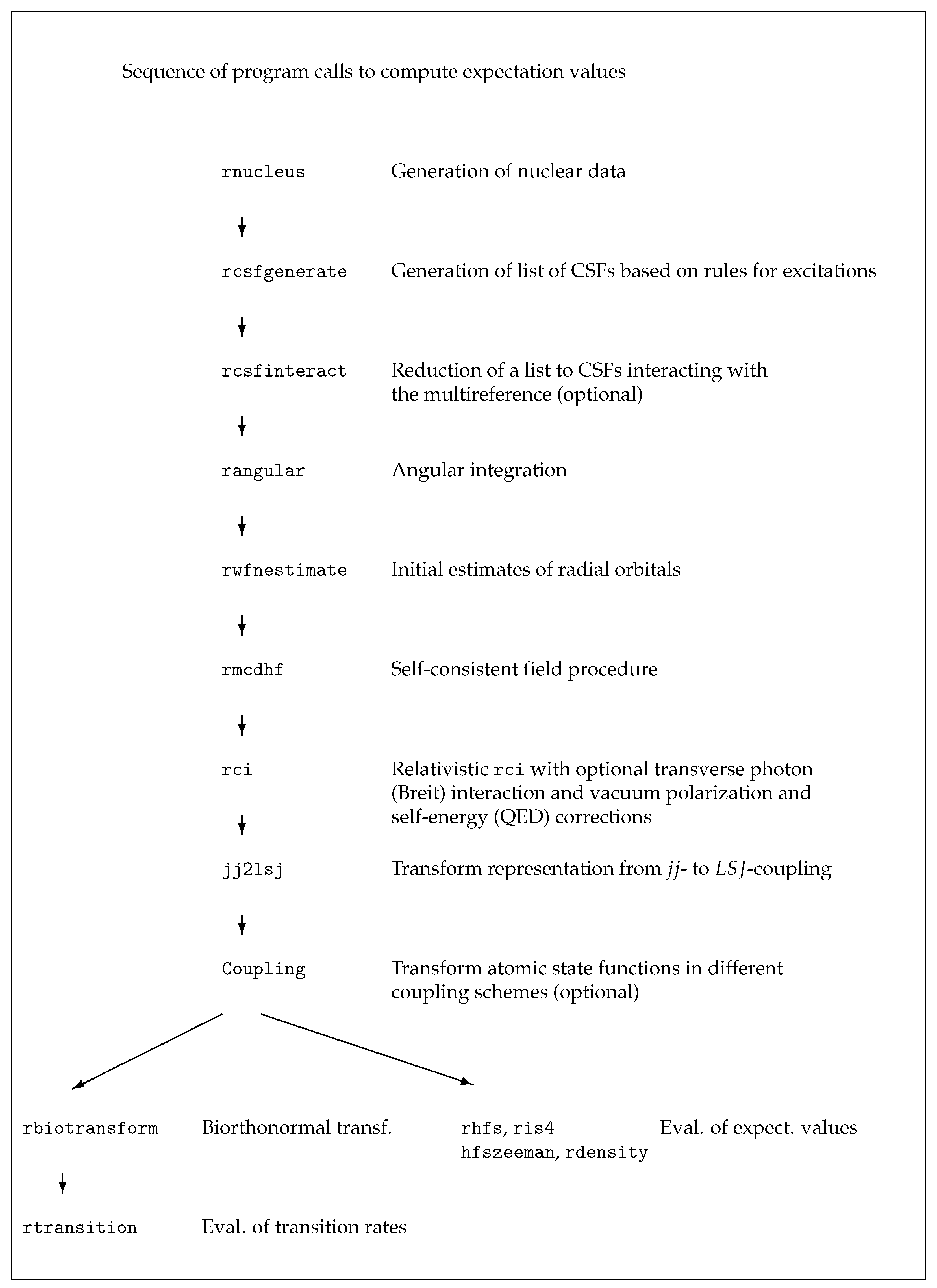
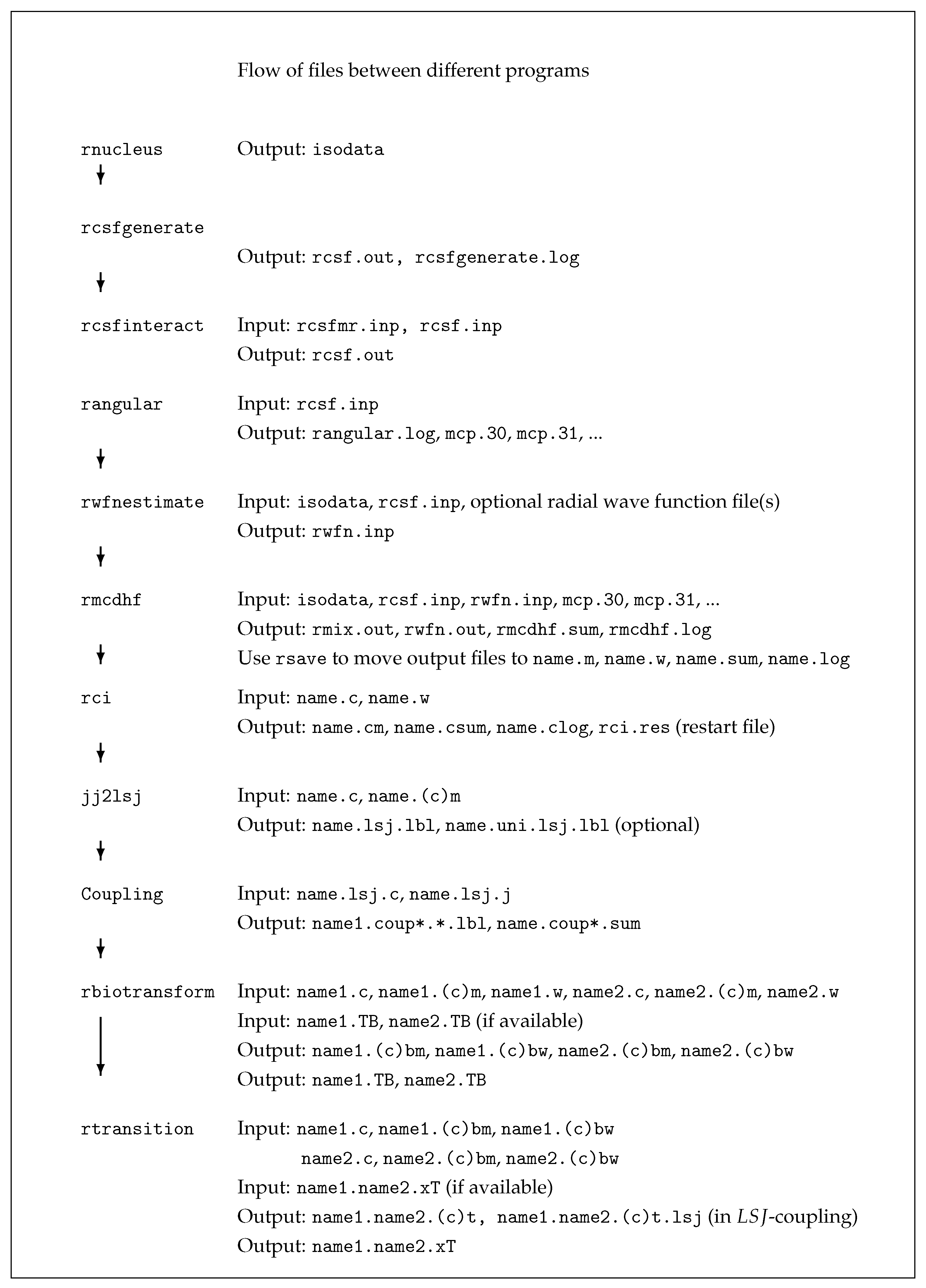
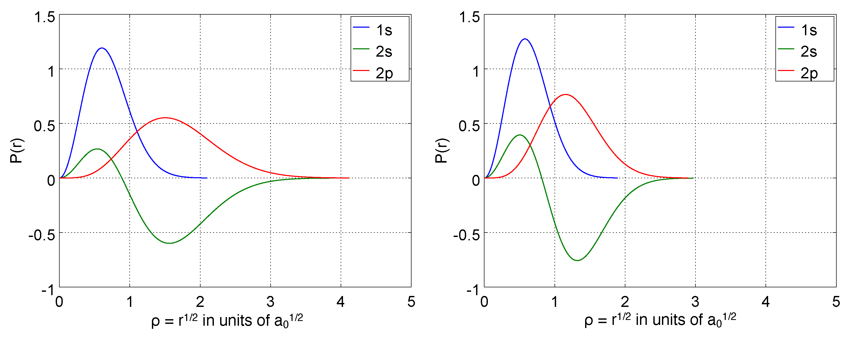
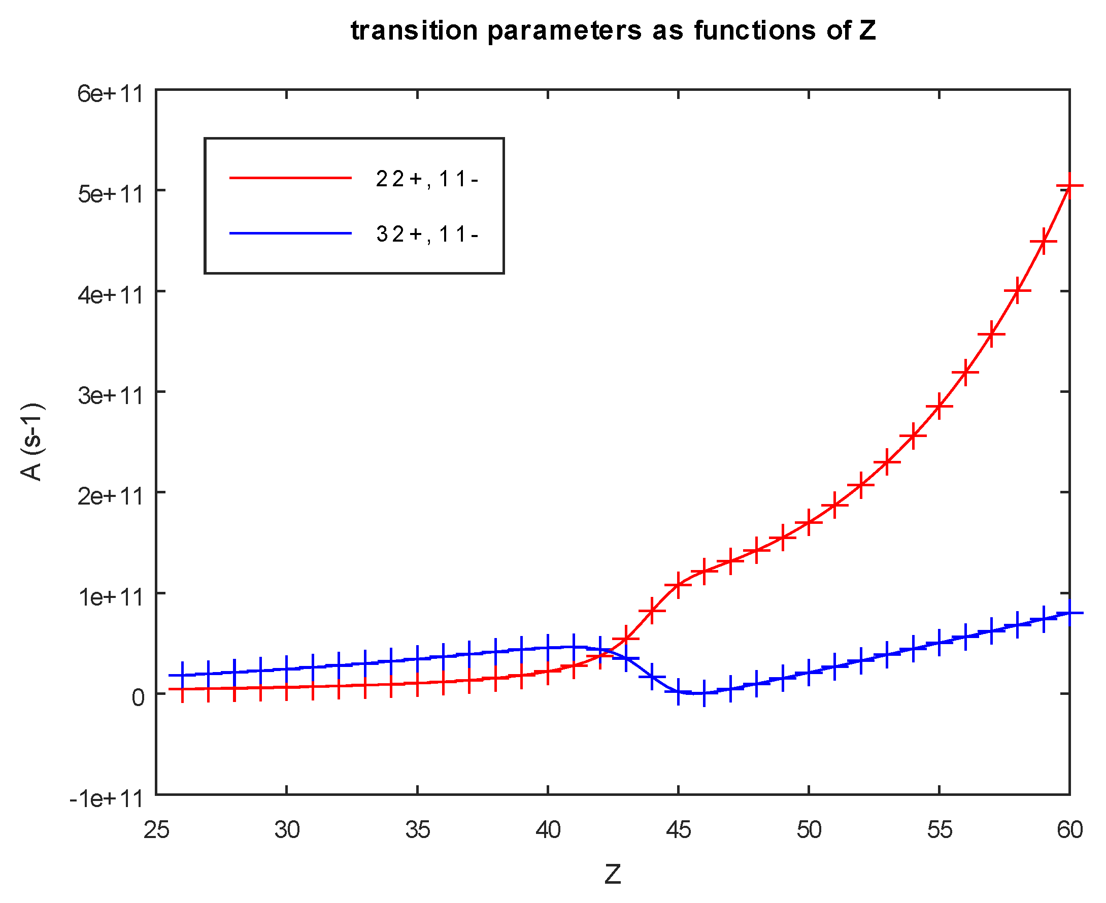
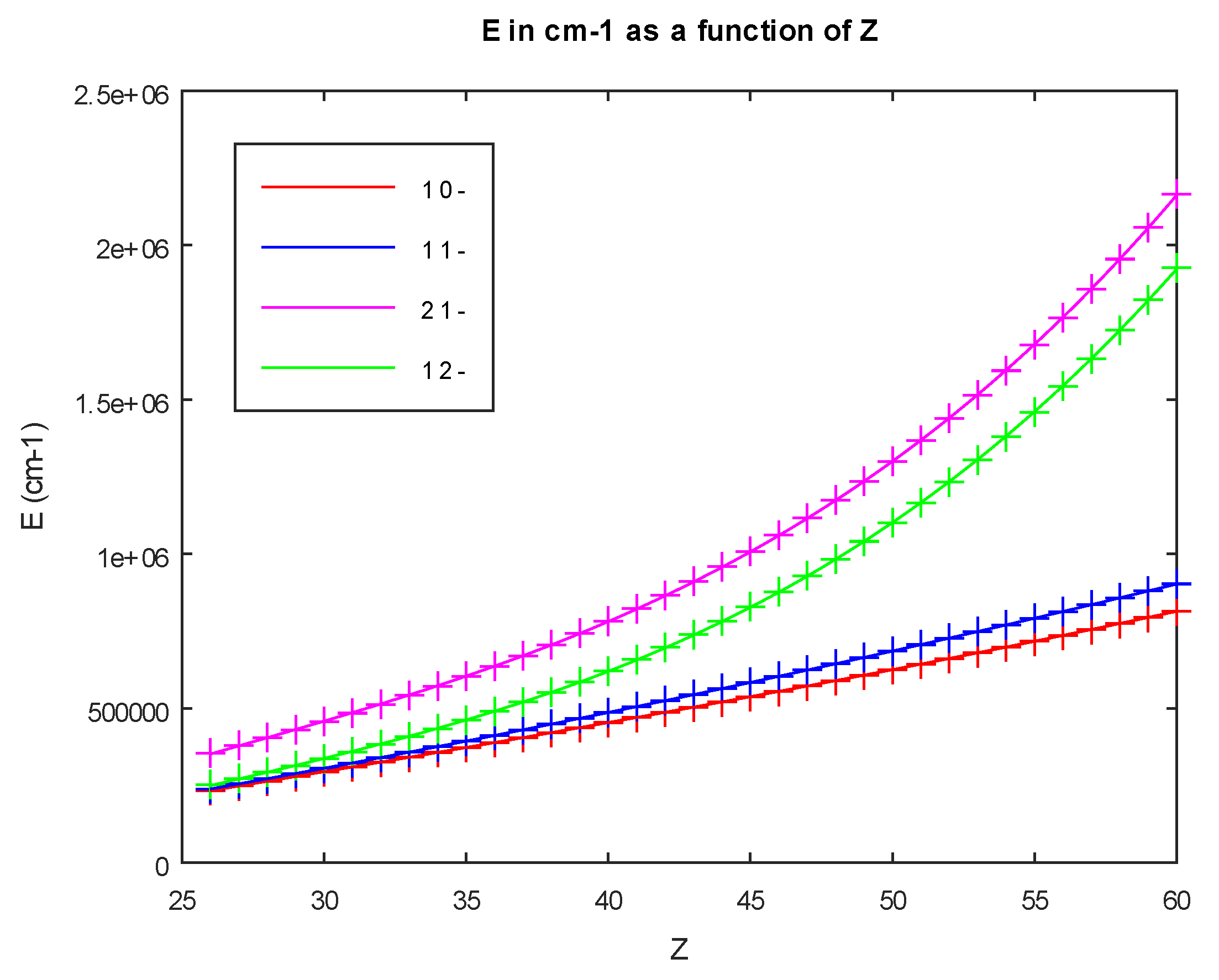
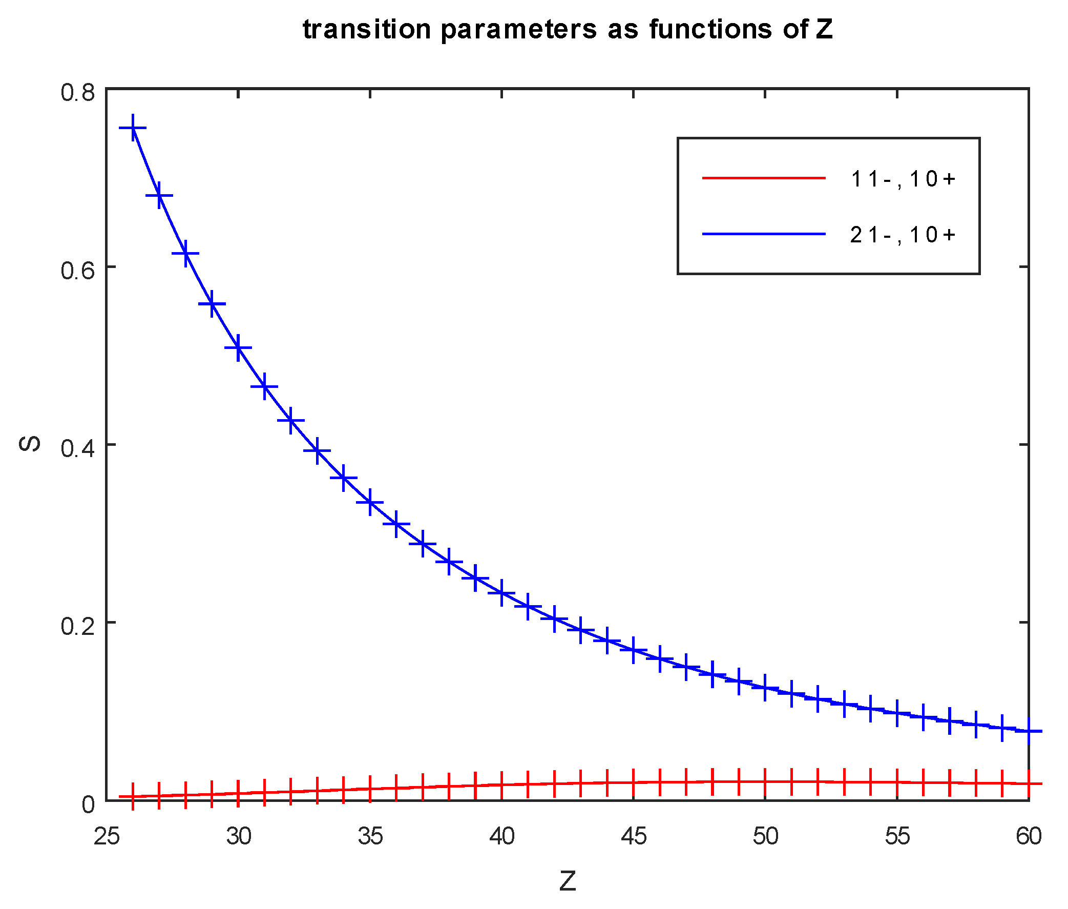
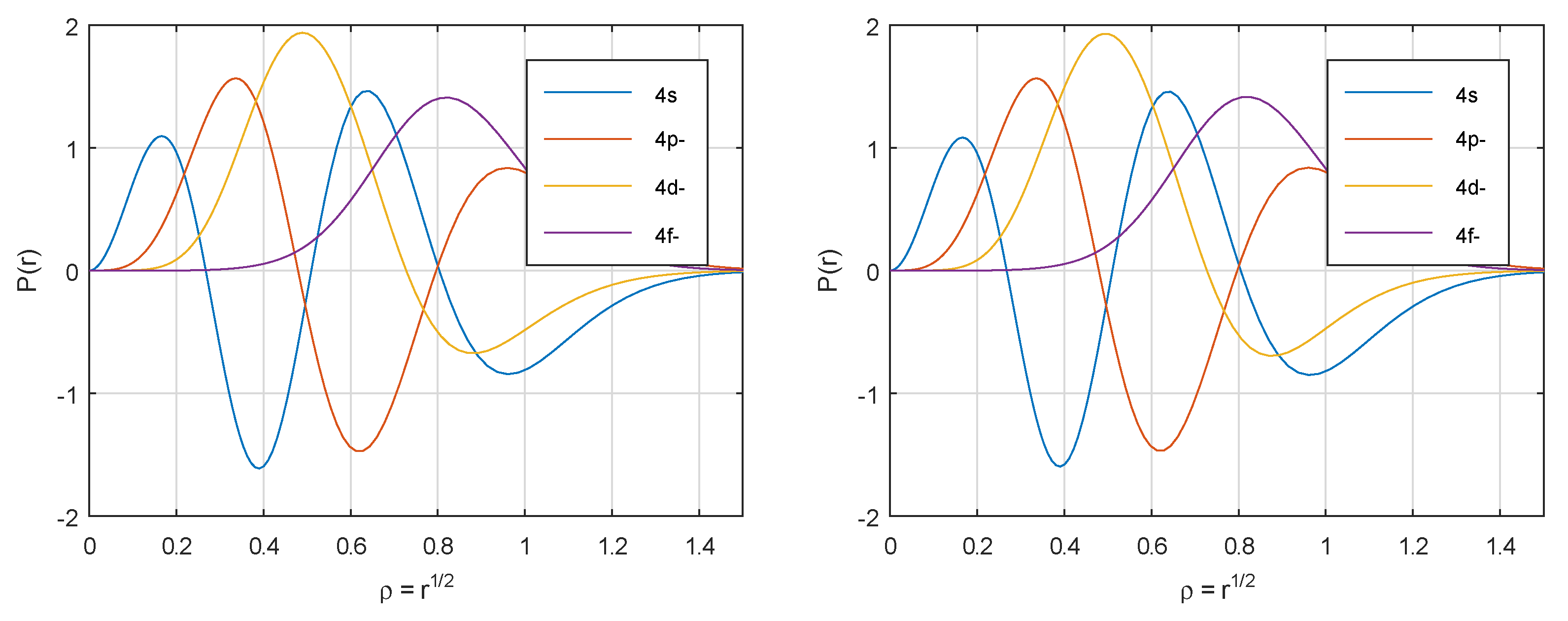9. Case Study I: $\mathbf{2}{\mathbf{s}}^{\mathbf{2}}\mathbf{2}\mathbf{p}$, $\mathbf{2}\mathbf{s}\mathbf{2}{\mathbf{p}}^{\mathbf{2}}$ in Mo XXXVIII Using Scripts

In this case study, we use script files to perform systematic calculations for all the states of the $2s^{2}2p$ and $2s2p^2$ configurations in Mo XXXVIII. The 10 states are as follows:

$$\mathrm{odd}:2s^{2}2p{}^2{P}_{1/2,3/2}^o$$

$$\mathrm{even}:2s2p^2{}^4{P}_{1/2,3/2,5/2},2s2p^2{}^2{D}_{3/2,5/2},2s2p^2{}^2{P}_{1/2,3/2},2s2p^2{}^2{S}_{1/2}$$

The script files can be found in grasptest/case1/script.

In a real application a correlation model should be defined, i.e., some rule to generate the CSFs from an orbital set. The convergence of computed properties is then monitored as the orbital set is increased. For the odd state, a reasonable correlation model is to start from the $\{1s^{2}2s^{2}2p,1s^{2}2p^3\}$ MR and then generate all CSFs that can be obtained by single and double excitations from the MR to an active set of orbitals. The active set of orbitals is then systematically increased. Following the normal conventions, the orbital set is denoted by the highest principal quantum number. For example, $n=3$ means the orbital set $\{1s,2s,2p,3s,3p,3d\}$. In this study, we increase the active set of orbitals up to $n=6$. For the even states, we start from the $1s^{2}2s2p^2$ reference and generate all CSFs that can be obtained by single and double excitations from the MR to the active sets of orbitals. The correlation model can be easily extended by adding CSFs to the MR.

9.1. Running Script Files

To automate the calculations, we use script files. For convenience, we have a main script that calls subscripts to perform different tasks. The construction of the scripts is greatly simplified if the names of the files are chosen in a simple and systematic way. In the case study we use the names odd2, odd3, odd4, odd5, odd6 and even2, even3, even4, even5, even6 to denote files for the odd and even parity states, respectively. The digit indicates which orbital set has been used to generate the expansion.

Before starting, please make sure that the grasp executables are on the path.

The main script sh_case1 is shown below. This script controls the computational flow and calls several subscripts.

#!/bin/sh
 
set -x
 
#    Main script for 2s(2)2p and 2s2p(2)
 
# 1.   Generate the expansions
        ./sh_files_c
 
# 2.   Get the nuclear data
        ./sh_nuc
 
# 3.   Get screened hydrogenic orbitals as initial estimates
        ./sh_initial
 
# 4.   Perform scf calculations and a final rci calculation that
#      includes the Breit correction and QED. All calculations
#      are transformed to LSJ-coupling. Files are created that
#      support creation of energy tables
        ./sh_scf
 
# 5.   Perform a transition calculation
        ./sh_tr

Each of the subscripts is given below together with some comments.

If all script files are available with execute permission (use the command chmod +x) we start the computation by typing the name of the main script

./sh_case1

Please note that these calculations will take several hours!

1.

Generate Expansions

The expansions are generated by the script sh_files_c. This is by far the most complicated script. It is simplified by generating lists for large active sets and then using rcsfsplit, see Section 7.1.

#!/bin/sh
 
set -x
 
#  1.  Generate CSF expansions
#      1.1 MR for 2s(2)2p, 2p(3)
 
rcsfgenerate <<OF1
*
0
1s(2,i)2s(2,i)2p(1,i)
1s(2,i)2p(3,i)
 
2s,2p
1,3
0
n
EOF1
 
cp rcsf.out odd2.c
 
#        1.2 SD-MR for n=6
 
rcsfgenerate <<EOF3
*
0
1s(2,*)2s(2,*)2p(1,*)
1s(2,*)2p(3,*)
 
6s,6p,6d,6f,6g,6h
1,3
2
n
EOF3
 
cp rcsf.out odd.c
 
#       Split into odd3.c, odd4.c, odd5.c, odd6.c
 
rcsfsplit <<EOF5
odd
4
3s,3p,3d
3
4s,4p,4d,4f
4
5s,5p,5d,5f,5g
5
6s,6p,6d,6f,6g,6h
6
EOF5
 
##########################################
 
#  2.  Generate CSF expansions
#      2.1 for 2s2p(2)
 
rcsfgenerate <<EOF1
*
0
1s(2,i)2s(1,i)2p(2,i)
 
2s,2p
1,5
0
n
EOF1
 
cp rcsf.out even2.c
 
#        2.2 SD for n=6
 
rcsfgenerate <<EOF3
*
0
1s(2,*)2s(1,*)2p(2,*)
6s,6p,6d,6f,6g,6h
1,5
2
n
EOF3
 
cp rcsf.out even.c
 
#        Split into even3.c, even4.c, even5.c, even6.c
 
rcsfsplit <<EOF5
even
4
3s,3p,3d
3
4s,4p,4d,4f
4
5s,5p,5d,5f,5g
5
6s,6p,6d,6f,6g,6h
6
EOF5

2.

Get Nuclear Data

Nuclear data are defined by the script sh_nuc. Since we are not interested in hyperfine structure, the nuclear spin and moments have all been set to 1.

#!/bin/sh
set -x
 
#  2.   Get nucleardata
rnucleus <<S1
42
96
n
96
1
1
1
S1
 
cat isodata

3.

Get Initial Estimates

The script sh_initial performs angular integration, gets initial estimates and performs rmcdhf calculations for the odd and even reference states (odd2 and even2). As initial estimates, we use screened hydrogenic functions. For the reference states, all orbitals are required to be spectroscopic, i.e., they should have the correct number of nodes, see Section 7.1

#!/bin/sh
set -x
 
# 3. For n=2, Get initial estimates for odd.
 
cp odd2.c rcsf.inp
rangular  <<S4
y
S4
 
#  Get initial estimates of wave functions
rwfnestimate <<S5
y
3
*
S5
 
# Perform self-consistent field calculations
rmcdhf > outodd_rmcdhf_initial <<S6
y
1
1
5
*
*
100
S6
 
#  Save the result to odd2
rsave odd2
 
# 3. For n=2, Get initial estimates for even
 
cp even2.c rcsf.inp
rangular  <<S4
y
S4
 
#  Get initial estimates of wave functions
rwfnestimate <<S5
y
3
*
S5
 
# Perform self-consistent field calculations
rmcdhf > outeven_rmcdhf_initial <<S6
y
1,2,3
1,2,3
1,2
5
*
*
100
S6
 
#  Save the result to even2
rsave even2

4.

rmcdhf and rci Calculations

The script sh_scf performs angular integration, estimates the new radial functions and performs rmcdhf for the odd and even states up to $n=6$. At the end, rci calculations are performed for the largest expansions. The rci calculations include Breit interaction and QED corrections. All results are transformed to $LSJ$-coupling. Please note how we loop in the script over the digit n that indicates the size of the orbital set.

#!/bin/sh
set -x
 
#   4.  Get results for odd n=3,4,5,6
 
for n in 3 4 5 6
do
   (cp odd${n}.c rcsf.inp
 
#  Get angular data
rangular <<S4
y
S4
 
# Get initial estimates of wave functions
m=`expr $n - 1`
echo m=$m n=$n
rwfnestimate <<S5
y
1
odd${m}.w
*
3
*
S5
 
# Perform self-consistent field calculations
rmcdhf > outodd_rmcdhf_${n} <<S6
y
1
1
5
${n}*
 
100
S6
 
rsave odd${n}
 
# transform to LSJ-coupling
 
jj2lsj  <<S1
odd${n}
n
y
y
S1
 
   echo)
done
 
#  Perform Breit-correction using RCI for n=6. First copy to other file names
 
n=6
cp odd${n}.c oddCI${n}.c
cp odd${n}.w oddCI${n}.w
 
rci > outodd_rci <<S7
y
oddCI${n}
y
y
1.d-6
y
n
n
y
4
1
1
S7
 
# transform to LSJ-coupling
 
jj2lsj  <<S1
oddCI${n}
y
y
y
S1
 
 
#   4.  Get results for even n=3,4,5,6
 
for n in 3 4 5 6
do
   (cp even${n}.c rcsf.inp
 
#  Get angular data
rangular <<S4
y
S4
 
# Get initial estimates of wave functions
m=`expr $n - 1`
echo m=$m n=$n
rwfnestimate <<S5
y
1
even${m}.w
*
3
*
S5
 
# Perform self-consistent field calculations
rmcdhf > outeven_rmcdhf_${n} <<S6
y
1,2,3
1,2,3
1,2
5
${n}*
 
100
S6
 
rsave even${n}
 
# transform to LSJ-coupling
 
jj2lsj  <<S1
even${n}
n
y
y
S1
 
 
   echo)
done
 
#  Perform Breit-correction using RCI for n=6
 
n=6
cp even${n}.c evenCI${n}.c
cp even${n}.w evenCI${n}.w
 
rci > outeven_rci <<S7
y
evenCI${n}
y
y
1.d-6
y
n
n
y
4
1,2,3
1,2,3
1,2
S7
 
# transform to LSJ-coupling
 
jj2lsj  <<S1
evenCI${n}
y
y
y
S1

5.

Transition calculation

The script sh_tr computes the E1 transition rates between the odd and even states. First we perform a biorthonormal transformation, and then we perform the transition calculation itself.

#!/bin/sh
set -x
 
#  6. Perform transition calculation for the n=6 CI results
 
n=6
 
#  First the biorthonormal transformations
 
rbiotransform > out_rbiotransform <<EOF
y
y
oddCI$n
evenCI$n
y
EOF
 
# Then the transition calculations
 
rtransition > out_transition <<EOF
y
y
oddCI$n
evenCI$n
E1
EOF

9.2. Comparison with Experiment

To display the computed energies we give the command

rlevels oddCI6.cm evenCI6.cm

The computer returns the energies together with labels in $LSJ$-coupling for all the states.

 nblock =            2   ncftot =        20641   nw =           36   nelec =            5
 nblock =            3   ncftot =        36290   nw =           36   nelec =            5
 
 Energy levels for ...
 Rydberg constant is   109737.31569
 Splitting is the energy difference with the lower neighbor
------------------------------------------------------------------------------------------
 No Pos  J Parity Energy Total    Levels     Splitting     Configuration
                      (a.u.)      (cm^-1)     (cm^-1)
------------------------------------------------------------------------------------------
  1  1  1/2 -   -2386.3200262        0.00        0.00  1s(2).2s(2).2p_2P
  2  1  1/2 +   -2382.2391997   895637.89   895637.89  1s(2).2s_2S.2p(2)3P2_4P
  3  1  3/2 -   -2381.9242100   964770.13    69132.25  1s(2).2s(2).2p_2P
  4  1  3/2 +   -2378.9986341  1606859.82   642089.69  1s(2).2s_2S.2p(2)3P2_4P
  5  1  5/2 +   -2378.1476302  1793633.59   186773.77  1s(2).2s_2S.2p(2)3P2_4P
  6  2  3/2 +   -2376.7269966  2105426.64   311793.05  1s(2).2s_2S.2p(2)1D2_2D
  7  2  1/2 +   -2376.5312708  2148383.48    42956.84  1s(2).2s_2S.2p(2)3P2_2P
  8  2  5/2 +   -2373.9013617  2725581.82   577198.34  1s(2).2s_2S.2p(2)1D2_2D
  9  3  1/2 +   -2371.9005560  3164707.90   439126.08  1s(2).2s_2S.2p(2)1S0_2S
 10  3  3/2 +   -2371.8561115  3174462.35     9754.45  1s(2).2s_2S.2p(2)3P2_2P
------------------------------------------------------------------------------------------

The Mo XXXVIII transitions have been observed in the JET Tokamak, Myrnäs et al. [44]. In the Table 8, the experimental transition energies are compared with the calculated energies. Please note that the quantum labels for the $2s2p^2{}^2{P}_{1/2}$ and $2s2p^2{}^2{S}_{1/2}$ seem to have been swapped in the experimental paper, i.e., the highest $J=1/2$ state should be $2s2p^2{}^2{S}_{1/2}$ and not $2s2p^2{}^2{P}_{1/2}$. We see that the odd states are somewhat too high. This is due to an imbalance in the MR. As discussed in the beginning of the section the correlation model can be refined by extending the MR. Adopting the MRs $\{2s^{2}2p,2p^3,2s2p3d,2p^{2}3d\}$ and $\{2s2p^2,2p^{2}3d,2s^{2}3d,2s3d^2\}$ for, respectively, the odd and even parity states improves the energy separations considerably [45]. A careful investigation of the effects of increasing the MR is part of any systematic calculation (see Section 6.6).

Table 8. Experimental and computed excitation energies for Mo XXXVIII.

State (Exp. Label)	$\Delta {\mathit{E}}^{\mathit{a}}$ (cm${}^{-1}$)	$\Delta {\mathit{E}}^{\mathit{b}}$ (cm${}^{-1}$)
$2s^{2}2p{}^2{P}_{1/2}^o$	0	0
$2s2p^2{}^4{P}_{1/2}$	894 050 $\pm 400$	895 848
$2s^{2}2p{}^2{P}_{3/2}^o$	964 050 $\pm 90$	964 715
$2s2p^2{}^4{P}_{3/2}$		1 606 863
$2s2p^2{}^4{P}_{5/2}$	1 790 130 $\pm 200$	1 793 682
$2s2p^2{}^2{D}_{3/2}$	2 102 900 $\pm 900$	2 106 354
$2s2p^2{}^2{S}_{1/2}$	2 147 300 $\pm 900$	2 149 456
$2s2p^2{}^2{D}_{5/2}$		2 725 586
$2s2p^2{}^2{P}_{1/2}$	3 164 770 $\pm 1500$	3 166 168
$2s2p^2{}^2{P}_{3/2}$	3 171 300 $\pm 1500$	3 175 559

^a Exp. (Myrnäs et al., [44]), ^b Calc. (Rynkun et al. [45]).

9.3. Transition Rates

Below are the transition parameters as given in the file oddCI6.evenCI6.ct.lsj. The agreement between calculated values in the two gauges (the first line gives values in length gauge and the second line gives values in velocity gauge) is quite good, especially for the strong transitions. Expansions based on a larger MR set will further improve the agreement. The quantity $dT$ is defined as

$$dT=\frac{|A_C-A_B|}{max(A_C,A_B)},$$

where $A_B$ and $A_C$ are the transition rates in length and velocity gauge. $dT$ is a measure of the uncertainty of the computed transition rates [43].

 Transition between files:
 oddCI6
 evenCI6
 
  
   1-2386.32002619  1s(2).2s(2).2p_2P
   1-2382.23919972  1s(2).2s_2S.2p(2)3P2_4P
  895637.89 CM-1       111.65 ANGS(VAC)       111.65 ANGS(AIR)
 E1  S =  4.42135D-03   GF =  1.20285D-02   AKI =  3.21802D+09   dT =  0.05152
          4.66152D-03         1.26819D-02          3.39282D+09
 
  
   1-2386.32002619  1s(2).2s(2).2p_2P
   1-2376.53127082  1s(2).2s_2S.2p(2)3P2_2P
 2148383.48 CM-1        46.55 ANGS(VAC)        46.55 ANGS(AIR)
 E1  S =  1.87910D-02   GF =  1.22627D-01   AKI =  1.88765D+11   dT =  0.00415
          1.88692D-02         1.23137D-01          1.89551D+11
 
  
   1-2386.32002619  1s(2).2s(2).2p_2P
   1-2371.90055603  1s(2).2s_2S.2p(2)1S0_2S
 3164707.90 CM-1        31.60 ANGS(VAC)        31.60 ANGS(AIR)
 E1  S =  1.51571D-05   GF =  1.45705D-04   AKI =  4.86690D+08   dT =  0.06893
          1.62792D-05         1.56492D-04          5.22723D+08
  
  
   1-2386.32002619  1s(2).2s(2).2p_2P
   3-2378.99863414  1s(2).2s_2S.2p(2)3P2_4P
 1606859.82 CM-1        62.23 ANGS(VAC)        62.23 ANGS(AIR)
 E1  S =  1.11563D-04   GF =  5.44533D-04   AKI =  2.34457D+08   dT =  0.01690
          1.13481D-04         5.53892D-04          2.38486D+08
 
 
   1-2386.32002619  1s(2).2s(2).2p_2P
   3-2376.72699656  1s(2).2s_2S.2p(2)1D2_2D
 2105426.64 CM-1        47.50 ANGS(VAC)        47.50 ANGS(AIR)
 E1  S =  2.45759D-02   GF =  1.57172D-01   AKI =  1.16181D+11   dT =  0.00644
          2.47352D-02         1.58190D-01          1.16934D+11
 
 
   1-2386.32002619  1s(2).2s(2).2p_2P
   3-2371.85611149  1s(2).2s_2S.2p(2)3P2_2P
 3174462.35 CM-1        31.50 ANGS(VAC)        31.50 ANGS(AIR)
 E1  S =  6.34294D-04   GF =  6.11625D-03   AKI =  1.02780D+10   dT =  0.00529
          6.30940D-04         6.08391D-03          1.02236D+10
  
  
   1-2382.23919972  1s(2).2s_2S.2p(2)3P2_4P
   3-2381.92421002  1s(2).2s(2).2p_2P
   69132.25 CM-1      1446.50 ANGS(VAC)      1446.50 ANGS(AIR)
 E1  S =  5.06265D-04   GF =  1.06312D-04   AKI =  8.47280D+04   dT =  0.18843
          4.10869D-04         8.62797D-05          6.87626D+04
 
  
   3-2381.92421002  1s(2).2s(2).2p_2P
   1-2376.53127082  1s(2).2s_2S.2p(2)3P2_2P
 1183613.34 CM-1        84.49 ANGS(VAC)        84.49 ANGS(AIR)
 E1  S =  2.36464D-03   GF =  8.50157D-03   AKI =  3.97220D+09   dT =  0.05227
          2.49506D-03         8.97046D-03          4.19128D+09
 
  
   3-2381.92421002  1s(2).2s(2).2p_2P
   1-2371.90055603  1s(2).2s_2S.2p(2)1S0_2S
 2199937.76 CM-1        45.46 ANGS(VAC)        45.46 ANGS(AIR)
 E1  S =  1.48021D-02   GF =  9.89140D-02   AKI =  1.59658D+11   dT =  0.00260
          1.47636D-02         9.86566D-02          1.59243D+11
 
  
   3-2381.92421002  1s(2).2s(2).2p_2P
   3-2378.99863414  1s(2).2s_2S.2p(2)3P2_4P
  642089.69 CM-1       155.74 ANGS(VAC)       155.74 ANGS(AIR)
 E1  S =  1.00858D-03   GF =  1.96712D-03   AKI =  1.35240D+08   dT =  0.11531
          1.14004D-03         2.22352D-03          1.52867D+08
 
  
   3-2381.92421002  1s(2).2s(2).2p_2P
   3-2376.72699656  1s(2).2s_2S.2p(2)1D2_2D
 1140656.51 CM-1        87.67 ANGS(VAC)        87.67 ANGS(AIR)
 E1  S =  2.73257D-03   GF =  9.46784D-03   AKI =  2.05420D+09   dT =  0.04984
          2.87592D-03         9.96450D-03          2.16196D+09
 
  
   3-2381.92421002  1s(2).2s(2).2p_2P
   3-2371.85611149  1s(2).2s_2S.2p(2)3P2_2P
 2209692.21 CM-1        45.26 ANGS(VAC)        45.26 ANGS(AIR)
 E1  S =  4.49452D-02   GF =  3.01675D-01   AKI =  2.45632D+11   dT =  0.00389
          4.51208D-02         3.02854D-01          2.46592D+11
 
  
   3-2381.92421002  1s(2).2s(2).2p_2P
   5-2378.14763025  1s(2).2s_2S.2p(2)3P2_4P
  828863.45 CM-1       120.65 ANGS(VAC)       120.65 ANGS(AIR)
 E1  S =  9.97378D-03   GF =  2.51112D-02   AKI =  1.91789D+09   dT =  0.08159
          1.08599D-02         2.73422D-02          2.08828D+09
 
 
   3-2381.92421002  1s(2).2s(2).2p_2P
   5-2373.90136166  1s(2).2s_2S.2p(2)1D2_2D
 1760811.69 CM-1        56.79 ANGS(VAC)        56.79 ANGS(AIR)
 E1  S =  1.52580D-02   GF =  8.16083D-02   AKI =  2.81288D+10   dT =  0.01679
          1.55185D-02         8.30017D-02          2.86091D+10

9.4. LaTeX Table with Energies as Functions of the Active Set

The script sh_scf is written in such a way that all results are transformed to $LSJ$-coupling using jj2lsj. The output from rlevels will then contain quantum labels of the states in $LSJ$-coupling. By saving the output from rlevels we can generate a LaTeX table showing the convergence of the energies as the active set is increased. If we include also the output from the final rci calculation, we can see the effect of the Breit interaction and QED.

Issuing the commands below saves the output from rlevels corresponding to the increasing active set of orbitals in files energy3, energy4, energy5, energy6, energyCI6

>>rlevels even3.m odd3.m > energy3
>>rlevels even4.m odd4.m > energy4
>>rlevels even5.m odd5.m > energy5
>>rlevels even6.m odd6.m > energy6
>>rlevels evenCI6.cm oddCI6.cm > energyCI6

We now call rtablevels to produce a LaTeX table, see Section 7.6

>>rtablevels
 
 RTABLEVELS
 Makes LaTeX and ASCII tables of energy files produced by
 rlevels (in ljs format)
 Multiple energy files can be used as input
 Energies from file 1 fills column 1, energies from file 2
 fills column 2 etc.  Checks are done to see if the labels
 if the labels in the files are consistent
 Input file: name1, name2, ...
 Output files: energylabellatex.tex, energylabelascii.txt
 
 Inspect energy files and determine how many positions
 should be skipped in the string that determines the label
 e.g., if the string is 1s(2).2s_2S.2p(2)3P2_4P and 1s(2) is a core
 then you would like to skip 1s(2). i.e., 6 positions and determine
 the label from 2s_2S.2p(2)3P2_4P
 
 How many positions should be skipped?
>>6
 Give the number of energy files from rlevels
>>5
 Name of file 1
>>energy3
 Name of file 2
>>energy4
 Name of file 3
>>energy5
 Name of file 4
>>energy6
 Name of file 5
>>energyCI6

The generated LaTeX table is named energytablelatex.tex. After processing we obtain Table 9.

Table 9. Energies in cm${}^{-1}$ from the files energy3, energy4, energy5, energy6, energyCI6.

$2s^{2}2p{}^2{P}_{1/2}^o$	0	0	0	0	0
$2s{}^{2}S2p^2{(}_2^{3}P){}^4{P}_{1/2}$	894248	894018	893855	893920	895637
$2s^{2}2p{}^2{P}_{3/2}^o$	982556	982796	982807	982793	964770
$2s{}^{2}S2p^2{(}_2^{3}P){}^4{P}_{3/2}$	1620240	1621107	1621267	1621540	1606859
$2s{}^{2}S2p^2{(}_2^{3}P){}^4{P}_{5/2}$	1823232	1823052	1822927	1823033	1793633
$2s{}^{2}S2p^2{(}_2^{1}D){}^2{D}_{3/2}$	2130522	2128609	2128002	2127792	2105426
$2s{}^{2}S2p^2{(}_2^{3}P){}^2{P}_{1/2}$	2163550	2161641	2160998	2160705	2148383
$2s{}^{2}S2p^2{(}_2^{1}D){}^2{D}_{5/2}$	2764810	2764403	2764217	2764261	2725581
$2s{}^{2}S2p^2{(}_0^{1}S){}^2{S}_{1/2}$	3193694	3191337	3190537	3190063	3164707
$2s{}^{2}S2p^2{(}_2^{3}P){}^2{P}_{3/2}$	3213578	3211491	3210805	3210469	3174462

From the table, we see that the energies seem to be reasonably converged when the active orbital set has been increased to $n=6$. We also see that the Breit interaction and QED, as included in the final rci calculation, change the energies substantially.

At this point, it is appropriate to comment on the labels. The $LS$ term for electrons with occupation one is not written out. The $LS$ terms for equivalent electrons with occupation two or more are written in parentheses together with the seniority number. The angular momenta are coupled from left to right and written in a linear fashion. As an example, we look at

$$2s{}^{2}S2p^2{(}_2^{3}P){}^4{P}_{5/2}$$

The $2s$ electron has the $LS$ term ${}^{2}S$, but this is not written out explicitly. The $2p^2$ has the $LS$ term ${}^{3}P$ with seniority 2. This is written as $2p^2{(}_2^{3}P)$. Coupling the ${}^{1}S$ term of the $1s^2$ core (not included in the label) with the ${}^{2}S$ term of $2s$ results in ${}^{2}S$. The ${}^{2}S$ term in turn is coupled with the ${}^{3}P$ term to yield ${}^{4}P$. The final L and S are then coupled to $J=5/2$. See also section 9.2 for a more detailed account of the labels.

9.5. LaTeX Table with Transition Data

There is also a program rtabtransE1, see Section 7.7, that produces a transition file. There are different options for the table. Below, we choose to display $gf$ and A in the length gauge together with $dT$

>>rtabtransE1
 
 RTABTRANSE1
 Makes LaTeX tables of transition data from transition files
 name1.name2.ct.lsj
 Input file: name1.name2.ct.lsj
 Output file: transitiontable.tex
 
 Specify table format
 (1). Lower & Upper & Energy diff. & wavelength & S & gf & A & dT
 (2). Lower & Upper & Energy diff. & wavelength & gf & A & dT
 (3). Lower & Upper & Energy diff. & wavelength & gf & A
 (4). Lower & Upper & Energy diff. & S & gf & A & dT
 (5). Lower & Upper & Energy diff. & gf & A & dT
 (6). Lower & Upper & Energy diff. & gf & A
>>5
 Inspect the name1.name2.ct.lsj file and determine how many positions
 should be skipped in the string that determines the label
 e.g., if the string is 1s(2).2s_2S.2p(2)3P2_4P and 1s(2) is a core
 then you would like to skip 1s(2). i.e., 6 positions and determine
 the label from 2s_2S.2p(2)3P2_4P
 
 How many positions should be skipped?
>>6
Name of file
>>oddCI6.evenCI6.ct.lsj

The generated LaTeX table is named transitiontable.tex. After processing we obtain Table 10.

Table 10. Transition data from the file oddCI6.evenCI6.ct.lsj.

Lower State	Upper State	$\Delta \mathit{E}$ (cm${}^{-1}$)	$\mathit{g}\mathit{f}$	A (s${}^{-1}$)	$\mathit{d}\mathit{T}$
$2s^{2}2p{}^2{P}_{1/2}$	$2s{}^{2}S2p^2{(}_2^{3}P){}^4{P}_{1/2}$	895637	1.202D-02	3.218D+09	0.051
$2s^{2}2p{}^2{P}_{1/2}$	$2s{}^{2}S2p^2{(}_2^{3}P){}^2{P}_{1/2}$	2148383	1.226D-01	1.887D+11	0.004
$2s^{2}2p{}^2{P}_{1/2}$	$2s{}^{2}S2p^2{(}_0^{1}S){}^2{S}_{1/2}$	3164707	1.457D-04	4.866D+08	0.068
$2s^{2}2p{}^2{P}_{1/2}$	$2s{}^{2}S2p^2{(}_2^{3}P){}^4{P}_{3/2}$	1606859	5.445D-04	2.344D+08	0.016
$2s^{2}2p{}^2{P}_{1/2}$	$2s{}^{2}S2p^2{(}_2^{1}D){}^2{D}_{3/2}$	2105426	1.571D-01	1.161D+11	0.006
$2s^{2}2p{}^2{P}_{1/2}$	$2s{}^{2}S2p^2{(}_2^{3}P){}^2{P}_{3/2}$	3174462	6.116D-03	1.027D+10	0.005
$2s{}^{2}S2p^2{(}_2^{3}P){}^4{P}_{1/2}$	$2s^{2}2p{}^2{P}_{3/2}$	69132	1.063D-04	8.472D+04	0.188
$2s^{2}2p{}^2{P}_{3/2}$	$2s{}^{2}S2p^2{(}_2^{3}P){}^2{P}_{1/2}$	1183613	8.501D-03	3.972D+09	0.052
$2s^{2}2p{}^2{P}_{3/2}$	$2s{}^{2}S2p^2{(}_0^{1}S){}^2{S}_{1/2}$	2199937	9.891D-02	1.596D+11	0.002
$2s^{2}2p{}^2{P}_{3/2}$	$2s{}^{2}S2p^2{(}_2^{3}P){}^4{P}_{3/2}$	642089	1.967D-03	1.352D+08	0.115
$2s^{2}2p{}^2{P}_{3/2}$	$2s{}^{2}S2p^2{(}_2^{1}D){}^2{D}_{3/2}$	1140656	9.467D-03	2.054D+09	0.049
$2s^{2}2p{}^2{P}_{3/2}$	$2s{}^{2}S2p^2{(}_2^{3}P){}^2{P}_{3/2}$	2209692	3.016D-01	2.456D+11	0.003
$2s^{2}2p{}^2{P}_{3/2}$	$2s{}^{2}S2p^2{(}_2^{3}P){}^4{P}_{5/2}$	828863	2.511D-02	1.917D+09	0.081
$2s^{2}2p{}^2{P}_{3/2}$	$2s{}^{2}S2p^2{(}_2^{1}D){}^2{D}_{5/2}$	1760811	8.160D-02	2.812D+10	0.016

9.6. Editing the LaTeX Table

The table programs translate the $LSJ$-notation from jj2lsj to LaTeX notation. If the user wants to simplify or change the LaTeX notation, this is easily done. For example, the global substitution 2s~^2\!S\, → 2s in the LaTeX file produces Table 11.

Table 11. Transition data from the file oddCI6.evenCI6.ct.lsj.

Lower State	Upper State	$\Delta \mathit{E}$ (cm${}^{-1}$)	$\mathit{g}\mathit{f}$	A (s${}^{-1}$)	$\mathit{d}\mathit{T}$
$2s^{2}2p{}^2{P}_{1/2}$	$2s2p^2{(}_2^{3}P){}^4{P}_{1/2}$	895637	1.202D-02	3.218D+09	0.051
$2s^{2}2p{}^2{P}_{1/2}$	$2s2p^2{(}_2^{3}P){}^2{P}_{1/2}$	2148383	1.226D-01	1.887D+11	0.004
$2s^{2}2p{}^2{P}_{1/2}$	$2s2p^2{(}_0^{1}S){}^2{S}_{1/2}$	3164707	1.457D-04	4.866D+08	0.068
$2s^{2}2p{}^2{P}_{1/2}$	$2s2p^2{(}_2^{3}P){}^4{P}_{3/2}$	1606859	5.445D-04	2.344D+08	0.016
$2s^{2}2p{}^2{P}_{1/2}$	$2s2p^2{(}_2^{1}D){}^2{D}_{3/2}$	2105426	1.571D-01	1.161D+11	0.006
$2s^{2}2p{}^2{P}_{1/2}$	$2s2p^2{(}_2^{3}P){}^2{P}_{3/2}$	3174462	6.116D-03	1.027D+10	0.005
$2s2p^2{(}_2^{3}P){}^4{P}_{1/2}$	$2s^{2}2p{}^2{P}_{3/2}$	69132	1.063D-04	8.472D+04	0.188
$2s^{2}2p{}^2{P}_{3/2}$	$2s2p^2{(}_2^{3}P){}^2{P}_{1/2}$	1183613	8.501D-03	3.972D+09	0.052
$2s^{2}2p{}^2{P}_{3/2}$	$2s2p^2{(}_0^{1}S){}^2{S}_{1/2}$	2199937	9.891D-02	1.596D+11	0.002
$2s^{2}2p{}^2{P}_{3/2}$	$2s2p^2{(}_2^{3}P){}^4{P}_{3/2}$	642089	1.967D-03	1.352D+08	0.115
$2s^{2}2p{}^2{P}_{3/2}$	$2s2p^2{(}_2^{1}D){}^2{D}_{3/2}$	1140656	9.467D-03	2.054D+09	0.049
$2s^{2}2p{}^2{P}_{3/2}$	$2s2p^2{(}_2^{3}P){}^2{P}_{3/2}$	2209692	3.016D-01	2.456D+11	0.003
$2s^{2}2p{}^2{P}_{3/2}$	$2s2p^2{(}_2^{3}P){}^4{P}_{5/2}$	828863	2.511D-02	1.917D+09	0.081
$2s^{2}2p{}^2{P}_{3/2}$	$2s2p^2{(}_2^{1}D){}^2{D}_{5/2}$	1760811	8.160D-02	2.812D+10	0.016

9.7. Scripts for MPI Codes

The scripts above can, with very small modifications, also be used for performing the runs using the MPI codes. Before running the scripts for the MPI code, the file disks with paths to the working directory and to the directory containing temporary data must be created, see Section 6.4. In the different scripts, the calls to the MPI programs amount to changes of the type

     rangular   -->  mpirun -np 8 rangular_mpi
 
     rmcdhf     -->  mpirun -np 8 rmcdhf_mpi
 
     rci        -->  mpirun -np 8 rci_mpi

etc. Scripts for the MPI cases are included under case1_mpi in the test data set. Consult the README file in the working directory for more details on setting up the file disks.

10. Case Study II: The Li Iso-Electronic Sequence Using Scripts

In this case study, we use script files to perform systematic calculations for the $1s^{2}2s{}^2{S}_{1/2}$ ground state and the $1s^{2}2p{}^2{P}_{1/2,3/2}^o$ excited states in the Li iso-electronic sequence. Computing data for an iso-electronic sequence, angular data can be reused and need not be recomputed for each member of the sequence. The script files can be found in grasptest/case2/script.

We start with a single calculation of the three reference states. After that, separate calculations are done for the two parities. Correlation is then included by allowing single, double, and triple (SDT) excitations from the reference to active sets up to $n=5$ (complete active space calculations). Calculations including hyperfine structures and transition rates are performed from $Z=6$ to $Z=12$.

It is convenient to save the results for the different ions in directories Z6, Z7, Z8, …, Z12.

10.1. Running Script Files

The main script sh_case2 is shown below. This script controls the computational flow and calls several subscripts.

#!/bin/sh
 
set -x
 
#    Main script for iso-electronic sequence
 
# 1.   Generate directories Z6, Z7, .. for the elements
#      Define nuclear data for each element
 
        ./sh_nuc_seq
 
# 2.   Generate lists of CSFs in main directory
 
        ./sh_files_c
 
# 3.   Start by performing rmcdhf calculations for the 1s(2)2s, 1s(2)2p
#      reference states
 
       ./sh_DF
 
# 4.   Perform rmcdhf calculations for all the even expansions
#      Angular data computed only once and then moved to different directories
 
       ./sh_even
 
# 5.   Perform rmcdhf calculations for all the odd expansions
#      Angular data computed only once and then moved to different directories
 
       ./sh_odd
 
# 6.   Perform rci calculations for the even5 and odd5 expansions
#      Perform rhfs and transition calculations.
#      Angular data computed only once and then moved to different directories
 
       ./sh_even_odd
 

Each of the subscripts is given below together with some comments.

If all script files are available with execute permission (use the command chmod +x) we start the computation by typing the name of the main script

./sh_case2

Please note that these calculations will take several hours!

1.

Generate Directories and Define Nuclear Data

The script sh_nuc_seq produces nuclear data for $Z=6,7,\dots ,12$ in the directories Z6, Z7, …, Z12. By modifying the script, we can produce nuclear data for any sequence of charges.

#!/bin/sh
 
set -x
 
# Full loop over all Z
#   for z in 1 2 3 4 5 6 7 8 9 10 11 12 13 14 15 16 17 18 19 20 21 22 23 24 25 \
#            26 27 28 29 30 31 32 33 34 35 36 37 38 39 40 41 42 43 44 45 46 47 \
#            48 49 50 51 52 53 54 55 56 57 58 59 60 61 62 63 64 65 66 67 68 69 \
#            70 71 72 73 74 75 76 77 78 79 80 81 82 83 84 85 86 87 88 89 90 91 \
#            92 93 94 95 96 97 98 99 100 101 102 103 104 105 106 107 108 109   \
#            110 111 112 113 114 115 116 117 118 119 120 121 122 123 124 125 \
#            126 127 128 129 130 131 132 133 134 135 136 137 138
 
# We select Z from 6 to 12
   for z in  6 7 8 9 10 11 12
   do
 
# Data from Jefferson Lab (http://education.jlab.org/itselemental)
case $z in
   1) m=0; MM=1.0794;;    #  Need to use point nucleus
   2) m=4; MM=4.002602;;
   3) m=7; MM=6.941;;
   4) m=9; MM=9.012182;;
   5) m=11; MM=10.811;;
   6) m=12; MM=12.0107;;
   7) m=14; MM=14.0067;;
   8) m=16; MM=15.9994;;
   9) m=19; MM=18.9984032;;
  10) m=20; MM=20.1797;;
  11) m=23; MM=22.98976928;;
  12) m=24; MM=24.3050;;
  13) m=27; MM=26.9815386;;
  14) m=28; MM=29.0855;;
  15) m=31; MM=30.973762;;
  16) m=32; MM=32.065;;
  17) m=35; MM=35.453;;
  18) m=40; MM=39.948;;
  19) m=39; MM=39.0938;;
  20) m=40; MM=40.078;;
  21) m=45; MM=44.955912;;
  22) m=48; MM=47.867;;
  23) m=51; MM=50.9415;;
  24) m=52; MM=51.9961;;
  25) m=55; MM=54.938045;;
  26) m=56; MM=55.845;;
  27) m=59; MM=58.933195;;
  28) m=59; MM=58.6934;;
  29) m=64; MM=63.546;;
  30) m=65; MM=65.409;;
  31) m=70; MM=69.723;;
  32) m=73; MM=72.64;;
  33) m=75; MM=74.92160;;
  34) m=79; MM=78.96;;
  35) m=80; MM=79.904;;
  36) m=84; MM=83.798;;
  37) m=85; MM=85.4678;;
  38) m=88; MM=87.62;;
  39) m=89; MM=88.90585;;
  40) m=91; MM=91.224;;
  41) m=93; MM=92.90638;;
  42) m=96; MM=95.94;;
  43) m=98; MM=98;;
  44) m=101; MM=10.07;;
  45) m=103; MM=102.90550;;
  46) m=106; MM=106.42;;
  47) m=108; MM=107.8682;;
  48) m=112; MM=112.411;;
  49) m=115; MM=114.818;;
  50) m=119; MM=118.710;;
  51) m=122; MM=121.760;;
  52) m=128; MM=127.60;;
  53) m=127; MM=126.90447;;
  54) m=131; MM=131.293;;
  55) m=133; MM=132.9054519;;
  56) m=137; MM=137.327;;
  57) m=139; MM=138.90547;;
  58) m=140; MM=140.116;;
  59) m=141; MM=140.90765;;
  60) m=144; MM=144.242;;
  61) m=145; MM=145;;
  62) m=150; MM=150.36;;
  63) m=152; MM=151.964;;
  64) m=157; MM=157.25;;
  65) m=159; MM=158.92535;;
  66) m=163; MM=162.5;;
  67) m=165; MM=164.93032;;
  68) m=167; MM=167.259;;
  69) m=169; MM=168.93421;;
  70) m=173; MM=173.04;;
  71) m=175; MM=174.967;;
  72) m=178; MM=178.49;;
  73) m=181; MM=180.94788;;
  74) m=184; MM=183.84;;
  75) m=186; MM=186.207;;
  76) m=190; MM=190.23;;
  77) m=192; MM=192.217;;
  78) m=195; MM=195.084;;
  79) m=197; MM=196.966569;;
  80) m=201; MM=200.59;;
  81) m=204; MM=204.3833;;
  82) m=207; MM=207.2;;
  83) m=209; MM=208.9804;;
  84) m=209; MM=209;;
  85) m=210; MM=210;;
  86) m=222; MM=222;;
  87) m=223; MM=223;;
  88) m=226; MM=226;;
  89) m=227; MM=227;;
  90) m=232; MM=232.03806;;
  91) m=231; MM=231.03588;;
  92) m=238; MM=238.02891;;
  93) m=237; MM=237;;
  94) m=244; MM=244;;
  95) m=243; MM=243;;
  96) m=247; MM=247;;
  97) m=247; MM=247;;
  98) m=251; MM=251;;
  99) m=252; MM=252;;
 100) m=257; MM=257;;
 101) m=258; MM=258;;
 102) m=259; MM=259;;
 103) m=262; MM=262;;
 104) m=267; MM=267;;
 105) m=268; MM=268;;
 106) m=271; MM=271;;
 107) m=272; MM=272;;
 108) m=277; MM=277;;
 109) m=276; MM=276;;
 110) m=281; MM=281;;
 111) m=280; MM=280;;
 112) m=285; MM=285;;
 113) m=284; MM=284;;
 114) m=289; MM=289;;
 115) m=288; MM=288;;
 116) m=291; MM=291;;
 117) m=293; MM=293;;   #Estimated
 118) m=294; MM=294;;
 119) m=316; MM=316;;
 120) m=318; MM=318;;
 121) m=322; MM=322;;
 122) m=324; MM=324;;
 123) m=326; MM=326;;
 124) m=330; MM=330;;
 125) m=332; MM=332;;
 126) m=334; MM=334;;
 127) m=338; MM=338;;
 128) m=340; MM=340;;
 129) m=342; MM=342;;
 130) m=346; MM=346;;
 131) m=348; MM=348;;
 132) m=350; MM=350;;
 133) m=354; MM=354;;
 134) m=356; MM=356;;
 135) m=358; MM=358;;
 136) m=362; MM=362;;
 137) m=364; MM=364;;
 138) m=366; MM=366;;
esac
 
echo "Starting: Z::"${z}, "ZZ::"$ZZ, "mass::"${m}, "Weight::"${MM}
 
rm -r Z$z
mkdir Z$z
cd Z$z
 
rnucleus <<EOF
$z
$m
n
$MM
1
1
1
EOF
 
cd ..
 
done

2.

Generate Expansions

The expansions are generated by the script sh_files_c.

rcsfgenerate << EOF
*
0
1s(2,i)2s(1,i)
 
2s,2p
1,1
0
y
1s(2,i)2p(1,i)
 
2s,2p
1,3
0
n
EOF
 
cp rcsf.out DF.c
 
#######################################
 
rcsfgenerate << EOF
*
0
1s(2,*)2s(1,*)
 
5s,5p,5d,5f,5g
1,1
3
n
EOF
 
cp rcsf.out even.c
 
rcsfsplit << EOF
even
3
3s,3p,3d
3
4s,4p,4d,4f
4
5s,5p,5d,5f,5g
5
EOF
 
################################
 
rcsfgenerate << EOF
*
0
1s(2,*)2p(1,*)
 
5s,5p,5d,5f,5g
1,3
3
n
EOF
 
cp rcsf.out odd.c
 
rcsfsplit << EOF
odd
3
3s,3p,3d
3
4s,4p,4d,4f
4
5s,5p,5d,5f,5g
5
EOF

3.

Ground and Excited Reference States

The script sh_DF performs angular integration, gets initial estimates and performs SCF calculations for the $1s^{2}2s$, $1s^{2}2p$ reference states. The angular integration is done only once and the mcp.30, mcp.31 … files are moved between the directories.

for z in 6 7 8 9 10 11 12
do
   (if test $z -lt 7
    then
cd Z${z}
cp ../DF.c rcsf.inp
#  Get angular data
rangular <<S4
y
S4
 
#Get initial estimates of wave functions
rwfnestimate <<S5
y
2
*
S5
 
# Perform self-consistent field calculations
rmcdhf > out_rmcdhf <<S6
y
1
1
1
5
*
*
100
S6
 
rsave DF
cp DF.w even2.w
cp DF.w odd2.w
 
cd ..
    else
 
cd Z${z}
cp ../DF.c rcsf.inp
#Move mcp files from previous directory
m=`expr $z - 1`
mv ../Z${m}/mcp* .
 
#Get initial estimates of wave functions
rwfnestimate <<S5
y
2
*
S5
 
 
# Perform self-consistent field calculations
rmcdhf > out_rmcdhf <<S6
y
1
1
1
5
*
*
100
S6
 
rsave DF
cp DF.w even2.w
cp DF.w odd2.w
 
cd ..
 
    fi
    echo)
done

4.

Perform Calculations for the Even States

The script sh_even performs angular integration, gets initial estimates and performs rmcdhf calculations for the even states. The script loops over both the active set and the atomic number Z. Angular files are reused and moved between the directories.

for n in 3 4 5
do
   (
for z in 6 7 8 9 10 11 12
do
   (if test $z -lt 7
    then
cd Z${z}
cp ../even${n}.c rcsf.inp
#  Get angular data
rangular <<S4
y
S4
 
k=`expr $n - 1`
#Get initial estimates of wave functions
rwfnestimate <<S5
y
1
even${k}.w
*
2
*
S5
 
# Perform self-consistent field calculations
rmcdhf > outeven_rmcdhf_${n} <<S6
y
1
${n}*
 
100
S6
 
rsave even${n}
cd ..
    else
 
cd Z${z}
cp ../even${n}.c rcsf.inp
#Move mcp files from previous directory
m=`expr $z - 1`
mv ../Z${m}/mcp* .
 
k=`expr $n - 1`
#Get initial estimates of wave functions
rwfnestimate <<S5
y
1
even${k}.w
*
2
*
S5
 
# Perform self-consistent field calculations
rmcdhf > outeven_rmcdhf_${n} <<S6
y
1
${n}*
 
100
S6
 
rsave even${n}
 
cd ..
 
    fi
    echo)
done
)
done

5.

Perform Calculations for the Odd States

The script sh_odd performs angular integration, gets initial estimates and performs rmcdhf calculations for the odd states. The script loops over both the active set and the atomic number Z. Angular files are reused and moved between the directories.

for n in 3 4 5
do
   (
for z in 6 7 8 9 10 11 12
do
   (if test $z -lt 7
    then
cd Z${z}
cp ../odd${n}.c rcsf.inp
#  Get angular data
rangular <<S4
y
S4
 
k=`expr $n - 1`
#Get initial estimates of wave functions
rwfnestimate <<S5
y
1
odd${k}.w
*
2
*
S5
 
# Perform self-consistent field calculations
rmcdhf > outodd_rmcdhf_${n} <<S6
y
1
1
5
${n}*
 
100
S6
 
rsave odd${n}
cd ..
    else
 
cd Z${z}
cp ../odd${n}.c rcsf.inp
#Move mcp files from previous directory
m=`expr $z - 1`
mv ../Z${m}/mcp* .
 
k=`expr $n - 1`
#Get initial estimates of wave functions
rwfnestimate <<S5
y
1
odd${k}.w
*
2
*
S5
 
# Perform self-consistent field calculations
rmcdhf > out_rmcdhf_${n} <<S6
y
1
1
5
${n}*
 
100
S6
 
rsave odd${n}
 
cd ..
 
    fi
    echo)
done
)
done

6.

Configuration Interaction and Transition Calculations

The script sh_even_odd performs configuration interaction and transition calculations for even5 and odd5. Angular files are reused and moved between the directories.

for z in 6 7 8 9 10 11 12
do
(cd Z${z}
# RCI calculations for even5
rci > outeven_rci <<S6
y
even5
y
y
1.d-6
y
n
n
y
3
1
S6
 
# RCI calculations for odd5
rci > outodd_rci <<S6
y
odd5
y
y
1.d-6
y
n
n
y
3
1
1
S6
 
    if test $z -lt 7
    then
 
#  Run rbiotransform and save angular data
rbiotransform <<S4
y
y
even5
odd5
y
S4
 
#  Run rtransition save angular data
rtransition <<S4
y
y
even5
odd5
E1
S4
 
    else
 
#Move angular files from previous directory
m=`expr $z - 1`
mv ../Z${m}/even5.TB .
mv ../Z${m}/odd5.TB .
mv ../Z${m}/even5.odd5.-1T .
 
#  Run rbiotransform using available angular data
rbiotransform <<S4
y
y
even5
odd5
y
S4
 
#  Run rtransition using available angular data
rtransition <<S4
y
y
even5
odd5
E1
S4
    fi
cd ..
echo)
done

10.2. Comparison with Experiment

To display the computed energies for $Z=6$ we enter the Z6 directory, and we give the command

rlevels even5.cm odd5.cm

The computer returns the energies together with labels in $LSJ$-coupling for all the states.

 Energy levels for ...
 Rydberg constant is   109737.31569
 No - Serial number of the state; Pos - Position of the state within the
 J/P block; Splitting is the energy difference with the lower neighbor
-------------------------------------------------------------------------
 No Pos  J Parity Energy Total    Levels     Splitting
                      (a.u.)      (cm^-1)     (cm^-1)
-------------------------------------------------------------------------
  1  1  1/2 +     -34.7859395
  2  1  1/2 -     -34.4919396    64525.53    64525.53
  3  1  3/2 -     -34.4914500    64632.98      107.45

These energies should be compared with NIST that give 64484.0 cm${}^{-1}$, 64591.7 cm${}^{-1}$. Increasing the active set further will improve the agreement with experiment.

The transition parameters are given in even5.odd5.ct. There is a good agreement between length (B) and velocity (C) forms of the parameters. The $gf$ values in the length form are in good agreement with the values 0.1895 and 0.3789 from large-scale MCHF calculations [46]. Again, an increased active set will improve the agreement.

 Transition between files:
 f1 = even5
 f2 = odd5
 
 
 Electric 2**( 1)-pole transitions
 =================================
 
    Upper         Lower
File Lev J  P File Lev J  P    E (Kays)        A (s-1)        gf          S
 f2  1  1/2 -  f1  1  1/2 +       64525.53 C  2.68596D+08  1.93430D-01  9.86890D-01
                                           B  2.64473D+08  1.90461D-01  9.71741D-01
 f2  1  3/2 -  f1  1  1/2 +       64632.98 C  2.69981D+08  3.87564D-01  1.97408D+00
                                           B  2.65907D+08  3.81715D-01  1.94429D+00
 

10.3. Scripts for MPI Codes

The scripts above can, with very small modifications, also be used for performing the calculations using the MPI codes. The most important change is that the user needs to prepare the files disks6, disks7, …, disks12 with paths to the working directory and to the directory containing temporary data. The disks files are copied to the Z6, Z7, …, Z12 directories by sh_nuc_seq. In the different scripts, the calls to the MPI programs amount to changes of the type

     rangular   -->  mpirun -np 8 rangular_mpi

     rmcdhf    -->  mpirun -np 8 rmcdhf_mpi

     rci      -->  mpirun -np 8 rci_mpi

etc. For the MPI runs, the saved angular files reside in the tmp_mpi directory, and thus they need not be copied from Z6 to Z7 etc. Scripts for the MPI cases are included under case2_mpi in the test data set. Consult the README file in the working directory for more details on setting up the file disks.

11. Case Study III: Graphical Analysis of the Mg Iso-Electronic Sequence

In this case study, we use script files to perform systematic calculations for states belonging to the $3s^2,3p^2,3d^2,3s3d$ even configurations and to the $3s3p,3p3d$ odd configurations in the Mg iso-electronic sequence. Angular data are reused from one ion to another. The script files can be found in grasptest/case3/script.

Calculations are done by parity and valence–valence correlation is accounted for by allowing for SD excitations from the valence orbitals to active sets up to $n=5$. Calculations for transition rates are performed for $Z=26,27,\dots ,60$.

It is convenient to save the results for the different ions in directories named Z26, Z27, …, Z60. After all calculations are finished the energies from rlevels, the hyperfine data and the transition data are collected from the different directories and saved in files energy26, energy27, …, energy60, hfs26, hfs27, …, hfs60, trans26, trans27, …, trans60. These files are read by the rseqenergy and rseqtrans programs to produce GNU Octave/Matlab M-files that plot computed properties as functions of the nuclear charge Z of the ions. The M-files include some fitting capabilities as well.

11.1. Iso-Electronic Sequences

Properties of states, as specified by parity, J quantum number and order number within the symmetry (e.g., the second eigenvalue), are smoothly varying functions of the nuclear charge Z along the iso-electronic sequence. Based on hydrogenic approximations, scaling with Z can be derived for different properties (see for example [47], chapter 19). Using spline methods or least-squares fits to scaling expressions, atomic data along a sequence can be reconstructed with high accuracy from a limited set of calculations. When reconstructing data, attention must be paid to label changes. These changes are consequences of the transition from $LSJ$ to $jj$-coupling, which introduces a label change between the low Z and high Z regions. In the Mg-sequence, a label change occurs for the $3l3l^{\prime }$, $J=2$ even parity states. At low Z the ordering is $3p^2{}^1{D}_2$, $3p^2{}^3{P}_2$, $3s3d{}^3{P}_2$, $3s3d{}^1{D}_2$. When the spin-orbit coupling becomes dominant, the ordering in $jj$-coupling is $(1/2,1/2)$, $(1/2,3/2)$, $(1/2,5/2)$, $(3/2,3/2)$. Since in the high-Z limit the $3s_{1/2}3d_{3/2}$ state is lower than the $3p_{1/2}^2$ state, there must be a label change for some Z. A label change corresponds to an energy level anti-crossing, where two energy levels with the same J and parity will be very close to each other and there will, in the multiconfiguration approximation, be strong interactions between CSFs over a range of Z values. These interactions may result in a decrease or increase of transition probabilities due to negative or positive interference between terms in the expressions for the transition matrix element. For Mg, such interference effects can be seen around $Z=45$. In Section 11.2 we will generate atomic data for the $3l3l^{\prime }$ states in the Mg iso-electronic sequence. In Section 11.3 we will explore the energy level anti-crossings and the interference effects using the graphical tools.

11.2. Running Script Files

The main script sh_case3 is shown below. This script controls the computational flow and calls several subscripts.

#!/bin/sh
 
set -x
 
#    Main script for iso-electronic sequence
 
# 1.   Generate directories for the elements and nuclear data
        ./sh_nuc_seq
 
# 2.   Generate lists of CSFs in main directory
 
        ./sh_files_c
 
# 3.   Perform MCDHF calculations for the even reference states
 
       ./sh_DF_even
 
# 4.   Perform MCDHF calculations for the odd reference states
 
       ./sh_DF_odd
 
# 5.   Perform MCDHF calculations for even states
 
       ./sh_even
 
# 6.   Perform MCDHF calculations for odd states
 
       ./sh_odd
 
# 7.   Perform RCI, transition calculations
 
       ./sh_even_odd
 
# 8.   Transformation to LSJ, run rlevels and pipe to energyZ
 
       ./sh_rlevels
 
# 9.   Collect all data files and copy to the main directory
 
       ./sh_collect

1.

Generate Directories and Define Nuclear Data

The script sh_nuc_seq produces nuclear data for $Z=26,27,\dots ,60$ in the directories Z26, Z27, …, Z60. By modifying the script, we can produce nuclear data for any sequence of charges.

#!/bin/sh
 
set -x
 
# Full loop over all Z
#   for z in 1 2 3 4 5 6 7 8 9 10 11 12 13 14 15 16 17 18 19 20 21 22 23 24 25 \
#            26 27 28 29 30 31 32 33 34 35 36 37 38 39 40 41 42 43 44 45 46 47 \
#            48 49 50 51 52 53 54 55 56 57 58 59 60 61 62 63 64 65 66 67 68 69 \
#            70 71 72 73 74 75 76 77 78 79 80 81 82 83 84 85 86 87 88 89 90 91 \
#            92 93 94 95 96 97 98 99 100 101 102 103 104 105 106 107 108 109   \
#            110 111 112 113 114 115 116 117 118 119 120 121 122 123 124 125 \
#            126 127 128 129 130 131 132 133 134 135 136 137 138
 
# We select Z from 26 to 60
   for z in  26 27 28 29 30 31 32 33 34 35 36 37 38 39 40 41 42 43 44 45 46 47 48 \
             49 50 51 52 53 54 55 56 57 58 59 60
   do
 
# Data from Jefferson Lab (http://education.jlab.org/itselemental)
case $z in
   1) m=0; MM=1.0794;;    #  Need to use point nucleus
   2) m=4; MM=4.002602;;
   3) m=7; MM=6.941;;
   4) m=9; MM=9.012182;;
   5) m=11; MM=10.811;;
   6) m=12; MM=12.0107;;
   7) m=14; MM=14.0067;;
   8) m=16; MM=15.9994;;
   9) m=19; MM=18.9984032;;
  10) m=20; MM=20.1797;;
  11) m=23; MM=22.98976928;;
  12) m=24; MM=24.3050;;
  13) m=27; MM=26.9815386;;
  14) m=28; MM=29.0855;;
  15) m=31; MM=30.973762;;
  16) m=32; MM=32.065;;
  17) m=35; MM=35.453;;
  18) m=40; MM=39.948;;
  19) m=39; MM=39.0938;;
  20) m=40; MM=40.078;;
  21) m=45; MM=44.955912;;
  22) m=48; MM=47.867;;
  23) m=51; MM=50.9415;;
  24) m=52; MM=51.9961;;
  25) m=55; MM=54.938045;;
  26) m=56; MM=55.845;;
  27) m=59; MM=58.933195;;
  28) m=59; MM=58.6934;;
  29) m=64; MM=63.546;;
  30) m=65; MM=65.409;;
  31) m=70; MM=69.723;;
  32) m=73; MM=72.64;;
  33) m=75; MM=74.92160;;
  34) m=79; MM=78.96;;
  35) m=80; MM=79.904;;
  36) m=84; MM=83.798;;
  37) m=85; MM=85.4678;;
  38) m=88; MM=87.62;;
  39) m=89; MM=88.90585;;
  40) m=91; MM=91.224;;
  41) m=93; MM=92.90638;;
  42) m=96; MM=95.94;;
  43) m=98; MM=98;;
  44) m=101; MM=10.07;;
  45) m=103; MM=102.90550;;
  46) m=106; MM=106.42;;
  47) m=108; MM=107.8682;;
  48) m=112; MM=112.411;;
  49) m=115; MM=114.818;;
  50) m=119; MM=118.710;;
  51) m=122; MM=121.760;;
  52) m=128; MM=127.60;;
  53) m=127; MM=126.90447;;
  54) m=131; MM=131.293;;
  55) m=133; MM=132.9054519;;
  56) m=137; MM=137.327;;
  57) m=139; MM=138.90547;;
  58) m=140; MM=140.116;;
  59) m=141; MM=140.90765;;
  60) m=144; MM=144.242;;
  61) m=145; MM=145;;
  62) m=150; MM=150.36;;
  63) m=152; MM=151.964;;
  64) m=157; MM=157.25;;
  65) m=159; MM=158.92535;;
  66) m=163; MM=162.5;;
  67) m=165; MM=164.93032;;
  68) m=167; MM=167.259;;
  69) m=169; MM=168.93421;;
  70) m=173; MM=173.04;;
  71) m=175; MM=174.967;;
  72) m=178; MM=178.49;;
  73) m=181; MM=180.94788;;
  74) m=184; MM=183.84;;
  75) m=186; MM=186.207;;
  76) m=190; MM=190.23;;
  77) m=192; MM=192.217;;
  78) m=195; MM=195.084;;
  79) m=197; MM=196.966569;;
  80) m=201; MM=200.59;;
  81) m=204; MM=204.3833;;
  82) m=207; MM=207.2;;
  83) m=209; MM=208.9804;;
  84) m=209; MM=209;;
  85) m=210; MM=210;;
  86) m=222; MM=222;;
  87) m=223; MM=223;;
  88) m=226; MM=226;;
  89) m=227; MM=227;;
  90) m=232; MM=232.03806;;
  91) m=231; MM=231.03588;;
  92) m=238; MM=238.02891;;
  93) m=237; MM=237;;
  94) m=244; MM=244;;
  95) m=243; MM=243;;
  96) m=247; MM=247;;
  97) m=247; MM=247;;
  98) m=251; MM=251;;
  99) m=252; MM=252;;
 100) m=257; MM=257;;
 101) m=258; MM=258;;
 102) m=259; MM=259;;
 103) m=262; MM=262;;
 104) m=267; MM=267;;
 105) m=268; MM=268;;
 106) m=271; MM=271;;
 107) m=272; MM=272;;
 108) m=277; MM=277;;
 109) m=276; MM=276;;
 110) m=281; MM=281;;
 111) m=280; MM=280;;
 112) m=285; MM=285;;
 113) m=284; MM=284;;
 114) m=289; MM=289;;
 115) m=288; MM=288;;
 116) m=291; MM=291;;
 117) m=293; MM=293;;   #Estimated
 118) m=294; MM=294;;
 119) m=316; MM=316;;
 120) m=318; MM=318;;
 121) m=322; MM=322;;
 122) m=324; MM=324;;
 123) m=326; MM=326;;
 124) m=330; MM=330;;
 125) m=332; MM=332;;
 126) m=334; MM=334;;
 127) m=338; MM=338;;
 128) m=340; MM=340;;
 129) m=342; MM=342;;
 130) m=346; MM=346;;
 131) m=348; MM=348;;
 132) m=350; MM=350;;
 133) m=354; MM=354;;
 134) m=356; MM=356;;
 135) m=358; MM=358;;
 136) m=362; MM=362;;
 137) m=364; MM=364;;
 138) m=366; MM=366;;
esac
 
echo "Starting: Z::"${z}, "ZZ::"$ZZ, "mass::"${m}, "Weight::"${MM}
 
rm -r Z$z
mkdir Z$z
cd Z$z
 
rnucleus <<EOF
$z
$m
n
$MM
1
1
1
EOF
 
cd ..
 
done

2.

Generate Expansions

The expansions are generated by the script sh_files_c.

rcsfgenerate << EOF
*
2
3s(2,i)
3p(2,i)
3d(2,i)
3s(1,i)3d(1,i)
 
3s,3p,3d
0,8
0
n
EOF
 
cp rcsf.out DFeven.c
 
#######################################
rcsfgenerate << EOF
*
2
3s(1,i)3p(1,i)
3p(1,i)3d(1,i)
3s,3p,3d
0,8
0
n
EOF
 
cp rcsf.out DFodd.c
 
#######################################
 
rcsfgenerate << EOF
*
2
3s(2,*)
 
5s,5p,5d,5f,5g
0,8
2
n
EOF
 
cp rcsf.out even.c
 
rcsfsplit << EOF
even
2
4s,4p,4d,4f
4
5s,5p,5d,5f,5g
5
EOF
 
################################
 
rcsfgenerate << EOF
*
2
3s(1,*)3p(1,*)
 
5s,5p,5d,5f,5g
0,8
2
n
EOF
 
cp rcsf.out odd.c
 
rcsfsplit << EOF
odd
2
4s,4p,4d,4f
4
5s,5p,5d,5f,5g
5
EOF

3.

Even Parity Reference States

The script sh_DF_even performs angular integration, gets initial estimates and performs rmcdhf calculations for the even reference states. The angular integration is done only once and the mcp.30, mcp.31 … files are moved between the directories.

for z in 26 27 28 29 30 31 32 33 34 35 36 37 38 39 40 41 42 43 44 45 46 47 48 \
         49 50 51 52 53 54 55 56 57 58 59 60
do
   (if test $z -lt 27
    then
cd Z${z}
cp ../DFeven.c rcsf.inp
#  Get angular data
rangular <<S4
y
S4
 
#Get initial estimates of wave functions
rwfnestimate <<S5
y
2
*
S5
 
# Perform self-consistent field calculations
rmcdhf > outeven_rmcdhf <<S6
y
1-5
1-3
1-7
1-2
1-2
5
*
*
100
S6
 
rsave DFeven
cp DFeven.w even3.w
 
cd ..
    else
 
cd Z${z}
cp ../DFeven.c rcsf.inp
#Move mcp files from previous directory
m=`expr $z - 1`
mv ../Z${m}/mcp* .
 
#Get initial estimates of wave functions
rwfnestimate <<S5
y
2
*
S5
 
 
# Perform self-consistent field calculations
rmcdhf > outeven_rmcdhf <<S6
y
1-5
1-3
1-7
1-2
1-2
5
*
*
100
S6
 
rsave DFeven
cp DFeven.w even3.w                                                                                                                                                          
 
cd ..
 
    fi
    echo)
done

4.

Odd Parity Reference States

The script sh_DF_odd performs angular integration, gets initial estimates and performs rmcdhf calculations for the odd reference states. The angular integration is done only once and the mcp.30, mcp.31 … files are moved between the directories.

for z in 26 27 28 29 30 31 32 33 34 35 36 37 38 39 40 41 42 43 44 45 46 47 48 \
         49 50 51 52 53 54 55 56 57 58 59 60
do
   (if test $z -lt 27
    then
cd Z${z}
cp ../DFodd.c rcsf.inp
#  Get angular data
rangular <<S4
y
S4
 
#Get initial estimates of wave functions
rwfnestimate <<S5
y
2
*
S5
 
# Perform self-consistent field calculations
rmcdhf > outodd_rmcdhf <<S6
y
1-2
1-5
1-5
1-3
1
5
*
*
100
S6
 
rsave DFodd
cp DFodd.w odd3.w
 
cd ..
    else
 
cd Z${z}
cp ../DFodd.c rcsf.inp
#Move mcp files from previous directory
m=`expr $z - 1`
mv ../Z${m}/mcp* .
#Get initial estimates of wave functions
rwfnestimate <<S5
y
2
*
S5
 
 
# Perform self-consistent field calculations
rmcdhf > outodd_rmcdhf <<S6
y
1-2
1-5
1-5
1-3
1
5
*
*
100
S6
 
rsave DFodd
cp DFodd.w odd3.w
 
cd ..
 
    fi
    echo)
done

5.

Perform Calculations for Even States

The script sh_even performs angular integration, gets initial estimates and performs rmcdhf calculations for the odd states. The script loops over both the active set and the atomic number Z. Angular files are reused and moved between the directories.

for n in 4 5
do
   (
for z in 26 27 28 29 30 31 32 33 34 35 36 37 38 39 40 41 42 43 44 45 46 47 48 \
         49 50 51 52 53 54 55 56 57 58 59 60
do
   (if test $z -lt 27
    then
cd Z${z}
cp ../even${n}.c rcsf.inp
#  Get angular data
rangular <<S4
y
S4
 
k=`expr $n - 1`
#Get initial estimates of wave functions
rwfnestimate <<S5
y
1                                                                                                                                                                
even${k}.w
*
2
*
S5
 
# Perform self-consistent field calculations
rmcdhf > outeven_rmcdhf_${n} <<S6
y
1-5
1-3
1-7
1-2
1-2
5
${n}*
 
100
S6
 
rsave even${n}
cd ..
    else
 
cd Z${z}
cp ../even${n}.c rcsf.inp
#Move mcp files from previous directory
m=`expr $z - 1`
mv ../Z${m}/mcp* .
 
k=`expr $n - 1`
#Get initial estimates of wave functions
rwfnestimate <<S5
y
1
even${k}.w
*
2
*
S5
 
# Perform self-consistent field calculations
rmcdhf > outeven_rmcdhf_${n} <<S6
y
1-5
1-3
1-7
1-2
1-2
5
${n}*
 
100
S6
 
rsave even${n}
 
cd ..
 
    fi
    echo)
done
)
done

6.

Perform Calculations for Odd States

The script sh_odd performs angular integration, gets initial estimates and performs rmcdhf calculations for the odd states. The script loops over both the active set and the atomic number Z. Angular files are reused and moved between the directories.

for n in 4 5                                                                                                                                                                
do
   (
for z in 26 27 28 29 30 31 32 33 34 35 36 37 38 39 40 41 42 43 44 45 46 47 48 \
         49 50 51 52 53 54 55 56 57 58 59 60
do
   (if test $z -lt 27
    then
cd Z${z}
cp ../odd${n}.c rcsf.inp
#  Get angular data
rangular <<S4
y
S4
 
k=`expr $n - 1`
#Get initial estimates of wave functions
rwfnestimate <<S5
y
1
odd${k}.w
*
2
*
S5
 
# Perform self-consistent field calculations
rmcdhf > outodd_rmcdhf_${n} <<S6
y
1-2
1-5
1-5
1-3
1
5
${n}*
100
S6
 
rsave odd${n}
cd ..
    else
 
cd Z${z}
cp ../odd${n}.c rcsf.inp
#Move mcp files from previous directory
m=`expr $z - 1`
mv ../Z${m}/mcp* .
k=`expr $n - 1`
#Get initial estimates of wave functions
rwfnestimate <<S5
y
1
odd${k}.w
*
2
*
S5
 
# Perform self-consistent field calculations
rmcdhf > outodd_rmcdhf_${n} <<S6
y
1-2
1-5
1-5
1-3
1
5
${n}*
 
100
S6
 
rsave odd${n}
 
cd ..
 
    fi
    echo)
done
)
done

7.

Perform rci and Transition Calculations

The script sh_even_odd performs configuration interaction and transition calculations for even5 and odd5. Angular files are reused and moved between the directories.

for z in 26 27 28 29 30 31 32 33 34 35 36 37 38 39 40 41 42 43 44 45 46 47 48 \
         49 50 51 52 53 54 55 56 57 58 59 60
do
(cd Z${z}
# RCI calculations for even5
rci > outeven_rci <<S6
y
even5
y
y
1.d-6
y
n
n
y
3
1-5
1-3
1-7
1-2
1-2
S6
 
# RCI calculations for odd5
rci > outodd_rci <<S6
y
odd5
y
y
1.d-6
y
n
n
y
3
1-2
1-5
1-5
1-3
1
S6
 
    if test $z -lt 27
    then
 
#  Run rbiotransform and save angular data
rbiotransform <<S4
y
y
even5
odd5
y
S4
 
#  Run rtransition save angular data
rtransition <<S4
y
y
even5
odd5
E1
S4
 
 
    else
 
#Move angular files from previous directory
m=`expr $z - 1`
mv ../Z${m}/even5.TB .
mv ../Z${m}/odd5.TB .
mv ../Z${m}/even5.odd5.-1T .
 
#  Run rbiotransform using available angular data
rbiotransform <<S4
y
y
even5
odd5
y
S4
 
#  Run rtransition using available angular data
rtransition <<S4
y
y
even5
odd5
E1
S4
    fi
cd ..
echo)
done

Transformation to LSJ, Run rlevels and Pipe to energyZ

This script runs jj2lsj to transform to $LSJ$-coupling. The energy files energyZ are created by redirecting the output from rlevels.

for z in 26 27 28 29 30 31 32 33 34 35 36 37 38 39 40 41 42 43 44 45 46 47 48 \
         49 50 51 52 53 54 55 56 57 58 59 60
do
(cd Z${z}
 
jj2lsj <<S1
even5
y
y
y
S1
 
jj2lsj <<S2
odd5
y
y
y
S2
 
rlevels even5.cm odd5.cm > energy${z}
 
cd ..
echo)
done

Collect Data to Prepare for the Runs of the ISO-Electronic Plotting Tools

This script collects, in one directory, all the energy, hfs and transition files that are needed to run the tools that create the iso-electronic plots.

for z in 26 27 28 29 30 31 32 33 34 35 36 37 38 39 40 41 42 43 44 45 46 47 48 \
         49 50 51 52 53 54 55 56 57 58 59 60
do
(cd Z${z}
 
cp energy${z} ../.
cp even5.odd5.ct ../trans${z}                                                                                                                                                     
 
cd ..
echo)
done

11.3. Generating Plots of Properties along the Sequence

After the script sh_case3 has been executed the energy files energy26, energy27, …, energy60, as obtained from rlevels, the hyperfine structure files hfs26, hfs27, …, hfs60 and the transition files trans26, trans27, …, trans60 all reside in one directory. The energy file energy26 is shown below

 nblock =            5   ncftot =          327   nw =           25   nelec =           12
 nblock =            5   ncftot =          320   nw =           25   nelec =           12
 
 Energy levels for ...
 Rydberg constant is   109737.31569
 Splitting is the energy difference with the lower neighbor
------------------------------------------------------------------------------------------                                                                       
 No Pos  J Parity Energy Total    Levels     Splitting     Configuration
                      (a.u.)      (cm^-1)     (cm^-1)
------------------------------------------------------------------------------------------
  1  1   0  +   -1182.3727764        0.00        0.00  3s(2)_1S0
  2  1   0  -   -1181.3113834   232948.84   232948.84  3s.3p_3P
  3  1   1  -   -1181.2847265   238799.35     5850.52  3s.3p_3P
  4  1   2  -   -1181.2205551   252883.36    14084.01  3s.3p_3P
  5  2   1  -   -1180.7554700   354957.74   102074.38  3s.3p_1P
  6  2   0  +   -1179.8373301   556466.16   201508.42  3p(2)_3P2
  7  1   2  +   -1179.8217549   559884.50     3418.34  3p(2)_1D2
  8  1   1  +   -1179.7920926   566394.64     6510.13  3p(2)_3P2
  9  2   2  +   -1179.7154124   583224.00    16829.37  3p(2)_3P2
 10  3   0  +   -1179.3515752   663077.02    79853.02  3p(2)_1S0
 11  2   1  +   -1179.2726721   680394.26    17317.24  3s.3d_3D
 12  3   2  +   -1179.2681277   681391.63      997.37  3s.3d_3D
 13  1   3  +   -1179.2610200   682951.61     1559.97  3s.3d_3D
 14  4   2  +   -1178.8798082   766617.92    83666.31  3s.3d_1D
 15  2   2  -   -1178.1400307   928980.31   162362.40  3p.3d_3F
 16  1   3  -   -1178.0956514   938720.44     9740.12  3p.3d_3F
 17  3   2  -   -1178.0442947   949991.94    11271.50  3p.3d_1D
 18  1   4  -   -1178.0436090   950142.42      150.48  3p.3d_3F
 19  3   1  -   -1177.8805639   985926.68    35784.26  3p.3d_3D
 20  4   2  -   -1177.8791774   986230.98      304.30  3p.3d_3P
 21  2   3  -   -1177.8255556   997999.61    11768.62  3p.3d_3D
 22  2   0  -   -1177.8238082   998383.12      383.51  3p.3d_3P
 23  4   1  -   -1177.8213613   998920.17      537.05  3p.3d_3P
 24  5   2  -   -1177.8188346   999474.72      554.55  3p.3d_3D
 25  3   3  -   -1177.5116442  1066895.20    67420.48  3p.3d_1F
 26  5   1  -   -1177.4560254  1079102.13    12206.93  3p.3d_1P
 27  5   2  +   -1176.1165400  1373085.18   293983.04  3d(2)_3F2
 28  2   3  +   -1176.1091750  1374701.61     1616.44  3d(2)_3F2
 29  1   4  +   -1176.1001735  1376677.21     1975.59  3d(2)_3F2
 30  6   2  +   -1175.9683503  1405609.08    28931.87  3d(2)_1D2
 31  4   0  +   -1175.9539314  1408773.66     3164.58  3d(2)_3P2
 32  3   1  +   -1175.9511232  1409389.97      616.31  3d(2)_3P2
 33  2   4  +   -1175.9496890  1409704.75      314.78  3d(2)_1G2
 34  7   2  +   -1175.9446852  1410802.96     1098.21  3d(2)_3P2
 35  5   0  +   -1175.5824952  1490294.48    79491.51  3d(2)_1S0
------------------------------------------------------------------------------------------

Each state is specified by the position within the symmetry, the J quantum number and the parity. For example, the four states $3p^2{}^1{D}_2$, $3p^2{}^3{P}_2$, $3s3d{}^3{P}_2$, $3s3d{}^1{D}_2$ with even parity and $J=2$ are specified as 1 2 +, 2 2 +, 3 2 +, 4 2 +. These specifications remain valid over the iso-electronic sequence, although the $LSJ$ designation may change. Thus, to follow states along the iso-electronic sequence, the above specifications should be used. To generate a GNU Octave/Matlab M-file that plots the $3p^2{}^1{D}_2$, $3p^2{}^3{P}_2$, $3s3d{}^3{P}_2$, $3s3d{}^1{D}_2$ states along the sequence, the rseqenergy program should be run. The program looks for all energy files in a given range of Z. Then, after having specified the states to be plotted, there is an option to perform least squares fits to obtain analytical expressions of the trends. If no fits are done, the data are instead interpolated using cubic splines. The rseqenergy program outputs an M-file with name seqenergyplot.m. The M-file contains all data needed for the plot, and the file can also very easily be edited to comply with the desires of the user. The input session for rseqenergy is shown below. Please note that you should input $2J$ and not J and the sequence 1 2 +, 2 2 +, 3 2 +, 4 2 + above should thus be inserted in the program as 1 4 +, 2 4 +, 3 4 +, 4 4 +.

>>rseqenergy
 
 RSEQENERGY
 This program reads output from rlevels for several
 ions and produces a Matlab/Octave file that plots
 energy as a function of Z
 Input files: energyZ1, energyZ2, .., energyZn
 Output file: seqenergyplot.m
 
 Give the first Z and last Z of the sequence
>>26,60
 How many states do you want to plot?
>>4
 Give number within symmetry,2*J and parity (+/-)
>>1,4,+
 Give number within symmetry,2*J and parity (+/-)
>>2,4,+
 Give number within symmetry,2*J and parity (+/-)
>>3,4,+
 Give number within symmetry,2*J and parity (+/-)
>>4,4,+
 Least-squares fit (y/n) ?
>>n

rseqenergy produces the file seqenergyplot.m. To run this file, open GNU Octave (or Matlab) and issue the command

octave:1>seqenergyplot

On the GNU Octave command line, and the plot shown in Figure 7 will appear. There is an energy level anti-crossing around $Z=44$.

Figure 7. Plot of the energy of the four lowest even parity states with $J=2$ as function of the nuclear charge Z. There is an energy level anti-crossing around $Z=44$. The M-file was edited, and we added the legend, see Section 11.5.

We now turn to the hyperfine structure. The hyperfine structure file hfs26 is shown below

Nuclear spin                         1.000000000000000D+00 au
Nuclear magnetic dipole moment       1.000000000000000D+00 n.m.
Nuclear electric quadrupole moment   1.000000000000000D+00 barns
 
 
 Interaction constants:
 
 Level1  J Parity         A (MHz)             B (MHz)             g_J
   1        1 +     -3.4234867098D+02    4.4613609212D+03    1.5001883281D+00
   2        1 +     -1.9244748754D+04    6.2528206291D+02    4.9806452460D-01
   3        1 +     -1.1351236243D+01    6.2649343224D+02    1.5002882611D+00
   1        2 +      8.7390089731D+03    1.1076017221D+04    1.0772838047D+00
   2        2 +      4.4795474977D+03   -5.4746961897D+03    1.4215362332D+00
   3        2 +      8.8230369547D+03    8.9310422936D+02    1.1660563087D+00
   4        2 +      2.4077816233D+03    5.0250957600D+03    9.9939681308D-01
   5        2 +      1.8500821856D+03    5.8565536591D+02    6.6595057454D-01
   6        2 +      1.2714709459D+03   -7.1108884710D+02    1.0473515636D+00
   7        2 +      7.3078965369D+02   -1.2063797242D+03    1.4511063589D+00
   1        3 +      1.5225771095D+04    1.7639256187D+03    1.3331477513D+00
   2        3 +      1.1924106175D+03    6.4316600861D+02    1.0826447519D+00
   1        4 +      9.0356371406D+02    8.6788620599D+02    1.2493914010D+00
   2        4 +      1.2426420132D+03    3.5362685668D+03    9.9942996698D-01

States are specified in the same way as in the energy file by giving position (level1) within the symmetry, the J quantum number and the parity. To plot the hyperfine interaction constants or the Landé $g_J$ factor as a function of the nuclear charge, we use the program rseqhfs. The input session for plotting the magnetic dipole interaction constant for the states 2 2 + and 3 2 + is shown below (again please note that you should input $2J$ and not J)

>>rseqhfs
 
 RSEQHFS
 This program reads output from rhfs for several
 ions and produces a Matlab/Octave file that
 plots hfs parameters as functions of Z
 Input files: hfsZ1, hfsZ2, .., hfsZn or
 Output file: seqhfsplot.m
 
 Give the first Z and last Z of the sequence
>>26,60
 How many states do you want to plot?
>>2
 Give number within symmetry,2*J and parity (+/-)
>>2,4,+
 Give number within symmetry,2*J and parity (+/-)
>>3,4,+
 Plot A (1), B (2) or gJ (3) ?
>>1
 Least-squares fit (y/n) ?
>>n

rseqhfs produces the file seqhfsplot.m. To run this file open GNU Octave (or Matlab) and issue the command

octave:1>seqhfsplot

at the GNU Octave command line and the plot in Figure 8 will now be displayed. The strong mixing of the CSFs around the level anti-crossing at $Z=44$ causes interference effects that have large influence on the hyperfine structure constants of the two states.

Figure 8. Plot of the hyperfine interaction constants $A_J$ for the two interfering even parity states with $J=2$ as function of the nuclear charge Z. The M-file was edited, and we added the legend, see Section 11.5.

The transition file trans26 is shown below. A transition is specified by giving the multipolarity along with the position (Lev) within the symmetry, the J quantum number and the parity for the upper and lower states.

 Transition between files:
 f1 = even5
 f2 = odd5
 
 
 Electric 2**( 1)-pole transitions
 =================================
 
 Upper       Lower
 f2  1    1 -  f1  1    0 +      238799.35 C  4.30268D+07  3.39353D-03  4.67836D-03
                                           B  4.08059D+07  3.21837D-03  4.43688D-03
 f2  2    1 -  f1  1    0 +      354957.74 C  2.33297D+10  8.32789D-01  7.72385D-01
                                           B  2.28391D+10  8.15275D-01  7.56142D-01
 f2  3    1 -  f1  1    0 +      985926.68 C  2.38998D+05  1.10582D-06  3.69245D-07
                                           B  9.80884D+04  4.53845D-07  1.51544D-07
 f2  4    1 -  f1  1    0 +      998920.17 C  6.50658D+04  2.93272D-07  9.66530D-08
                                           B  4.71469D+04  2.12506D-07  7.00351D-08
 f2  5    1 -  f1  1    0 +     1079102.13 C  3.67086D+08  1.41782D-03  4.32549D-04
                                           B  3.05391D+08  1.17953D-03  3.59851D-04
 f1  2    0 +  f2  1    1 -      317666.81 C  1.88797D+10  2.80485D-01  2.90679D-01
                                           B  1.82388D+10  2.70963D-01  2.80811D-01
 
                       ...............
  
 f1  2    4 +  f2  3    3 -      342809.55 C  2.26092D+10  2.59586D+00  2.49289D+00
                                           B  2.24521D+10  2.57782D+00  2.47557D+00
 f1  1    4 +  f2  1    4 -      426534.79 C  1.66046D+10  1.23146D+00  9.50477D-01
                                           B  1.52594D+10  1.13169D+00  8.73472D-01
 f1  2    4 +  f2  1    4 -      459562.33 C  2.30387D+07  1.47187D-03  1.05439D-03
                                           B  2.11352D+07  1.35026D-03  9.67271D-04

To plot A, $gf$ or S as a function of the nuclear charge, we use the program rseqtrans. The input session for plotting the transition rate A from the states 2 2 + and 3 2 + to 1 1 - is shown below. Please observe that we should input $2J$.

>>rseqtrans
 
 RSEQTRANS
 This program reads output from rtransition for several
 ions and produces a Matlab/Octave file that plots
 A, gf, or S as a function of Z
 Input files: transZ1, transZ2, .., transZn
 Output file: seqtransplot.m
 
 Give the first Z and last Z of the sequence
>>26,60
 Give multipolarity of transition: E1, M1, E2, M2
>>E1
 How many transitions do you want to plot?
>>2
 Give number within symmetry,2*J and parity (+/-)
 for upper and lower state
>>2,4,+,1,2,-
 Give number within symmetry,2*J and parity (+/-)
 for upper and lower state
>>3,4,+,1,2,-
 Plot A (1), gf (2) or S (3) ?
>>1
 Least-squares fit (y/n) ?
>>n

The rseqtrans program produces the file seqtransplot.m. To run this file, open GNU Octave or Matlab and issue the command

octave:1>seqtransplot

and the plot in Figure 9 will now be shown. The strong mixing of the CSFs around the level anti-crossing at $Z=44$ causes interference effects that influence the rates.

Figure 9. Plot of transition rates involving two interfering states. The M-file was edited, and we added the legend, see Section 11.5.

11.4. Least-Squares Fits to Data

If deemed important, least-squares fits can be done for atomic data that are not affected by interference effects from level anti-crossings. Below we fit a polynomial to the energies for the 1 0 -, 1 1 -, 2 1 -, and 1 2 - states.

>>rseqenergy
 
 RSEQENERGY
 This program reads output from rlevels for several
 ions and produces a Matlab/Octave file that plots
 energy as a function of Z
 Input files: energyZ1, energyZ2, .., energyZn
 Output file: seqenergyplot.m
 
 Give the first Z and last Z of the sequence
>>26,60
 How many states do you want to plot?
>>4
 Give number within symmetry,2*J and parity (+/-)
>>1,0,-
 Give number within symmetry,2*J and parity (+/-)
>>1,2,-
 Give number within symmetry,2*J and parity (+/-)
>>2,2,-
 Give number within symmetry,2*J and parity (+/-)
>>1,4,-
 Least-squares fit (y/n) ?
>>y
 Type of fitting: a1 Z^-2 + a2 Z^-1 + ...+ a6 Z^3  (1)
                  a1 + a2 Z + a3 Z^2 + a4 Z^3      (2)
>>2
 

Starting GNU Octave (or Matlab) and giving the command

octave:1>seqenergyplot

at the GNU Octave command line gives the fitting coefficients for the four states

a =
 
  -3.8990e+00
   9.3243e-02
  -3.2068e-04
   5.5596e-06
 
a =
 
  -3.3884e+00
   5.7768e-02
   4.6734e-04
  -7.9666e-08
 
a =
 
  -3.4271e+00
   1.4637e-01
  -3.6443e-03
   4.5791e-05
 
a =
 
  -3.1674e+00
   1.3634e-01
  -3.6161e-03
   4.7051e-05

along with the plot in Figure 10.

Figure 10. Polynomial fitted to the energies of the 1 0 -, 1 1 -, 2 1 -, and 1 2 - states. The m-file was edited, and we added the legend, see Section 11.5.

We can do fits to transition data as well. Below we fit a Laurent series to the line strength S for the transition from 1 1 -, 2 1 - down to 1 0 +.

>>rseqtrans
 
 RSEQTRANS
 This program reads output from rtransition for several
 ions and produces a Matlab/Octave file that plots
 A, gf, or S as a function of Z
 Input files: transZ1, transZ2, .., transZn
 Output file: seqtransplot.m
 
 Give the first Z and last Z of the sequence
>>26,60
 Give multipolarity of transition: E1, M1, E2, M2
>>E1
 How many transitions do you want to plot?
>>2
 Give number within symmetry,2*J and parity (+/-)
 for upper and lower state
>>1,2,-,1,0,+
 Give number within symmetry,2*J and parity (+/-)
 for upper and lower state
>>2,2,-,1,0,+
 Plot A (1), gf (2) or S (3) ?
>>3
 Least-squares fit (y/n) ?
>>y
 Type of fitting: a1 Z^-2 + a2 Z^-1 + ...+ a6 Z^3  (1)
                  a1 + a2 Z + a3 Z^2 + a4 Z^3      (2)
>>1

Starting GNUOctave (or Matlab) and giving the command

octave:1>seqtransplot

at the GNU Octave command line gives the fitting coefficients

a =
 
  -2.9422e+04
   4.7527e+03
  -2.9700e+02
   8.5307e+00
  -1.1226e-01
   5.4992e-04
 
a =
 
   1.4276e+04
  -1.1873e+03
   4.8383e+01
  -1.0910e+00
   1.2034e-02
  -5.2794e-05

The produced plot is displayed in Figure 11. The fitted function describes the data very well.

Figure 11. Fitted function to the line strength S for the transitions of 1 1 -, 2 1 - down to the 1 0 + groundstate. The m-file was edited, and we added the legend, see Section 11.5.

11.5. Modifying the GNU Octave/MATLAB M-Files

The M-files produced by rseqenergy, rseqhfs and rseqtrans are very easy to modify to include legends, change captions etc. Additionally, other types of modifications should be considered. If, for example, calculations are done for even Z in an iso-electronic sequence then the user can easily modify seqenergyplot.m to output interpolated values of the energies for odd Z. Away from level anti-crossings the accuracy of the interpolated values should be quite high. In many cases data for a full iso-electronic sequence can be interpolated from a comparatively small number of ions. The M-files can be concatenated (some minor editing is needed) and it is then possible to overlay several plots.

The seqtransplot.m file from the last run is shown below. The data are organized in a matrix A where the first column contains the nuclear charge Z. The atomic data are stored in columns 2 and 3. Standard commands are used for plotting and least-squares fits.

 A = [
          26   4.4368799999999998E-003  0.75614199999999998
          27   5.1946300000000004E-003  0.68008400000000002
          28   6.0161700000000004E-003  0.61473800000000001
          29   6.8959800000000003E-003  0.55813599999999997
          30   7.8269499999999992E-003  0.50873800000000002
          31   8.8007499999999995E-003  0.46534399999999998
          32   9.8050199999999994E-003  0.42698700000000001
          33   1.0828300000000001E-002  0.39289900000000000
          34   1.1857500000000000E-002  0.36245699999999997
          35   1.2878700000000000E-002  0.33515299999999998
          36   1.3878400000000001E-002  0.31056699999999998
          37   1.4843300000000000E-002  0.28835200000000000
          38   1.5761100000000000E-002  0.26822099999999999
          39   1.6621100000000000E-002  0.24992900000000001
          40   1.7414099999999998E-002  0.23326900000000000
          41   1.8133000000000000E-002  0.21806200000000001
          42   1.8772700000000000E-002  0.20415900000000001
          43   1.9330000000000000E-002  0.19142600000000001
          44   1.9803700000000000E-002  0.17974599999999999
          45   2.0194199999999999E-002  0.16901600000000000
          46   2.0503600000000000E-002  0.15914600000000001
          47   2.0734900000000001E-002  0.15005599999999999
          48   2.0892299999999999E-002  0.14167199999999999
          49   2.0980599999999999E-002  0.13392999999999999
          50   2.1004800000000001E-002  0.12677099999999999
          51   2.0970699999999998E-002  0.12014300000000000
          52   2.0883800000000001E-002  0.11399800000000000
          53   2.0749699999999999E-002  0.10829400000000000
          54   2.0573700000000000E-002  0.10299200000000000
          55   2.0360799999999998E-002  9.8056500000000005E-002
          56   2.0116100000000001E-002  9.3456800000000007E-002
          57   1.9844100000000000E-002  8.9163800000000001E-002
          58   1.9548800000000002E-002  8.5151699999999997E-002
          59   1.9234100000000001E-002  8.1397200000000003E-002
          60   1.8903300000000001E-002  7.7879100000000007E-002
 ];
 clf, hold on
zip = linspace( 26, 60);
title('transition parameters as functions of Z')
xlabel('Z')
ylabel('S')
 
plot(A(:,1),A(:, 2),'+')
 
z = A(:,1);
AD = [z.^(-2) z.^(-1) z.^0 z.^1 z.^2 z.^3];
y = A(:, 2);
m = mean(y); s = std(y);
a = AD\(y-m)/s
aiplsq = a(1)./zip.^2 + a(2)./zip + a(3) + a(4)*zip + a(5)*zip.^2 + a(6)*zip.^3;
aiplsq = s*aiplsq + m;
plot(zip,aiplsq,'r')
 
plot(A(:,1),A(:, 3),'+')
 
z = A(:,1);
AD = [z.^(-2) z.^(-1) z.^0 z.^1 z.^2 z.^3];
y = A(:, 3);
m = mean(y); s = std(y);
a = AD\(y-m)/s
aiplsq = a(1)./zip.^2 + a(2)./zip + a(3) + a(4)*zip + a(5)*zip.^2 + a(6)*zip.^3;
aiplsq = s*aiplsq + m;
plot(zip,aiplsq,'r')

12. Case Study IV: Isotope Shift in Li-like Nd and the Effect of Nuclear Deformation Using fical

In this case study, we use script files to generate wave functions for the $1s^{2}2s{}^2{S}_{1/2}$ and $1s^{2}2p{}^2{P}_{1/2,3/2}^o$ states in Li-like Nd from which the isotope shift parameters are computed. The isotope shift parameters are used as input for the fical program that computes the frequency isotope shift based on that 1) the ${}^{150}$Nd nucleus is assumed to be spherical and 2) the ${}^{150}$Nd nucleus is assumed to be deformed with a deformation parameter ${\beta }_{20}=0.28$ [48]. The ${}^{142}$Nd nucleus is assumed to be spherical.

We start with a single calculation for the $1s^{2}2s{}^2{S}_{1/2}$ and $1s^{2}2p{}^2{P}_{1/2,3/2}^o$ states. After that, separate calculations are done for the even and odd parities. Correlation is included by allowing single, double, and triple (SDT) excitations from the reference to active sets up to $n=4$ (complete active space calculations). The Breit interactions and QED effects are included in the rci calculations. At the end, the ris4 program is run to produce isotope data for the even and odd states. The script files can be found in grasptest/case2/script.

12.1. Running Script Files

The main script sh_case4 is shown below. This script controls the computational flow and calls several subscripts.

#!/bin/sh
 
set -x
 
#    Main script for 1s(2)2s and 1s(2)2p
 
# 1.   Generate the expansions
        ./sh_files_c
 
# 2.   Get the nuclear data
        ./sh_nuc
 
# 3.   Get screened hydrogenic orbitals as initial estimates
        ./sh_initial
 
# 4.   Perform scf calculations and a final rci calculation that
#      includes the Breit correction and QED. Perform ris4
#      calculations for the rci wave functions
        ./sh_scf

Each of the subscripts is given below together with some comments.

If all script files are available with execute permission (use the command chmod +x) we start the computation by typing the name of the main script

./sh_case4

1.

Generate Expansions

The expansions are generated by the script sh_files_c. The script is simplified by generating lists for large active sets and then using rcsfsplit, see Section 7.1.

#!/bin/sh
 
set -x
 
#  1.  Generate CSF expansions
#      1.1 DF for 1s(2)2s and 1s(2)2p
 
rcsfgenerate <<EOF1
*
0
1s(2,i)2s(1,i)
 
2s
1,1
0
y
1s(2,i)2p(1,i)
 
1s,2p
1,3
0
n
 
EOF1
 
cp rcsf.out DF.c
 
#        1.2 SDT even for n=4
 
rcsfgenerate <<EOF3
*
0
1s(2,*)2s(1,*)
 
4s,4p,4d,4f
1,1
3
n
EOF3
 
cp rcsf.out even.c
 
#       Split into even3.c, even4.c
 
rcsfsplit <<EOF5
even
2
3s,3p,3d
3
4s,4p,4d,4f
4
EOF5
 
#        1.3 SDT odd for n=4
 
rcsfgenerate <<EOF3
*
0
1s(2,*)2p(1,*)
 
4s,4p,4d,4f
1,3
3
n
EOF3
 
cp rcsf.out odd.c
 
#       Split into odd3.c, odd4.c
 
rcsfsplit <<EOF5
odd
2
3s,3p,3d
3
4s,4p,4d,4f
4
EOF5

2.

Get Nuclear Data

Nuclear data are defined by the script sh_nuc. Since we are not interested in hyperfine structure, the nuclear spin and moments have all been set to 1.

#!/bin/sh
set -x
 
#  2.   Get nuclear data for 150Nd
rnucleus <<S1
60
150
n
150
1
1
1
S1
 
cat isodata

3.

Get Initial Estimates

The script sh_initial performs angular integration, gets initial estimates and performs rmcdhf calculations for the $1s^{2}2s{}^2{S}_{1/2}$ and $1s^{2}2p{}^2{P}_{1/2,3/2}^o$ reference states. As initial estimates, we use screened hydrogenic functions. For the reference states, all orbitals are required to be spectroscopic, i.e., they should have the correct number of nodes, see Section 7.1. Please note how we (to simplify the scripts for the rmcdhf calculations for $n=3$ and $n=4$) copy the radial wave functions to two files even2.w and odd2.w

#!/bin/sh
set -x
 
# 3. Get initial estimates for DF
 
cp DF.c rcsf.inp
rangular  <<S4
y
S4
 
#  Get initial estimates of wave functions
rwfnestimate <<S5
y
3
*
S5
 
# Perform self-consistent field calculations
rmcdhf > DF <<S6
y
1
1
1
5
*
*
100
S6
 
#  Save the result to DF
rsave DF
 
# For convenience in the scf script, and to avoid if statements in the latter,
# copy DF.w to even2.w and odd2.w
 
cp DF.w even2.w
cp DF.w odd2.w

4.

rmcdhf, rci and ris4 Calculations

The script sh_scf performs angular integration, estimates the new radial functions and performs rmcdhf for the odd and even states up to $n=4$. At the end, rci calculations are performed for the largest expansions. The rci calculations include Breit interaction and QED corrections. All results are transformed to $LSJ$-coupling. Please note how we loop in the script over the digit n that indicates the size of the orbital set.

#!/bin/sh
set -x
 
#   4.  Get results for even n=3,4
# Please note that we copied DF.w to even2.w so this is available
 
for n in 3 4
do
   (cp even${n}.c rcsf.inp
 
#  Get angular data
rangular <<S1
y
S1
 
# Get initial estimates of wave functions
m=`expr $n - 1`
echo m=$m n=$n
rwfnestimate <<S2
y
1
even${m}.w
*
3
*
S2
 
# Perform self-consistent field calculations
rmcdhf > outeven_rmcdhf_${n} <<S3
y
1
${n}*
 
100
S3
 
rsave even${n}
 
   echo)
done
 
#  Perform Breit-correction using CI for n=4
 
n=4
cp even${n}.c evenCI${n}.c
cp even${n}.w evenCI${n}.w
 
rci > outeven_rci <<S4
y
evenCI${n}
y
y
1.d-6
y
n
n
y
4
1
S4
 
#  RIS4 calculation using CI for n=4
 
ris4 > outeven_ris4 <<S5
y
evenCI${n}
y
y
n
S5
 
#   Get results for odd n=3,4
# Please note that we copied DF.w to odd2.w so this is available
 
for n in 3 4
do
   (cp odd${n}.c rcsf.inp
 
#  Get angular data
rangular <<S6
y
S6
 
# Get initial estimates of wave functions
m=`expr $n - 1`
echo m=$m n=$n
rwfnestimate <<S7
y
1
odd${m}.w
*
3
*
S7
 
# Perform self-consistent field calculations
rmcdhf > outodd_rmcdhf_${n} <<S8
y
1
1
5
${n}*
 
100
S8
 
rsave odd${n}
 
   echo)
done
 
#  Perform Breit-correction using CI for n=4. First copy to other file names
 
n=4
cp odd${n}.c oddCI${n}.c
cp odd${n}.w oddCI${n}.w
 
rci > outodd_rci <<S9
y
oddCI${n}
y
y
1.d-6
y
n
n
y
4
1
1
S9
 
#  RIS4 calculation using CI for n=4
 
ris4 > outodd_ris4 <<S10
y
oddCI${n}
y
y
n
S10

12.2. Evaluating the Isotope Shift Using fical

Given the isotope shift parameters in evenCI4.ci and oddCI4.ci we use fical (frequency isotope calculation) to compute the ${}^{150,142}$Nd isotope shift. In fical, a five-parameter Fermi distribution is used to compute the nuclear radial moments, which together with the electronic factors is used to compute the line frequency field shift. To study the effect of deformation in ${}^{150}$Nd we do two calculations, where we in the first case assume a spherical nucleus for ${}^{150}$Nd (${\beta }_{20}=0$) and in the second case a deformed nucleus for ${}^{150}$Nd with ${\beta }_{20}=0.28$. In all cases, we use skin diffuseness parameter $t=2.3$ fm, ${\beta }_{40}=0$ and $\omega =0$, where the latter is a parameter describing the nuclear interior. The rest of the used nuclear parameters are collected in Table 12.

Table 12. Nuclear parameters for Nd isotopes.

	Mass (amu)	${\mathit{r}}_{\mathit{rms}}$ (fm)	${\mathit{\beta }}_{20}$
${}^{142}$Nd	141.907719	4.9123	0
${}^{150}$Nd: spherical.	149.920887	5.0400	0
${}^{150}$Nd: deformed	149.920887	5.0400	0.28

Input to fical in the first case with spherical nucleus for ${}^{150}$Nd.

>>fical
 
 WELCOME TO PROGRAM FICAL
 Computes line frequency isotope shift parameters and/or energies using
 output files from ris4
 
 Input files: <state1>.(c)i, <state2>.(c)i
 Output file: <state1>.<state2>.(c)fi
 
 Default settings (y/n)?:
>>n
 Give name of state 1:
>>evenCI4
 Give name of state 2:
>>oddCI4
 Resulting isotope shifts from CI calculations (y/n)?:
>>y
 Have electronic factors been calculated (y/n)?:
>>y
 Compute IS parameters (para), IS energies (ener) or both (both)?:
both
 Units (GHz, MHz or meV)?:
>>meV
 Use relativistically corrected mass shift parameters (y/n)?:
>>y
 Use sophisticated model for radial moments (y/n)?:
>>y
 Data for isotope 1
 Enter mass(amu),rms radius, t, omega, b20, b40:
>>141.907719d0,4.9123d0,2.3d0,0.d0,0.d0,0.d0
 Data for isotope 2
 Enter mass(amu),rms radius, t, omega, b20, b40:
>>149.920887d0,5.0400d0,2.3d0,0.d0,0.d0,0.d0
 
 program FICAL finished ...
 
 Isotope shift parameters/energies written to file evenCI4.oddCI4.cfi

Copy output file

cp evenCI4.oddCI4.cfi spherical_150Nd.cfi

Input to fical in the second case with deformed nucleus for ${}^{150}$Nd with deformation parameter $\beta =0.28$.

>>fical
 
 WELCOME TO PROGRAM FICAL
 Computes line frequency isotope shift parameters and/or energies using
 output files from ris4
 
 Input files: <state1>.(c)i, <state2>.(c)i
 Output file: <state1>.<state2>.(c)fi
 
 Default settings (y/n)?:
>>n
 Give name of state 1:
>>evenCI4
 Give name of state 2:
>>oddCI4
 Resulting isotope shifts from CI calculations (y/n)?:
>>y
 Have electronic factors been calculated (y/n)?:
>>y
 Compute IS parameters (para), IS energies (ener) or both (both)?:
>>both
 Units (GHz, MHz or meV)?:
>>meV
 Use relativistically corrected mass shift parameters (y/n)?:
>>y
 Use sophisticated model for radial moments (y/n)?:
>>y
 Data for isotope 1
 Enter mass(amu),rms radius, t, omega, b20, b40:
>>141.907719d0,4.9123d0,2.3d0,0.d0,0.d0,0.d0
 Data for isotope 2
 Enter mass(amu),rms radius, t, omega, b20, b40:
>>149.920887d0,5.0400d0,2.3d0,0.d0,0.28d0,0.d0
 
 program FICAL finished ...
 Isotope shift parameters/energies written to file evenCI4.oddCI4.cfi

Copy output file

cp evenCI4.oddCI4.cfi deformed_150Nd.cfi

The output file from fical in the spherical case is shown below

 REFERENCE ISOTOPE DATA FROM ISODATA
 Atomic number:  60.000000
 Fermi nucleus:
             c:   6.002295 fm
         r_rms:   5.040000 fm
             t:   2.300000 fm
 
 INPUT ISOTOPE DATA
                Isotope 1    Isotope 2
    Mass [amu]: 141.907719   149.920887
    r_rms [fm]:   4.912300     5.040000
        t [fm]:   2.300000     2.300000
         omega:   0.000000     0.000000
          b_20:   0.000000     0.000000
          b_40:   0.000000     0.000000
 
 NUCLEAR RADIAL MOMENTS
                Isotope 1    Isotope 2     Isotope 1 - Isotope 2
  <r^2> [fm^2]: 2.41307D+01  2.54016D+01   -1.27091D+00
  <r^4> [fm^4]: 7.60906D+02  8.39120D+02   -7.82141D+01
  <r^6> [fm^6]: 2.88468D+04  3.31530D+04   -4.30613D+03
  <r^8> [fm^8]: 1.28426D+06  1.52909D+06   -2.44823D+05
 
 LINE MASS SHIFT PARAMETERS
 
 Upper level  Lower level   Energy (cm-1)   NMS-S (meV u)     NMS (meV u)     SMS (meV u)       MS (meV u)
   1  1/2 -     1 1/2 +      1125499.71    -7.6551133D+01   -6.3724766D+01   -3.3925317D+03   -3.4562565D+03
   1  3/2 -     1 1/2 +      5888985.01    -4.0054073D+02   -3.5384665D+02   -3.6362230D+03   -3.9900697D+03
 LINE FIELD SHIFT PARAMETERS
 
 Upper level  Lower level   Energy (cm-1)   F0 (meV fm-2)    F2 (meV fm-4)    F4 (meV fm-6)    F6 (meV fm-8)
   1  1/2 -     1 1/2 +      1125499.71    -3.2436717D+01    2.5299266D-02   -7.6869849D-05    1.4267634D-07    0.0000000
   1  3/2 -     1 1/2 +      5888985.01    -3.3575752D+01    2.6140884D-02   -7.9461478D-05    1.4748393D-07    1.7895846
 
 Upper level  Lower level   Energy (cm-1) F0VED0 (meV fm-2) F0VED1 (meV fm-4)
   1  1/2 -     1 1/2 +      1125499.71    -3.1084870D+01    2.1805779D-02   0.0000000
   1  3/2 -     1 1/2 +      5888985.01    -3.2179044D+01    2.2527429D-02   2.0376932
 
 LINE ISOTOPE SHIFT ENERGIES
 
 Upper level  Lower level   Energy (cm-1)      MS (meV)        FS (meV)         IS (meV)
   1  1/2 -     1 1/2 +      1125499.71     1.3017934D+00   -3.9541428D+01   -3.8239635D+01
   1  3/2 -     1 1/2 +      5888985.01     1.5028532D+00   -4.0933194D+01   -3.9430341D+01
  

The output file from fical in the deformed case is shown below

 REFERENCE ISOTOPE DATA FROM ISODATA
 Atomic number:  60.000000
 Fermi nucleus:
             c:   6.002295 fm
         r_rms:   5.040000 fm
             t:   2.300000 fm
 
 INPUT ISOTOPE DATA
                Isotope 1    Isotope 2
    Mass [amu]: 141.907719   149.920887
    r_rms [fm]:   4.912300     5.040000
        t [fm]:   2.300000     2.300000
         omega:   0.000000     0.000000
          b_20:   0.000000     0.280000
          b_40:   0.000000     0.000000
 
 NUCLEAR RADIAL MOMENTS
                Isotope 1    Isotope 2     Isotope 1 - Isotope 2
  <r^2> [fm^2]: 2.41307D+01  2.54016D+01   -1.27091D+00
  <r^4> [fm^4]: 7.60906D+02  8.54142D+02   -9.32367D+01
  <r^6> [fm^6]: 2.88468D+04  3.47906D+04   -5.94381D+03
  <r^8> [fm^8]: 1.28426D+06  1.66639D+06   -3.82129D+05
 
 LINE MASS SHIFT PARAMETERS
 
 Upper level  Lower level   Energy (cm-1)   NMS-S (meV u)     NMS (meV u)     SMS (meV u)       MS (meV u)
 
   1  1/2 -     1 1/2 +      1125499.71    -7.6551133D+01   -6.3724766D+01   -3.3925317D+03   -3.4562565D+03
   1  3/2 -     1 1/2 +      5888985.01    -4.0054073D+02   -3.5384665D+02   -3.6362230D+03   -3.9900697D+03
 
 LINE FIELD SHIFT PARAMETERS
 
 Upper level  Lower level   Energy (cm-1)   F0 (meV fm-2)    F2 (meV fm-4)    F4 (meV fm-6)    F6 (meV fm-8)
 
   1  1/2 -     1 1/2 +      1125499.71    -3.2436717D+01    2.5299266D-02   -7.6869849D-05    1.4267634D-07    0.0000000
   1  3/2 -     1 1/2 +      5888985.01    -3.3575752D+01    2.6140884D-02   -7.9461478D-05    1.4748393D-07    1.7895846
 
 Upper level  Lower level   Energy (cm-1) F0VED0 (meV fm-2) F0VED1 (meV fm-4)
 
   1  1/2 -     1 1/2 +      1125499.71    -3.1084870D+01    2.1805779D-02    0.0000000
   1  3/2 -     1 1/2 +      5888985.01    -3.2179044D+01    2.2527429D-02    2.0376932
 
 LINE ISOTOPE SHIFT ENERGIES
 
 Upper level  Lower level   Energy (cm-1)      MS (meV)        FS (meV)         IS (meV)
   1  1/2 -     1 1/2 +      1125499.71     1.3017934D+00   -3.9267665D+01   -3.7965872D+01
   1  3/2 -     1 1/2 +      5888985.01     1.5028532D+00   -4.0650373D+01   -3.9147519D+01

In Table 13, the resulting line frequency mass shifts (MS), field shifts (MS) and isotope shifts (IS) in units of meV for the ${}^2{P}_{1/2}^o-{}^2{S}_{1/2}$ and ${}^2{P}_{3/2}^o-{}^2{S}_{1/2}$ transitions are collected. The field shifts labeled ${}^{150}$Nd ($\beta =0.28$) and ${}^{150}$Nd (spherical) have been computed using the full set of line field shift factors (F0, F2, F4, F6) and radial moments (<rN>) given in the fical output files (see TP Section 3.3). It is seen that with the onset of deformation in ${}^{150}$Nd, the resulting field shifts increase with 0.27 meV and 0.28 meV for the ${}^2{P}_{1/2}^o-{}^2{S}_{1/2}$ and ${}^2{P}_{3/2}^o-{}^2{S}_{1/2}$ transitions, respectively. This is in very good agreement with other calculations using alternative methods [49,50]. In the table, as ${}^{150}$Nd (spherical, ved), we also show the field shifts computed with the reduced electronic factors $\delta F_{k,0}^{\left(0\right)\mathrm{ved}}$ (F0VED0 in output) and $\delta F_{k,0}^{\left(1\right)\mathrm{ved}}$ (F0VED1 in output) as (see TP Section 3.3)

$$\delta {\nu }_{k,FS}^{150,142}=\delta F_{k,0}^{\left(0\right)\mathrm{ved}}·\delta {⟨r^2⟩}^{150,142}+\delta F_{k,0}^{\left(1\right)\mathrm{ved}}·{\left[\delta {⟨r^2⟩}^{150,142}\right]}^2,$$

(6)

where $\delta {⟨r^2⟩}^{150,142}=1.2709$ fm${}^2$ has been used. As seen in the table, these approximate values, in units of meV, agree well with field shifts computed with the full set of electronic factors, assuming the ${}^{150}$Nd nucleus to be spherical.

Table 13. Line frequency isotope shifts in units of meV for the ${}^2{P}_{1/2}^o-{}^2{S}_{1/2}$ and ${}^2{P}_{3/2}^o-{}^2{S}_{1/2}$ transitions in Nd.

	${}^2{\mathit{P}}_{1/2}^{\mathit{o}}-{}^2{\mathit{S}}_{1/2}$			${}^2{\mathit{P}}_{3/2}^{\mathit{o}}-{}^2{\mathit{S}}_{1/2}$
	MS	FS	IS	MS	FS	IS
${}^{150}$Nd ($\beta =0.28$)	1.30	−39.27	−37.97	1.50	−40.65	−39.15
${}^{150}$Nd (spherical)	1.30	−39.54	−38.24	1.50	−40.93	−39.43
difference	0.00	0.27	0.27	0.00	0.28	0.28
${}^{150}$Nd (spherical, ved)	1.30	−39.47	−38.17	1.50	−40.86	−39.36

13. Methods to Ensure Convergence

In this section, we will try to give some practical advice on how to handle cases when the rmcdhf calculations for the MR do not converge. In the calculations for the MR the orbitals are spectroscopic and are required to have the correct number of nodes. Once the MR is in place, the remaining rmcdhf calculations for layers of correlation orbitals (no node counting required) are unproblematic.

13.1. Start with the Core and Gradually Build the Orbitals

Advice is to start from the inner part of the core and gradually include more and more core orbitals until simultaneous convergence of all core orbitals has been achieved. Once the core orbitals are in place, gradually start to build more and more valence orbitals. If needed, keep all previous orbitals fixed the first time a layer of new orbitals is introduced. Once the new layer of orbitals is converged, optimize all orbitals together. This somewhat tedious multistep procedure is in general the preferred way to achieve convergence. If not working, the methods suggested below can be used.

13.2. Using Converted Hartree–Fock Orbitals

It can be difficult to achieve convergence when the MR consists of many configurations. In these cases, advice is to do a sequence of average HF calculations for the different configurations. The wave functions for each HF run are saved and at the end all wave functions are concatenated and then converted to relativistic wave functions that are used as starting estimates. As a practical example, we will perform a calculation for all states belonging to $3s^2$, $3s3p$, $3s4s$, $3s3d$, $3s4p$ in Mg I using converted HF orbitals as starting estimates.

• Overview

• Define nuclear data.
• Generate list of CSFs for the $\{3s^2,3s3p,3s4s,3s3d,3s4p\}$ MR set.
• Perform angular integration.
• Generate initial estimates of radial orbitals.
• Perform SCF calculation on the weighted average of the states (this will fail).
• Perform average HF calculations for the $3s3p,3s4s,3s3d,3s4p$ configurations. Save the wave functions for each run.
• Concatenate the HF wave functions to a file wfn.inp.
• Use rwfnmchfmcdf to convert the wfn.inp to rwfn.out.
• Copy rwfn.out to rwfn.inp and run rmcdhf (this will converge).
• Run rsave.

*******************************************************************************
* RUN RNUCLEUS TO GENERATE NUCLEAR DATA AND DEFINE RADIAL GRID                *
* OUTPUT FILE: isodata                                                        *
*******************************************************************************
 
>>rnucleus
 
 RNUCLEUS
 This program defines nuclear data and the radial grid
 Outputfile: isodata
 
 Enter the atomic number:
>>12
 Enter the mass number (0 if the nucleus is to be modelled as a point source:
>>24
 The default root mean squared radius is    3.0569999217987061      fm;  (Angeli)
   the default nuclear skin thickness is    2.2999999999999998      fm;
 Revise these values?
>>n
 Enter the mass of the neutral atom (in amu) (0 if the nucleus is to be static):
>>24
 Enter the nuclear spin quantum number (I) (in units of h / 2 pi):
>>1
 Enter the nuclear dipole moment (in nuclear magnetons):
>>1
 Enter the nuclear quadrupole moment (in barns):
>>1
 
*******************************************************************************
*         RUN RCSFGENERATE TO GENERATE LIST OF CSFs                           *
*         FOR THE MULTIREFERNCE                                               *
*         OUTPUT FILES: rcsfgenerate.log, rcsf.out                            *
*******************************************************************************
 
>>rcsfgenerate
 
 RCSFGENERATE
 This program creates a list of CSFs
 Configurations should be entered in spectroscopic notation
 with occupation numbers and indications if orbitals are
 closed (c), inactive (i), active (*) or has a minimal
 occupation e.g., 1s(2,1)2s(2,*)
 Outputfiles: rcsf.out, rcsfgenerate.log
 
 Default, reverse, symmetry or user specified ordering? (*/r/s/u)
>>*
 
Select core
        0: No core
        1: He (       1s(2)                  =  2 electrons)
        2: Ne ([He] + 2s(2)2p(6)             = 10 electrons)
        3: Ar ([Ne] + 3s(2)3p(6)             = 18 electrons)
        4: Kr ([Ar] + 3d(10)4s(2)4p(6)       = 36 electrons)
        5: Xe ([Kr] + 4d(10)5s(2)5p(6)       = 54 electrons)
        6: Rn ([Xe] + 4f(14)5d(10)6s(2)6p(6) = 86 electrons)
>>2
 Enter list of (maximum 100) configurations. End list with a blank line or an asterisk (*)
 
 Give configuration           1
>>3s(2,i)
 Give configuration           2
>>3s(1,i)3p(1,i)
 Give configuration           3
>>3s(1,i)4s(1,i)
 Give configuration           4
>>3s(1,i)3d(1,i)
 Give configuration           5
>>3s(1,i)4p(1,i)
 Give configuration           6
>>
 Give set of active orbitals, as defined by the highest principal quantum number
 per l-symmetry, in a comma delimited list in s,p,d etc order, e.g., 5s,4p,3d
>>4s,4p,3d
 Resulting 2*J-number? lower, higher (J=1 -> 2*J=2 etc.)
>>0,6
 Number of excitations (if negative number e.g., -2, correlation
 orbitals will always be doubly occupied)
>>0
 Generate more lists ? (y/n)
>>n
 
....
 
 7 blocks were created
       block  J/P            NCSF
           1    0+              2
           2    0-              2
           3    1+              2
           4    1-              4
           5    2+              2
           6    2-              2
           7    3+              1
 
*******************************************************************************
*         COPY FILES                                                          *
*         IT IS ADVISABLE TO SAVE THE rcsfgenerate.log FILE TO HAVE A         *
*         RECORD ON HOW THE LIST OF CSFs WAS CREATED                          *
*******************************************************************************
 
>>cp rcsf.out rcsf.inp
 
*******************************************************************************
*         RUN RANGULAR TO GENERATE ENERGY EXPRESSION                          *
*         INPUT FILE  : rcsf.inp                                              *
*         OUTPUT FILES: rangular.alog, mcp.30, mcp.31,....                    *
*******************************************************************************
 
>>rangular
 
 RANGULAR
 This program performs angular integration
 Input file:  rcsf.inp
 Outputfiles: mcp.30, mcp.31, ....
              rangular.log
 
 Full interaction?  (y/n)
>>y
 
 RANGULAR: Execution complete.
 
*******************************************************************************
*         RUN RWFNESTIMATE TO GENERATE INITIAL ESTIMATES FOR RADIAL ORBITALS  *
*         INPUT FILES: isodata, rcsf.inp, previous rwfn files                 *
*         OUTPUT FILE: rwfn.inp, rwfnestimate.log                             *
*******************************************************************************
 
>>rwfnestimate
 
 RWFNESTIMATE
 This program estimates radial wave functions
 for orbitals
 Input files: isodata, rcsf.inp, optional rwfn file
 Output file: rwfn.inp
 
 Default settings ?
>>y
 Loading CSF file ... Header only
 There are/is           12  relativistic subshells;
 The following subshell radial wavefunctions remain to be estimated:
 1s 2s 2p- 2p 3s 3p- 3p 3d- 3d 4s 4p- 4p
 
 Read subshell radial wavefunctions. Choose one below
     1--GRASP2K File
     2--Thomas-Fermi
     3--Screened Hydrogenic
     4--Screened Hydrogenic [custom Z]
>>2
 Enter the list of relativistic subshells:
>>*
 All required subshell radial wavefunctions  have been estimated:
Shell      e           p0        gamma        <r>      MTP  SRC
 
  1s   0.4601D+02  0.8063D+02  0.1000D+01  0.1332D+00  331  T-F
  2s   0.3992D+01  0.2155D+02  0.1000D+01  0.6753D+00  355  T-F
  2p-  0.2856D+01  0.2719D-01  0.1000D+01  0.6377D+00  358  T-F
  2p   0.2845D+01  0.5572D+02  0.2000D+01  0.6395D+00  358  T-F
  3s   0.4681D+00  0.6648D+01  0.1000D+01  0.2415D+01  378  T-F
  3p-  0.2743D+00  0.7261D-02  0.1000D+01  0.2954D+01  383  T-F
  3p   0.2736D+00  0.1488D+02  0.2000D+01  0.2960D+01  383  T-F
  3d-  0.8141D-01  0.4498D-03  0.2000D+01  0.6214D+01  397  T-F
  3d   0.8141D-01  0.1119D+01  0.3000D+01  0.6215D+01  397  T-F
  4s   0.1150D+00  0.2438D+01  0.1000D+01  0.7036D+01  394  T-F
  4p-  0.8009D-01  0.2721D-02  0.1000D+01  0.8957D+01  398  T-F
  4p   0.7998D-01  0.5583D+01  0.2000D+01  0.8969D+01  398  T-F
 
 RWFNESTIMATE: Execution complete.
 
*******************************************************************************
*         RUN RMCDHF TO OBTAIN SELF CONSISTENT SOLUTIONS                      *
*         INPUT FILES: isodata, rcsf.inp, rwfn.inp, mcp.30, mcp.31,...        *
*         OUTPUT FILES: rwfn.out, rmix.out, rmcdhf.sum, rmcdhf.log            *
*                                                                             *
*         NOTE: ORBITALS BUILDING REFERENCE STATES ARE REQUIRED TO HAVE       *
*         THE CORRECT NUMBER OF NODES. THEY ARE REFERRED TO AS SPECTROSCOPIC  *
*         ORBITALS. IN THIS RUN WE VARY 1s, 2s, 2p, 3s, 3p, 3d, 4s, 4p        *
*         AND THEY ARE ALL SPECTROSCOPIC.                                     *
*******************************************************************************
 
>>rmcdhf
 
 RMCDHF
 This program determines the radial orbitals
 and the expansion coefficients of the CSFs
 in a self-onsistent field proceedure
 Input file:  isodata, rcsf.inp, rwfn.inp, mcp.30, ...
 Outputfiles: rwfn.out, rmix.out, rmcdhf.sum, rmcdhf.log
 
 Default settings?  (y/n)
>>y
 Loading CSF file ... Header only
 There are/is           12  relativistic subshells;
 Loading CSF File for ALL blocks
 There are           15  relativistic CSFs... load complete;
 Loading Radial WaveFunction File ...
 There are            7  blocks  (block   J/Parity   NCF):
  1    0+     2       2    0-     2       3    1+     2       4    1-     4
  5    2+     2       6    2-     2       7    3+     1
 
 Enter ASF serial numbers for each block
 Block            1    ncf =            2  id =    0+
>>1,2
 Block            2    ncf =            2  id =    0-
>>1,2
 Block            3    ncf =            2  id =    1+
>>1,2
 Block            4    ncf =            4  id =    1-
>>1-4
 Block            5    ncf =            2  id =    2+
>>1,2
 Block            6    ncf =            2  id =    2-
>>1,2
 Block            7    ncf =            1  id =    3+
>>1
 level weights (1 equal;  5 standard;  9 user)
>>5
 Radial functions
 1s 2s 2p- 2p 3s 3p- 3p 3d- 3d 4s 4p- 4p
 Enter orbitals to be varied (Updating order)
>>*
 Which of these are spectroscopic orbitals?
>>*
 Enter the maximum number of SCF cycles:
>>100
 
...
 
                3p    4p   -6.226030140D-03
 Method 2 unable to solve for  4s  orbital
 Iteration number: 12, limit: 12
 Present estimate of P0;  0.35970148280037D+01
 Present estimate of E(J):  0.67584059942824D-01, DELEPS: -0.56222533604713D-02
 Lower bound on energy:  0.41905738989649D-01, upper bound:  0.58877041760686D+01
 Join point:  366, Maximum tabulation point: 404
 Number of nodes counted:  3, Correct number:  3
 Sign of P at first oscillation: -1.
 
 Failure; equation for orbital  4s  could not be solved using method 2
 
 
 ****** Error in SUBROUTINE IMPROV ******
 Convergence not obtained
 
*******************************************************************************
*         RMCDHF CALCULATION DOES NOT CONVERGE. WE PERFORM HF CALCULATIONS    *
*         FOR 3s3p, 3s4s, 3s3d, 3s4p TO OBTAIN BETTER ESTIMATES OF THE        *
*         WAVE FUNCTION                                                       *
*******************************************************************************
 
*******************************************************************************
*         HF CALCULATION FOR 3s3p                                             *
*******************************************************************************
 
>>hf
                      =============================
                       H A R T R E E - F O C K . 86
                      =============================
 
 
               THE DIMENSIONS FOR THE CURRENT VERSION ARE:
                          NWF= 20        NO=220
 
 
 
  START OF CASE
  =============
 
 
  Enter ATOM,TERM,Z
  Examples: O,3P,8. or Oxygen,AV,8.
>>Mg,AV,12.
 
  List the CLOSED shells in the fields indicated (blank line if none)
  ... ... ... ... ... ... ... ... etc.
>> 1s  2s  2p     (! NOTE That shells occupy three positions and are right-justified)
 
  Enter electrons outside CLOSED shells (blank line if none)
  Example: 2s(1)2p(3)
>>3s(1)3p(1)
 
  There are   5 orbitals as follows:
    1s  2s  2p  3s  3p
 
  Orbitals to be varied: ALL/NONE/=i (last i)/comma delimited list/H
>>all
 
  Default electron parameters ? (Y/N/H)
>>y
          1s     1.00      0.000    76.282    SCREENED HYDROGENIC
          2s     3.00      0.000    22.274    SCREENED HYDROGENIC
          2p     7.00      0.000    32.977    SCREENED HYDROGENIC
          3s    10.00      0.000     3.810    SCREENED HYDROGENIC
          3p    11.00      0.000     5.111    SCREENED HYDROGENIC
  Default values for remaining parameters? (Y/N/H)
>>y
 
 ...................
 
     TOTAL ENERGY (a.u.)
     ----- ------
           Non-Relativistic     -199.52165286    Kinetic      199.52163203
           Relativistic Shift     -0.29267673    Potential   -399.04328489
           Relativistic         -199.81432960    Ratio        -2.000000104
 
  Additional parameters ? (Y/N/H)
>>n
 
  Do you wish to continue along the sequence ?
>>n
 
 
  END OF CASE
  ===========
 
*******************************************************************************
*         COPY FILE WFN.OUT TO WFN3S3P                                        *
*******************************************************************************
 
>>cp wfn.out wfn3s3p
 
*******************************************************************************
*         HF CALCULATION FOR 3s4s COPY wfn.out TO wfn3s4s                     *
*******************************************************************************
 
>>hf
 
                      =============================
                       H A R T R E E - F O C K . 86
                      =============================
 
 
               THE DIMENSIONS FOR THE CURRENT VERSION ARE:
                          NWF= 20        NO=220
 
 
  START OF CASE
  =============
 
 
  Enter ATOM,TERM,Z
  Examples: O,3P,8. or Oxygen,AV,8.
>>Mg,AV,12.
 
  List the CLOSED shells in the fields indicated (blank line if none)
  ... ... ... ... ... ... ... ... etc.
>> 1s  2s  2p
 
  Enter electrons outside CLOSED shells (blank line if none)
  Example: 2s(1)2p(3)
>>3s(1)4s(1)
 
  There are   5 orbitals as follows:
    1s  2s  2p  3s  4s
 
  Orbitals to be varied: ALL/NONE/=i (last i)/comma delimited list/H
>>all
 
  Default electron parameters ? (Y/N/H)
>>y
          1s     1.00      0.000    76.282    SCREENED HYDROGENIC
          2s     3.00      0.000    22.274    SCREENED HYDROGENIC
          2p     7.00      0.000    32.977    SCREENED HYDROGENIC
          3s    10.00      0.000     3.810    SCREENED HYDROGENIC
          4s    11.00      0.000     1.625    SCREENED HYDROGENIC
 
  Default values for remaining parameters? (Y/N/H)
>>y
 
...............
 
 
     TOTAL ENERGY (a.u.)
     ----- ------
           Non-Relativistic     -199.45963917    Kinetic      199.45962102
           Relativistic Shift     -0.29285961    Potential   -398.91926019
           Relativistic         -199.75249878    Ratio        -2.000000091
 
  Additional parameters ? (Y/N/H)
>>n
 
  Do you wish to continue along the sequence ?
>>n
 
  END OF CASE
  ===========
 
*******************************************************************************
*         COPY FILES WFN.OUT TO WFN3S4S                                       *
*******************************************************************************
 
>>cp wfn.out wfn3s4s
 
*******************************************************************************
*         HF CALCULATION FOR 3s3d                                             *
*******************************************************************************
 
>>hf
 
                      =============================
                       H A R T R E E - F O C K . 86
                      =============================
 
 
               THE DIMENSIONS FOR THE CURRENT VERSION ARE:
                          NWF= 20        NO=220
 
 
 
  START OF CASE
  =============
 
 
  Enter ATOM,TERM,Z
  Examples: O,3P,8. or Oxygen,AV,8.
>>Mg,AV,12.
 
  List the CLOSED shells in the fields indicated (blank line if none)
  ... ... ... ... ... ... ... ... etc.
>> 1s  2s  2p
 
  Enter electrons outside CLOSED shells (blank line if none)
  Example: 2s(1)2p(3)
>>3s(1)3d(1)
 
  There are   5 orbitals as follows:
    1s  2s  2p  3s  3d
 
  Orbitals to be varied: ALL/NONE/=i (last i)/comma delimited list/H
>>all
 
  Default electron parameters ? (Y/N/H)
>>y
          1s     1.00      0.000    76.282    SCREENED HYDROGENIC
          2s     3.00      0.000    22.274    SCREENED HYDROGENIC
          2p     7.00      0.000    32.977    SCREENED HYDROGENIC
          3s    10.00      0.000     3.810    SCREENED HYDROGENIC
          3d    11.00      0.000     2.476    SCREENED HYDROGENIC
  Default values for remaining parameters? (Y/N/H)
>>y
 
.............
 
 
 
     TOTAL ENERGY (a.u.)
     ----- ------
           Non-Relativistic     -199.42914481    Kinetic      199.42914489
           Relativistic Shift     -0.29277506    Potential   -398.85828970
           Relativistic         -199.72191987    Ratio        -2.000000000
 
  Additional parameters ? (Y/N/H)
>>n
 
  Do you wish to continue along the sequence ?
>>n
 
 
  END OF CASE
  ===========
 
*******************************************************************************
*         COPY FILE WFN.OUT TO WFN3S3D                                        *
*******************************************************************************
 
>>cp wfn.out wfn3s3d
 
*******************************************************************************
*         HF CALCULATION FOR 3s4p                                             *
*******************************************************************************
 
>>hf
 
                      =============================
                       H A R T R E E - F O C K . 86
                      =============================
 
 
               THE DIMENSIONS FOR THE CURRENT VERSION ARE:
                          NWF= 20        NO=220
 
 
 
  START OF CASE
  =============
 
 
  Enter ATOM,TERM,Z
  Examples: O,3P,8. or Oxygen,AV,8.
>>Mg,AV,12.
 
  List the CLOSED shells in the fields indicated (blank line if none)
  ... ... ... ... ... ... ... ... etc.
>> 1s  2s  2p
 
  Enter electrons outside CLOSED shells (blank line if none)
  Example: 2s(1)2p(3)
>>3s(1)4p(1)
 
  There are   5 orbitals as follows:
    1s  2s  2p  3s  4p
 
 Orbitals to be varied: ALL/NONE/=i (last i)/comma delimited list/H
>>all
 
 Default electron parameters ? (Y/N/H)
>>y
          1s     1.00      0.000    76.282    SCREENED HYDROGENIC
          2s     3.00      0.000    22.274    SCREENED HYDROGENIC
          2p     7.00      0.000    32.977    SCREENED HYDROGENIC
          3s    10.00      0.000     3.810    SCREENED HYDROGENIC
          4p    11.00      0.000     3.409    SCREENED HYDROGENIC
 
 Default values for remaining parameters? (Y/N/H)
>>y
 
.........
 
 
     TOTAL ENERGY (a.u.)
     ----- ------
           Non-Relativistic     -199.43021560    Kinetic      199.43022615
           Relativistic Shift     -0.29277432    Potential   -398.86044175
           Relativistic         -199.72298992    Ratio        -1.999999947
 
 Additional parameters ? (Y/N/H)
>>n
 
 Do you wish to continue along the sequence ?
>>n
 
 
 END OF CASE
 ===========
 
*******************************************************************************
*         COPY WFN.OUT TO WFN3S4P                                             *
*******************************************************************************
 
>>cp wfn.out wfn3s4p
 
*******************************************************************************
*         CONCATENATE HF WAVE FUNCTION FILES                                  *
*******************************************************************************
 
>>cat wfn3s3p wfn3s4s wfn3s3d wfn3s4p > wfn.inp
 
*******************************************************************************
*         RUN RWFNMCHFMCDF TO CONVERT NON-RELATIVISTIC RADIAL ORBITALS TO     *
*         RELATIVISTIC ONES                                                   *
*         INPUT FILE:  wfn.inp                                                *
*         OUTPUT FILE: rwfn.out                                               *
*******************************************************************************
 
>>rwfnmchmcdf
 
 RWFNMCHFMCDF
 This program converts non-relativistic radial
 orbitals to relativistic ones in GRASP format
 Input file: wfn.inp
 Output file: rwfn.out
 
*******************************************************************************
*         COPY FILES                                                          *
*         WE DONT NEED TO INVOKE RWFNESTIMATE SINCE ALL ORBITALS HAVE         *
*         BEEN ESTIMATED THROUGH THE MCHF MCDF CONVERSION                     *
*******************************************************************************
 
>>cp rwfn.out rwfn.inp
 
*******************************************************************************
*         RUN RMCDHF TO OBTAIN SELF CONSISTENT SOLUTIONS                      *
*         INPUT FILES: isodata, rcsf.inp, rwfn.inp, mcp.30, mcp.31,...        *
*         OUTPUT FILES: rwfn.out, rmix.out, rmcdhf.sum, rmcdhf.log            *
*                                                                             *
*         NOTE: ORBITALS BUILDING REFERENCE STATES ARE REQUIRED TO HAVE       *
*         THE CORRECT NUMBER OF NODES. THEY ARE REFERRED TO AS SPECTROSCOPIC  *
*         ORBITALS. IN THIS RUN WE VARY 1s, 2s, 2p, 3s, 3p, 3d, 4s, 4p AND    *
*         THEY ARE ALL SPECTROSCOPIC.                                         *
*******************************************************************************
 
>>rmcdhf
 
 RMCDHF
 This program determines the radial orbitals
 and the expansion coefficients of the CSFs
 in a self-onsistent field proceedure
 Input file:  isodata, rcsf.inp, rwfn.inp, mcp.30, ...
 Outputfiles: rwfn.out, rmix.out, rmcdhf.sum, rmcdhf.log
 
 Default settings?  (y/n)
>>y
 Loading CSF file ... Header only
 There are/is           12  relativistic subshells;
 Loading CSF File for ALL blocks
 There are           15  relativistic CSFs... load complete;
 Loading Radial WaveFunction File ...
 There are            7  blocks  (block   J/Parity   NCF):
  1    0+     2       2    0-     2       3    1+     2       4    1-     4
  5    2+     2       6    2-     2       7    3+     1
 
 Enter ASF serial numbers for each block
 Block            1    ncf =            2  id =    0+
>>1,2
 Block            2    ncf =            2  id =    0-
>>1,2
 Block            3    ncf =            2  id =    1+
>>1,2
 Block            4    ncf =            4  id =    1-
>>1-4
 Block            5    ncf =            2  id =    2+
>>1,2
 Block            6    ncf =            2  id =    2-
>>1,2
 Block            7    ncf =            1  id =    3+
>>1
 level weights (1 equal;  5 standard;  9 user)
>>5
 Radial functions
 1s 2s 2p- 2p 3s 3p- 3p 3d- 3d 4s 4p- 4p
 Enter orbitals to be varied (Updating order)
>>*
 Which of these are spectroscopic orbitals?
>>*
 Enter the maximum number of SCF cycles:
>>100
 
......
 
 Wall time:
       46 seconds
 
 Finish Date and Time:
   Date (Yr/Mon/Day): 2014/09/05
   Time (Hr/Min/Sec): 13/51/24.996
   Zone: +0200
 
 RMCDHF: Execution complete.
 
*******************************************************************************
*         THIS TIME IT CONVERGED! RUN RSAVE                                   *
*******************************************************************************
 
>>rsave mr
 Created mr.w, mr.c, mr.m, mr.sum, mr.alog and mr.log
        

13.3. Decrease Nuclear Charge in Small Steps

Convergence can sometimes be difficult to achieve for large systems that are neutral or near neutral. In these cases, one advice is to edit isodata and increase the nuclear charge. If the rmcdhf run is converged for the increased charge then copy rwfn.out to rwfn.inp, decrease the nuclear charge by a small amount and run rmcdhf that hopefully will converge. Repeat the procedure until you are down to the correct charge. To illustrate the technique, we will perform a calculation for the ground state [Rn] $5f^{14}7s^2$ of No I ($Z=102$).

• Overview

• Define nuclear data.
• Generate list of CSFs.
• Perform angular integration.
• Generate initial estimates of radial orbitals.
• Perform SCF calculation on the weighted average of the states (this will not converge)
• Edit isodata and increase nuclear charge to $Z=105$.
• Generate initial estimates of radial orbitals.
• Perform SCF calculation on the weighted average of the states (this will converge).
• Copy rwfn.out to rwfn.inp. Decrease nuclear charge to $Z=104$.
• Perform SCF calculation on the weighted average of the states (this will converge).
• Copy rwfn.out to rwfn.inp. Decrease nuclear charge to $Z=103$.
• Perform SCF calculation on the weighted average of the states (this will converge).
• Copy rwfn.out to rwfn.inp. Decrease nuclear charge to $Z=102.5$.
• Perform SCF calculation on the weighted average of the states (this will converge).
• Copy rwfn.out to rwfn.inp. Decrease nuclear charge to $Z=102$.
• Perform SCF calculation on the weighted average of the states (this will converge).
• Run rsave.

*******************************************************************************
* RUN RNUCLEUS TO GENERATE NUCLEAR DATA                                       *
* OUTPUT FILE: isodata                                                        *
*******************************************************************************
 
>>rnucleus
 
 RNUCLEUS
 This program defines nuclear data and the radial grid
 Outputfile: isodata
 
 Enter the atomic number:
>>102
 Enter the mass number (0 if the nucleus is to be modelled as a point source:
>>259
 The default root mean squared radius is    5.8989242234501091      fm;  (default)
   the default nuclear skin thickness is    2.2999999999999998      fm;
 Revise these values?
>>n
 Enter the mass of the neutral atom (in amu) (0 if the nucleus is to be static):
>>259
 Enter the nuclear spin quantum number (I) (in units of h / 2 pi):
>>1
 Enter the nuclear dipole moment (in nuclear magnetons):
>>1
 Enter the nuclear quadrupole moment (in barns):
>>1
 
*******************************************************************************
*         RUN RCSFGENERATE TO GENERATE LIST OF CSFs                           *
*         OUTPUT FILES: rcsfgenerate.log, rcsf.out                            *
*******************************************************************************
 
>>rcsfgenerate
 
 RCSFGENERATE
 This program creates a list of CSFs
 Configurations should be entered in spectroscopic notation
 with occupation numbers and indications if orbitals are
 closed (c), inactive (i), active (*) or has a minimal
 occupation e.g., 1s(2,1)2s(2,*)
 Outputfiles: rcsf.out, rcsfgenerate.log
 
 Default, reverse, symmetry or user specified ordering? (*/r/s/u)
>>*
 
 Select core
        0: No core
        1: He (       1s(2)                  =  2 electrons)
        2: Ne ([He] + 2s(2)2p(6)             = 10 electrons)
        3: Ar ([Ne] + 3s(2)3p(6)             = 18 electrons)
        4: Kr ([Ar] + 3d(10)4s(2)4p(6)       = 36 electrons)
        5: Xe ([Kr] + 4d(10)5s(2)5p(6)       = 54 electrons)
        6: Rn ([Xe] + 4f(14)5d(10)6s(2)6p(6) = 86 electrons)
>>6
 Enter list of (maximum 100) configurations. End list with a blank line or an asterisk (*)
 
 Give configuration           1
>>5f(14,i)7s(2,i)
 Give configuration           2
>>
 Give set of active orbitals, as defined by the highest principal quantum number
 per l-symmetry, in a comma delimited list in s,p,d etc order, e.g., 5s,4p,3d
>>7s,6p,5d,5f
 Resulting 2*J-number? lower, higher (J=1 -> 2*J=2 etc.)
>>0,0
 Number of excitations (if negative number e.g., -2, correlation
 orbitals will always be doubly occupied)
>>0
 Generate more lists ? (y/n)
>>n
 
        .........
 
 1 blocks were created
 
       block  J/P            NCSF
           1  1/2+              1
 
*******************************************************************************
*         COPY FILES                                                          *
*         IT IS ADVISABLE TO SAVE THE rcsfgenerate.log FILE TO HAVE A         *
*         RECORD ON HOW THE LIST OF CSFs WAS CREATED                          *
*******************************************************************************
 
>>cp rcsfgenerate.log mr.exc
>>cp rcsf.out rcsf.inp
 
*******************************************************************************
*         RUN RANGULAR TO GENERATE ENERGY EXPRESSION                          *
*         INPUT FILE  : rcsf.inp                                              *
*         OUTPUT FILES: rangular.alog, mcp.30, mcp.31,....                    *
*******************************************************************************
 
>>rangular
 
 RANGULAR
 This program performs angular integration
 Input file:  rcsf.inp
 Outputfiles: mcp.30, mcp.31, ....
              rangular.log
 
 Full interaction?  (y/n)
>>y
 
    ......
 
 RANGULAR: Execution complete.
 
*******************************************************************************
*         RUN RWFNESTIMATE TO GENERATE INITIAL ESTIMATES FOR RADIAL ORBITALS  *
*         INPUT FILES: isodata, rcsf.inp                                      *
*         OUTPUT FILE: rwfn.inp, rwfnestimate.log                             *
*******************************************************************************
 
>>rwfnestimate
 
 RWFNESTIMATE
 This program estimates radial wave functions
 for orbitals
 Input files: isodata, rcsf.inp, optional rwfn file
 Output file: rwfn.inp
 Default settings ?
>>y
 Loading CSF file ... Header only
 There are/is           27  relativistic subshells;
 The following subshell radial wavefunctions remain to be estimated:
 1s 2s 2p- 2p 3s 3p- 3p 3d- 3d 4s 4p- 4p 4d- 4d 4f- 4f 5s 5p- 5p 5d- 5d 6s 6p-
 6p 5f- 5f 7s
 
 Read subshell radial wavefunctions. Choose one below
     1--GRASP92 File
     2--Thomas-Fermi
     3--Screened Hydrogenic
     4--Screened Hydrogenic [custom Z]
>>2
 Enter the list of relativistic subshells:
>>*
 All required subshell radial wavefunctions  have been estimated:
Shell      e           p0        gamma        <r>      MTP  SRC
 
  1s   0.5535D+04  0.8367D+04  0.1000D+01  0.1161D-01  328  T-F
  2s   0.1090D+04  0.3673D+04  0.1000D+01  0.4758D-01  344  T-F
  2p-  0.1062D+04  0.5365D+03  0.1000D+01  0.3770D-01  344  T-F
  2p   0.8187D+03  0.4714D+05  0.2000D+01  0.4932D-01  347  T-F
  3s   0.2880D+03  0.1820D+04  0.1000D+01  0.1242D+00  358  T-F
  3p-  0.2739D+03  0.2826D+03  0.1000D+01  0.1154D+00  358  T-F
  3p   0.2159D+03  0.2629D+05  0.2000D+01  0.1361D+00  360  T-F
  3d-  0.1922D+03  0.6033D+03  0.2000D+01  0.1163D+00  361  T-F
  3d   0.1810D+03  0.1243D+06  0.3000D+01  0.1223D+00  362  T-F
  4s   0.7989D+02  0.9782D+03  0.1000D+01  0.2658D+00  370  T-F
  4p-  0.7297D+02  0.1523D+03  0.1000D+01  0.2614D+00  371  T-F
  4p   0.5672D+02  0.1435D+05  0.2000D+01  0.2997D+00  374  T-F
  4d-  0.4539D+02  0.3560D+03  0.2000D+01  0.2913D+00  375  T-F
  4d   0.4246D+02  0.7373D+05  0.3000D+01  0.3022D+00  376  T-F
  4f-  0.2737D+02  0.4518D+03  0.3000D+01  0.2818D+00  379  T-F
  4f   0.2652D+02  0.1174D+06  0.4000D+01  0.2869D+00  379  T-F
  5s   0.1976D+02  0.5211D+03  0.1000D+01  0.5350D+00  384  T-F
  5p-  0.1675D+02  0.7958D+02  0.1000D+01  0.5469D+00  385  T-F
  5p   0.1243D+02  0.7413D+04  0.2000D+01  0.6265D+00  388  T-F
  5d-  0.7880D+01  0.1754D+03  0.2000D+01  0.6730D+00  392  T-F
  5d   0.7220D+01  0.3613D+05  0.3000D+01  0.6986D+00  393  T-F
  6s   0.3744D+01  0.2510D+03  0.1000D+01  0.1117D+01  400  T-F
  6p-  0.2724D+01  0.3631D+02  0.1000D+01  0.1204D+01  403  T-F
  6p   0.1859D+01  0.3246D+04  0.2000D+01  0.1414D+01  406  T-F
  5f-  0.2174D-01  0.1722D+01  0.3000D+01  0.2805D+02  457  T-F
  5f   0.2173D-01  0.4523D+03  0.4000D+01  0.2807D+02  457  T-F
  7s   0.5319D+00  0.9661D+02  0.1000D+01  0.2704D+01  419  T-F
 RWFNESTIMATE: Execution complete.
  
*******************************************************************************
*         RUN RMCDHF FOR Z = 102 (WILL NOT CONVERGE)                          *
*******************************************************************************
 
>>rmcdhf
 
 RMCDHF
 This program determines the radial orbitals
 and the expansion coefficients of the CSFs
 in a self-onsistent field proceedure
 Input file:  isodata, rcsf.inp, rwfn.inp, mcp.30, ...
 Outputfiles: rwfn.out, rmix.out, rmcdhf.sum, rmcdhf.log
 
Default settings?  (y/n)
>>y
 Loading CSF file ... Header only
 There are/is           27  relativistic subshells;
 Loading CSF File for ALL blocks
 There are            1  relativistic CSFs... load complete;
 Loading Radial WaveFunction File ...
 There are            1  blocks  (block   J/Parity   NCF):
  1    0+       1
 
 Enter ASF serial numbers for each block
 Block            1    ncf =            1  id =    0+
>>1
 Radial functions
 1s 2s 2p- 2p 3s 3p- 3p 3d- 3d 4s 4p- 4p 4d- 4d 4f- 4f 5s 5p- 5p 5d- 5d 6s 6p-
 6p 5f- 5f 7s
 Enter orbitals to be varied (Updating order)
>>*
 Which of these are spectroscopic orbitals?
>>*
 Enter the maximum number of SCF cycles:
>>100
 
...................
 
 Iteration number   2
 --------------------
                                         Self-            Damping
Subshell    Energy    Method   P0    consistency  Norm-1  factor  JP MTP INV NNP
 
  1s    5.5386641D+03  1  8.370D+03  1.36D-03  1.62D-05 0.000   274   377  0  0
  2s    1.0949842D+03  1  3.649D+03  4.51D-03 -1.88D-04 0.000   302   382  0  1
  2p-   1.0594702D+03  1  5.267D+02  4.11D-03 -2.43D-05 0.000   302   384  0  0
  2p    8.2094271D+02  1  4.636D+04  7.53D-03 -1.04D-05 0.000   306   385  0  0
  3s    2.9768023D+02  1  1.800D+03  1.17D-02 -7.39D-04 0.000   320   385  0  2
  3p-   2.8135963D+02  1  2.760D+02  1.16D-02 -6.04D-04 0.000   321   388  0  1
  3p    2.2441931D+02  1  2.576D+04  1.98D-02 -7.16D-04 0.000   324   389  0  1
  3d-   1.9934224D+02  1  5.773D+02  1.86D-02 -2.83D-04 0.000   325   411  0  0
  3d    1.8864448D+02  1  1.194D+05  2.21D-02 -2.02D-04 0.000   326   411  0  0
  4s    9.0606030D+01  1  9.551D+02  1.73D-02 -1.59D-03 0.100   335   393  0  3
  4p-   8.2942623D+01  1  1.468D+02  1.77D-02 -1.56D-03 0.100   336   404  0  2
  4p    6.7111537D+01  1  1.395D+04  2.78D-02 -2.27D-03 0.100   339   408  0  2
  4d-   5.5119356D+01  1  3.369D+02  2.90D-02 -2.26D-03 0.100   341   434  0  1
  4d    5.2313964D+01  1  7.011D+04  2.95D-02 -1.95D-03 0.100   342   434  0  1
  4f-   3.6521991D+01  1  4.126D+02  2.19D-03  1.73D-04 0.050   346   408  0  0
  4f    3.5747535D+01  1  1.084D+05  6.02D-03 -2.02D-04 0.100   346   408  0  0
  5s    3.0255721D+01  1  5.092D+02  1.83D-02  3.85D-03 0.100   348   407  0  4
  5p-   2.6881305D+01  1  7.699D+01  2.36D-02  5.21D-03 0.100   350   428  0  3
  5p    2.2514178D+01  1  7.371D+03  3.91D-02  6.74D-03 0.100   352   429  0  3
  5d-   1.7326694D+01  1  1.729D+02  5.78D-02  1.18D-02 0.100   356   440  0  2
  5d    1.6650195D+01  1  3.611D+04  6.18D-02  1.05D-02 0.100   356   440  0  2
  6s    1.2077305D+01  1  2.810D+02  4.61D-03 -1.36D-03 0.050   361   429  0  5
  6p-   1.0606432D+01  1  4.187D+01  7.79D-03 -2.88D-03 0.050   363   436  0  4
  6p    9.2631692D+00  1  3.969D+03  4.70D-02 -1.32D-02 0.190   365   438  0  4
 Method 2 unable to solve for  5f- orbital
 Iteration number: 15, limit: 15
 Present estimate of P0;  0.19118742906131D+01
 Present estimate of E(J):  0.98080405136720D+02, DELEPS: -0.60275500767866D+02
 Lower bound on energy:  0.13875636426564D+02, upper bound:  0.26234163356640D+03
 Join point:  339, Maximum tabulation point: 457
 Number of nodes counted:  2, Correct number:  1
 Sign of P at first oscillation: -1.
 
 Failure; equation for orbital  5f- could not be solved using method 2
 
 
 ****** Error in SUBROUTINE IMPROV ******
 Convergence not obtained
 
*******************************************************************************
*         Increase nuclear charge to Z = 105                                  *
*******************************************************************************
 
>>open editor and change Z to 105 in isodata
 
*******************************************************************************
*         RUN RWFNESTIMATE TO GENERATE INITIAL ESTIMATES FOR RADIAL ORBITALS  *
*         INPUT FILES: isodata, rcsf.inp, previous rwfn files                 *
*         OUTPUT FILE: rwfn.inp, rwfnestimate.log                             *
*******************************************************************************
 
>>rwfnestimate
 
 RWFNESTIMATE
 This program estimates radial wave functions
 for orbitals
 Input files: isodata, rcsf.inp, optional rwfn file
 Output file: rwfn.inp
 Default settings ?
>>y
 Loading CSF file ... Header only
 There are/is           27  relativistic subshells;
 The following subshell radial wavefunctions remain to be estimated:
 1s 2s 2p- 2p 3s 3p- 3p 3d- 3d 4s 4p- 4p 4d- 4d 4f- 4f 5s 5p- 5p 5d- 5d 6s 6p-
 6p 5f- 5f 7s
 
 Read subshell radial wavefunctions. Choose one below
     1--GRASP92 File
     2--Thomas-Fermi
     3--Screened Hydrogenic
     4--Screened Hydrogenic [custom Z]
>>2
 Enter the list of relativistic subshells:
>>*
 All required subshell radial wavefunctions  have been estimated:
Shell      e           p0        gamma        <r>      MTP  SRC
 
  1s   0.5997D+04  0.9512D+04  0.1000D+01  0.1105D-01  328  T-F
  2s   0.1211D+04  0.4259D+04  0.1000D+01  0.4510D-01  344  T-F
  2p-  0.1185D+04  0.6741D+03  0.1000D+01  0.3545D-01  344  T-F
  2p   0.8980D+03  0.5365D+05  0.2000D+01  0.4752D-01  347  T-F
  3s   0.3318D+03  0.2128D+04  0.1000D+01  0.1176D+00  357  T-F
  3p-  0.3177D+03  0.3582D+03  0.1000D+01  0.1088D+00  357  T-F
  3p   0.2480D+03  0.3038D+05  0.2000D+01  0.1300D+00  360  T-F
  3d-  0.2242D+03  0.7505D+03  0.2000D+01  0.1107D+00  360  T-F
  3d   0.2109D+03  0.1473D+06  0.3000D+01  0.1167D+00  361  T-F
  4s   0.9893D+02  0.1162D+04  0.1000D+01  0.2491D+00  369  T-F
  4p-  0.9179D+02  0.1966D+03  0.1000D+01  0.2437D+00  370  T-F
  4p   0.7154D+02  0.1696D+05  0.2000D+01  0.2817D+00  372  T-F
  4d-  0.5977D+02  0.4572D+03  0.2000D+01  0.2713D+00  374  T-F
  4d   0.5611D+02  0.9032D+05  0.3000D+01  0.2818D+00  374  T-F
  4f-  0.4043D+02  0.6235D+03  0.3000D+01  0.2580D+00  377  T-F
  4f   0.3931D+02  0.1559D+06  0.4000D+01  0.2630D+00  377  T-F
  5s   0.2861D+02  0.6415D+03  0.1000D+01  0.4882D+00  382  T-F
  5p-  0.2533D+02  0.1071D+03  0.1000D+01  0.4944D+00  383  T-F
  5p   0.1943D+02  0.9208D+04  0.2000D+01  0.5672D+00  385  T-F
  5d-  0.1433D+02  0.2428D+03  0.2000D+01  0.5924D+00  388  T-F
  5d   0.1337D+02  0.4789D+05  0.3000D+01  0.6140D+00  389  T-F
  6s   0.7815D+01  0.3387D+03  0.1000D+01  0.9513D+00  395  T-F
  6p-  0.6526D+01  0.5491D+02  0.1000D+01  0.9968D+00  396  T-F
  6p   0.5004D+01  0.4650D+04  0.2000D+01  0.1150D+01  399  T-F
  5f-  0.7111D+01  0.3258D+03  0.3000D+01  0.6774D+00  394  T-F
  5f   0.6883D+01  0.8130D+05  0.4000D+01  0.6891D+00  395  T-F
  7s   0.2311D+01  0.1686D+03  0.1000D+01  0.1898D+01  408  T-F
 RWFNESTIMATE: Execution complete.
 
*******************************************************************************
*         RUN RMCDHF FOR Z = 105 (WILL CONVERGE)                              *
*******************************************************************************
 
>>rmcdhf
 
 RMCDHF
 This program determines the radial orbitals
 and the expansion coefficients of the CSFs
 in a self-onsistent field proceedure
 Input file:  isodata, rcsf.inp, rwfn.inp, mcp.30, ...
 Outputfiles: rwfn.out, rmix.out, rmcdhf.sum, rmcdhf.log
 
Default settings?  (y/n)
>>y
 Loading CSF file ... Header only
 There are/is           27  relativistic subshells;
 Loading CSF File for ALL blocks
 There are            1  relativistic CSFs... load complete;
 Loading Radial WaveFunction File ...
 There are            1  blocks  (block   J/Parity   NCF):
  1    0+       1
 
 Enter ASF serial numbers for each block
 Block            1    ncf =            1  id =    0+
>>1
 Radial functions
 1s 2s 2p- 2p 3s 3p- 3p 3d- 3d 4s 4p- 4p 4d- 4d 4f- 4f 5s 5p- 5p 5d- 5d 6s 6p-
 6p 5f- 5f 7s
 Enter orbitals to be varied (Updating order)
>>*
 Which of these are spectroscopic orbitals?
>>*
 Enter the maximum number of SCF cycles:
>>100
 
...................
 
 Wall time:
       75 seconds
 
 Finish Date and Time:
   Date (Yr/Mon/Day): 2018/11/26
   Time (Hr/Min/Sec): 12/58/42.303
   Zone: +0100
 
 RMCDHF: Execution complete.
 
*******************************************************************************
*         RMCDHF IS CONVERGING                                                *
*         EDIT ISODATA AND DECREASE Z TO Z = 104 (SMALLER STEPS MAY BE NEEDED)*
*******************************************************************************
 
>>open editor and change Z to 104 in isodata
 
*******************************************************************************
*         COPY RWFN.OUT TO RWFN.INP                                           *
*         THUS WE USE THE PREVIOUS OUTPUT AS INPUT FOR THE NEW RUN            *
*******************************************************************************
 
>>cp rwfn.out rwfn.inp
 
*******************************************************************************
*         RUN RMCDHF FOR Z = 104 (WILL CONVERGE)                              *
*******************************************************************************
 
>>rmcdhf
 
 RMCDHF
 This program determines the radial orbitals
 and the expansion coefficients of the CSFs
 in a self-onsistent field proceedure
 Input file:  isodata, rcsf.inp, rwfn.inp, mcp.30, ...
 Outputfiles: rwfn.out, rmix.out, rmcdhf.sum, rmcdhf.log
 
Default settings?  (y/n)
>>y
 Loading CSF file ... Header only
 There are/is           27  relativistic subshells;
 Loading CSF File for ALL blocks
 There are            1  relativistic CSFs... load complete;
 Loading Radial WaveFunction File ...
 There are            1  blocks  (block   J/Parity   NCF):
  1    0+       1
 
 Enter ASF serial numbers for each block
 Block            1    ncf =            1  id =    0+
>>1
 Radial functions
 1s 2s 2p- 2p 3s 3p- 3p 3d- 3d 4s 4p- 4p 4d- 4d 4f- 4f 5s 5p- 5p 5d- 5d 6s 6p-
 6p 5f- 5f 7s
 Enter orbitals to be varied (Updating order)
>>*
 Which of these are spectroscopic orbitals?
>>*
 Enter the maximum number of SCF cycles:
>>100
 
...................
 
 Wall time:
       75 seconds
 
 Finish Date and Time:
   Date (Yr/Mon/Day): 2018/11/26
   Time (Hr/Min/Sec): 12/58/42.303
   Zone: +0100
 
 RMCDHF: Execution complete.
  
*******************************************************************************
*         CONTINUE IN THE SAME WAY UNTIL REACHING THE ORIGINAL CHARGE Z = 102 *
*         IF THINGS DO NOT CONVERGE TRY MAKING THE CHANGE IN NUCLEAR CHARGE   *
*         SMALLER AND REDO THINGS                                             *
*******************************************************************************
        

13.4. Using Non-Default Options

If combining HF estimates and decreasing the nuclear charge in small steps does not ensure convergence, then the remaining alternative is to use the non-default options in rmcdhf. The user may play around with the threshold for node counting. An oscillation in the large-component of the radial wavefunction is disregarded for the purposes of node counting if its amplitude is less than 1/20 the maximum amplitude. The user may change this value. If convergence is achieved, then it is required that all the spectroscopic orbitals are plotted and inspected so that they have the correct node structure. The user may also want to set accelerating parameters odamp for subshell radial wavefunctions. Setting odamp to a value close to 1 damps the changes in the radial wave functions at each iteration. This may sometimes help.

13.5. Changing the Grid

For neutral or near neutral super heavy systems, it is sometimes desirable to increase the number of grid points and change the grid parameters. To install the program with the extended grid, follow the instructions in Section 1.4. Go to GRASP2018/src/lib/libmod, open the file parameter_def_M.f90 and change the NNNP and NNN1 variables to, respectively, 1990 and 2000 and recompile the full package. Below we perform a calculation for all states of the U I ground configuration $5f^{3}6d7s^2$ where the grid parameters have been changed to smaller values and the number of grid points has been set to 1990.

• Overview

• Define nuclear data.
• Generate list of CSFs.
• Perform angular integration.
• Generate initial estimates of radial orbitals. Override default options and change grid parameters.
• Perform SCF calculation on the weighted average of the states. Override default options and change grid parameters.

*******************************************************************************
* RUN RNUCLEUS TO GENERATE NUCLEAR DATA                                       *
* OUTPUT FILE: isodata                                                        *
*******************************************************************************
 
>>rnucleus
 
 Enter the atomic number:
>>92
 Enter the mass number (0 if the nucleus is to be modelled as a point source:
>>238
 The default root mean squared radius is    5.8571000099182129      fm;  (Angeli)
   the default nuclear skin thickness is    2.2999999999999998      fm;
 Revise these values?
>>n
 Enter the mass of the neutral atom (in amu) (0 if the nucleus is to be static):
>>238
 Enter the nuclear spin quantum number (I) (in units of h / 2 pi):
>>1
 Enter the nuclear dipole moment (in nuclear magnetons):
>>1
 Enter the nuclear quadrupole moment (in barns):
>>1
 
*******************************************************************************
*         RUN RCSFGENERATE TO GENERATE LIST OF CSFs                           *
*         OUTPUT FILES: rcsfgenerate.log, rcsf.out                            *
*******************************************************************************
 
>>rcsfgenerate
 
 RCSFGENERATE
 This program generates a list of CSFs
 
 Configurations should be entered in spectroscopic notation
 with occupation numbers and indications if orbitals are
 closed (c), inactive (i), active (*) or has a minimal
 occupation e.g., 1s(2,1)2s(2,*)
 Outputfiles: rcsf.out, rcsfgenerate.log
 
 Default, reverse, symmetry or user specified ordering? (*/r/s/u)
>>*
 
 Select core
        0: No core
        1: He (       1s(2)                  =  2 electrons)
        2: Ne ([He] + 2s(2)2p(6)             = 10 electrons)
        3: Ar ([Ne] + 3s(2)3p(6)             = 18 electrons)
        4: Kr ([Ar] + 3d(10)4s(2)4p(6)       = 36 electrons)
        5: Xe ([Kr] + 4d(10)5s(2)5p(6)       = 54 electrons)
        6: Rn ([Xe] + 4f(14)5d(10)6s(2)6p(6) = 86 electrons)
>>6
 
 Enter list of (maximum 100) configurations. End list with a blank line or an asterisk (*)
 
 Give configuration           1
>>5f(3,*)6d(1,*)7s(2,*)
 Give configuration           2
>>
 Give set of active orbitals, as defined by the highest principal quantum number
 per l-symmetry, in a comma delimited list in s,p,d etc order, e.g., 5s,4p,3d
>>7s,6d,5f
 Resulting 2*J-number? lower, higher (J=1 -> 2*J=2 etc.)
>>0,22
 Number of excitations (if negative number e.g., -2, correlation
 orbitals will always be doubly occupied)
>>0
 Generate more lists ? (y/n)
>>n
 
12 blocks were created
       block  J/P            NCSF
           1    0-             13
           2    1-             35
           3    2-             51
           4    3-             61
           5    4-             61
           6    5-             54
           7    6-             44
           8    7-             31
           9    8-             19
          10    9-             11
          11   10-              5
          12   11-              1
 
*******************************************************************************
*         RUN RANGULAR TO GENERATE ENERGY EXPRESSION                          *
*         INPUT FILE  : rcsf.inp                                              *
*         OUTPUT FILES: rangular.alog, mcp.30, mcp.31,....                    *
*******************************************************************************
 
>>rangular
 
 RANGULAR
 This program performs angular integration
 Input file:  rcsf.inp
 Outputfiles: mcp.30, mcp.31, ....
              rangular.log
 
 Full interaction?  (y/n)
>>y
 
  .....
 
 RANGULAR: Execution complete.
  
*******************************************************************************
*         RUN RWFNESTIMATE TO GENERATE INITIAL ESTIMATES FOR RADIAL ORBITALS  *
*         NON-DEFAULT OPTIONS ARE USED TO CHANGE GRID PARAMETERS              *
*         INPUT FILES: isodata, rcsf.inp, previous rwfn files                 *
*         OUTPUT FILE: rwfn.inp, rwfnestimate.log                             *
*******************************************************************************
 
>>rwfnestimate
 
RWFNESTIMATE
 This program estimates radial wave functions
 for orbitals
 Input files: isodata, rcsf.inp, optional rwfn file
 Output file: rwfn.inp
 Default settings ?
>>n
 Generate debug printout?
>>n
 File  erwf.sum  will be created as the ERWF SUMmary File;
 enter another file name if this is not acceptable; null otherwise:
>>
 Loading CSF file ... Header only
 There are/is           29  relativistic subshells;
 Change the default speed of light or radial grid parameters?
>>y
 The physical speed of light in atomic units is   137.03599913900001      ;
 revise this value?
>>n
 The default radial grid parameters for this case are:
  RNT =    2.1739130434782606E-008 ;
  H =    5.0000000000000003E-002 ;
  HP =    0.0000000000000000      ;
  N =         1990 ;
 revise these values?
>>y
 Enter RNT:
>>2.17d-08
 Enter H:
>>1.5d-02
 Enter HP:
>>0.0d0
 Enter N:
>>1990
 The following subshell radial wavefunctions remain to be estimated:
 1s 2s 2p- 2p 3s 3p- 3p 3d- 3d 4s 4p- 4p 4d- 4d 4f- 4f 5s 5p- 5p 5d- 5d 6s 6p-
 6p 5f- 5f 6d- 6d 7s
 
 Read subshell radial wavefunctions. Choose one below
     1--GRASP92 File
     2--Thomas-Fermi
     3--Screened Hydrogenic
     4--Screened Hydrogenic [custom Z]
>>2
 Enter the list of relativistic subshells:
*
 All required subshell radial wavefunctions  have been estimated:
Shell      e           p0        gamma        <r>      MTP  SRC
 
  1s   0.4269D+04  0.5532D+04  0.1000D+01  0.1367D-01 1111  T-F
  2s   0.8051D+03  0.2294D+04  0.1000D+01  0.5637D-01 1166  T-F
  2p-  0.7805D+03  0.2568D+03  0.1000D+01  0.4550D-01 1166  T-F
  2p   0.6379D+03  0.3086D+05  0.2000D+01  0.5568D-01 1172  T-F
  3s   0.2059D+03  0.1122D+04  0.1000D+01  0.1464D+00 1211  T-F
  3p-  0.1939D+03  0.1335D+03  0.1000D+01  0.1371D+00 1213  T-F
  3p   0.1609D+03  0.1675D+05  0.2000D+01  0.1554D+00 1219  T-F
  3d-  0.1407D+03  0.3040D+03  0.2000D+01  0.1337D+00 1222  T-F
  3d   0.1339D+03  0.7409D+05  0.3000D+01  0.1391D+00 1223  T-F
  4s   0.5410D+02  0.5921D+03  0.1000D+01  0.3157D+00 1255  T-F
  4p-  0.4849D+02  0.7042D+02  0.1000D+01  0.3128D+00 1258  T-F
  4p   0.3965D+02  0.8901D+04  0.2000D+01  0.3478D+00 1265  T-F
  4d-  0.3040D+02  0.1726D+03  0.2000D+01  0.3423D+00 1272  T-F
  4d   0.2873D+02  0.4221D+05  0.3000D+01  0.3528D+00 1274  T-F
  4f-  0.1647D+02  0.1933D+03  0.3000D+01  0.3375D+00 1289  T-F
  4f   0.1602D+02  0.5762D+05  0.4000D+01  0.3425D+00 1290  T-F
  5s   0.1225D+02  0.3046D+03  0.1000D+01  0.6505D+00 1304  T-F
  5p-  0.9992D+01  0.3527D+02  0.1000D+01  0.6732D+00 1309  T-F
  5p   0.7827D+01  0.4401D+04  0.2000D+01  0.7505D+00 1317  T-F
  5d-  0.4418D+01  0.7930D+02  0.2000D+01  0.8322D+00 1334  T-F
  5d   0.4088D+01  0.1926D+05  0.3000D+01  0.8594D+00 1337  T-F
  6s   0.2056D+01  0.1373D+03  0.1000D+01  0.1427D+01 1362  T-F
  6p-  0.1383D+01  0.1474D+02  0.1000D+01  0.1583D+01 1374  T-F
  6p   0.1019D+01  0.1768D+04  0.2000D+01  0.1811D+01 1384  T-F
  5f-  0.4670D+00  0.6493D+02  0.3000D+01  0.1279D+01 1405  T-F
  5f   0.4268D+00  0.1908D+05  0.4000D+01  0.1313D+01 1408  T-F
  6d-  0.2724D+00  0.2243D+02  0.2000D+01  0.2720D+01 1428  T-F
  6d   0.2470D+00  0.5293D+04  0.3000D+01  0.2869D+01 1432  T-F
  7s   0.2991D+00  0.4866D+02  0.1000D+01  0.3695D+01 1428  T-F
 Revise any of these estimates?
>>n
 RWFNESTIMATE: Execution complete.
  
*******************************************************************************
*         RUN RMCDHF WITH NON-DEFAULT OPTIONS FOR GRID PARAMETERS             *
*******************************************************************************
 
>>rmcdhf
 
 RMCDHF
 This program determines the radial orbitals
 and the expansion coefficients of the CSFs
 in a self-onsistent field proceedure
 Input file:  isodata, rcsf.inp, rwfn.inp, mcp.30, ...
 Outputfiles: rwfn.out, rmix.out, rmcdhf.sum, rmcdhf.log
 
 Default settings?  (y/n)
>>n
 Generate debug output?  (y/n)
>>n
 Loading CSF file ... Header only
 There are/is           29  relativistic subshells;
 Loading CSF File for ALL blocks
 There are          385  relativistic CSFs... load complete;
 Change the default speed of
 light or radial grid parameters?  (y/n)
>>y
 Speed of light =    137.03599913900001      ; revise ?
>>n
 The default radial grid parameters for this case are:
  RNT =    2.1739130434782606E-008
  H =    5.0000000000000003E-002
  HP =    0.0000000000000000
  N =         1990
  revise these values?
>>y
 Enter RNT:
>>2.17d-08
 Enter H:
>>1.5d-02
 Enter HP:
>>0.0d0
 Enter N:
>>1990
 Revised RNT =    2.1699999999999999E-008
 Revised H   =    1.4999999999999999E-002
 Revised HP  =    0.0000000000000000
 Revised N   =         1990
 Revise the default ACCY =    1.5625000000000006E-008
>>n
 Loading Radial WaveFunction File ...
 There are           11  blocks  (block   J/Parity   NCF):
  1    0-      13       2    1-      35       3    2-      51       4    3-      61
  5    4-      61       6    5-      54       7    6-      44       8    7-      31
  9    8-      19      10    9-      11      11   10-       5
 Enter ASF serial numbers for each block
 Block            1    ncf =           13  id =    0-
>>1-13
 Block            2    ncf =           35  id =    1-
>>1-35
 Block            3    ncf =           51  id =    2-
>>1-51
 Block            4    ncf =           61  id =    3-
>>1-61
 Block            5    ncf =           61  id =    4-
>>1-61
 Block            6    ncf =           54  id =    5-
>>1-54
 Block            7    ncf =           44  id =    6-
>>1-44
 Block            8    ncf =           31  id =    7-
>>1-31
 Block            9    ncf =           19  id =    8-
>>1-19
 Block           10    ncf =           11  id =    9-
>>1-11
 Block           11    ncf =            5  id =   10-
>>1-5
 level weights (1 equal;  5 standard;  9 user)
>>5
 Radial functions
 1s 2s 2p- 2p 3s 3p- 3p 3d- 3d 4s 4p- 4p 4d- 4d 4f- 4f 5s 5p- 5p 5d- 5d 6s 6p-
 6p 5f- 5f 6d- 6d 7s
 Enter orbitals to be varied (Updating order)
>>*
 Which of these are spectroscopic orbitals?
>>*
 Enter the maximum number of SCF cycles:
>>100
 Modify other defaults?  (y/n)
>>n
 Orthonomalization order?
      1--Update order
      2--Self consistency connected
>>1
 
    ........
   
 
 Wall time:
       98 seconds
 
 Finish Date and Time:
   Date (Yr/Mon/Day): 2018/11/26
   Time (Hr/Min/Sec): 23/43/02.595
   Zone: +0100
 
 RMCDHF: Execution complete.
        

13.6. Correlation Orbitals Not Converging

For large orbital sets it may happen that the higher layers of correlation orbitals, not spectroscopic orbitals, do not converge. This is often due to the fact that the initial orbital estimates, either Thomas-Fermi or screened hydrogenic, options 2 and 3 for rwfnestimate, are localized too far out in relation to the region where the spectroscopic orbitals reside. In these cases, the user can use option 4 in rwfnestimate and increase Z so that the orbitals are contracted and overlap the desired region, see Section 6.8 for an example of the use of the option.

14. Managing Large Expansions

14.1. Rearrange Lists of CSFs into Zero- and First-Order Spaces

Sometimes the CSF expansions get so large that they cannot be handled by the normal SCF procedure in the rmcdhf program. In these cases, an approximate optimization scheme can be employed in which the CSF list is rearranged into zero- and a first-order spaces:

$$\underset{\mathrm{zero}-\mathrm{order}\mathrm{space}}{\underbrace{\Phi \left({\gamma }_1^{0}PJ\right),\Phi \left({\gamma }_2^{0}PJ\right),\dots ,\Phi \left({\gamma }_M^{0}PJ\right)}},\underset{\mathrm{first}-\mathrm{order}\mathrm{space}}{\underbrace{\Phi \left({\gamma }_1^{1}PJ\right),\Phi \left({\gamma }_2^{1}PJ\right),\dots ,\Phi \left({\gamma }_N^{1}PJ\right)}}$$

where $M+N$ is the total number of CSFs in the original list. The zero-order space contains the most important CSFs, while the first-order space contain less important CSFs that can be regarded as minor corrections. Normally $M\ll N$. Associated with the rearrangement of the CSFs is a decomposition of the Hamiltonian interaction matrix in submatrices

$$\left(\begin{array}{cc}{H}^{\left(PP\right)}& H^{\left(PQ\right)}\\ H^{\left(QP\right)}& H^{\left(QQ\right)}\end{array}\right),$$

The energy expression, on which to optimize, is now obtained from the limited interaction matrix where the full $H^{\left(PP\right)}$, $H^{\left(PQ\right)}$, $H^{\left(QP\right)}$ submatrices are included (interactions within the zero-order space and between the zero- and first-order spaces) but only the diagonal part of $H^{\left(QQ\right)}$. The rearrangement of the list of CSFs in zero- and first-order spaces is done by the program rcsfzerofirst.

As an example, we use zero- and first-order spaces for a calculation of the states belonging to the $3s^{2}3p^2$ configuration in Si-like iron. The calculation accounts for valence–valence and core–valence correlation and is based on a MR of the form $\{3s^{2}3p^2,3s3p^{2}3d,3p^4\}$.

• Overview

• Define nuclear data.
• Obtain common orbitals for the $\{3s^{2}3p^2,3s3p^{2}3d,3p^4\}$ MR set from DHF

  (a)

  Generate list of CSFs for MR

  (b)

  Perform angular integration.

  (c)

  Generate initial estimates of radial orbitals.

  (d)

  Perform SCF calculation on the weighted average of the $3s^{2}3p^2$ states.

  (e)

  Save output to mr.

• Improve the states using the zero- and first-order method where only part of the interactions are retained

  (a)

  Generate $n=4$ valence–valence and core–valence CSF expansion from the MR

  (b)

  Rearrange CSFs in zero- and first-order spaces using rcsfzerofirst

  (c)

  Perform angular integration.

  (d)

  Generate initial estimates of radial orbitals.

  (e)

  Perform SCF calculation on the weighted average of the $3s^{2}3p^2$ states.

  (f)

  Save output to zerofirst_n4

  (g)

  Perform rci calculations in which the transverse photon interaction (Breit) and vacuum polarization and self-energy (QED) corrections are added.

*******************************************************************************
*         RUN RNUCLEUS TO GENERATE NUCLEAR DATA AND DEFINE RADIAL GRID        *
*         OUTPUT FILE: isodata                                                *
*******************************************************************************
 
>>rnucleus
 
 RNUCLEUS
 This program defines nuclear data and the radial grid
 Outputfile: isodata
 
 Enter the atomic number:
>>26
 Enter the mass number (0 if the nucleus is to be modelled as a point source:
>>56
 The default root mean squared radius is    3.7376999855041504      fm;  (Angeli)
   the default nuclear skin thickness is    2.2999999999999998      fm;
 Revise these values?
>>n
 Enter the mass of the neutral atom (in amu) (0 if the nucleus is to be static):
>>56
 Enter the nuclear spin quantum number (I) (in units of h / 2 pi):
>>1
 Enter the nuclear dipole moment (in nuclear magnetons):
>>1
 Enter the nuclear quadrupole moment (in barns):
>>1
 
*******************************************************************************
*         RUN RCSFGENERATE TO GENERATE LIST OF CSFs                           *
*         FOR THE MULTIREFERNCE                                               *
*         OUTPUT FILES: rcsfgenerate.log, rcsf.out                            *
*******************************************************************************
 
>>rcsfgenerate
 
 RCSFGENERATE
 This program creates a list of CSFs
 Configurations should be entered in spectroscopic notation
 with occupation numbers and indications if orbitals are
 closed (c), inactive (i), active (*) or has a minimal
 occupation e.g., 1s(2,1)2s(2,*)
 Outputfiles: rcsf.out, rcsfgenerate.log
 
 Default, reverse, symmetry or user specified ordering? (*/r/s/u)
>>*
 
 Select core
        0: No core
        1: He (       1s(2)                  =  2 electrons)
        2: Ne ([He] + 2s(2)2p(6)             = 10 electrons)
        3: Ar ([Ne] + 3s(2)3p(6)             = 18 electrons)
        4: Kr ([Ar] + 3d(10)4s(2)4p(6)       = 36 electrons)
        5: Xe ([Kr] + 4d(10)5s(2)5p(6)       = 54 electrons)
        6: Rn ([Xe] + 4f(14)5d(10)6s(2)6p(6) = 86 electrons)
>>1
 Enter list of (maximum 100) configurations. End list with a blank line or an asterisk (*)
 
 Give configuration           1
>>2s(2,i)2p(6,i)3s(2,i)3p(2,i)
 Give configuration           2
>>2s(2,i)2p(6,i)3s(1,i)3p(2,i)3d(1,i)
 Give configuration           3
>>2s(2,i)2p(6,i)3p(4,i)
 Give configuration           4
>>
 Give set of active orbitals, as defined by the highest principal quantum number
 per l-symmetry, in a comma delimited list in s,p,d etc order, e.g., 5s,4p,3d
>>3s,3p,3d
 Resulting 2*J-number? lower, higher (J=1 -> 2*J=2 etc.)
>>0,4
 Number of excitations (if negative number e.g., -2, correlation
 orbitals will always be doubly occupied)
>>0
 Generate more lists ? (y/n)
>>n
 
        .........
 
       block  J/P            NCSF
           1    0+              9
           2    1+             15
           3    2+             20
 
 
*******************************************************************************
*         COPY FILES                                                          *
*         IT IS ADVISABLE TO SAVE THE rcsfgenerate.log FILE TO HAVE A         *
*         RECORD ON HOW THE LIST OF CSFs WAS CREATED                          *
*******************************************************************************
 
>>cp rcsfgenerate.log mr.exc
>>cp rcsf.out rcsf.inp
 
 
*******************************************************************************
*         RUN RANGULAR TO GENERATE ENERGY EXPRESSION                          *
*         INPUT FILE  : rcsf.inp                                              *
*         OUTPUT FILES: rangular.alog, mcp.30, mcp.31,....                    *
*******************************************************************************
 
>>rangular
 
 RANGULAR
 This program performs angular integration
 Input file:  rcsf.inp
 Outputfiles: mcp.30, mcp.31, ....
              rangular.log
 
 Full interaction?  (y/n)
>>y
 
  .....
 
 RANGULAR: Execution complete.
 
*******************************************************************************
*         RUN RWFNESTIMATE TO GENERATE INITIAL ESTIMATES FOR RADIAL ORBITALS  *
*         INPUT FILES: isodata, rcsf.inp, previous rwfn files                 *
*         OUTPUT FILE: rwfn.inp, rwfnestimate.log                             *
*******************************************************************************
 
>>rwfnestimate
 
 RWFNESTIMATE
 This program estimates radial wave functions
 for orbitals
 Input files: isodata, rcsf.inp, optional rwfn file
 Output file: rwfn.inp
 
 Default settings ?
>>y
 Loading CSF file ... Header only
 There are/is            9  relativistic subshells;
 The following subshell radial wavefunctions remain to be estimated:
 1s 2s 2p- 2p 3s 3p- 3p 3d- 3d
 
 Read subshell radial wavefunctions. Choose one below
     1--GRASP2K File
     2--Thomas-Fermi
     3--Screened Hydrogenic
     4--Screened Hydrogenic [custom Z]
>>2
 Enter the list of relativistic subshells:
>>*
 All required subshell radial wavefunctions  have been estimated:
Shell      e           p0        gamma        <r>      MTP  SRC
 
  1s   0.3024D+03  0.2944D+03  0.1000D+01  0.5776D-01  329  T-F
  2s   0.5961D+02  0.1001D+03  0.1000D+01  0.2416D+00  346  T-F
  2p-  0.5782D+02  0.7556D+00  0.1000D+01  0.2037D+00  346  T-F
  2p   0.5718D+02  0.6771D+03  0.2000D+01  0.2062D+00  346  T-F
  3s   0.2068D+02  0.4969D+02  0.1000D+01  0.5885D+00  359  T-F
  3p-  0.1992D+02  0.4010D+00  0.1000D+01  0.5568D+00  359  T-F
  3p   0.1976D+02  0.3607D+03  0.2000D+01  0.5608D+00  359  T-F
  3d-  0.1847D+02  0.5063D+00  0.2000D+01  0.4838D+00  359  T-F
  3d   0.1842D+02  0.5695D+03  0.3000D+01  0.4852D+00  359  T-F
 RWFNESTIMATE: Execution complete.
 
*******************************************************************************
*         RUN RMCDHF TO OBTAIN SELF CONSISTENT SOLUTIONS                      *
*         INPUT FILES: isodata, rcsf.inp, rwfn.inp, mcp.30, mcp.31,...        *
*         OUTPUT FILES: rwfn.out, rmix.out, rmcdhf.sum, rmcdhf.log            *
*                                                                             *
*         NOTE: ORBITALS BUILDING REFERENCE STATES ARE REQUIRED TO HAVE       *
*         THE CORRECT NUMBER OF NODES. THEY ARE REFERRED TO AS SPECTROSCOPIC  *
*         ORBITALS. IN THIS RUN WE VARY 1s, 2s, 2p, 3s, 3p, 3d AND THEY ARE   *
*         ALL SPECTROSCOPIC. WE CAN USE WILD CARDS FOR SPECIFYING ORBITALS    *
*                                                                             *
*         NOTE WE HAVE ASKED FOR 900 ITERATIONS                               *
*******************************************************************************
 
>>rmcdhf
 
 RMCDHF
 This program determines the radial orbitals
 and the expansion coefficients of the CSFs
 in a self-onsistent field proceedure
 Input file:  isodata, rcsf.inp, rwfn.inp, mcp.30, ...
 Outputfiles: rwfn.out, rmix.out, rmcdhf.sum, rmcdhf.log
 
 Default settings?  (y/n)
>>y
 Loading CSF file ... Header only
 There are/is            9  relativistic subshells;
 Loading CSF File for ALL blocks
 There are           44  relativistic CSFs... load complete;
 Loading Radial WaveFunction File ...
 There are            3  blocks  (block   J/Parity   NCF):
  1    0+     9       2    1+    15       3    2+    20
 
 Enter ASF serial numbers for each block
 Block            1    ncf =            9  id =    0+
>>1,2
 Block            2    ncf =           15  id =    1+
>>1
 Block            3    ncf =           20  id =    2+
>>1,2
 level weights (1 equal;  5 standard;  9 user)
>>5
 Radial functions
 1s 2s 2p- 2p 3s 3p- 3p 3d- 3d
 Enter orbitals to be varied (Updating order)
>>*
 Which of these are spectroscopic orbitals?
>>*
 Enter the maximum number of SCF cycles:
>>900
 
............
 
 RMCDHF: Execution complete.
 
*******************************************************************************
*         RUN RSAVE TO SAVE OUTPUT FILES: name.c, name.w, name.m, name.sum    *
*                                         name.alog, name.log                 *
*******************************************************************************
 
>>rsave mr
 Created mr.w, mr.c, mr.m, mr.sum, mr.alog and mr.log
 
*******************************************************************************
*         RUN RCSFGENERATE TO GENERATE LIST OF CSFs                           *
*         ACCOUNTING FOR VALENCE-VALENCE AND CORE-VALENCE CORRELATION         *
*         OUTPUT FILES: rcsfgenerate.log, rcsf.out                            *
*******************************************************************************
 
>>rcsfgenerate
 
 RCSFGENERATE
 This program creates a list of CSFs
 Configurations should be entered in spectroscopic notation
 with occupation numbers and indications if orbitals are
 closed (c), inactive (i), active (*) or has a minimal
 occupation e.g., 1s(2,1)2s(2,*)
 Outputfiles: rcsf.out, rcsfgenerate.log
 
 Default, reverse, symmetry or user specified ordering? (*/r/s/u)
>>*
 
 Select core
        0: No core
        1: He (       1s(2)                  =  2 electrons)
        2: Ne ([He] + 2s(2)2p(6)             = 10 electrons)
        3: Ar ([Ne] + 3s(2)3p(6)             = 18 electrons)
        4: Kr ([Ar] + 3d(10)4s(2)4p(6)       = 36 electrons)
        5: Xe ([Kr] + 4d(10)5s(2)5p(6)       = 54 electrons)
        6: Rn ([Xe] + 4f(14)5d(10)6s(2)6p(6) = 86 electrons)
>>1
 Enter list of (maximum 100) configurations. End list with a blank line or an asterisk (*)
 
 Give configuration           1
>>2s(2,i)2p(6,5)3s(2,*)3p(2,*)
 Give configuration           2
>>2s(2,i)2p(6,5)3s(1,*)3p(2,*)3d(1,*)
 Give configuration           3
>>2s(2,i)2p(6,5)3p(4,*)
 Give configuration           4
>>
 Give set of active orbitals, as defined by the highest principal quantum number
 per l-symmetry, in a comma delimited list in s,p,d etc order, e.g., 5s,4p,3d
>>4s,4p,4d,4f
 Resulting 2*J-number? lower, higher (J=1 -> 2*J=2 etc.)
>>0,4
 Number of excitations (if negative number e.g., -2, correlation
 orbitals will always be doubly occupied)
>>2
 Generate more lists ? (y/n)
>>n
 
        .........
 
  3 blocks were created
       block  J/P            NCSF
           1    0+           4720
           2    1+          12774
           3    2+          17554
 
	 
*******************************************************************************
*         COPY FILES                                                          *
*******************************************************************************
 
>>cp rcsf.out rcsf.inp
 
 
*******************************************************************************
*         RUN RCSFZEROFIRST TO ARRANGE LIST                                   *
*******************************************************************************
 
>>rcsfzerofirst
 
 
 RCSFzerofirst: Takes a list of CSFs and partitions each symmetry
                block into a zero- and first-order CSF space from
                a zero-order list.
                (C)   Copyright by G. Gaigalas and Ch. F. Fischer
                (Fortran 95 version)                NIST  (2017).
                Input files:     list with CSFs to be partitioned
                                 list with CSFs defining
                                             the zero-order space
                Output file:     rcsf.out
 
 Give the full name of the list that contains the zero-order space
mr.c
 Give the full name of the list that should be partitioned
rcsf.inp
 Loading Configuration Symmetry List File ...
 There are 16 relativistic subshells;
   Block    Zero-order Space   Complete Space
    1                   9                4720
    2                  15               12774
    3                  20               17554
 RCSFzerofirst: Execution complete.
 
*******************************************************************************
*         COPY FILES                                                          *
*******************************************************************************
 
>>cp rcsf.out rcsf.inp
 
*******************************************************************************
*         RUN RANGULAR TO GENERATE ENERGY EXPRESSION                          *
*         INPUT FILE  : rcsf.inp                                              *
*         OUTPUT FILES: rangular.alog, mcp.30, mcp.31,...                     *
*         NOTE EXECUTION VERY FAST SINCE WE DO NOT INCLUDE ALL INTERACTIONS   *
*******************************************************************************
 
>>rangular
 
 RANGULAR
 This program performs angular integration
 Input file:  rcsf.inp
 Outputfiles: mcp.30, mcp.31, ....
              rangular.log
 
 Full interaction?  (y/n)
>>n
  
 Block            1 ,  ncf =         4720
 Block            2 ,  ncf =        12774
 Block            3 ,  ncf =        17554
 Loading CSF file ... Header only
 There are/is           16  relativistic subshells;
 The contribution of CSFs 1--ICCUT will be treated variationally;
 the remainder perturbatively; enter ICCUT:
 Give ICCUT for block           1
>>9
 Give ICCUT for block           2
>>15
 Give ICCUT for block           3
>>20
 
  .....
 
 RANGULAR: Execution complete.
 
*******************************************************************************
*         RUN RWFNESTIMATE TO GENERATE INITIAL ESTIMATES FOR RADIAL ORBITALS  *
*         INPUT FILES: isodata, rcsf.inp, previous rwfn files                 *
*         OUTPUT FILE: rwfn.inp, rwfnestimate.log                             *
*******************************************************************************
 
>>rwfnestimate
 
 RWFNESTIMATE
 This program estimates radial wave functions
 for orbitals
 Input files: isodata, rcsf.inp, optional rwfn file
 Output file: rwfn.inp
 
 Default settings ?
>>y
 Loading CSF file ... Header only
 There are/is           16  relativistic subshells;
 The following subshell radial wavefunctions remain to be estimated:
 1s 2s 2p- 2p 3s 3p- 3p 3d- 3d 4s 4p- 4p 4d- 4d 4f- 4f
 
 Read subshell radial wavefunctions. Choose one below
     1--GRASP2K File
     2--Thomas-Fermi
     3--Screened Hydrogenic
     4--Screened Hydrogenic [custom Z]
>>1
 Enter the file name (Null then "rwfn.out")
>>
 Enter the list of relativistic subshells:
>>*
 The following subshell radial wavefunctions remain to be estimated:
 4s 4p- 4p 4d- 4d 4f- 4f
 
 Read subshell radial wavefunctions. Choose one below
     1--GRASP92 File
     2--Thomas-Fermi
     3--Screened Hydrogenic
     4--Screened Hydrogenic [custom Z]
>>2
 Enter the list of relativistic subshells:
>>*
 All required subshell radial wavefunctions  have been estimated:
Shell      e           p0        gamma        <r>      MTP  SRC
 
  1s   0.2768D+03  0.2922D+03  0.1000D+01  0.5839D-01  358  rwf
  2s   0.4499D+02  0.9142D+02  0.1000D+01  0.2600D+00  361  rwf
  2p-  0.4040D+02  0.6302D+00  0.1000D+01  0.2307D+00  359  rwf
  2p   0.3993D+02  0.5641D+03  0.2000D+01  0.2336D+00  359  rwf
  3s   0.1448D+02  0.3728D+02  0.1000D+01  0.7068D+00  364  rwf
  3p-  0.1327D+02  0.2857D+00  0.1000D+01  0.6992D+00  364  rwf
  3p   0.1318D+02  0.2569D+03  0.2000D+01  0.7038D+00  364  rwf
  3d-  0.1475D+02  0.1697D+00  0.2000D+01  0.6708D+00  364  rwf
  3d   0.1477D+02  0.1889D+03  0.3000D+01  0.6732D+00  364  rwf
  4s   0.9572D+01  0.2915D+02  0.1000D+01  0.1142D+01  368  T-F
  4p-  0.9220D+01  0.2388D+00  0.1000D+01  0.1123D+01  368  T-F
  4p   0.9167D+01  0.2151D+03  0.2000D+01  0.1129D+01  368  T-F
  4d-  0.8577D+01  0.3386D+00  0.2000D+01  0.1074D+01  369  T-F
  4d   0.8563D+01  0.3811D+03  0.3000D+01  0.1076D+01  369  T-F
  4f-  0.7863D+01  0.1681D+00  0.3000D+01  0.9589D+00  369  T-F
  4f   0.7857D+01  0.2052D+03  0.4000D+01  0.9598D+00  369  T-F
 RWFNESTIMATE: Execution complete.
 
*******************************************************************************
*         RUN RMCDHF TO OBTAIN SELF CONSISTENT SOLUTIONS                      *
*         INPUT FILES: isodata, rcsf.inp, rwfn.inp, mcp.30, mcp.31,...        *
*         OUTPUT FILES: rwfn.out, rmix.out, rmcdhf.sum, rmcdhf.log            *
*                                                                             *
*         NOTE: ORBITALS BUILDING REFERENCE STATES ARE REQUIRED TO HAVE       *
*         THE CORRECT NUMBER OF NODES. THEY ARE REFERRED TO AS SPECTROSCOPIC  *
*         ORBITALS. IN THIS RUN WE VARY 4s,4p,4d,4f AND THEY ARE ALL          *
*         CORRELATION ORBITALS WITH NO NODE COUNTING                          *
*******************************************************************************
 
>>rmcdhf
 
 RMCDHF
 This program determines the radial orbitals
 and the expansion coefficients of the CSFs
 in a self-onsistent field proceedure
 Input file:  isodata, rcsf.inp, rwfn.inp, mcp.30, ...
 Outputfiles: rwfn.out, rmix.out, rmcdhf.sum, rmcdhf.log
 
 Default settings?  (y/n)
>>y
 Loading CSF file ... Header only
 There are/is           16  relativistic subshells;
 Loading CSF File for ALL blocks
 There are        35048  relativistic CSFs... load complete;
 Loading Radial WaveFunction File ...
 There are            3  blocks  (block   J/Parity   NCF):
  1    0+  4720       2    1+ 12774       3    2+ 17554
 
 Enter ASF serial numbers for each block
 Block            1    ncf =         4720  id =    0+
>>1,2
 Block            2    ncf =        12774  id =    1+
>>1
 Block            3    ncf =        17554  id =    2+
>>1,2
 level weights (1 equal;  5 standard;  9 user)
>>5
 Radial functions
 1s 2s 2p- 2p 3s 3p- 3p 3d- 3d 4s 4p- 4p 4d- 4d 4f- 4f
 Enter orbitals to be varied (Updating order)
>>4*
 Which of these are spectroscopic orbitals?
>>
 Enter the maximum number of SCF cycles:
>>100
 
.......
 
 
*******************************************************************************
*         RUN RSAVE TO SAVE OUTPUT FILES: name.c, name.w, name.m, name.sum    *
*                                         name.alog, name.log                 *
*******************************************************************************
 
>>rsave zerofirst_n4
 Created zerofirst_n4.w, zerofirst_n4.c, zerofirst_n4.m, zerofirst_n4.sum
         zerofirst_n4.alog and zerofirst_n4.log
 
*******************************************************************************
*         RUN RCI TO INCLUDE TRANSVERSE PHOTON INTERACTION AND QED EFFECTS    *
*         OUTPUT FILE: zerofirst_n4.cm, zerofirst_n4.csum, ...., rci.res      *
*                                                                             *
*         THE TRANSVERSE PHOTON FREQUENCIES CAN BE SET TO THE LOW FREQUENCY   *
*         LIMIT. RECOMMENDED IN CASES WHERE YOU HAVE CORRELATION ORBITALS     *
*         THE SELF ENERGY CORRECTION MAY FAIL FOR CORRELATION ORBITALS WITH   *
*         HIGH N.                                                             *
*         NOTE THAT THIS IS VERY FAST SINCE WE DO NOT INCLUDE ALL INTERACTIONS*
*******************************************************************************
 
>>rci
 
 RCI
 This is the configuration interaction program
 Input file:  isodata, name.c, name.w
 Outputfiles: name.cm, name.csum, name.clog, rci.res
              rci.res (can be used for restart)
 
 Default settings?
>>n
 Name of state:
>>zerofirst_n4
 Block            1 ,  ncf =         4720
 Block            2 ,  ncf =        12774
 Block            3 ,  ncf =        17554
 Loading CSF file ... Header only
 There are/is           16  relativistic subshells;
 Restarting RCI ?
>>n
 Revise the physical speed of light (   137.03599913900001       in a.u.) ?
>>n
 Treat contributions of some CSFs as first-order perturbations?
>>y
 There are            3 blocks. They are:
   block     J Parity     No of CSFs
           1    0+        4720
           2    1+       12774
           3    2+       17554
 
 Enter iccut for each block
 Block            1    ncf =         4720  id =    0+
>>9
 Block            2    ncf =        12774  id =    1+
>>15
 Block            3    ncf =        17554  id =    2+
>>20
 Include contribution of H (Transverse)?
>>y
 Modify all transverse photon frequencies?
>>n
 Include H (Vacuum Polarisation)?
>>y
 Include H (Normal Mass Shift)?
>>n
 Include H (Specific Mass Shift)?
>>n
 Estimate self-energy?
>>y
 Largest n quantum number for including self-energy for orbital
 n should be less or equal 8
>>3
 Loading Radial WaveFunction File ...
 There are            3  blocks  (block   J/Parity   NCF):
  1    0+    4720       2    1+   12774       3    2+   17554
 
 Enter ASF serial numbers for each block
 Block            1    ncf =         4720  id =    0+
>>1,2
 Block            2    ncf =        12774  id =    1+
>>1
 Block            3    ncf =        17554  id =    2+
>>1,2
 
.........
 
 RCI: Execution complete.
        

Below we compare the energies from calculations with zero- and first-order spaces and limited interactions and calculations with full interaction in different combinations. In addition we show the energies from the rci run of the MR and the experimental energies from NIST.

Energies from the rci run with zero- and first-order spaces and wave functions from an rmcdhf calculation with zero- and first-order spaces:

-------------------------------------------------------------------------
 No Pos  J Parity Energy Total    Levels     Splitting
                      (a.u.)      (cm^-1)     (cm^-1)
-------------------------------------------------------------------------
  1  1   0  +   -1210.0270500
  2  1   1  +   -1209.9855970     9097.89     9097.89
  3  1   2  +   -1209.9431699    18409.56     9311.67
  4  2   2  +   -1209.8062337    48463.58    30054.02
  5  2   0  +   -1209.6073434    92114.95    43651.37
-------------------------------------------------------------------------

Energies from the rci run with the full interaction and radial wave functions from an rmcdhf calculation with zero- and first-order spaces:

-------------------------------------------------------------------------
 No Pos  J Parity Energy Total    Levels     Splitting
                      (a.u.)      (cm^-1)     (cm^-1)
-------------------------------------------------------------------------
  1  1   0  +   -1210.0256925
  2  1   1  +   -1209.9837680     9201.37     9201.37
  3  1   2  +   -1209.9412180    18540.02     9338.65
  4  2   2  +   -1209.8027763    48924.45    30384.43
  5  2   0  +   -1209.6000618    93415.14    44490.69
-------------------------------------------------------------------------

Energies from an rci run with the full interaction and radial wave functions from an rmcdhf calculation with the full interaction:

-------------------------------------------------------------------------
 No Pos  J Parity Energy Total    Levels     Splitting
                      (a.u.)      (cm^-1)     (cm^-1)
-------------------------------------------------------------------------
  1  1   0  +   -1210.0257424
  2  1   1  +   -1209.9838159     9201.80     9201.80
  3  1   2  +   -1209.9412660    18540.41     9338.61
  4  2   2  +   -1209.8028394    48921.54    30381.14
  5  2   0  +   -1209.6001081    93415.93    44494.39
-------------------------------------------------------------------------

Energies from an rci run for only the MR:

-------------------------------------------------------------------------
 No Pos  J Parity Energy Total    Levels     Splitting
                      (a.u.)      (cm^-1)     (cm^-1)
-------------------------------------------------------------------------
  1  1   0  +   -1209.9394925
  2  1   1  +   -1209.8995764     8760.57     8760.57
  3  1   2  +   -1209.8558763    18351.63     9591.06
  4  2   2  +   -1209.7026579    51979.19    33627.56
  5  2   0  +   -1209.4545733   106427.47    54448.28
-------------------------------------------------------------------------

Experimental energies from NIST:

------------------------------------------------------------
Configuration        | Term   |   J |             Level    |
---------------------|--------|-----|----------------------|
                     |        |     |                      |
3s2.3p2              | 3P     |   0 |               0.0    |
                     |        |   1 |            9302.5    |
                     |        |   2 |           18561.0    |
                     |        |     |                      |
3s2.3p2              | 1D     |   2 |           48068      |
                     |        |     |                      |
3s2.3p2              | 1S     |   0 |           91508      |
------------------------------------------------------------

In Figure 12 we compare the $4s,4p,4d,4f$ correlation orbitals from rmcdhf calculations with limited and full interactions, respectively. The differences between the orbitals are very small.

Figure 12. Plot of orbitals from an rmcdhf calculation using the full interaction matrix and an rmcdhf calculation with only part of the interaction.

The conclusion of all this, energy tables and shapes of radial orbitals, is that a limited interaction rmcdhf calculation combined with full interaction rci recovers almost perfectly the result of a full interaction rmcdhf combined with full interaction rci.

14.2. Accumulating the Wave Function to a Specified Fraction

A very good way of selecting the zero-order space is to accumulate the wave function to a specified fraction of the squared weights. This is done by the following procedure:

• Start from a calculation targeting one or more states, thus start from a number of ASFs

  $$AS{F}_1:\Psi \left({\gamma }_{1}PJ\right)=\sum _{i=1}^N{c}_i^1\Phi \left({\gamma }_{i}PJ\right)$$

  $$\dots$$

  $$AS{F}_M:\Psi \left({\gamma }_{M}PJ\right)=\sum _{i=1}^N{c}_i^M\Phi \left({\gamma }_{i}PJ\right)$$

  built from a set of CSFs.
• For i from 1 to N compute

  $$s_i={\left(c_i^1\right)}^2+{\left(c_i^2\right)}^2+\dots +{\left(c_i^M\right)}^2.$$
• Sort $s_1,s_2,\dots ,s_N$ in descending order.
• Accumulate terms of s until a specified fraction of the total squared weight

  $$M=s_1+\dots +s_M=\sum _{i,j}{\left(c_i^j\right)}^2$$

  is attained.

The CSFs that are associated with the accumulated fraction can then be taken as the zero-order space. Alternatively, and dependent on the fraction, the method can be used to condense the list of CSFs.

Below are some different scenarios:

• Perform some initial calculations. Use accumulation to a specified fraction to select the CSFs (configurations) in the MR. The selected CSFs can then also be used by rcsfinteract, see Section 5.5.
• Perform large-scale calculations. To further push the calculations, use accumulation to a specified fraction to select the zero-order space.
• Perform large-scale calculations. Use accumulation to a specified fraction to condense the list of CSFs.

The accumulation to a specified fraction is done with the program rmixaccumulate.

As an example, we apply the accumulation to a specified fraction (0.9999 in this case) to the states defined in zerofirst_n4. We use the accumulated list as the zero-order space and redo the rci calculation to see how big is the difference between the obtained energies and the energies from the full interaction calculation.

*******************************************************************************
*         RMIXACCUMULATE TO ACCUMULATE TO A SPECIFIED FRACTION                *
*         INPUT FILE: zerofirst_n4.c, zerofirst_n4.cm                         *
*         OUTPUT FILE: rcsf.out                                               *
*******************************************************************************
 
 
 WELCOME TO PROGRAM RMIXACCUMULATE
 Input files: <state>.(c)m, <state>.c
 Reduced CSF list is written to rcsf.out
 
 Give name of the state:
>>zerofirst_n4
 Expansion coefficients resulting from CI calculation (y/n)?
>>y
 Fraction of total wave function [0-1] to be included in reduced list:
>>0.9999
 CSFs in output file sorted by mixing coefficients (y/n)?
>>y
 
 Block data read from mixing file
         block        ncf         nev        2j+1          parity
           1        4720           2           1           1
           2       12774           1           3           1
           3       17554           2           5           1
 
 Number of CSF:s written to rcsf.out
         block        ncf
           1         188
           2         396
           3         712

For the different blocks we see that 188, 396, and 712 CSFs, respectively, contribute to 99.99% of the total squared weight.

*******************************************************************************
*         COPY FILES                                                          *
*******************************************************************************
 
>>cp rcsf.out zero_order_0.9999.c
 
*******************************************************************************
*         RUN RCSFZEROFIRST TO ARRANGE LIST                                   *
*******************************************************************************
 
>>rcsfzerofirst
 
 RCSFzerofirst: Takes a list of CSFs and partitions each symmetry
                block into a zero- and first-order CSF space from
                a zero-order list.
                (C)   Copyright by G. Gaigalas and Ch. F. Fischer
                (Fortran 95 version)                NIST  (2017).
                Input files:     list with CSFs to be partitioned
                                 list with CSFs defining
                                             the zero-order space
                Output file:     rcsf.out
  
 Give the full name of the list that contains the zero-order space
>>zero_order_0.9999.c
 Give the full name of the list that should be partitioned
>>rcsf.inp
 Loading Configuration Symmetry List File ...
 There are 16 relativistic subshells;
   Block    Zero-order Space   Complete Space
    1                 188                4720
    2                 391               12774
    3                 712               17554
 
 Wall time:
       11 seconds
 
 Finish Date and Time:
   Date (Yr/Mon/Day): 2018/07/31
   Time (Hr/Min/Sec): 11/56/50.926
   Zone: +0200
 
 RCSFzerofirst: Execution complete.
  
*******************************************************************************
*         COPY FILES                                                          *
*******************************************************************************
 
>>cp rcsf.out zerofirst_0.9999.c
>>cp zerofirst_n4.w zerofirst_0.9999.w
 
*******************************************************************************
*         RUN RCI TO INCLUDE TRANSVERSE PHOTON INTERACTION AND QED EFFECTS    *
*         OUTPUT FILE: zerofirst_0.9999.cm,  ...., rci.res                    *
*                                                                             *
*         THE TRANSVERSE PHOTON FREQUENCIES CAN BE SET TO THE LOW FREQUENCY   *
*         LIMIT. RECOMMENDED IN CASES WHERE YOU HAVE CORRELATION ORBITALS     *
*         THE SELF ENERGY CORRECTION MAY FAIL FOR CORRELATION ORBITALS WITH   *
*         HIGH N.                                                             *
*         NOTE THAT THIS IS VERY FAST SINCE WE DO NOT INCLUDE ALL INTERACTIONS*
*******************************************************************************
 
 RCI
 This is the configuration interaction program
 Input file:  isodata, name.c, name.w
 Outputfiles: name.cm, name.csum, name.clog
              rci.res (can be used for restart)
 
 Default settings?
>>n
 Name of state:
>>zerofirst_0.9999
 Block            1 ,  ncf =         4720
 Block            2 ,  ncf =        12774
 Block            3 ,  ncf =        17554
 Loading CSF file ... Header only
 There are/is           16  relativistic subshells;
 Restarting RCI90 ?
>>n
 Revise the physical speed of light (   137.03599913900001       in a.u.) ?
>>n
 Treat contributions of some CSFs as first-order perturbations?
>>y
 There are            3 blocks. They are:
   block     J Parity     No of CSFs
           1    0+        4720
           2    1+       12774
           3    2+       17554
 Enter iccut for each block
 Block            1    ncf =         4720  id =    0+
>>188
 Block            2    ncf =        12774  id =    1+
>>396
 Block            3    ncf =        17554  id =    2+
>>712
 Include contribution of H (Transverse)?
>>y
 Modify all transverse photon frequencies?
>>n
 Include H (Vacuum Polarisation)?
>>y
 Include H (Normal Mass Shift)?
>>n
 Include H (Specific Mass Shift)?
>>n
 Estimate self-energy?
>>y
 Largest n quantum number for including self-energy for orbital
 n should be less or equal 8
>>3
 Loading Radial WaveFunction File ...
 There are            3  blocks  (block   J/Parity   NCF):
  1    0+    4720       2    1+   12774       3    2+   17554
 Enter ASF serial numbers for each block
 Block            1    ncf =         4720  id =    0+
>>1,2
 Block            2    ncf =        12774  id =    1+
>>1
 Block            3    ncf =        17554  id =    2+
>>1,2
  
 ......
  
  Finish time, Statistics
 
 
 Wall time:
       95 seconds
 
 Finish Date and Time:
   Date (Yr/Mon/Day): 2018/07/31
   Time (Hr/Min/Sec): 12/03/43.197
   Zone: +0200
 
 RCI: Execution complete.
        

Below we display the energies from the rci run with the zero-order space from an accumulation to 0.9999.

 nblock =            3   ncftot =        35048   nw =           16   nelec =           14
 
 Energy levels for ...
 Rydberg constant is   109737.31569
 No - Serial number of the state; Pos - Position of the state within the
 J/P block; Splitting is the energy difference with the lower neighbor
-------------------------------------------------------------------------
 No Pos  J Parity Energy Total    Levels     Splitting
                      (a.u.)      (cm^-1)     (cm^-1)
-------------------------------------------------------------------------
  1  1   0  +   -1210.0257297
  2  1   1  +   -1209.9838005     9202.40     9202.40
  3  1   2  +   -1209.9412600    18538.95     9336.55
  4  2   2  +   -1209.8028337    48920.02    30381.07
  5  2   0  +   -1209.6001292    93408.50    44488.48
-------------------------------------------------------------------------

We see that with a larger zero-order space, we now have energies in very good agreement with the ones from an rci calculation with full interaction. In this example, we did two rci calculations. The first was with a very small zero-order space in terms of the MR. We then used this calculation to accumulate to a defined fraction. By redoing the rci with the new zero-order space, we get energies that are very close to the ones from a full interaction calculation. For large expansions, two calculations with limited interaction are much faster than one calculation with full interaction.

14.3. Computational Strategies Using Zero- and First-Order

Based on the experience from a number of studies, we suggest the following computational strategy for large cases:

• The MR is always generated using full interaction
• To run rmcdhf for an expansion that is large:

  (a)

  Start by running rmixaccumulate with 0.99 or something similar on an expansion you have that is not too large, e.g., an expansion based on just one or two orbital layers.

  (b)

  Generate your large expansion and run rcsfinteract to make sure you only retain CSFs that interact with the CSFs of the MR.

  (c)

  Run rcsfzerofirst

  zero-order—output from rmixaccumulate with 0.99 (or something similar)

  list to be partitioned—output from rcsfgenerate (step above)

  (d)

  Run rangular with ICCUT values for the size of the zero-order expansion from rmixaccumulate

  (e)

  Run rmcdhf in the usual way. Due to the fact that limited interaction is included in the angular integration, the rmcdhf calculation will be fast.

• Run rci for the large expansion with full interaction.
• For very large expansions, consider performing the rci calculation with the expansion from the previous layer as a zero-order space or the expansion from the previous layer accumulated to a high fraction, say 0.99999999, as the zero-order space. Alternatively, run rci with a small zero-order space and accumulate to some fraction and use this list as a new zero-order space and redo the rci calculation.

Please remember that all strategies are dependent on the atomic system at hand, and that some explorations of the fractions used for rmixaccumulate are needed. See [28] for one application of the zero- and first-order strategy.

15. Learn More about Computational Atomic Structure and GRASP

To learn more about computational atomic structure and the use of grasp, the reader is encouraged to consult https://github.com/compas, accessed on 5 November 2022. Here, in addition to the grasp code, there is an extensive list of books and articles that provide the theoretical background to multiconfiguration methods, electron correlation, and the systematic computation of different atomic properties with grasp in real- and large-scale applications. The list is constantly updated to cover the latest studies.