Long-Range Interactions for Hydrogen Atoms in Excited D States

Abstract

Pressure shifts inside an atomic beam are among the more theoretically challenging effects in high-precision measurements of atomic transitions. A crucial element in their theoretical analysis is the understanding of long-range interatomic interactions inside the beam. For excited reference states, the presence of quasi-degenerate states leads to additional challenges, due to the necessity to diagonalize large matrices in the quasi-degenerate hyperfine manifolds. Here, we focus on the interactions of hydrogen atoms in reference states composed of an excited $nD$ state (atom A), and in the metastable $2S$ state (atom B). We devote special attention to the cases $n=3$ and $n=8$. For $n=3$, the main effect is generated by quasi-degenerate virtual P states from both atoms A and B and leads to experimentally relevant second-order long-range (van-der-Waals) interactions proportional to the sixth inverse power of the interatomic distance. For $n=8$, in addition to virtual states with two states of P symmetry, one needs to take into account combined virtual P and F states from atoms A and B. The numerical value of the so-called $C_6$ coefficients multiplying the interaction energy was found to grow with the principal quantum number of the reference D state; it was found to be of the order of ${10}^{11}$ in atomic units. The result allows for the calculation of the pressure shift inside atomic beams while driving transitions to $nD$ states.

1. Introduction

In general, optical frequency measurements of $nD$–$2S$ transition in hydrogen are of significant interest in high-precision spectroscopy [1,2,3,4]. For the interpretation of experimental data, the pressure shift experienced by atoms inside the atomic beam is of particular interest [5,6] and its description requires considerable theoretical effort. This is because the pressure shift is generated by interatomic long-range (van-der-Waals) interactions. The evaluation of the interaction potentials constitutes a highly nontrivial task in the case of excited-state atoms [7,8,9,10,11,12] in view of the nontrivial placement of the infinitesimal imaginary parts in the propagator denominators [10], as well as due to the necessity of employing hyperfine resolution for the evaluation of the long-range interaction in the presence of quasi-degenerate states.

The leading-order van-der-Waals interaction between two excited electrically neutral hydrogen atoms, which are in spherically symmetric states, has been studied in Refs. [7,8,9], with a full account of the hyperfine sub-manifolds of states. Long-range interactions among excited-state atoms are characterized by the presence of quasi-degenerate states. Therefore, the treatment of the long-range (van-der-Waals) interaction of two excited atoms proceeds differently from that of ground-state atoms and from that of the excited-ground-state system. This statement applies in particular to atoms where the virtual transitions to the quasi-degenerate states are of low multipole order, e.g., in the case of dipole-allowed transitions.

For two atoms in reference S states, virtual dipole transitions to P states lead to interaction potentials proportional to $1/R^6$, where R is the interatomic distance. The so-called $C_6$ coefficients multiplying the second-order interaction potential can assume large numerical values in the presence of quasi-degenerate states (see Refs. [6,8,9,12,13]). For hydrogen, two sources of quasi-degeneracy need to be distinguished. The first of these is the Lamb shift. For example, in the $n=2$ manifold of states, the $2P_{1/2}$ state is removed from $2S$ only by the Lamb shift frequency interval of $1057.8\mathrm{MHz}$, which is very small on the scale of atomic energy. The latter is governed by the Hartree energy $E_h={\alpha }^2{m}_e{c}^2\approx 27.2\mathrm{eV}$ (here, $\alpha$ is the fine-structure constant, $m_e$ is the electron mass, and c is the speed of light). The other source of quasi-degeneracy lies in the hyperfine structure itself. For example, in the case of two hydrogen atoms in metastable $2S$ states, the hyperfine splitting (together with the Lamb shift) enters the propagator denominators in the coefficients of the $1/R^6$ interaction [8]. (Note that first-order interactions, proportional to $1/R^3$, average out to zero in the calculation of pressure shifts in atomic beams [5,6] and are therefore not considered here. Higher orders of perturbation theory, by contrast, lead to more powers of R in the interaction energy and thus to parametric suppression.) Due to the extremely long wavelength of hyperfine and fine-structure transitions (when measured on the atomic scale), the dominant contribution to the long-range interaction remains nonretarded on all experimentally relevant length scales.

A prime example is the interaction of metastable hydrogen atoms in the $2S$ state with other hydrogen atoms in excited $nD$ states. We here put special emphasis on the cases $n=3$ and $n=8$. There are dipole-allowed virtual transitions to $2P$ and $nP$, as well as $nF$ states (the latter are present for $n=8$). The presence of these quasi-degenerate states makes a full diagonalization of the van-der-Waals Hamiltonian in the hyperfine-resolved basis necessary. Since $\ell =2$ for D states, there are $2\ell +1$ possible projections of orbital angular momentum along the axis of quantization, in addition to the spin projections. This aspect enhances the dimensionality of the Hamiltonian matrices in the hyperfine-resolved basis, which describes the virtual transitions among the energetically quasi-degenerate states. The second complicating aspect is that, within the hyperfine-resolved manifolds, we also have fine-structure-hyperfine-structure mixing matrix elements, which couple states with different j values (but the same F), where j is the total angular momentum of the electronic part and F is the overall total angular momentum quantum number (which includes the nuclear spin).

SI mksA units are used throughout this paper, which is organized as follows. Details of the Hamiltonian of our system are discussed in Section 2. In Section 3, for the $(3D;2S)$ system, we look into how the Hamiltonian matrix decomposes into nine hyperfine manifolds, namely, ${\mathcal{F}}_z=\pm 4,\pm 3,\pm 2,\pm 1,0$, where ${\mathcal{F}}_z$ is the sum of the projections of F for both atoms. We devote Section 4 to the analysis of the second-order van-der-Waals shifts in the $(8D;2S)$ system. Conclusions are drawn in Section 5.

2. Mathematical Formalism

The total Hamiltonian of a system, in which two neutral hydrogen atoms interact with each other, can be written as

$$H=H_0+H_{\mathrm{vdW}},$$

(1)

where the perturbation $H_{\mathrm{vdW}}$ is the van-der-Waals Hamiltonian of the system. The unperturbed Hamiltonian $H_0$ is the sum of the Lamb shift Hamiltonian $H_{\mathrm{LS}}$, the fine-structure Hamiltonian $H_{\mathrm{FS}}$, and the hyperfine-structure Hamiltonian $H_{\mathrm{HFS}}$,

$$H_0=\sum _{i=A,B}\left[H_{\mathrm{S},i}+H_{\mathrm{LS},i}+H_{\mathrm{FS},i}+H_{\mathrm{HFS},i}\right].$$

(2)

Here $i=A,B$ enumerates the two atoms involved in the interaction. In SI mksA units adapted to the atomic scale (using the Hartree energy $E_h$ as the energy scale), the Schrödinger and the fine-structure Hamiltonians, respectively, can be written as follows:

$$\begin{array}{cc}\hfill H_{\mathrm{S},i}=& \frac{{\overrightarrow{p}}_i^2}{2{\mu }^2}-\frac{e^2}{4\pi {ϵ}_0\left|{\overrightarrow{r}}_i\right|},\hfill \end{array}$$

(3)

$$\begin{array}{cc}\hfill H_{\mathrm{FS},i}=& -\frac{{\overrightarrow{p}}_i^4}{8m_e^3{c}^2}+\frac{\pi }{2}{E}_h{\alpha }^2{\delta }^{\left(3\right)}\left(\frac{{\overrightarrow{r}}_i}{a_0}\right)+\frac{E_h{\alpha }^2{a}_0^3}{4{\left|{\overrightarrow{r}}_i\right|}^3}{\overrightarrow{S}}_i·{\overrightarrow{L}}_i.\hfill \end{array}$$

(4)

Here, $E_h={\alpha }^2{m}_e{c}^2$ is the Hartree energy, $\alpha$ is the fine-structure constant, ${\overrightarrow{r}}_i$ is the position vector of the electron with respect to its nucleus for the ith atom, $a_0$ is the Bohr’s radius, and c is the speed of light. We also add the Lamb shift Hamiltonian, which has the matrix elements

$$\begin{array}{c}⟨n_i,{\ell }_i,j_i\left|H_{\mathrm{LS},i}\right|n_i^{\prime },{\ell }_i^{\prime },j_i^{\prime }⟩=\frac{{\alpha }^3{E}_h}{\pi n_i^3}\left\{\left[\frac{4}{3}ln\left({\alpha }^{-2}\right)+\frac{38}{45}\right]{\delta }_{{\ell }_{i}0}\right.\hfill \\ \hfill \left.-\frac{1-{\delta }_{{\ell }_{i}0}}{2{\kappa }_i(2{\ell }_i+1)}-\frac{4}{3}ln{k}_0\left(n_i{\ell }_i\right)\right\}{\delta }_{n_i{n}_i^{\prime }}{\delta }_{{\ell }_i{\ell }_i^{\prime }}{\delta }_{j_i{j}_i^{\prime }}.\end{array}$$

(5)

In the above form, the Lamb shift Hamiltonian is taken in leading order (self energy and vacuum polarization) within the non-recoil approximation. The self-energy operator and the Uehling potential, are diagonal in the angular-momentum basis [14,15], while the van-der-Waals interaction couples states with different angular momenta. Note that the numerical coefficient $38/45$ in Equation (5) is, quite famously, the result of a numerical coefficient $10/9$ from the self energy and $-4/15$ from vacuum polarization [14,15]. The Bethe logarithm is denoted as $ln{k}_0$, and the Dirac angular momentum number $\kappa$ is equal to $\kappa ={(-1)}^{j+\ell +1/2}(j+1/2)$, where we recall that ℓ is the orbital and j is the total electron angular momentum. In regard to the principal quantum numbers, we take only the diagonal matrix elements of the Lamb shift operator into account. Off-diagonal elements lead to tiny, higher-order corrections in the calculation of the van-der-Waals interaction and can be ignored.

The ith momentum operator is ${\overrightarrow{p}}_i$ and ${\overrightarrow{L}}_i$ is the orbital angular momentum operator for electron i. Furthermore, e is the elementary charge, $m_e$ is the electron mass, and $\mu$ is the reduced mass of the system; ${\overrightarrow{S}}_i$ is the spin operator for electron i. The Hamiltonians in Equations (5) and (4) are given for reference only. In the course of our investigations below, we use the full theoretical values for the fine-structure splitting and Lamb shift [16].

The hyperfine Hamiltonian is

$$\begin{array}{c}{H}_{\mathrm{HFS},i}=\frac{E_h{\alpha }^2}{4}\frac{m_e}{m_p}{g}_s{g}_p\left[\frac{8\pi }{3}\left({\overrightarrow{S}}_i·{\overrightarrow{I}}_i\right){\delta }^{\left(3\right)}\left(\frac{{\overrightarrow{r}}_i}{a_0}\right)\right.\hfill \\ \hfill \left.+\frac{a_0^3\left[3\left({\overrightarrow{S}}_i·{\widehat{r}}_i\right)\left({\overrightarrow{I}}_i·{\widehat{r}}_i\right)-{\overrightarrow{S}}_i·{\overrightarrow{I}}_i\right]}{{\left|{\overrightarrow{r}}_i\right|}^3}+\frac{a_0^3\left[{\overrightarrow{L}}_i·{\overrightarrow{I}}_i\right]}{{\left|{\overrightarrow{r}}_i\right|}^3}\right],\end{array}$$

(6)

where ${\overrightarrow{I}}_i$ is the spin operators for proton i. The proton mass is denoted as $m_p$, while $g_s\approx 2.002319$ and $g_p\approx 5.585695$ are the electronic and protonic g-factors.

The perturbation comes through the distance-dependent van-der-Waals Hamiltonian of the system $H_{\mathrm{vdW}}$. The interaction Hamiltonian of atoms A and B can be written as

$${\widehat{H}}_{AB}=H_{\mathrm{vdW}}=E_h{a}_0\left[\frac{1}{|{\overrightarrow{R}}_A-{\overrightarrow{R}}_B|}+\frac{1}{|{\overrightarrow{r}}_A-{\overrightarrow{r}}_B|}-\frac{1}{|{\overrightarrow{r}}_A-{\overrightarrow{R}}_B|}-\frac{1}{|{\overrightarrow{r}}_B-{\overrightarrow{R}}_A|}\right],$$

(7)

where ${\overrightarrow{R}}_A$ and ${\overrightarrow{R}}_B$ are the position vectors of atoms A and B, respectively, whose electrons are at positions ${\overrightarrow{r}}_A$ and ${\overrightarrow{r}}_B$. We assume that the inter-nuclear distance, $|{\overrightarrow{R}}_A-{\overrightarrow{R}}_B|=|\overrightarrow{R}|$ is much larger than the distance between a nucleus and its respective electron, i.e., $R=|\overrightarrow{R}|\gg |{\overrightarrow{r}}_A-{\overrightarrow{R}}_A|=|{\overrightarrow{𝓇}}_A|$ as well as $|\overrightarrow{R}|\gg |{\overrightarrow{r}}_B-{\overrightarrow{R}}_B|=|{\overrightarrow{𝓇}}_B|$, where the components of ${\overrightarrow{𝓇}}_i$ are given as

$${\overrightarrow{𝓇}}_i=x_i{\widehat{\mathrm{e}}}_x+y_i{\widehat{\mathrm{e}}}_y+z_i{\widehat{\mathrm{e}}}_z,i=A,B.$$

(8)

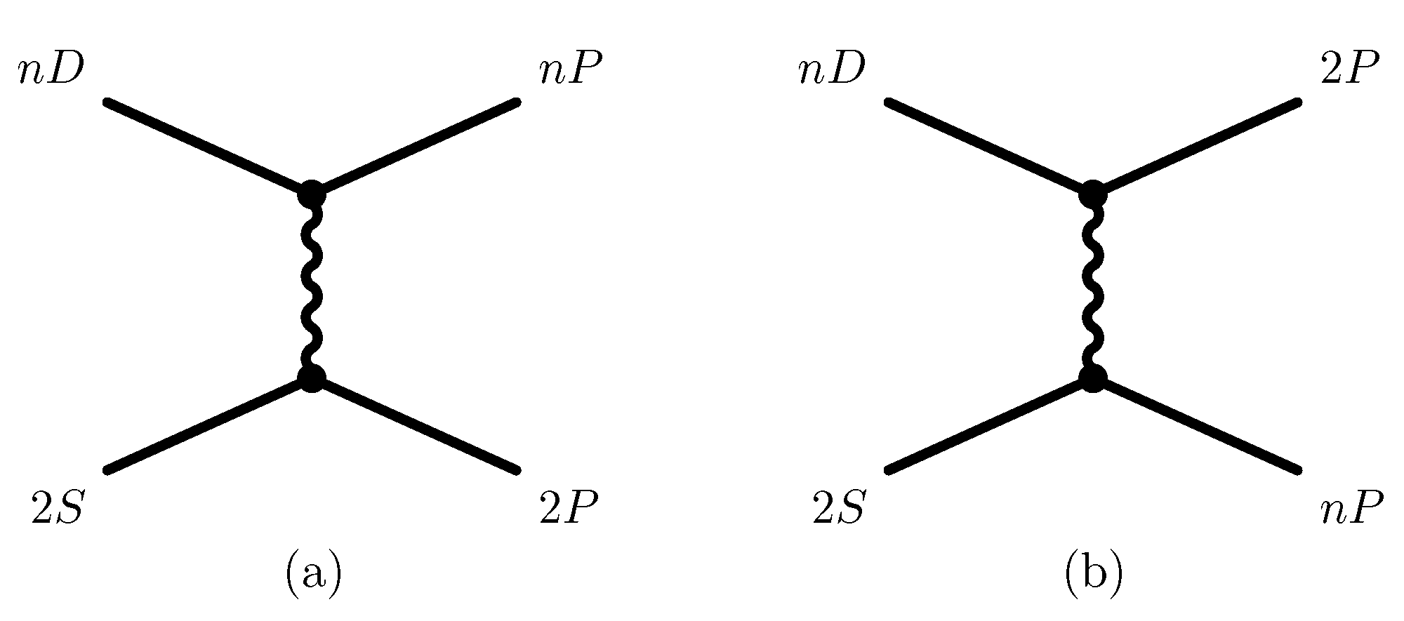
The leading-order contribution to the van-der Waals interaction is the dipole–dipole interaction, which reads

$$\begin{array}{c}\hfill H_{\mathrm{vdW}}\stackrel{l.o.}{=}{E}_h{a}_0\left[\frac{{\overrightarrow{𝓇}}_A·{\overrightarrow{𝓇}}_B}{R^3}-\frac{3\left(\overrightarrow{R}·{\overrightarrow{𝓇}}_A\right)\left(\overrightarrow{R}·{\overrightarrow{𝓇}}_B\right)}{R^5}\right]=\frac{e^2}{4\pi {ϵ}_0}\frac{x_A{x}_B+y_A{y}_B-2z_A{z}_B}{R^3},\end{array}$$

(9)

where we assume that the interatomic separation is aligned with the quantization axis, $\overrightarrow{R}=R{\widehat{\mathrm{e}}}_z$. The corresponding Feynman diagram for one-photon exchange (for the $(nD;2S)$ system, involving virtual P states) is depicted in Figure 1.

Figure 1. Feynman diagram for the one-photon exchange interaction within the quasi-degenerate basis of the $nD$ and $2S$ atoms. There are two combinations of final states possible within the manifolds of quasi-degenerate states investigated here, as evident from (a,b). Both processes are taken into account in our formalism. For $n=3$, the displayed diagrams constitute all diagrams relevant to the $1/R^6$ interaction; for $n=8$, there are two further diagrams where the $nP$ states is replaced by an $nF$ state. This is explained in further detail in Section 4.

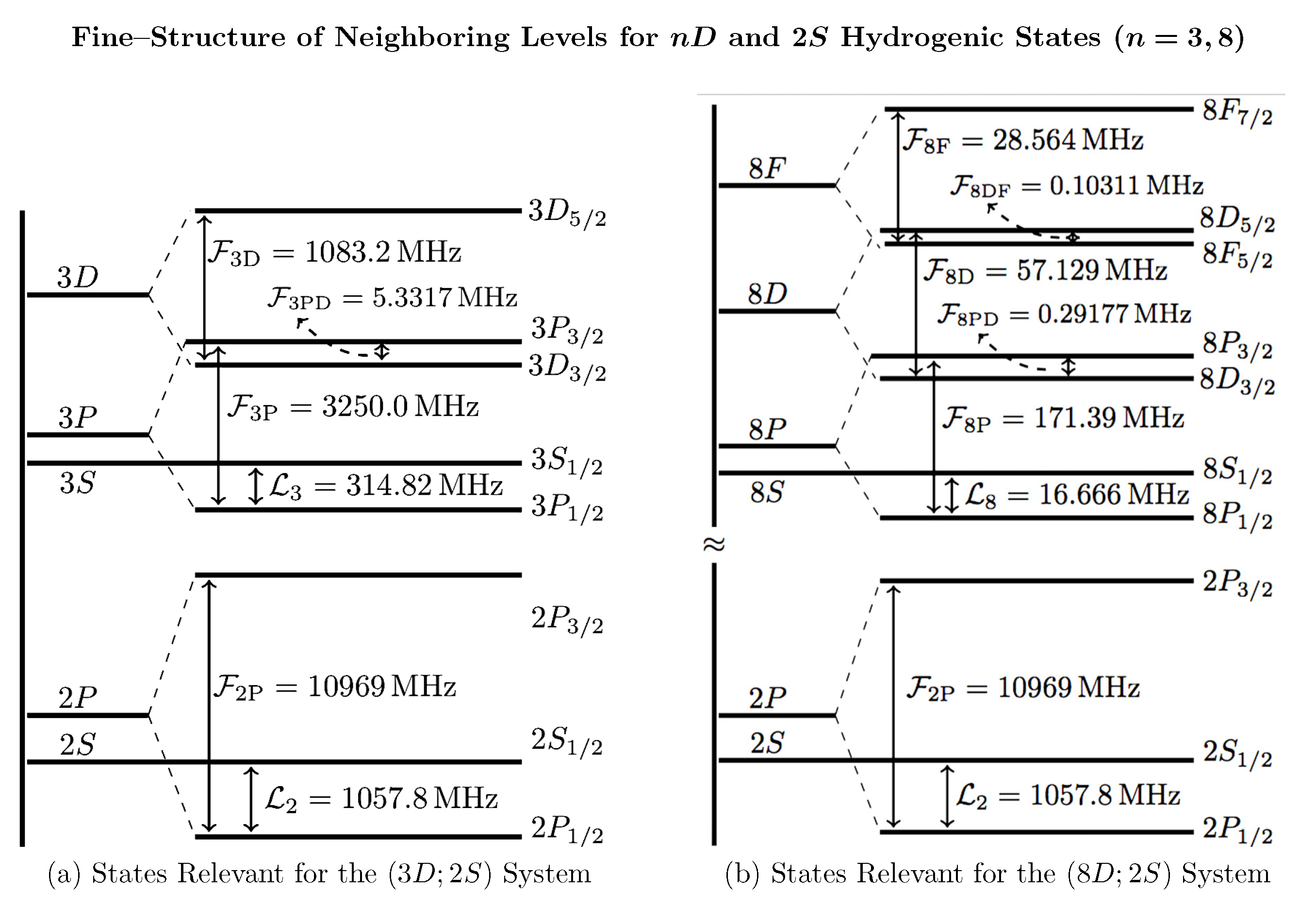
The role of the virtual $2P_{3/2}$ states is worthy of special attention. The $2S$ and $2P_{1/2}$ levels are displaced only by the classic Lamb shift, ${\mathcal{L}}_2$, while the $2P_{3/2}$ levels are displaced by the fine structure which is larger than the classic Lamb shift by an order of magnitude (see Figure 2). Because of this relatively large separation from the reference $2S$ level, we discard the $2P_{3/2}$ states. The theoretical accuracy of our results for the $C_6$ coefficients can thus be estimated to be on the order of roughly $10\%$. We stress that the main aim of our calculations is the determination of estimates of the $C_6$ coefficients for pressure shifts in atomic beams; the pressure shift is proportional to $|C_6{|}^{2/5}$ (see Ref. [6]). The resulting theoretical uncertainty of $4\%$ in the pressure shift is perfectly acceptable, both because the effect is small overall and because its determination depends on other parameters such as the volume density of atoms in the beam, which can typically be estimated only with much less precision [6]. Thus, here and in the following, whenever we discuss $n{P}_{3/2}$ levels, we do not mean $n=2$. The $3D_{3/2}$ and $3P_{3/2}$ levels are about $\sim 5$ MHz apart, and the separation between $8D_{3/2}$ and $8P_{3/2}$ levels is only about $\sim 0.29$ MHz. The spacing between $3P_{1/2}$ and $3P_{3/2}$ levels is about three orders of magnitude larger than the $3P_{3/2}$–$3D_{3/2}$ splitting (see Figure 2a). The same is true in the case of $8P_{1/2}$–$8P_{3/2}$ and $8P_{3/2}$–$8D_{3/2}$ spacings (see Figure 2b). The role of virtual $n{P}_{1/2}$ states is thus suppressed in comparison to virtual $n{P}_{3/2}$ states. The energetically quasi-degenerate $n{P}_{3/2}$–$n{D}_{3/2}$ transition plays a significant role in the long-range $nD$–$2S$ interaction.

Figure 2. Schematic diagram for energy levels showing the fine structure splittings for $n=2$ and $n=3$ levels (a) and $n=2$ and $n=8$ levels (b). The spacing between the energy levels are not scaled; some closely spaced splittings are exaggerated in comparison with the widely spaced ones for better visibility. In (b), instead of displaying all the energy levels for $n=3,4,\cdots ,7$, we introduced a break in the vertical axis. The $n{D}_{3/2}$–$n{D}_{5/2}$ and $n{P}_{1/2}$–$n{P}_{3/2}$ splittings are denoted as ${\mathcal{F}}_{n\mathrm{D}}$ and ${\mathcal{F}}_{n\mathrm{P}}$, respectively, while $n{P}_{3/2}$–$n{D}_{3/2}$ splittings are denoted as ${\mathcal{F}}_{n\mathrm{PD}}$.

When setting up the calculation, it is useful to define the following parameters:

$$\begin{array}{cc}\hfill \mathcal{H}& =\frac{g_N}{18}\frac{{\alpha }^4{m}_e^2{c}^2}{m_p}=59.21498\mathrm{MHz}=8.99967\times {10}^{-9}{E}_h,\hfill \end{array}$$

(10)

$$\begin{array}{cc}\hfill {\mathcal{L}}_2& =E\left(2P_{1/2}\right)-E\left(2S_{1/2}\right)=h1057.8447\mathrm{MHz}=1.60774\times {10}^{-7}{E}_h,\hfill \end{array}$$

(11)

$$\begin{array}{cc}\hfill {\mathcal{F}}_{3\mathrm{PD}}& =E\left(3P_{3/2}\right)-E\left(3D_{3/2}\right)=h5.33172\mathrm{MHz}=8.10331\times {10}^{-10}{E}_h,\hfill \end{array}$$

(12)

$$\begin{array}{cc}\hfill {\mathcal{F}}_{3\mathrm{D}}& =E\left(3D_{3/2}\right)-E\left(3D_{5/2}\right)=h1083.33970\mathrm{MHz}=1.64649\times {10}^{-7}{E}_h.\hfill \end{array}$$

(13)

The hyperfine parameter $\mathcal{H}$ is the hyperfine splitting between the $F=0$ hyperfine singlet and the $F=1$ hyperfine triplet of the $2P_{1/2}$ states; ${\mathcal{F}}_{3\mathrm{PD}}$ is fine-structure splitting between $3P_{3/2}$ and $3D_{3/2}$ levels whereas ${\mathcal{F}}_{3\mathrm{D}}$ is the fine-structure splitting between $3D_{3/2}$ and $3D_{5/2}$ levels of hydrogen atom [16]. Corresponding quantities for the $(8D;2S)$ system are defined in Figure 2b. Numerical values of fundamental physical constants are taken from Refs. [17,18]. One can calculate the ratios of energy level spacings given in Figure 2 and find that the Lamb shift ${\mathcal{L}}_n$ and the fine-structure splittings ${\mathcal{F}}_{n\mathrm{P}}$, ${\mathcal{F}}_{n\mathrm{D}}$, and ${\mathcal{F}}_{n\mathrm{PD}}$ approximately follow the $1/n^3$ scaling law, where n is the principal quantum number.

Due to the multitude of relevant levels in the $n=3$ and $n=8$ manifolds, it is alternatively possible to define the following parameters:

$$\Xi \left(n{\ell }_j\right)=\frac{E\left(n{\ell }_j\right)-E\left(n{P}_{1/2}\right)}{{\alpha }^5{m}_e{c}^2},$$

(14)

where $\Xi \left(n{\ell }_j\right)$ is a dimensionless parameter which expresses the energy displacement of the level with quantum numbers n, ℓ, and j from the energetically lowest level $n{P}_{1/2}$ within the manifold of given n in units of the Lamb shift scale ${\alpha }^5{m}_e{c}^2$. One may use the database [16] to obtain the following results:

$$\begin{array}{cc}\hfill \Xi \left(2P_{1/2}\right)=0,& \Xi \left(2S_{1/2}\right)=0.41373,\Xi \left(2P_{3/2}\right)=4.2901,\hfill \end{array}$$

(15)

$$\begin{array}{cc}\hfill \Xi \left(3P_{1/2}\right)=0,& \Xi \left(3S_{1/2}\right)=0.12315,\Xi \left(3D_{3/2}\right)=1.2691,\hfill \end{array}$$

(16)

$$\begin{array}{cc}\hfill \Xi \left(3P_{3/2}\right)=1.2711,& \Xi \left(3D_{5/2}\right)=1.6927,\hfill \end{array}$$

(17)

$$\begin{array}{cc}\hfill \Xi \left(8P_{1/2}\right)=0,& \Xi \left(8S_{1/2}\right)=0.006518,\hfill \end{array}$$

(18)

$$\begin{array}{cc}\hfill \Xi \left(8D_{3/2}\right)=0.066919,& \Xi \left(8P_{3/2}\right)=0.067033,\hfill \end{array}$$

(19)

$$\begin{array}{cc}\hfill \Xi \left(8F_{5/2}\right)=0.089222,& \Xi \left(8D_{5/2}\right)=0.089262,\Xi \left(8F_{7/2}\right)=0.100039.\hfill \end{array}$$

(20)

The smaller parameters for $n=8$ illustrate that the higher excited states are energetically closer than for $n=3$, which results in smaller propagator denominators and larger second-order long-range energy shifts.

To explain these ideas, a few remarks might be in order. An atom in a $2S$ state has four hyperfine states, namely, a hyperfine singlet for $F=0$ and a hyperfine triplet for $F=1$. The $nD$ states have $n{D}_{3/2}$ and $n{D}_{5/2}$ fine structures. For $n{D}_{3/2}$, the hyperfine quantum number F takes the values $F=1$ and $F=2$, while for $n{D}_{5/2}$ states, one either has $F=2$ or $F=3$. As a result, the $n{D}_{3/2}$ and $n{D}_{5/2}$ states further split into eight and twelve hyperfine states, respectively. For atomic states with $\ell =3$, one has hyperfine manifolds with $F=3$ and $F=4$. We here use the notation $|n,\ell ,j,F,F_z⟩$ to denote the basis states, where n is the principal quantum number, ℓ is the orbital quantum number, and j is the total (orbital + spin) electronic angular momentum quantum number. Furthermore, we denote by F the overall total (orbital + electron spin + nuclear spin) angular momentum quantum number. The projection of the overall total angular momentum quantum number onto the quantization axis (z axis, aligned with the interatomic separation) of an individual atomic electron is denoted as $F_z$ (or, as $F_{z,i}$ with $i=A,B$ if the specification of the atom is not clear from the context). For the two atoms, we anticipate that the total overall angular momentum projection is ${\mathcal{F}}_z=F_{z,A}+F_{z,B}$ as the sum of the projections for the electrons in atoms A and B. The quantum number ${\mathcal{F}}_z$ is a conserved quantity under the long-range interaction and allows us to separate the Hamiltonian matrices into mutually noninteracting submanifolds.

The unperturbed states in our problem are thus the states

$$|\varphi ⟩=|{(n_A,{\ell }_A,j_A,F_A,F_{z,A})}_A{(n_B,{\ell }_B,j_B,F_B,F_{z,B})}_B⟩,$$

(21)

with both hydrogen atoms in well-defined hyperfine states. The hyperfine states are constructed from the states $|n,\ell ,j⟩$ via the addition of the nuclear angular momentum. Conversely, one establishes, with reference to Equation (5), the diagonality of the Lamb shift Hamiltonian in the hyperfine basis:

$$⟨n_i,{\ell }_i,j_i,F_i,F_{z,i}\left|H_{\mathrm{LS},i}\right|n_i^{\prime },{\ell }_i^{\prime },j_i^{\prime },F_i^{\prime },F_{z,i}^{\prime }⟩=⟨n_i,{\ell }_i,j_i\left|H_{\mathrm{LS},i}\right|n_i^{\prime },{\ell }_i^{\prime },j_i^{\prime }⟩{\delta }_{F_i{F}_i^{\prime }}{\delta }_{F_{z,i}{F}_{z,i}^{\prime }}.$$

(22)

In this context, it is useful to remember that hyperfine effects are excluded from the energy levels of states $|n,\ell ,j⟩$ given in the database [16]. This observation applies to the definition of the $\Xi$ parameters in Equation (14).

Let us now briefly discuss the evaluation of the diagonal elements of the hyperfine Hamiltonian, noting that we can temporarily drop the index $i=A,B$ indicating the atom, since we are dealing with two identical hydrogen atoms. The expectation value of $H_{\mathrm{HFS}}$ measures the diagonal entries of the hyperfine splitting Hamiltonian, and it reads [19]

$$\begin{array}{cc}\hfill E_{\mathrm{HFS}}(n,\ell ,j,F)=& \left.⟨n,\ell ,j,I,F,F_z\right|H_{\mathrm{HFS}}\left|n,\ell ,I,F,F_z\right.⟩\hfill \\ \hfill =& \frac{\alpha g_N}{2}\frac{m_e^2}{m_p}{\xi }_e(\ell ,j)\left[F(F+1))-I(I+1)-j(j+1)\right],\hfill \end{array}$$

(23)

where $m_p$ is the proton mass. The quantity ${\xi }_e(\ell ,j)$ depends only on the electronic part. In the nonrelativistic limit, one obtains the following results [19]:

$$\begin{array}{c}\hfill {\xi }_e(0,\frac{1}{2})=\frac{4{\alpha }^3{m}_e{c}^2}{3n^3},{\xi }_e(1,\frac{1}{2})=\frac{4{\alpha }^3{m}_e{c}^2}{9n^3},{\xi }_e(1,\frac{3}{2})=\frac{4{\alpha }^3{m}_e{c}^2}{45n^3},\end{array}$$

(24)

$$\begin{array}{c}\hfill {\xi }_e(2,\frac{3}{2})=\frac{4{\alpha }^3{m}_e{c}^2}{75n^3},{\xi }_e(2,\frac{5}{2})=\frac{4{\alpha }^3{m}_e{c}^2}{175n^3},{\xi }_e(3,\frac{5}{2})=\frac{4{\alpha }^3{m}_e{c}^2}{245n^3},\end{array}$$

(25)

$$\begin{array}{c}\hfill {\xi }_e(3,\frac{7}{2})=\frac{4{\alpha }^3{m}_e{c}^2}{441n^3}.\end{array}$$

(26)

The proton spin is $I=1/2$. For all hydrogenic states of interest, Equations (23) and (24) define the hyperfine splitting uniquely. An example is the hyperfine energy shift of $2S$ states:

$$E_{\mathrm{HFS}}(n=2,\ell =0,j=\frac{1}{2},F)=\frac{g_N}{12}\frac{{\alpha }^4{m}_e^2{c}^2}{m_p}\left[F(F+1)-\frac{3}{2}\right].$$

(27)

For $8F_{5/2}$ and $8F_{7/2}$ states, one obtains the results

$$\begin{array}{cc}\hfill E_{\mathrm{HFS}}(n=8,\ell =3,j=\frac{5}{2},F)=& \frac{g_N{\alpha }^4{m}_e^2{c}^2}{62720m_p}\left[F(F+1)-\frac{19}{2}\right],\hfill \end{array}$$

(28)

$$\begin{array}{cc}\hfill E_{\mathrm{HFS}}(n=8,\ell =3,j=\frac{7}{2},F)=& \frac{g_N{\alpha }^4{m}_e^2{c}^2}{112896m_p}\left[F(F+1)-\frac{33}{2}\right].\hfill \end{array}$$

(29)

It is well known that the hyperfine Hamiltonian has off-diagonal elements in the fine-structure resolved basis. The relevant off-diagonal elements of the hyperfine Hamiltonian for the $(nD;2S)$ reference states under investigation are given by

$$\begin{array}{cc}\hfill & \left.⟨n=3,\ell =2,j=\frac{5}{2},F=2,F_z\right|H_{\mathrm{H}FS}\left|n=3,\ell =2,j^{\prime }=\frac{3}{2},F=2,F_z\right.⟩\hfill \\ \hfill & =-\frac{g_N{\alpha }^4{m}_e^2{c}^2}{1350\sqrt{6}{m}_p},\hfill \end{array}$$

(30)

$$\begin{array}{cc}\hfill & \left.⟨n=8,\ell =2,j=\frac{5}{2},F=2,F_z\right|H_{\mathrm{H}FS}\left|n=8,\ell =2,j^{\prime }=\frac{3}{2},F=2,F_z\right.⟩\hfill \\ \hfill & =-\frac{g_N{\alpha }^4{m}_e^2{c}^2}{25600\sqrt{6}{m}_p}.\hfill \end{array}$$

(31)

The nontrivial off-diagonal matrix elements are incurred for $n{D}_{3/2}$ and $n{D}_{5/2}$ states with the same overall total angular momentum quantum number $F=2$ and the same $F_z$. It is evident from the ratio of Equation (30) to Equation (31), i.e., $8^3:3^3$, that the off-diagonal hyperfine splitting follows the $1/n^3$ scaling.

A rediagonalization of the hyperfine Hamiltonian in the basis of states

$$\begin{array}{c}\hfill |a⟩=\left|n{D}_{3/2}^{F=2}\left(F_z\right)\right.⟩=\left|n,2,\frac{3}{2},2,F_z\right.⟩,|b⟩=\left|n{D}_{5/2}^{F=2}\left(F_z\right)\right.⟩=\left|n,2,\frac{5}{2},2,F_z\right.⟩,\end{array}$$

(32)

leads to the following second-order energy shifts:

$$\begin{array}{c}\hfill \Delta E^{\left(2\right)}(3D;F=2)=\frac{1}{33750}\frac{{\mathcal{H}}^2}{\frac{4}{75}\mathcal{H}+{\mathcal{F}}_{3D}}={\Delta }_3{E}_h,{\Delta }_3=1.4618\times {10}^{-14},\end{array}$$

(33)

$$\begin{array}{c}\hfill \Delta E^{\left(2\right)}(8D;F=2)=\frac{27}{327680000}\frac{{\mathcal{H}}^2}{\frac{9}{3200}\mathcal{H}+{\mathcal{F}}_{8D}}={\Delta }_8{E}_h,{\Delta }_8=7.7087\times {10}^{-16}.\end{array}$$

(34)

Taking the ratio of the $\Delta$s from Equations (33) and (34), we have ${\Delta }_3:{\Delta }_8\approx 8^3:3^3$, consistent with the fact that ${\Delta }_n\sim 1/n^3$.

3. Second–Order van-der-Waals Shifts in the $(3D;2S)$ System

The calculation proceeds as follows. The reference states are $(3D;2S)$ states, with one atom in the metastable $2S$ state and the other in the excited $3D$ state. One includes virtual $(3P;2P)$ states that could be reached via electric dipole transitions and have nonvanishing transition matrix elements with the Hamiltonian (9). Specifically, for the reasons outlined above, one investigates the manifolds composed of the product states of $2S_{1/2}(F=0,1)$, $2P_{1/2}(F=0,1)$, $3P_{1/2}(F=0,1)$, $3P_{3/2}(F=1,2)$, $3D_{3/2}(F=1,2)$, and $3D_{5/2}(F=2,3)$. Of the product states, only the $(3D;2S)$ states could be interpreted as reference states. The total number of states is $4+4+4+8+8+12=40$. These states could in principle form ${40}^2=1600$ product states in hyperfine resolution, which all should be analyzed. However, we can select from the product states only those that are energetically quasi-degenerate with respect to the reference states. The physically relevant basis states have $n_A+n_B=5$ for the $(3D;2S)$ interaction and ${\ell }_A+{\ell }_B=2$. Namely, for ${\ell }_A=0$ and ${\ell }_B=2$, one has a reference state, while for ${\ell }_A={\ell }_B=1$, one has a virtual state composed of two P states. Here, $n_i$ and ${\ell }_i$ are the principal and the orbital angular quantum numbers, respectively, of the ith atom $(i=A,B)$. The van-der-Waals Hamiltonian (9) is diagonal in the quantum number

$${\mathcal{F}}_z=F_{z,A}+F_{z,B},$$

(35)

which is the sum of the two projections of atoms A and B. One can easily find that the nine physically relevant hyperfine manifolds are those with ${\mathcal{F}}_z=0,\pm 1,\pm 2,\pm 3,\pm 4$. The two reference states in the ${\mathcal{F}}_z=4$ hyperfine manifold are (see also Table 1),

$$\begin{array}{c}\hfill |{\psi }_1⟩=|2,0,\frac{1}{2}{,1,1⟩}_A|n,2,\frac{5}{2}{,3,3⟩}_B,|{\psi }_2⟩=|n,2,\frac{5}{2}{,3,3⟩}_A{|2,0,\frac{1}{2},1,1⟩}_B.\end{array}$$

(36)

Table 1. Multiplicities are given for reference $(n{D}_{j=3/2,j=5/2};2S)$ states, in the submanifolds with different ${\mathcal{F}}_z=0,\pm 1,\pm 2,\pm 3,\pm 4$. For reference, we point out that the highest ${\mathcal{F}}_z$ value (${\mathcal{F}}_z=4$) is reached for reference states composed of the $F=3$ hyperfine submanifold of the $D_{5/2}$ states with maximum projection on the quantization axis, and the $F=1$ hyperfine submanifold of the $S_{1/2}$ states, also with maximum projection on the quantization axis. Entries marked with a long hyphen (–) indicate unphysical combinations.

$({\mathit{j}}_{\mathit{A}},{\mathit{F}}_{\mathit{A}})$	${\mathcal{F}}_{\mathit{z}}=0$	${\mathcal{F}}_{\mathit{z}}=\pm 1$	${\mathcal{F}}_{\mathit{z}}=\pm 2$	${\mathcal{F}}_{\mathit{z}}=\pm 3$	${\mathcal{F}}_{\mathit{z}}=\pm 4$	Total
$(\frac{5}{2},3)$	8	8	8	6	2	56
$(\frac{5}{2},2)$	8	8	6	2	–	40
$(\frac{3}{2},2)$	8	8	6	2	–	40
$(\frac{3}{2},1)$	8	6	2	–	–	24
Total	32	30	22	10	2	160

The ${\mathcal{F}}_z=4$ manifold does not involve any quasi-degenerate $(P;P)$ states that could be reached via dipole transitions (remember that we exclude $2P_{3/2}$ states); hence, the second-order energy shift vanishes (see also Table 2). The manifolds with ${\mathcal{F}}_z=\pm 3$ have 12 quasi-degenerate states, while for ${\mathcal{F}}_z=\pm 2$, one has 32 quasi-degenerate states. For ${\mathcal{F}}_z=\pm 1$, one encounters 52 states, while for ${\mathcal{F}}_z=0$, one has 60 states. For an example of a matrix obtained for a given value of ${\mathcal{F}}_z$ in a related calculation for a different atomic-state configuration, we refer to Section 3.4 of Ref. [5]. Our calculation reported here proceeds analogously, but with even higher-dimensional matrices for each ${\mathcal{F}}_z$ as compared to Ref. [5].

Table 2. Second-order van-der-Waals shifts of the $1/R^6$-type are given for $3D_j$ hydrogen atoms interacting with $2S$-state hydrogen via virtual P states. Entries marked with a long hyphen (–) indicate unphysical combinations of F and ${\mathcal{F}}_z$ values, within our basis of states. We denote the scaled interatomic distance by $\rho =R/a_0$ and give all energy shifts in atomic units, i.e., in units of the Hartree energy $E_h={\alpha }^2{m}_e{c}^2$. The symbol ${\Delta }_3$ denotes the fine-structure-hyperfine-structure mixing term, which is given in Equation (33). Recall that ${\mathcal{F}}_z=F_{z,A}+F_{z,B}$; however, the $F_A$ quantum number in the table is that of the $3D_j$ state, which constitutes the reference state.

$({\mathit{j}}_{\mathit{A}},{\mathit{F}}_{\mathit{A}})$	${\mathcal{F}}_{\mathit{z}}=0$	${\mathcal{F}}_{\mathit{z}}=\pm 1$	${\mathcal{F}}_{\mathit{z}}=\pm 2$	${\mathcal{F}}_{\mathit{z}}=\pm 3$	${\mathcal{F}}_{\mathit{z}}=\pm 4$
$(\frac{5}{2},3)$	${\displaystyle \frac{1.0743\times {10}^9}{{\rho }^6}}$	${\displaystyle \frac{9.9925\times {10}^8}{{\rho }^6}}$	${\displaystyle \frac{7.7411\times {10}^8}{{\rho }^6}}$	${\displaystyle \frac{4.2149\times {10}^8}{{\rho }^6}}$	0
$(\frac{5}{2},2)$	$1.0595\times {10}^9/{\rho }^6+{\Delta }_3$	$9.0978\times {10}^8/{\rho }^6+{\Delta }_3$	$5.4505\times {10}^8/{\rho }^6+{\Delta }_3$	$9.8638\times {10}^7/{\rho }^6+{\Delta }_3$	–
$(\frac{3}{2},2)$	$9.5443\times {10}^8/{\rho }^6-{\Delta }_3$	$8.7210\times {10}^8/{\rho }^6-{\Delta }_3$	$6.8471\times {10}^8/{\rho }^6-{\Delta }_3$	$4.3899\times {10}^8/{\rho }^6-{\Delta }_3$	–
$(\frac{3}{2},1)$	${\displaystyle \frac{8.9169\times {10}^8}{{\rho }^6}}$	${\displaystyle \frac{7.8772\times {10}^8}{{\rho }^6}}$	${\displaystyle \frac{5.4296\times {10}^8}{{\rho }^6}}$	–	–

For clarity, we thus present one particular case, namely, the ${\mathcal{F}}_z=4$ submanifold for the $(8D;2S)$ system, in Section 4. Note also that, as explained in the discussion following Equation (9), the final results for the $C_6$ coefficients have a theoretical uncertainty of roughly 10%. We still indicate the results in Table 2 to five significant figures, in order to facilitate an accurate independent recalculation of the coefficients within the indicated, specified basis set of states. The quoted accuracy is thus nominal and does not imply that all indicated figures are physically significant.

One then selects from every ${\mathcal{F}}_z$ manifold the reference $(3D;2S)$ states with the defined ${\mathcal{F}}_z$ eigenvalue and then calculates the second-order shifts due to all $(3P;2P)$ hyperfine sublevels coupled to the reference level via the van-der-Waals Hamiltonian. One verifies that the first-order shifts vanish when the average is taken in a specific ${\mathcal{F}}_z$ manifold, which makes the first-order shifts physically irrelevant [6]. One may average the second-order shifts in various ways. For a given ${\mathcal{F}}_z$ value, when averaging over the possible j and F values of the excited D state, one obtains the the following results after the extensive use of computer algebra [20],

$$\begin{array}{cc}\hfill {⟨E(3D,{\mathcal{F}}_z=0)⟩}_{j,F}=& \frac{9.9498\times {10}^8{E}_h}{{\rho }^6},\hfill \end{array}$$

(37)

$$\begin{array}{cc}\hfill {⟨E(3D,{\mathcal{F}}_z=\pm 1)⟩}_{j,F}=& \frac{8.9918\times {10}^8{E}_h}{{\rho }^6},\hfill \end{array}$$

(38)

$$\begin{array}{cc}\hfill {⟨E(3D,{\mathcal{F}}_z=\pm 2)⟩}_{j,F}=& \frac{6.6624\times {10}^8{E}_h}{{\rho }^6},\hfill \end{array}$$

(39)

$$\begin{array}{cc}\hfill {⟨E(3D,{\mathcal{F}}_z=\pm 3)⟩}_{j,F}=& \frac{3.6042\times {10}^8{E}_h}{{\rho }^6},\hfill \end{array}$$

(40)

$$\begin{array}{cc}\hfill {⟨E(3D,{\mathcal{F}}_z=\pm 4)⟩}_{j,F}=& 0.\hfill \end{array}$$

(41)

When averaging over ${\mathcal{F}}_z$ for given j and F, one has

$$\begin{array}{cc}\hfill {⟨E(3D_{5/2},F=3)⟩}_{{\mathcal{F}}_z}=& \frac{7.5046\times {10}^8{E}_h}{{\rho }^6},\hfill \end{array}$$

(42)

$$\begin{array}{cc}\hfill {⟨E(3D_{5/2},F=2)⟩}_{{\mathcal{F}}_z}=& \left({\Delta }_3+\frac{7.4919\times {10}^8}{{\rho }^6}\right)E_h,\hfill \end{array}$$

(43)

$$\begin{array}{cc}\hfill {⟨E(3D_{3/2},F=2)⟩}_{{\mathcal{F}}_z}=& \left(-{\Delta }_3+\frac{7.8904\times {10}^8}{{\rho }^6}\right)E_h,\hfill \end{array}$$

(44)

$$\begin{array}{cc}\hfill {⟨E(3D_{3/2},F=1)⟩}_{{\mathcal{F}}_z}=& \frac{7.8158\times {10}^9{E}_h}{{\rho }^6}.\hfill \end{array}$$

(45)

The fine-structure averages, keeping j fixed but averaging over F and ${\mathcal{F}}_z$, are given as

$$\begin{array}{cc}\hfill {⟨E\left(3D_{5/2}\right)⟩}_{F,{\mathcal{F}}_z}=& \left(\frac{5}{12}{\Delta }_3+\frac{7.4993\times {10}^8}{{\rho }^6}\right)E_h,\hfill \end{array}$$

(46)

$$\begin{array}{cc}\hfill {⟨E\left(3D_{3/2}\right)⟩}_{F,{\mathcal{F}}_z}=& \left(-\frac{5}{8}{\Delta }_3+\frac{7.8624\times {10}^8}{{\rho }^6}\right)E_h.\hfill \end{array}$$

(47)

Recall that ${\Delta }_3$ is given in Equation (33).

4. Second–Order van-der-Waals Shifts in the $(8D;2S)$ System

One proceeds similar to the $(3D;2S)$ case. With the reference $(8D;2S)$ states, one includes virtual $(8P;2P)$ and virtual $(8F;2P)$ states that could be reached via electric dipole transitions and have nonvanishing transition matrix elements with the Hamiltonian (9). Specifically, one investigates the manifolds composed of the product states of $2S_{1/2}(F=0,1)$, $2P_{1/2}(F=0,1)$, $8P_{1/2}(F=0,1)$, $8P_{3/2}(F=1,2)$, $8D_{3/2}(F=1,2)$, and $8D_{5/2}(F=2,3)$, as well as $8F_{5/2}(F=2,3)$ and $8F_{7/2}(F=3,4)$. Only the hyperfine manifolds of the $(8D;2S)$ states act as reference states. The total number of states is $4+4+4+8+8+12+12+16=68$ states. Of the ${68}^2=4624$ product states, one can select only those which are energetically quasi-degenerate with respect to the reference states. The relevant basis states have $n_A+n_B=10$ for the $(8D;2S)$ interaction, and ${\ell }_A+{\ell }_B=2$ and/or ${\ell }_A+{\ell }_B=4$ (virtual $(F;P)$ states). For ${\ell }_A=0$ and ${\ell }_B=2$, one has a reference state, while for ${\ell }_A={\ell }_B=1$, ${\ell }_A=1$, and ${\ell }_B=3$, one has virtual states. Here, again, $n_i$ and ${\ell }_i$ are the principal and the orbital angular quantum numbers of the ith atom $(i=A,B)$. Since the van-der-Waals Hamiltonian (9) is diagonal in the quantum number ${\mathcal{F}}_z=F_{z,A}+F_{z,B}$, one can diagonalize the interaction in the submanifolds with ${\mathcal{F}}_z=0,\pm 1,\pm 2,\pm 3,\pm 4,\pm 5$ separately. For our purposes, the submanifold with ${\mathcal{F}}_z=\pm 5$ is physically irrelevant because it does not contain $(8D;2S)$ reference states.

For the $(8D;2S)$ system, one needs to consider a complicated array of virtual P and F states. The manifold with ${\mathcal{F}}_z=4$ (which contains 12 quasi-degenerate states) provides us with an opportunity to illustrate the calculation by way of and example. To this end, we supplement the definition given in Equations (10)–(13) as follows:

$$\mathcal{V}\equiv 3\frac{e^2}{4\pi {ϵ}_0}\frac{a_0^2}{R^3}=\frac{3E_h}{{\rho }^3},$$

(48)

where $\mathcal{V}$ measures the characteristic scale of a first-order element of the nonretarded van-der-Waals interaction, and the interatomic distance, expressed in atomic units, is denoted as $\rho =R/a_0$. The first six states, given in the notation introduced in Equation (21), in the manifold with ${\mathcal{F}}_z=4$. are as follows,

$$\begin{array}{cccc}\hfill |{\varphi }_1⟩=& |{(2,0,\frac{1}{2},1,1)}_A{(8,2,\frac{5}{2},3,3)}_B⟩,\hfill & \hfill |{\varphi }_2⟩& =|{(2,1,\frac{1}{2},0,0)}_A{(8,3,\frac{7}{2},4,4)}_B⟩,\hfill \end{array}$$

(49)

$$\begin{array}{cccc}\hfill |{\varphi }_3⟩=& |{(2,1,\frac{1}{2},1,0)}_A{(8,3,\frac{7}{2},4,4)}_B⟩,\hfill & \hfill |{\varphi }_4⟩& =|{(2,1,\frac{1}{2},1,1)}_A{(8,3,\frac{5}{2},3,3)}_B⟩,\hfill \end{array}$$

(50)

$$\begin{array}{cccc}\hfill |{\varphi }_5⟩=& |{(2,1,\frac{1}{2},1,1)}_A{(8,3,\frac{7}{2},3,3)}_B⟩,\hfill & \hfill |{\varphi }_6⟩& =|{(2,1,\frac{1}{2},1,1)}_A{(8,3,\frac{7}{2},4,3)}_B⟩.\hfill \end{array}$$

(51)

They are complemented by six further states with ${\mathcal{F}}_z=4$,

$$\begin{array}{cccc}\hfill |{\varphi }_7⟩=& |{(8,2,\frac{5}{2},3,3)}_A{(2,0,\frac{1}{2},1,1)}_B⟩,\hfill & \hfill |{\varphi }_8⟩& =|{(8,3,\frac{5}{2},3,3)}_A{(2,1,\frac{1}{2},1,1)}_B⟩,\hfill \end{array}$$

(52)

$$\begin{array}{cccc}\hfill |{\varphi }_9⟩=& |{(8,3,\frac{7}{2},3,3)}_A{(2,1,\frac{1}{2},1,1)}_B⟩,\hfill & \hfill |{\varphi }_{10}⟩& =|{(8,3,\frac{7}{2},4,3)}_A{(2,1,\frac{1}{2},1,1)}_B⟩,\hfill \end{array}$$

(53)

$$\begin{array}{cccc}\hfill |{\varphi }_{11}⟩=& |{(8,3,\frac{7}{2},4,4)}_A{(2,1,\frac{1}{2},0,0)}_B⟩,\hfill & \hfill |{\varphi }_{12}⟩& =|{(8,3,\frac{7}{2},4,4)}_A{(2,1,\frac{1}{2},1,0)}_B⟩.\hfill \end{array}$$

(54)

In the basis of states $|{\varphi }_{i=1,\cdots ,6}⟩$, the matrix of the total Hamiltonian defined in Equation (1) is

$$\begin{array}{c}\hfill H^{\prime }=\left(\begin{array}{cccccc}{E}_{0,\frac{1}{2}}^{2,\frac{5}{2}}+\frac{6729\mathcal{H}}{8960}& -12\sqrt{\frac{55}{7}}\mathcal{V}& 12\sqrt{\frac{55}{7}}\mathcal{V}& -\frac{8\sqrt{165}}{7}\mathcal{V}& -\frac{12\sqrt{55}}{7}\mathcal{V}& 12\sqrt{\frac{55}{7}}\mathcal{V}\\ -12\sqrt{\frac{55}{7}}\mathcal{V}& E_{1,\frac{1}{2}}^{3,\frac{7}{2}}-\frac{1343}{1792}\mathcal{H}& 0& 0& 0& 0\\ 12\sqrt{\frac{55}{7}}\mathcal{V}& 0& E_{1,\frac{1}{2}}^{3,\frac{7}{2}}+\frac{449}{1792}\mathcal{H}& 0& 0& 0\\ -\frac{8\sqrt{165}}{7}\mathcal{V}& 0& 0& E_{1,\frac{1}{2}}^{3,\frac{5}{2}}+\frac{3145}{12544}\mathcal{H}& -\frac{3\sqrt{3}\mathcal{H}}{50176}& 0\\ -\frac{12\sqrt{55}}{7}\mathcal{V}& 0& 0& -\frac{3\sqrt{3}}{50176}\mathcal{H}& E_{1,\frac{1}{2}}^{3,\frac{7}{2}}+\frac{3127}{12544}\mathcal{H}& 0\\ 12\sqrt{\frac{55}{7}}\mathcal{V}& 0& 0& 0& 0& E_{1,\frac{1}{2}}^{3,\frac{7}{2}}+\frac{449}{1792}\mathcal{H}\end{array}\right).\end{array}$$

(55)

Here,

$$E_{\ell ,j}^{{\ell }^{\prime },j^{\prime }}=E_{n=2,\ell ,j}+E_{n=8,{\ell }^{\prime },j^{\prime }}$$

(56)

is a concise notation for the unperturbed energy levels without hyperfine effects. The energy level $E_{n,\ell ,j}=E\left(n{\ell }_j\right)$ enters the definition of the $\Xi$ parameter according to Equation (14). Now, in the basis of states $|{\varphi }_{i=7,\cdots ,12}⟩$, the Hamiltonian matrix of the total Hamiltonian defined in Equation (1) can be calculated as

$$\begin{array}{c}\hfill H^{″}=\left(\begin{array}{cccccc}{E}_{0,\frac{1}{2}}^{2,\frac{5}{2}}+\frac{6729}{8960}\mathcal{H}& -\frac{8\sqrt{165}\mathcal{V}}{7}& -\frac{12\sqrt{55}\mathcal{V}}{7}& 12\sqrt{\frac{55}{7}}\mathcal{V}& -12\sqrt{\frac{55}{7}}\mathcal{V}& 12\sqrt{\frac{55}{7}}\mathcal{V}\\ -\frac{8\sqrt{165}}{7}\mathcal{V}& E_{1,\frac{1}{2}}^{3,\frac{5}{2}}+\frac{3145}{12544}\mathcal{H}& -\frac{3\sqrt{3}}{50176}\mathcal{H}& 0& 0& 0\\ -\frac{12\sqrt{55}}{7}\mathcal{V}& -\frac{3\sqrt{3}}{50176}\mathcal{H}& E_{1,\frac{1}{2}}^{3,\frac{7}{2}}+\frac{3127}{12544}\mathcal{H}& 0& 0& 0\\ 12\sqrt{\frac{55}{7}}\mathcal{V}& 0& 0& E_{1,\frac{1}{2}}^{3,\frac{7}{2}}+\frac{449}{1792}\mathcal{H}& 0& 0\\ -12\sqrt{\frac{55}{7}}\mathcal{V}& 0& 0& 0& E_{1,\frac{1}{2}}^{3,\frac{7}{2}}-\frac{1343}{1792}\mathcal{H}& 0\\ 12\sqrt{\frac{55}{7}}\mathcal{V}& 0& 0& 0& 0& E_{1,\frac{1}{2}}^{3,\frac{7}{2}}+\frac{449}{1792}\mathcal{H}\end{array}\right).\end{array}$$

(57)

The Hamiltonian for ${\mathcal{F}}_z=4$ in in the basis of the twelve states listed in Equations (49)—(54) is

$$H_{{\mathcal{F}}_z=4}=\left(\begin{array}{cc}{H}^{\prime }& 0_{6\times 6}\\ 0_{6\times 6}& H^{″}\end{array}\right),$$

(58)

where $0_{6\times 6}$ is a 6-by-6 matrix with zero entries. For the manifolds with ${\mathcal{F}}_z=\pm 3$, we already have 34 quasi-degenerate states and the presentation of the Hamiltonian matrix is not practical. For ${\mathcal{F}}_z=\pm 2$, one already has 62 quasi-degenerate states. For ${\mathcal{F}}_z=\pm 1$, one encounters 84 states, while for ${\mathcal{F}}_z=0$, one has 92 states in the quasi-degenerate, hyperfine-resolved basis. One then proceeds as in the $(3D;2S)$ case, selects the reference states, and calculates the second-order shifts in the quasi-degenerate bases. When averaging over j and F for a given ${\mathcal{F}}_z$, one obtains

$$\begin{array}{cc}\hfill {⟨E(8D,{\mathcal{F}}_z=0)⟩}_{j,F}=& \frac{3.4778\times {10}^{11}{E}_h}{{\rho }^6},\hfill \end{array}$$

(59)

$$\begin{array}{cc}\hfill {⟨E(8D,{\mathcal{F}}_z=\pm 1)⟩}_{j,F}=& \frac{3.2626\times {10}^{11}{E}_h}{{\rho }^6},\hfill \end{array}$$

(60)

$$\begin{array}{cc}\hfill {⟨E(8D,{\mathcal{F}}_z=\pm 2)⟩}_{j,F}=& \frac{2.8373\times {10}^{11}{E}_h}{{\rho }^6},\hfill \end{array}$$

(61)

$$\begin{array}{cc}\hfill {⟨E(8D,{\mathcal{F}}_z=\pm 3)⟩}_{j,F}=& \frac{2.4342\times {10}^{11}{E}_h}{{\rho }^6},\hfill \end{array}$$

(62)

$$\begin{array}{cc}\hfill {⟨E(8D,{\mathcal{F}}_z=\pm 4)⟩}_{j,F}=& \frac{2.0722\times {10}^{11}{E}_h}{{\rho }^6}.\hfill \end{array}$$

(63)

Of particular interest is the global hyperfine average of the second-order van-der-Waals shifts over all possible $F_z$ values for given values of j and F (see also Table 3):

$$\begin{array}{cc}\hfill {⟨E(8D_{5/2},F=3)⟩}_{F_z}=& \frac{3.0674\times {10}^{11}{E}_h}{{\rho }^6},\hfill \end{array}$$

(64)

$$\begin{array}{cc}\hfill {⟨E(8D_{5/2},F=2)⟩}_{F_z}=& \left({\Delta }_8+\frac{3.0673\times {10}^{11}}{{\rho }^6}\right)E_h,\hfill \end{array}$$

(65)

$$\begin{array}{cc}\hfill {⟨E(8D_{3/2},F=2)⟩}_{F_z}=& \left(-{\Delta }_8+\frac{3.0378\times {10}^{11}}{{\rho }^6}\right)E_h,\hfill \end{array}$$

(66)

$$\begin{array}{cc}\hfill {⟨E(8D_{3/2},F=1)⟩}_{F_z}=& \frac{3.0377\times {10}^{11}{E}_h}{{\rho }^6}.\hfill \end{array}$$

(67)

Table 3. Second-order van-der-Waals shifts of the $1/R^6$-type are given for $8D_j$ hydrogen atoms interacting with $2S$-state hydrogen atoms in the presence of virtual P states. Just as in Table 2, entries marked with a long hyphen (–) indicate unphysical combinations of F and ${\mathcal{F}}_z$ values. The interatomic distance in atomic units is denoted as $\rho =R/a_0$. All energy shifts are given in Hartrees. The quantity ${\Delta }_8$ constitutes the fine-structure-hyperfine-structure mixing term, which is given in Equation (34). Recall that $F_z=F_{z,A}+F_{z,B}$; however, the $F_A$-number in the table is for the reference $8D_j$ state.

(${\mathit{j}}_{\mathit{A}},{\mathit{F}}_{\mathit{A}}$)	${\mathcal{F}}_{\mathit{z}}$ = 0	${\mathcal{F}}_{\mathit{z}}=\pm 1$	${\mathcal{F}}_{\mathit{z}}=\pm 2$	${\mathcal{F}}_{\mathit{z}}=\pm 3$	${\mathcal{F}}_{\mathit{z}}=\pm 4$
$(\frac{5}{2},3)$	${\displaystyle \frac{3.6868\times {10}^{11}}{{\rho }^6}}$	${\displaystyle \frac{3.5107\times {10}^{11}}{{\rho }^6}}$	${\displaystyle \frac{2.9827\times {10}^{11}}{{\rho }^6}}$	${\displaystyle \frac{2.5080\times {10}^{11}}{{\rho }^6}}$	${\displaystyle \frac{2.0722\times {10}^{11}}{{\rho }^6}}$
$(\frac{5}{2},2)$	$3.6012\times {10}^{11}/{\rho }^6+{\Delta }_8$	$3.2492\times {10}^{11}/{\rho }^6+{\Delta }_8$	$2.7431\times {10}^{11}/{\rho }^6+{\Delta }_8$	$2.2443\times {10}^{11}/{\rho }^6+{\Delta }_8$	–
$(\frac{3}{2},2)$	$3.4545\times {10}^{11}/{\rho }^6-{\Delta }_8$	$3.1707\times {10}^{11}/{\rho }^6-{\Delta }_8$	$2.7943\times {10}^{11}/{\rho }^6-{\Delta }_8$	$2.4027\times {10}^{11}/{\rho }^6-{\Delta }_8$	–
$(\frac{3}{2},1)$	${\displaystyle \frac{3.1689\times {10}^{11}}{{\rho }^6}}$	${\displaystyle \frac{3.0721\times {10}^{11}}{{\rho }^6}}$	${\displaystyle \frac{2.6720\times {10}^{11}}{{\rho }^6}}$	–	–

The fine-structure averages, for fixed j, but averaged over F and ${\mathcal{F}}_z$, are given as

$$\begin{array}{cc}\hfill {⟨E\left(8D_{5/2}\right)⟩}_{F,F_z}=& \left(\frac{5}{12}{\Delta }_8+\frac{3.0674\times {10}^{11}}{{\rho }^6}\right)E_h,\hfill \end{array}$$

(68)

$$\begin{array}{cc}\hfill {⟨E\left(8D_{3/2}\right)⟩}_{F,F_z}=& \left(-\frac{5}{8}{\Delta }_8+\frac{3.0377\times {10}^{11}}{{\rho }^6}\right)E_h.\hfill \end{array}$$

(69)

The second-order shifts increase with the principal quantum number of the excited D state, as would be expected. One consults Refs. [5,12] for analogous observations in the $(nP;2S)$ systems, with $n=4,6$. We recall that ${\Delta }_8$ is given in Equation (34). One can now invoke the formalism introduced in Ref. [6], and assume, for definiteness, a typical number density of $\mathcal{N}=2.6\times {10}^{13}$ atoms/m${}^3$, which is 1% of the number density of the ground state hydrogen atoms used in Ref. [21], at a temperature of $T=5.8$ K (see Ref. [21]). One can estimate the pressure shift from inside the atomic beam for the $(8D;2S)$ transitions under the given conditions and on the basis of the data given in Table 3, as well as Equations (59)–(69), to be of the order of 100 Hz. Under different experimental conditions, the effect can be much larger.

5. Conclusions

We have studied leading-order (dipole–dipole) long-range interactions in the $(3D;2S)$ and $(8D;2S)$ hydrogen systems with hyperfine resolution. The Hamiltonian of the system is determined by Lamb shift, fine structure, hyperfine structure, and the long-range interaction, as discussed in Section 2. The fine-structure-hyperfine-structure mixing term, ${\Delta }_n$, couples the $n{D}_{3/2}(F=2)$ and $n{D}_{5/2}(F=2)$ states. We found that one must include the $2P_{1/2}$, $n{P}_{1/2}$ and $n{P}_{3/2}$ states in the basis ($n=3,8$). However, one can exclude the $2P_{3/2}$ level while maintaining sufficient accuracy, because the $2P_{1/2}$ levels are comparatively closer to the reference $2S$ level than $2P_{3/2}$ (see also the discussion following Equation (9)). The fine-structure splitting decreases with the principal quantum number. Analogous considerations are applied to the $(8D;2S)$ interaction. However, for the $(8D;2S)$ system, it is necessary to also consider virtual F levels. We define the quantum number ${\mathcal{F}}_z$ as the sum of the total overall angular momentum projections $F_{z,A}$ and $F_{z,B}$ of both atoms. Discarding the irrelevant (for our investigations) subspace with ${\mathcal{F}}_z=\pm 5$, we resolve the Hamiltonian matrix into nine hyperfine manifolds with dimensions of at most 92.

The hyperfine-averaged van-der-Waals $C_6$ coefficients of the $(3D;2S)$ system are of the order of ${10}^8$ (in atomic units), while for the $(8D;2S)$ system, they are of the order of ${10}^{11}$ (in atomic units, see Section 3 and Section 4). These constitute very large numerical coefficients for van-der-Waals interactions. This confirms a trend of increasing $C_6$ with the increasing quantum number, seen for $(nP;2S)$ interactions in Refs. [5,12]. The van der Waals-type collisional shift and the collisional broadening both are linear to the number density of atoms $\mathcal{N}$ and proportional to ${\left|C_6\right|}^{2/5}$ (see Ref. [6]). For typical experimental parameters, the collisional shift in the $(nD;2S)$ interaction can easily be as large as a few hundred Hz, if the number density of the atom in the $2S$ state is in the order of ${10}^{14}$ atoms/m${}^3$. Collisional shifts inside the atomic beam are among the most challenging systematic effects in high-precision experiments and are hard to control. We hope to have shed some light on these effects for the experimentally interesting transitions of the metastable $2S$ state to the relatively long-lived excited D states, which have been analyzed in a number of very remarkable experiments [1,2,3,4].