Bernstein–Greene–Kruskal and Case–Van Kampen Modes for the Landau–Vlasov Equation

Abstract

The one-dimensional Landau–Vlasov equation describing ultracold dilute bosonic gases in the mean-field collisionless regime under strong transverse confinement is analyzed using traditional methods of plasma physics. Time-independent, stationary solutions are found using a similar approach as for the Bernstein–Greene–Kruskal nonlinear plasma modes. Linear stationary waves similar to the Case–Van Kampen plasma normal modes are also shown to be available. The new bosonic solutions have no decaying or growth properties, in the same sense as the analog plasma solutions. The results are applied for real ultracold bosonic gases accessible in contemporary laboratory experiments.

1. Introduction

When the average collision time in ultracold dilute gases made of bosonic atoms is much larger than the relevant dynamics characteristic time scale, it is possible to have a model based on the Landau–Vlasov equation [1]. The Landau–Vlasov equation is obtained from the Boltzmann–Vlasov equation [1,2,3,4] neglecting the collision operator. The dynamics of ultracold bosonic systems, e.g., in the crossover from collisionless to collisional regimes needs the Boltzmann–Vlasov equation [5]. Hydrodynamic equations [6,7] are useful tools in the collisional case, for instance, for Bose–Einstein condensates [6] or the superfluid Fermi gas in the BCS–BEC crossover [8].

Under a very strong transverse confinement, a bosonic gas is in a quasi one-dimensional (1D) configuration. Experimental achievement of quasi-1D systems is realized in ultracold atoms trapped in optical potentials with harmonic transverse confinement energies much larger than the temperature or chemical potential [9]. The collisionless regime is enhanced in the quasi-1D configuration. Indeed, in 1D binary elastic collisions, particles exchange their energies completely, thus there is no sensible effects from these collisions between identical particles. Consequently, no thermalization is possible, as verified in ultracold bosonic atoms trapped in 1D optical lattices [10,11]. For these dilute 1D bosonic systems, the Landau–Vlasov equation is applicable, provided the gas does not contain a quasi-condensate and that it is not in the Tonks–Girardeau regime, with fermionic properties [10,12]. We are following the terminology of ultracold atoms community [12] (and references therein) when referring to the Landau–Vlasov equation. Namely, it is collisionless so that it has no “Landau collision operator”, as would be implied in the context of plasma physics.

Recently [12], the linear stability of solutions of the 1D Landau–Vlasov equation was investigated by means of well-known methods from plasma physics, namely, the Landau or Laplace transform approach. In this method, the time-evolution of perturbations around the equilibrium distribution function is treated as an initial-value problem. The linear Landau damping rate (or growth rate, for unstable equilibria) is therefore determined upon the adequate analysis in the complex plane (Landau contour). The similarity between the Landau–Vlasov equation and the Vlasov–Poisson system describing collisionless electrostatic plasmas provides a stimulating scenario for the application of plasma techniques in a seemingly uncorrelated area such as in the study of ultracold bosonic gases.

In this context, the present work is dedicated to the discussion of time-independent solutions and stationary wave solutions for the 1D Landau–Vlasov equation. In plasmas, stationary solutions for the Vlasov–Poisson system can be derived starting from Jeans’s theorem according to which the particle distribution function satisfying Vlasov’s equation should be a function of the constants of motion. In the time-independent case, the particle energy is such a constant of motion or invariant, as treated in the original work [13] by Bernstein, Greene, and Kruskal (BGK). By construction, these so-called BGK modes are exact nonlinear plasma oscillations which do not present damping or growth. The BGK approach where the energy is the central dynamical variable can be adapted for the derivation of phase-space hole structures [14,15,16,17] and, to a more limited extent, to quantum plasmas [18].

In spite of the more popular view in terms of the surfing electron interpretation [19], an alternative, more rigorous interpretation of Landau damping is in terms of the phase mixing superposition of Case–Van Kampen modes [20]. Introduced by Van Kampen [21] and demonstrated by Case [22] to form a complete orthogonal set for the linearized Vlasov–Poisson system, the stationary wave or Case–Van Kampen modes have been discussed in a variety of contexts. For instance, in plasmas with an ionic background slowly varying in time [23]; in multidimensional non-uniform plasmas [24]; for nonlinear waves [25]; extended Fermi systems [26]; and electromagnetic [27], collisional [28], and quantum [29] plasmas. As discussed in Section 3, the Case–Van Kampen modes are also available for an ultracold boson gas described by the Landau–Vlasov equation.

This work is organized as follows. In Section 2, we revisit the 1D Landau–Vlasov equation, which was derived and discussed in detail in [12]. Section 3 considers BGK modes and Section 4 the Case–Van Kampen modes for the 1D Landau–Vlasov equation. Section 5 is reserved to the conclusions and final remarks.

2. The One-Dimensional Landau–Vlasov Equation

The one-dimensional (1D) Landau–Vlasov equation is given [12] by

$$\left[\frac{\partial }{\partial t}+\frac{p}{m}\frac{\partial }{\partial x}-\frac{\partial }{\partial x}\left(V(x)+g\rho (x,t)\right)\frac{\partial }{\partial p}\right]f=0,$$

(1)

where $f=f(x,p,t)$ is the 1D probability distribution function, $V(x)$ is the external confinement potential,

$$\rho =\rho (x,t)=\int dpf(x,p,t)$$

(2)

is the axial local density and

$$g=\frac{4{\hslash }^2{a}_s}{m{a}_{\perp }^2}$$

(3)

is the renormalized 1D interaction strength, in which ℏ is the reduced Planck constant, m is the atomic mass, $a_s$ is the s-wave scattering length of the interaction between atoms, and $a_{\perp }$ is the characteristic transverse width occupied by the dilute bosonic gas. The integrals are taken from minus to plus infinity except if explicitly stated. The normalization

$$N=\int dxdpf(x,p,t)$$

(4)

is adopted, where N is the total number of bosons. In some cases we will use the harmonic external potential

$$V(x)=\frac{1}{2}m{\omega }^2{x}^2$$

(5)

although this choice is not decisive for the following treatment.

The validity conditions of the 1D Landau–Vlasov equation are

$$\hslash {\omega }_{\perp }\gg \frac{<p^2>}{2m},$$

(6)

where $\hslash {\omega }_{\perp }$ is the energy associated with the transverse confinement,

$$\frac{4\pi {\hslash }^2{\rho }^2}{<p^2>}\ll 1,$$

(7)

and

$$\frac{mg}{{\hslash }^2\rho }\ll 1.$$

(8)

Equations (6)–(8) are resp. Equations (10), (18) and (19) in [12], assuring a quasi-1D configuration where the ultracold dilute bosonic gas is neither in a quasi-condensate or Tonks–Girardeau regime.

3. Bernstein–Greene–Kruskal Modes

In the stationary case where $\partial /\partial t=0$ everywhere, the general solution to Equation (1) is

$$f=f(H),$$

(9)

where f is an arbitrary function of the energy function

$$H=\frac{p^2}{2m}+U(x)$$

(10)

with the total potential

$$U(x)=V(x)+g\rho (x).$$

(11)

This holds for arbitrary external potential, as long as it is time-independent. The same reasoning applies to the BGK solution for the stationary Vlasov–Poisson system, with some differences. The energy function in the plasma problem contains the electrostatic potential, while in the bosons problem H depends on the particle distribution function itself, through the interaction potential $g\rho$ where $\rho$ is a functional of f, viz. Equation (2). Moreover, there is nothing similar to Poisson’s equation to be self-consistently solved, but only the normalization condition (4). In this context, therefore, it is not an exaggeration to consider the stationary Vlasov–Landau equation to be much simpler than the stationary Vlasov–Poisson system. Nevertheless, concrete applications require a detailed analysis, as shown in the next examples.

3.1. Maxwell–Boltzmann Distribution

The functional form of $f(H)$ is entirely free, which is in accordance with the collisionless assumption so that no particular equilibrium (e.g., the Bose–Einstein distribution) is preferred. Suppose there is a Maxwell–Boltzmann distribution

$$f(H)=\frac{A}{\sqrt{2\pi }}exp(-\beta H)$$

(12)

where $\beta$ has the role of inverse temperature in energy units, A is a normalization constant to be determined and $1/\sqrt{2\pi }$ is a numerical factor included for convenience.

From Equations (2) and (10)–(12), the 1D particle number density is

$$\rho (x)=A{\left(\frac{m}{\beta }\right)}^{1/2}exp\left[-\beta \left(V(x)+g\rho (x)\right)\right].$$

(13)

The axial local density appears in both sides of Equation (13). Nevertheless, in this example the determining equation can be easily disentangled according to

$$\rho (x)=\frac{1}{\beta g}W\left(gA\sqrt{\beta m}exp\left(-\beta V(x)\right)\right),$$

(14)

where the Lambert W function or product log function is defined [30] as the solution of $W(s)exp[W(s)]=s$, in the domain $s\ge -1/e$. By construction, the solution is analytically exact. The exact total potential (11) is also entirely available. For simplicity, a repulsive interaction ($g>0$) is assumed, so that $\rho (x)$ in Equation (14) is automatically a real, positive definite quantity.

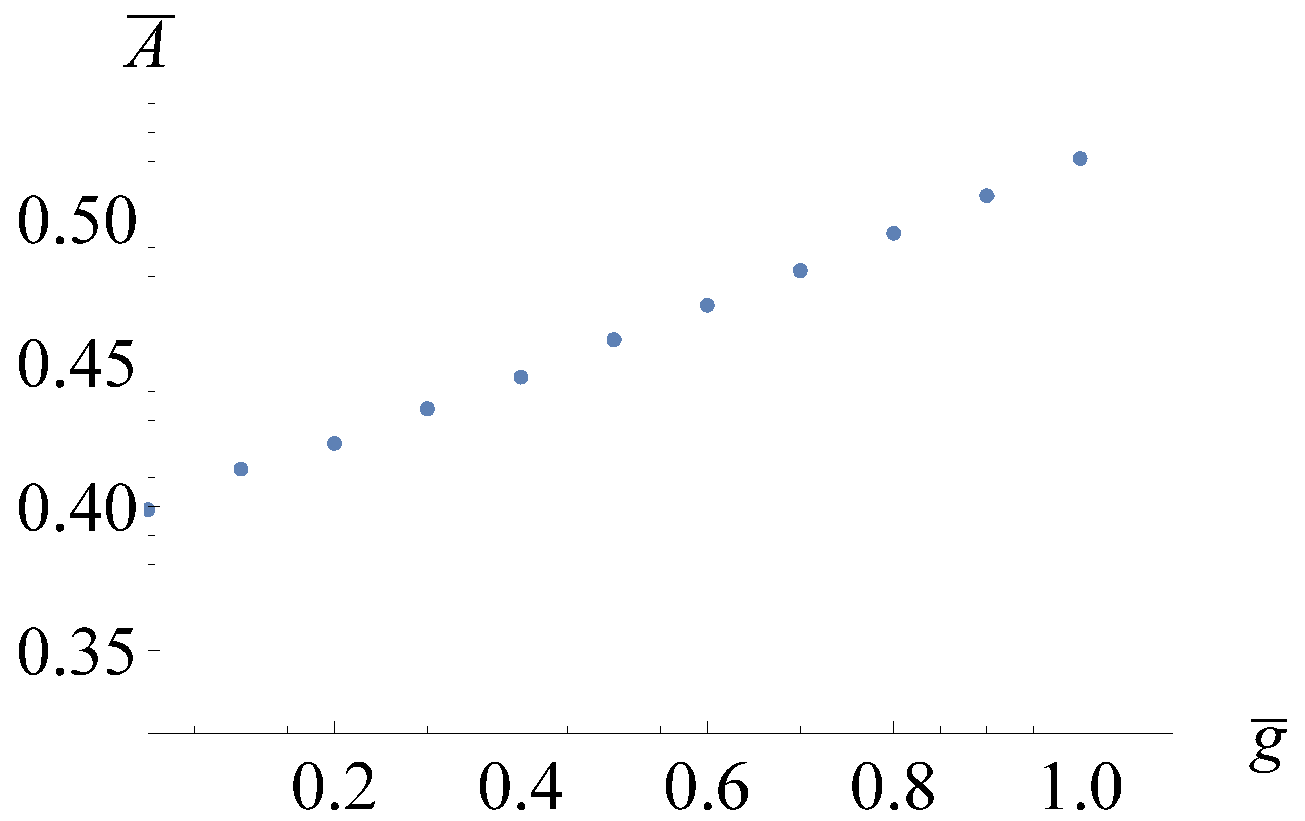
The last step concerns the determination of the normalization constant A. For instance, for the harmonic potential in Equation (5), it is convenient to introduce the rescaled variables

$$\overline{x}=\frac{x}{L},\overline{g}=\frac{N\beta g}{L},\overline{A}=\frac{A}{N\beta \omega },$$

(15)

in terms of the characteristic length $L=1/(\sqrt{\beta m}\omega )$. The normalization condition (4) yields

$$\overline{g}=\int d\overline{x}W\left[\overline{g}\overline{A}exp\left(-\frac{{\overline{x}}^2}{2}\right)\right],$$

(16)

which cannot be analytically solved for $\overline{A}$. Nevertheless, given the rescaled coupling constant $\overline{g}$ one can readily numerically obtain $\overline{A}$, as shown in Figure 1. It should be remarked that $\overline{g}$ has very small values in today’s experiments [12,31], which allows to approximate $W(s)\simeq s$ for a generic argument $s\ll 1$ in Equation (16), yielding $\overline{A}=1/\sqrt{2\pi }=0.40$ in this approximation. For instance, with $N=100,g=5\times {10}^{-41}\mathrm{kg}{\mathrm{m}}^3{\mathrm{s}}^{-2},m=9\times {10}^{-27}\mathrm{kg}$ (Li atom) as in [12] together with typical values $\omega =700\mathrm{rad}/\mathrm{s},\beta ={10}^{28}{\mathrm{J}}^{-1}$ [32,33] one has $L=0.15\mathrm{mm},\overline{g}=3.32\times {10}^{-7}$. The validity conditions (7) and (8) are safely meet for these parameters. Moreover, from Equation (6) one would need an energy of transverse confinement $\hslash {\omega }_{\perp }$ with ${\omega }_{\perp }\gg {10}^6\mathrm{rad}/\mathrm{s}$.

It is interesting to rewrite the validity condition (7) using the approximations $\overline{g}\ll 1$ and $\overline{A}\simeq 1/\sqrt{2\pi }$ so that $A\simeq N\beta \omega /\sqrt{2\pi }$. From Equation (13), one has the estimate $\rho \sim N\omega \sqrt{\beta m/(2\pi )}$. Together with $<p^2>/(2m)\sim 1/\beta$, one has that Equation (7) becomes

$$\frac{1}{\beta }\gg N\hslash \omega ,$$

(17)

which has an evident thermodynamic meaning. Under the same approximation, the Lambert function in Equation (14) can be safely replaced by $W(s)\simeq s$ so that the number density assumes the Maxwellian form

$$\rho (x)=N\omega {\left(\frac{\beta m}{2\pi }\right)}^{1/2}exp\left(-\beta V(x)\right).$$

(18)

To summarize and without any approximation within the Landau–Vlasov model, for the Maxwell–Boltzmann distribution (12) one has the exact number density (14), subject to $N=\int dx\rho (x)$ which determines the normalization constant A given an arbitrary external potential $V(x)$.

3.2. Water Bag Distribution

In a non-equilibrium situation we are free to have any function of the total energy as a suitable particle distribution function. A second example is provided by a completely degenerate Fermi–Dirac-like distribution

$$f(H)=A\mathsf{\Theta }(E_F-H),$$

(19)

where $\mathsf{\Theta }$ is the step function, A is a normalization constant, and $E_F>0$ is a energy parameter which would be the Fermi energy in a Fermi gas. Moreover, we assume $E_F\ge U(x)$; otherwise, some quantities become complex valued in the following. However, in the context of a bosonic gas, $E_F$ is just a measure of the energy spread, precisely as in the water bag model for plasmas [34]. By construction, Equation (19) shows an exact stationary solution of the Landau–Vlasov equation.

Integration in momentum space implicitly gives the 1D number density

$$\rho (x)=2A\sqrt{2m}{\left(E_F-U(x)\right)}^{1/2}.$$

(20)

Note for real $\rho$ one has $E_F\ge U(x)$ and hence automatically $E_F\ge V(x)$, supposing $g>0$ (repulsive interaction). The always non-negative solution of Equation (20) is

$$\rho (x)=4m{A}^2\left[-g+{\left(g^2+\frac{1}{2m{A}^2}(E_F-V(x)\right)}^{1/2}\right].$$

(21)

The exact total potential (11) is also immediately available, for arbitrary external potential.

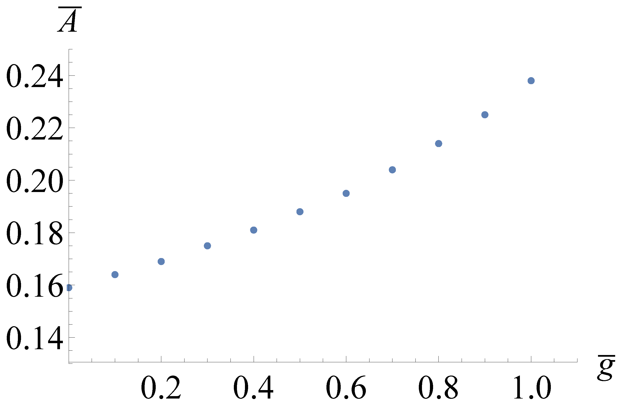
The last step is the determination of the normalization constant A, once a specific external potential is chosen. For the harmonic potential (5), it is convenient to introduce the rescaling

$$\overline{x}=\frac{x}{L},\overline{g}=\frac{Ng}{E_{F}L},\overline{A}=\frac{E_{F}A}{N\omega },\overline{\rho }=\frac{\rho }{N/L},$$

(22)

in terms of the characteristic length $L=\sqrt{E_F/m}/\omega$. The dimensionless 1D number density becomes

$$\overline{\rho }=4{\overline{A}}^2\left[-\overline{g}+{\left({\overline{g}}^2+\frac{1}{2{\overline{A}}^2}\left(1-\frac{{\overline{x}}^2}{2}\right)\right)}^{1/2}\right],$$

(23)

and the normalization condition $\int dx\rho (x)=N$ yields

$$\frac{1}{4{\overline{A}}^2}={\int }_{-\sqrt{2}}^{\sqrt{2}}d\overline{x}\left[-\overline{g}+{\left({\overline{g}}^2+\frac{1}{2{\overline{A}}^2}\left(1-\frac{{\overline{x}}^2}{2}\right)\right)}^{1/2}\right],$$

(24)

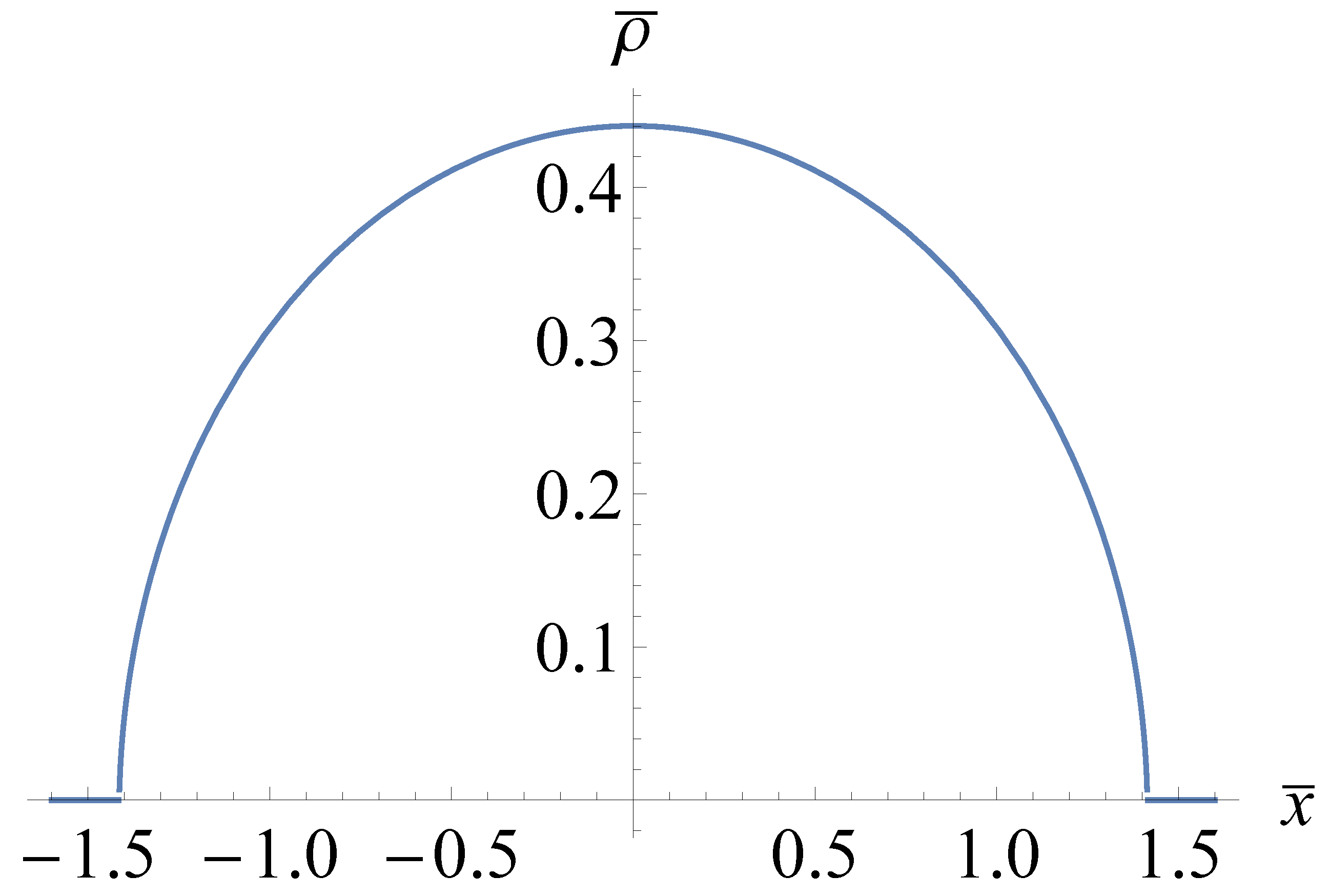
where $E_F\ge V(x)$ yields ${\overline{x}}^2\le 2$ in dimensionless variables. The integral in Equation (24) can be analytically done, but in terms of transcendental functions which are not useful to show here. For specific values of $\overline{g}$, one can numerically determine $\overline{A}$ and hence the necessary normalization, as depicted in Figure 2. In the limit of very small $\overline{g}$ one has $\overline{A}=1/(2\pi )=0.16$. The resulting dimensionless 1D number density is shown in Figure 3.

Similarly to the Maxwellian case, it is possible to rewrite the validity condition (7) using the approximations $\overline{g}\ll 1$ and $\overline{A}\simeq 1/(2\pi )$. From Equation (20) one has the estimate $\rho \sim 2A\sqrt{2m{E}_F}$. Together with $<p^2>/(2m)\sim E_F$ yields

$$E_F\gg N\hslash \omega ,$$

(25)

with an evident thermodynamic meaning.

To summarize and without any approximation within the Landau–Vlasov model, for the water bag, completely degenerate Fermi–Dirac-like distribution (19) one has the exact number density (21), subject to $N=\int dx\rho (x)$ which determines the normalization constant A given an arbitrary external potential $V(x)$. For the sake of introducing the next section, notice the correspondence between the Van Kampen mode decomposition and the water bag distribution which is shown to be granted in the limit of an infinite number of bags [35].

4. Case–Van Kampen Modes

The Case–Van Kampen modes are the normal modes in a plasma [21,22]. For the Landau–Vlasov equation, Case–Van Kampen modes can be derived starting from the assumption $V=0$. Experimentally, a 1D configuration of ultracold atoms free of external confinement can be produced by means of a 1D ring geometry with large radius [11] or considering two high barriers at the edges of a straight axial arrangement [36]. In both cases, spatial periodic conditions can be assumed. The 1D Landau–Vlasov equation reduces to

$$\left(\frac{\partial }{\partial t}+\frac{p}{m}\frac{\partial }{\partial x}-g\int d{p}^{\prime }\frac{\partial f(x,p^{\prime },t)}{\partial x}\frac{\partial }{\partial p}\right)f(x,p,t)=0,$$

(26)

To proceed, we set

$$f(x,p,t)=f_0(p)+\delta f(x,p,t),$$

(27)

where $f_0(p)$ is the equilibrium distribution subject to

$$\int dp{f}_0(p)=n_0$$

(28)

where $n_0$ is the equilibrium 1D number density and $\delta f(x,p,t)$ is a first-order perturbation. Due to the periodic boundary conditions, it is meaningful to Fourier transform according to

$$\delta f(x,p,t)=\sum _k{f}_k(p,t)e^{ikx},$$

(29)

where k is a multiple of a fundamental wavenumber. Linearizing the Landau–Vlasov Equation (26) the result is

$$\frac{\partial f_k(p,t)}{\partial t}+\frac{ikp}{m}{f}_k(p,t)-igk\frac{\partial f_0(p)}{\partial p}\int d{p}^{\prime }{f}_k(p^{\prime },t)=0.$$

(30)

Complementary to the Landau approach where the linearized Landau–Vlasov equation is taken as an initial value problem analyzed by Laplace transform methods, the Case–Van Kampen approach assumes

$$f_k(p,t)=f_{\nu }(p)e^{-i\omega t},\nu =\frac{\omega }{k},$$

(31)

where $\omega$ is a real, arbitrary constant and $\nu$ is the phase speed. Inserting from Equation (31) into Equation (30) gives the eigenvalue problem

$$\left(p-m\nu \right)f_{\nu }(p)=gm\frac{\partial f_0(p)}{\partial p}\int d{p}^{\prime }{f}_{\nu }(p^{\prime }).$$

(32)

Following [21,22], it is convenient to assume the normalization

$$\int dp{f}_{\nu }(p)=\mathrm{cte}.=n_0,$$

(33)

So that the integral Equation (32) simplifies to

$$\left(p-m\nu \right)f_{\nu }(p)=gm{n}_0\frac{\partial f_0(p)}{\partial p}.$$

(34)

In a distributional sense, the solution for Equation (34) is

$$f_{\nu }(p)=gm{n}_0\wp \left(\frac{\partial f_0(p)}{\partial p}\frac{1}{p-m\nu }\right)+\lambda (\nu )\delta \left(p-m\nu \right),$$

(35)

where ℘ denotes the Cauchy principal value symbol, $\lambda (\nu )$ is a function to be determined and where $\delta$ is the Dirac delta.

As can be readily verified, the naive solution (without principal value and with $\lambda (\nu )=0$) can not be made compatible with the normalization (33). Indeed, to comply with the normalization one needs

$$\lambda (\nu )=n_0-gm{n}_0\wp \int dp\frac{\partial f_0(p)}{\partial p}\frac{1}{p-m\nu },$$

(36)

where the integral is taken in the principal value sense. The final result is

$$\begin{array}{ccc}\hfill f_{\nu }(p)& =& gm{n}_0\wp \left(\frac{\partial f_0(p)}{\partial p}\frac{1}{p-m\nu }\right)+\hfill \\ & +& \left(n_0-gm{n}_0\wp \int d{p}^{\prime }\frac{\partial f_0(p^{\prime })}{\partial p^{\prime }}\frac{1}{p^{\prime }-m\nu }\right)\delta \left(p-m\nu \right).\hfill \end{array}$$

(37)

As apparent, these Case–Van Kampen modes are not damped (they are stationary waves) and have a singular character. Following Case, by means of the introduction of adequate adjoint solutions, it is possible to demonstrate that the Equation (37) provides a complete set, in the sense that all solutions to the linearized Landau–Vlasov equation can be expressible as a linear combination of these modes. More precisely, for simplicity we have discussed only the class 1a among the four classes of eigenfunctions in Case’s terminology, as detailed in the original article [22] and textbooks [37]. To demonstrate the completeness of the full set of Case–Van Kampen eigenfunctions makes necessary to introduce an auxiliary (or adjoint) equation with a different set of eigenfunctions, orthogonal to those in the original set, except when the eigenvalues coincide. The complete analysis is not trivial but entirely similar to the Vlasov–Poisson case, shown in [22,37], for instance.

Note that in spite of the singular character of the Case–Van Kampen modes, they can be used to compute well behaved physical quantities. For instance, we can consider the 1D number density perturbation

$$\delta n(x,t)=\int dpdwc(\omega )\delta f(x,p,t),$$

(38)

where $c(\omega )$ is an arbitrary weight function. Allowing a superposition law taking into account a frequency spread is valid in the context of the linearized Landau–Vlasov equation. Restricting to the k-th Fourier component, applying Equations (31) and (37), we have the well behaved function

$$\delta n(x,t)=\frac{n_{0}k}{m}\int dpc\left(\omega =\frac{kp}{m}\right)e^{ik(x-\frac{pt}{m})},$$

(39)

after using the property $\delta (p-m\omega /k)=(k/m)\delta (\omega -kp/m)$. In this case, the first and last terms of Equation (37) cancel upon integration (the same occurs for Vlasov–Poisson plasmas [37]).

As a simple illustration, the Gaussian weight function

$$c(\omega )=\frac{\delta n_0}{\sqrt{2\pi }\mathsf{\Omega }{n}_0}exp\left(-\frac{{(\omega -{\omega }_0)}^2}{2{\mathsf{\Omega }}^2}\right)$$

(40)

produces from integration of Equation (39) the density perturbation

$$\delta n(x,t)=\delta n_{0}exp\left(i(kx-{\omega }_{0}t)-\frac{{\mathsf{\Omega }}^2{t}^2}{2}\right).$$

(41)

This is an example of the well known fact that although the isolated Case–Van Kampen eigenmodes are stationary waves, they can produce damped macroscopic objects, taking into account phase mixing. Consistently, the monochromatic limit $\mathsf{\Omega }\to 0$ is not damped.

5. Conclusions

In the context of mean-field collisionless theory for 1D ultracold dilute Bose gases, non-decaying nor growing in time structures have been analyzed. For this purpose, traditional methods from plasma theory have been adapted to the Landau–Vlasov equation. Nonlinear stationary solutions have been derived in analogy with the BGK modes of the Vlasov–Poisson system in plasmas. Specific kinetic equilibria have been worked out in detail, together with the associated validity conditions in real ultracold bosonic gases. Linear, normal modes have been also derived, in analogy with the plasma Case–Van Kampen stationary wave modes. These results are a necessary complementary development to the analysis of Landau damping and instabilities for the 1D Landau–Vlasov equation [12]. The stability of the BGK modes for the Landau–Vlasov equation is an important point to be addressed in future works.