Quasi-Static and Dynamic Photon Bubbles in Cold Atom Clouds

Abstract

Turbulent radiation flow is ubiquitous in many physical systems where light–matter interaction becomes relevant. Photon bubble instabilities, in particular, have been identified as a possible source of turbulent radiation transport in astrophysical objects such as massive stars and black hole accretion disks. Here, we report on the experimental observation of a photon bubble instability in cold atomic gases, in the presence of multiple scattering of light. Two different regimes are identified, namely, the growth and formation of quasi-static structures of depleted atom density and increased photon number, akin to photon bubbles in astrophysical objects, and the destabilisation of these structures in a second regime of photon bubble turbulence. A two-fluid theory is developed to model the coupled atom–photon gas and to describe both the saturation of the instability in the regime of quasi-static bubbles and the low-frequency turbulent phase associated with the growth and collapse of photon bubbles inside the atomic sample. We also employ statistical dimensionality reduction techniques to describe the low-dimensional nature of the turbulent regime. The experimental results reported here, along with the theoretical model we have developed, may shed light on analogue photon bubble instabilities in astrophysical scenarios. Our findings are consistent with recent analyses based on spatially resolved pump–probe measurements.

1. Introduction

Due to multiple scattering of light in dense astrophysical systems such as massive stars [1], black hole accretion disks [2,3], or the atmosphere of neutron stars [4], light transport is often diffusive instead of ballistic. In such optically thick media, photons exhibit high residence times and can therefore be trapped. One interesting consequence of this diffusive behaviour is the so-called photon bubbling effect, expected when matter strongly responds to the propagation of light. Photon bubbling consists in the formation and growth of light bubbles that eventually leave the medium or decay into smaller structures. This decay is at the origin of a specific form of turbulence in optically thick media, photon bubble turbulence (PBT). Novel forms of turbulence can therefore be investigated in systems with strong light–matter coupling, where the turbulent character of light transport strongly depends on the optical properties of the medium [5]. The observation of photon bubbling turbulence in cold atomic gases has recently been reported by some of us [6]. The spatial pattern of the complex turbulent dynamics has been investigated by means of a spatially resolved pump–probe technique, which allows for the retrieval of an instantaneous direct image of the atomic density distribution across the cold atom cloud. The measured atomic local structure, averaged over numerous system realisations, is dominated by quasi-coherent structures which have been associated to fully developed photon bubbles whose growth and subsequent collapse has been proposed as the driving mechanism of the identified turbulent regime. In analogy to its astrophysical counterpart, PBT in cold atom gases arises as radiation pressure becomes comparable to thermal pressure. The strength of the light–matter interaction can be effectively increased by driving the cold atom cloud close to the electronic resonance: as the atomic medium becomes optically thick, radiation propagation turns diffusive, inducing a fluid-dynamic instability which is at the root of PBT.

Here, the atomic density distribution is probed by collecting the line-of-sight integrated fluorescence signal, which allows for studying the real-time dynamical evolution of the system [5,7,8]. We start by revising the theoretical model describing the dynamics of the coupled atom–light gases and revealing the mechanism of the photon bubble instability. The experimental results are then presented, with two distinct regimes being identified. On the one hand, quasi-static radiation-filled regimes resulting from the saturation of the instability are described; on the other hand, at higher values of optical thickness, these structures tend to grow beyond the limit that the cold atomic gas is able to sustain, causing the collapse (or burst) of the bubble and resulting in a distinct form of turbulence, accurately described by the theoretical model in the form of dynamical spherical bubbles. To further characterise the turbulent regime, we apply data-driven (model independent) dimensionality reduction techniques—principal component analysis—in order to find a low-dimensional representation of turbulence, whose results are shown to be in agreement with the theoretical description in terms of the photon bubble mechanism.

2. Theoretical Model

Atomic clouds comprised of high numbers of atoms, and when driven close to electronic resonances, are optically thick. As a result, photons are scattered multiple times, undergoing a random walk inside the cloud. Such processes are described by a diffusion equation for the light intensity distribution I, namely [5,6,9,10]:

$$\frac{\partial }{\partial t}I-\nabla ·\left(D\nabla I\right)=0.$$

(1)

The diffusion coefficient $D=l^2/\tau$ quantifies photon transport, with $l=1/n{\sigma }_L$ denoting the photon mean free path, n the atom density, and ${\sigma }_L$ the photon absorption cross-section. The interval between consecutive scattering events determines the photon diffusion time $\tau$. The latter is approximately given by the lifetime of the excited state, $\tau \simeq 1/\Gamma$, with $\Gamma$ being the transition linewidth [7]. The coupling between the atom dynamics and photon transport originates from the dependence of the diffusion coefficient on the local density of atoms, namely, $D\propto n^{-2}$.

Assuming local hydrodynamical equilibrium, the atom density n and velocity field $\mathbf{v}$ are modelled with the usual continuity and Navier–Stokes equations:

$$\frac{\partial n}{\partial t}+\nabla ·\left(n\mathbf{v}\right)=0\mathrm{and}$$

(2)

$$\frac{\partial \mathbf{v}}{\partial t}+(\mathbf{v}·\nabla )\mathbf{v}=\frac{\mathbf{F}}{m}-\frac{\nabla P}{nm}-\nu \mathbf{v},$$

(3)

with $P=n{k}_{B}T$ being the equation of state of an ideal gas, $\nu$ the optical damping rate (optical molasses), and m the atom mass. The exchange of photons between nearby atoms and the associated momentum recoil is also at the origin of a repulsive radiation pressure force $\mathbf{F}$, scaling as $1/r^2$ and determined by the mean-field Poisson equation:

$$\nabla ·\mathbf{F}=Qn,$$

(4)

where $Q=({\sigma }_R-{\sigma }_L){\sigma }_{L}I/c$ is the effective charge, with ${\sigma }_R$ denoting the absorption cross-section for re-scattered photons [11,12]. An effective plasma frequency, ${\omega }_p=\sqrt{Q{n}_0/m}$ [13], immediately follows and allows for analogies with one-component trapped plasmas [8]. In typical experimental conditions, the effective charge is of the order $q=\sqrt{{ϵ}_{0}Q}$∼${10}^{-4}e$, with e being the electron charge, and $n_0$∼${10}^{10}$${\mathrm{cm}}^{-3}$ the typical atom density, resulting in a plasma frequency of ${\omega }_p/2\pi$∼50–200 Hz [14,15]. Notice that Q depends on the light intensity I, providing additional coupling between the atom and photon dynamics.

The previous coupling can, in specific conditions, become unstable, leading to the nucleation of photon bubbles—a local increase in the photon number accompanied by a depletion in the atom density [5]. The linear growth rate of the instability is given by:

$${\Gamma }_{\beta }=-\frac{\nu }{2}-\frac{\beta }{{\omega }^2\left(k\right)}.$$

(5)

Here, ${\omega }^2\left(k\right)={\omega }_p^2+u_s^2{k}^2+D_0^2{k}^4$ is the dispersion relation of the coupled atom–light gases, with k being the perturbation wavenumber. The coupling coefficient $\beta =D_0{\omega }_p^2\frac{{\nabla }^2{I}_0}{I_0}$ depends on both the initial (equilibrium) diffusion coefficient $D_0$, and the light distribution $I_0$. The finite temperature of the atoms yields the thermal speed of sound $u_s=k_{B}T/m$. From the growth rate in Equation (5), the crossing of the instability threshold (${\Gamma }_{\beta }>0$) requires the following conditions to be satisfied:

$$\beta <0\mathrm{and}\frac{2\left|\beta \right|}{{\omega }^2\left(k\right)}>\nu ,$$

(6)

which, from the first relation, depend on initial local inhomogeneities in the photon distribution $I_0$. Note that the photon bubble mechanism differs from the pattern formation instability in cold atoms [16]. In the latter, optical dipole forces, originating from far-off-resonant light and resulting from the conversion of light phase fluctuations into amplitude modulations, act on the atoms and trigger an instability in the transverse plane of the laser, whereas here we rely on quasi-resonant radiation pressure. Moreover, the pattern formation instability results from coherent photon transport, while here light is in the diffusive limit. Moreover, in contrast with the similar astrophysical instabilities, the photon bubble mechanism reported here does not require the presence of magnetic fields.

3. Experimental Results

We prepare an atomic sample of cooled ${}^{85}$Rb atoms in a magneto-optical trap (MOT) [17]. In a typical sample, we obtain up to N∼${10}^9$ atoms at T∼200 $\mathsf{\mu }$K and a maximum density $n_0$∼${10}^{10}$${\mathrm{cm}}^{-3}$ in a near spherical cloud of about 4 mm in diameter. All the experiments are conducted with a magnetic field gradient of $\nabla B$∼9 G/cm. While the magnetic field has no significant influence on the observed effects, the laser detuning $\delta$ strongly determines the stability of the system through the cross-sections ${\sigma }_L$ and ${\sigma }_R$ [14]. Within the two-level atom approximation, and in the high-intensity limit relevant for our experiments ($I\gtrsim I_{\mathrm{sat}}$, with $I_{\mathrm{sat}}\simeq 1.4$$\mathrm{mW}/{\mathrm{cm}}^{-2}$), the plasma frequency scales as ${\omega }_p$∼${\left|\delta \right|}^{-2}$, away from the resonance, $\left|\delta \right|\gg \Gamma$ [12,14]. However, close to the resonance, $\left|\delta \right|$∼$\Gamma$, complications due to the Zeeman splitting of the excited manifold arise, rendering the two-level atom approximation invalid. In any case, we use $\delta$ as the relevant experimental parameter, sweeping the different regions of the stability diagram. In the first part of the experiment, the trap is loaded by switching on the laser beams and the magnetic field gradient for a total duration of 3 s, long enough to ensure a steady-state number of atoms. The laser detuning during the loading step is fixed at ${\delta }_{\mathrm{load}}=$$-3\Gamma$. It is then shifted to a different value ${\delta }_{\exp }$ for a duration of 2 s, long enough so that the photon bubble instability is fully saturated and the density reaches a steady-state distribution. We then release the trap by turning off the magnetic field gradient and the trapping light. After a transient time of approximately 200 $\mathsf{\mu }$s (to ensure the absence of any residual B field during the imaging sequence), we illuminate the trap with far-off-resonant light (${\delta }_{\mathrm{imag}}=-4\Gamma$) and collect the atomic fluorescence signal with a CCD camera during an exposure time of about 300 $\mathsf{\mu }$s. As we shall demonstrate later, with ${\delta }_{\mathrm{imag}}=-4\Gamma$, the imaging occurs in the single-scattering regime, thus ensuring the correct retrieval of the column density distribution, a crucial feature for the subsequent interpretation of the experimental results. For each value of ${\delta }_{\exp }$, we repeat the loading and imaging sequence 255 times. The entire process is then repeated for different values of ${\delta }_{\exp }$, the parameter used to span the different instability regimes (for simplicity, the detuning ${\delta }_{\exp }$ will be referred to as $\delta$ from now on). Two additional CCD cameras, placed at orthogonal directions, allow us to monitor the overall shape and symmetry of the atomic sample.

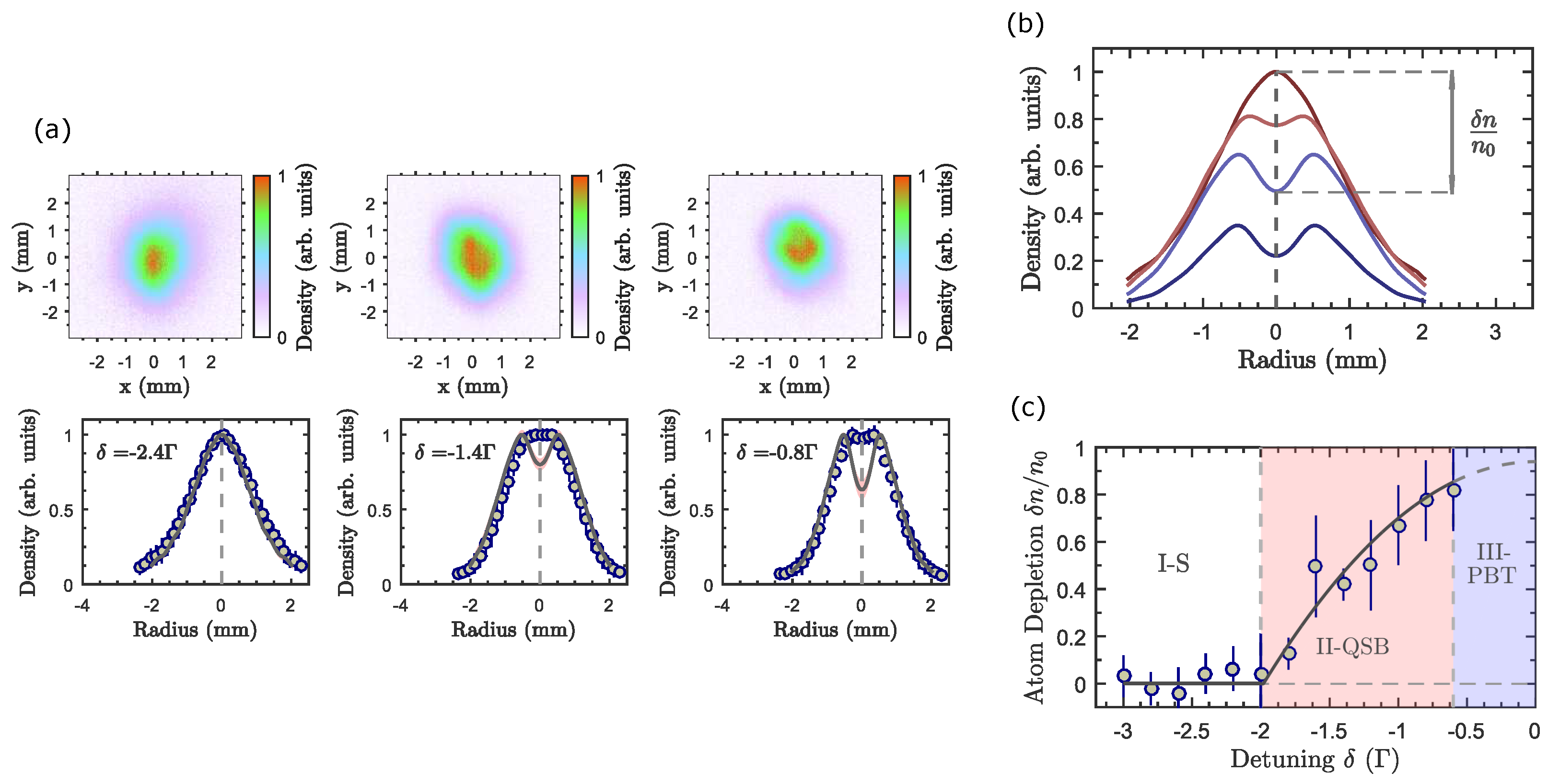
Starting from lower values of $\delta$ and going further into resonance, we observe the transition from a stable phase, persistent for $\delta \lesssim$$-2\Gamma$ and previously investigated in [15], into a regime where the photon bubble instability is triggered—see Figure 1. Note that, while the use of the laser intensity as a control parameter is mainly relevant in setting the number of atoms in the trap [11,15], the detuning from resonance is the appropriate knob to probe the different dynamical regimes [14]. To diagnose the instability, we perform fluorescence imaging on the atomic sample to retrieve the column density distribution of the trap, which, in the case of near-spherical symmetry, contains the full information about the real atom density profile. The latter is obtained by computing the inverse Abel transform, as described in Appendix A.

From the onset of the instability, a localised central region of strong radiation trapping grows. At the same time, such an increase in the local photon density is responsible for atom expulsion due to radiation pressure forces—a single photon bubble is formed at the centre of the atomic sample. As the atoms are scattered away from the centre of the bubble, the light diffusion coefficient increases due to a depleted medium. At some point, the increased diffusion losses inhibit any further growth, corresponding to the saturation of the instability as the photon bubble reaches its final state. We begin by noticing that, under near-saturation conditions, the diffusion term $D_0{k}^2$ in Equation (5) dominates over both the effective plasma frequency ${\omega }_p$ and thermal dispersion $u_{s}k$. Saturation occurs when growth is no longer sustainable due to a depleted medium and the consequent increase in photon losses, at which point the growth rate vanishes. This limit can be described as ${\omega }_p^2{L}^2/D_s=\nu /2$, with $D_s$ being the diffusion coefficient at saturation level. Here, we have also defined $\left|\frac{{\nabla }^2{I}_s}{I_s}\right|\simeq k^2\simeq L^{-2}$, with $I_s$ and L being the final photon density distribution and size of the bubble, respectively. The saturated diffusion coefficient can be written as a correction to the initial value $D_0$, due to a depletion of the atomic density $\delta n$ (with $\delta n>0$), such that $D_s=\frac{D_0{n}_0^2}{{\left(n_0-\delta n\right)}^2}$. Putting all this together, we arrive at the atomic density depletion fraction:

$$\frac{\delta n}{n_0}=1-\frac{1}{{\omega }_{p}L}{\left(\frac{\nu D_0}{2}\right)}^{1/2}.$$

(7)

Since the diffusion coefficient has always a finite value, total atomic depletion should not be expected in any situation. Recall that the diffusion coefficient is given by $D=l^2/\tau$, with $l=1/n{\sigma }_L$ being the photon mean free path. The photon scattering cross-section is determined by ${\sigma }_L=\frac{{\sigma }_0}{1+4{\left(\delta /\Gamma \right)}^2}$, with ${\sigma }_0=g3{\lambda }^2/\left(2\pi \right)$ being the on-resonance cross-section and g being a degeneracy factor that depends on the specific atomic transition [18]. We can then rewrite Equation (7) in terms of the photon detuning $\delta$ as:

$$\frac{\delta n}{n_0}=1-\frac{1}{{\omega }_{p}L}{\left(\frac{\nu D_0^r}{2}\right)}^{1/2}\left[1+4{\left(\delta /\Gamma \right)}^2\right],$$

(8)

with $D_0^r=1/\tau n_0^2{\sigma }_0^2$ being the diffusion coefficient at resonance. This relation can be fitted to the experimental results—see Figure 1—which correctly describes both the onset, the unstable phase at $\delta \simeq$$-2\Gamma$, and the final state of instability in the form of quasi-static photon bubbles (QSB).

At this point, we shall elucidate the validity of the diffusion approximation in Equation (1). The photon mean free path has been carefully measured to be of the order of ${\ell }_0=$ 300 $\mathsf{\mu }$m for resonant light [7]. For $\delta =-0.8\Gamma$, where a high depletion fraction is observed, we estimate $\ell ={\ell }_0[1+4{\left(\delta /\Gamma \right)}^2]$∼700 $\mathsf{\mu }$m and, thus, $\ell \ll w$, with w∼4 mm being the diameter of the atomic sample, thereby ensuing the validity of the diffusion approximation. Moreover, and to further consolidate the experimental observations as evidence of photon bubbles, notice that their spatial extent is expected to be of the order ℓ, namely, $L\gtrsim \ell$, in good agreement with the structures depicted in Figure 1. In addition, for ${\delta }_{\mathrm{imag}}=$$-4\Gamma$, one obtains ℓ∼20 mm, thus ensuring the single-scattering regime during the imaging sequence.

The atom density profiles observed in the QSB regime, which persist approximately for $\delta \lesssim$$-0.6\Gamma$, are not described by the usual Wieman model [11], which predicts a flattened density in the case of moderate optical thickness and does not account for the effects associated with the diffusive nature of light. For smaller values of $\left|\delta \right|$ (i.e., closer to resonance), a dramatic change of the dynamics of the coupled atom–light gases is observed. In this regime, the instability leads to the growth of structures beyond the limit that is sustainable for the depleted atomic medium. At this point, the central photon bubble collapses, or bursts, followed by a re-establishment of the local atom density that again re-triggers the instability. Such processes are at the origin of a low-frequency turbulent regime, the photon bubble turbulence (PBT), which we shall now describe in greater detail.

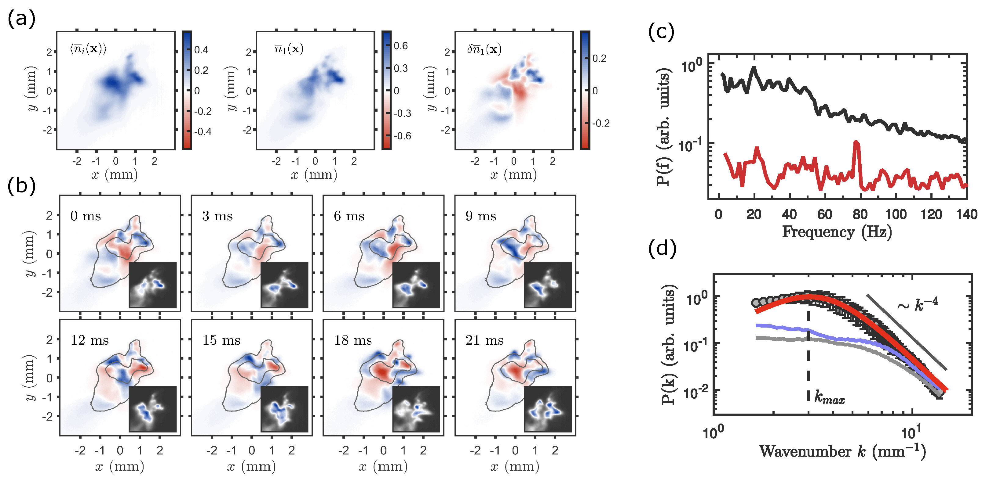
We investigate the PBT regime by bringing the driving beams very close to the atomic resonance, typically $\delta =-0.5\Gamma$. A CCD camera working at 350 fps collects the fluorescence signal from the trap, resolving the spatio-temporal properties of the turbulent regime—see Figure 2. We begin to investigate the low-frequency nature of turbulence by measuring the frequency power spectrum of the spatially resolved fluorescence time signal—see Figure 2. The total signal is nearly constant, corresponding to an approximately fixed number of atoms in the trap. Additionally, for a lower laser detuning, $\delta =$$-1.5\Gamma$ (QSB regime), low-amplitude isolated frequency peaks are observed. It has previously been described that, in a similar region of experimental parameters, the atomic cloud undergoes a supercritical Hopf bifurcation into an unstable regime of large-amplitude self-sustained oscillations [14]. In that case, nevertheless, the instability is expected for clouds with large radii, typically greater than 4 mm, and with a number of atoms of the order of ${10}^{10}$, features which safely distinguish it from the one reported here. Moreover, the unstable behaviour in Ref. [14] originates at the edge of the cloud, while the photon bubble instability is triggered in its central region. Regardless, the same authors also describe the transition from over-damped to under-damped behaviour prior to the instability threshold (lower number of atoms), which is consistent with the low-amplitude breathing oscillations of the bubbles and the red line spectrum in Figure 2. When tuning the beams closer to resonance ($\delta =$$-0.5\Gamma$), a complex dynamical regime takes place—black line in Figure 2—with the frequency spectrum exhibiting broad-band components at low frequencies, as expected in dissipative weak turbulent systems [19] and originating from the complex dynamics associated with the growth and collapse of (dynamical) photon bubbles, as we shall demonstrate.

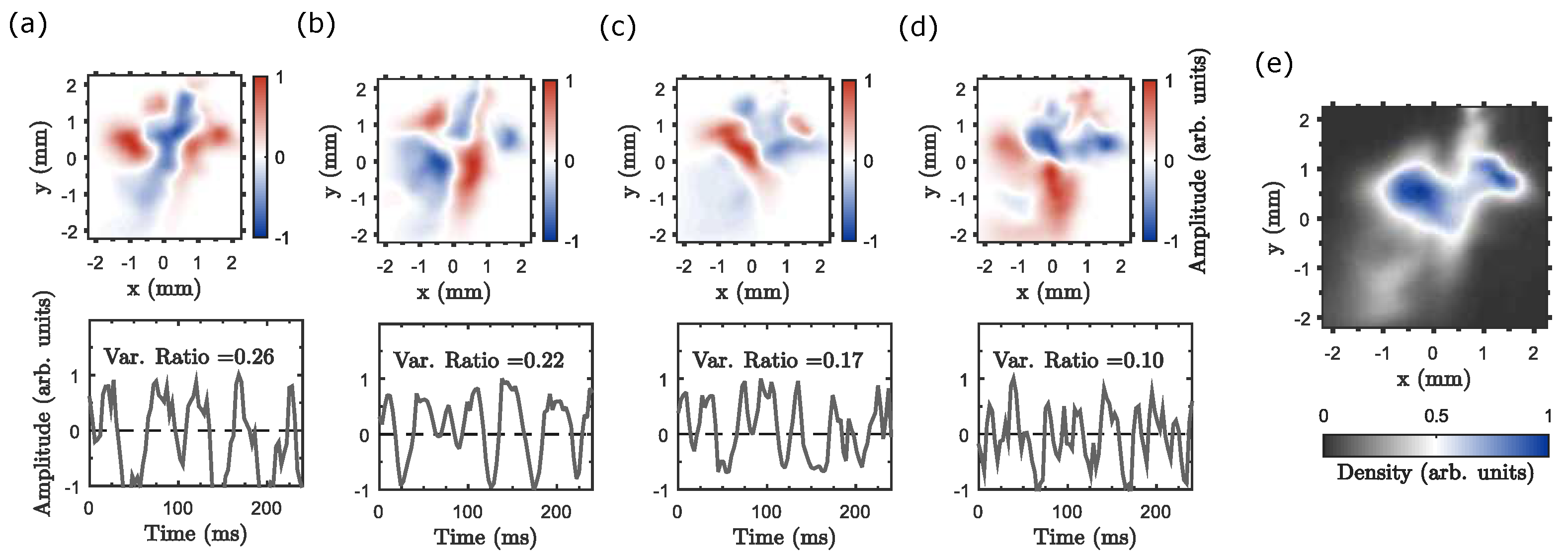
We now turn to the spatial power spectrum of the atom density fluctuations—see Figure 2—as described in detail in Appendix B. In the fully developed case ($\delta =-0.5\Gamma$), the fast $k^{-4}$ decay at high wavenumbers indicates the existence of quasi-coherent structures with well-defined scale lengths, and not self-similar (fractal) structures at different scales. This is easily understood in terms of the auto-correlation function, the conjugate quantity of the power spectrum, defined as $C\left(\delta r\right)=\langle n\left(r\right)n(r+\delta r)\rangle$. For a scaling of the form $P\left(k\right)$∼$1/{(a^2+k^2)}^2$, similar to a squared Lorentzian function, such as we experimentally observe, where a is a regularisation at $k\to 0$ (related with the inverse of the typical scale), the auto-correlation function takes the form $C\left(\delta r\right)$∼$\exp (-a\delta r)$, evidencing the existence of well-defined spatial structures of typical size a (photon bubbles).

In order to make the above phenomenological arguments more accurate, we shall at this point resort to the photon bubble model. From the fluid equations, we derive the power spectrum of the density fluctuations (of both the atom and light gases) and in the case of dynamical spherical bubbles as $P\left(k\right)=4\pi k^2{\left|S_0\left(k\right)\right|}^2$:

$$S_0\left(k\right)=\frac{8\pi \left(\gamma -ik\right)}{{[k_a^2+{(\gamma -ik)}^2]}^2},$$

(9)

as derived in Appendix C. Here, $k_a$ essentially defines the inverse of the bubble size and, for $k\gg k_a$, the spectrum decays as $k^{-4}$, as observed in the experiment. To further clarify the consistency of the model, we numerically fitted the theoretical power spectrum to the experimental results—see Figure 2—where a good agreement is observed. The spectrum attains its maximum near $k_{\max }$∼$k_a$∼3 mm${}^{-1}$, corresponding to the typical bubble length $l_0$∼$2\pi /k_a$∼2 mm. For lower wavenumbers $k\lesssim k_{\max }$, the theoretical curve slightly diverges from the experimental data. This may be attributed to finite-size effects, given that the typical bubble size is just slightly smaller than the diameter of the system (about 4 mm). The $k^{-4}$ decay observed here is close to the Kolmogorov scaling, which, in the case of homogeneous and isotropic turbulence, gives a $k^{-11/3}$ inertial range in the spectrum of density fluctuations. As we have shown, however, and despite the closeness with the Kolmogorov scaling, the spectrum observed here is of a distinct physical origin, related to the complex dynamics associated with the growth and collapse of photon bubbles. The observations reported here are compatible with the ones in Ref. [6], where the quasi-coherent structures—emerging from a realisation-average procedure—have been successfully associated to a fully developed photon bubble turbulence regime. Here, we recover the same spatial local structure, and we investigate the full dynamical evolution of the system. Moreover, unlike what has been reported in [6], where a sharp transition from a stable to a turbulent regime had been observed, here, the transition into the fully developed phase is continuous—see Figure 2. Nevertheless, the fully turbulent phase is only observable in a narrow range of experimental parameters. For $\delta >-0.4\Gamma$, for instance, the number of atoms in the trap is significantly lower, reducing the overall optical thickness and strongly suppressing the diffusive nature of light.

Regarding the low-frequency nature of the turbulent regime, we can inquire about the temporal dynamical scale associated with the inverse of the typical bubble length, $k_{\max }$. Going back to Equation (5), and considering a temperature $T=$ 200 $\mathsf{\mu }$K, ${\omega }_p$∼$2\pi \times$ 100 s${}^{-1}$ and a diffusion coefficient at resonance of $D_0^r$∼$0.5$ m${}^2$/s [7], we can compute the corresponding growth rate ${\Gamma }_{\beta }$∼10 s${}^{-1}$. Here, we also used the condition that the damping term $\nu$ from the optical molasses is not the dominant term at the centre of the cloud, corresponding to the region where the bubble nucleates, and that the initial perturbations of the light intensity distribution occur at a scale much smaller than the final bubble size, namely, $|{\nabla }^2{I}_0|/I_0\gg k_{\max }^2$. The initially fast instability growth is gradually reduced as the light intensity increases and the atom density decreases during the bubble growth. As such, slower time scales are associated with higher energies (larger structures), which is at the origin of the observed (temporal) power spectrum. The same instability mechanism is at the origin of both the previously reported regime of quasi-static photon bubbles (QSB) and the turbulent (PBT) phase. In summary, strong radiation trapping affects the collective atomic dynamics and leads to the growth of photon bubbles. While in the QSB phase, the atomic medium is able the support the saturation of the instability, in the PTB regime, photon losses due to the depleted medium lead to the burst and decay of the bubbles, with such continuous processes being at the origin of the low-frequency turbulent regime described here.

4. Normal Modes and Low-Dimensional Turbulence

The origin of the PBT regime in the growth and collapse of photon bubbles points towards a weak, low-dimensional form of turbulence. Turbulent flow is considered, in general, an infinite dimensional process, as described by some set of nonlinear partial differential equations—usually, the fluid equations introduced before or some simplification of them [20,21,22]. In some physical systems, however, the existence of coherent spatial structures, interacting nonlinearly with each other, allows for the description of turbulence in terms of finite or even low-dimensional processes [23,24]. The Lorenz model of atmospheric convection [25] or the Couette–Taylor flow [26] are canonical examples where turbulence is effectively described as a dynamical system in a low-dimensional space, often exhibiting chaos and the existence of strange attractors governing their evolution [27,28]. To further clarify the low-dimensional character of the photon bubble turbulence, we now turn to a rather different approach. Advancements in machine learning and data science [29,30] have been providing different ways to tackle and retrieve useful information from complex data. Here, we apply the technique of principal component analysis (PCA) [31] to retrieve the coherent structures or normal modes of the PBT regime, if they exist. This approach can be cast inside the more general discipline of dimensionality reduction [32], with the purpose of finding a low-dimensional representation of a given (higher-dimensional) dataset, written as a linear combination of state vectors (the principal components), chosen in such a way that they are statistically uncorrelated with each other. Each component can then be identified with a particular dynamical process, such as atom number fluctuation, centre-of-mass motion, trap modes of oscillation, etc. We stress that PCA is a model-free approach, requiring no assumption of the physical nature of the underlying dynamics. The validity of the PCA technique to extract the collective normal modes has been confirmed with numerical simulations of the Gross–Pitaevskii equation for Bose–Einstein condensates [33]. Moreover, it has been recently used to diagnose some class of spatial instabilities in clouds of cold atoms [34].

The results obtained from PCA on the turbulent regime are depicted in Figure 3—further details on PCA technique can be found in Appendix D. The first mode (highest variance ratio) determines the growth of the central region of strong radiation trapping, together with the corresponding depletion of atoms as they are pushed outwards by radiation pressure forces. The slight asymmetry shown here follows from the asymmetries of the trapping potential. The second mode, accounting for 0.22 of the total data variance, entails a collective trap mode, bearing similarities with a quadrupolar structure. The third and fourth principal components depict a compression mode and fluctuations in the centre-of-mass (COM) position of the cloud, respectively, with the axes of both aligned with the direction of strong trapping. The evolution of the fourth mode accounting for COM drift is essentially decoupled from the remaining dynamics, resulting from fluctuations in both the polarisation and power of the trapping beams. In the same way, the remaining principal components (not shown here) represent mostly noise in the COM position in the remaining directions and in the total number of atoms. Altogether, the first three modes correspond to approximately 0.65 of the total dynamics observed in the PBT regime, with the remaining components representing mostly noisy processes decoupled from the main evolution. The nontrivial time evolution may indicate the existence of complex nonlinear coupling among such dynamical modes. Moreover, the principal component analysis decomposition represents a step forward towards the reconstruction of the phase space associated with the turbulent phase. Here, the state variables may be represented by each of the normal modes, with the phase space trajectories defined by their corresponding time evolution, in a manner analogous to the Lorenz model of atmospheric convection. The investigation of these trajectories may provide deep insight into the nature of the turbulent regime.

5. Conclusions

In this paper we have studied, through the collection of fluorescence light, the atomic spatio-temporal dynamics arising from the cold atom photon bubble instability. This instability stems from the strong coupling between diffusive light and atomic matter and results in the growth of local pockets of high radiation intensity and low atomic density—photon bubbles. A new regime has been identified, namely, the quasi-static bubble regime. This is characterised by the formation, at the centre of the cloud, of a stable weakly oscillating single bubble which arises from the saturation of the photon bubble instability, due to the photon diffusion losses through the depleted medium. For close-to-resonance driving, the bubble grows beyond the limit sustainable for the atomic cloud. Hence, the bubble bursts and decays into smaller structures, causing the atomic density to be restored and, thus, re-triggering the instability. This phenomenon is known as photon bubble turbulence. In this manuscript, we have described its low-frequency behaviour, associating it to the dynamics of large photon bubbles. We have, therefore, unified the interpretation of the quasi-stationary and turbulent regimes as originating from the same photon bubble instability. We also provided additional evidence pointing towards the low-dimensional nature of the PBT regime, based on a dimensionality reduction approach to the experimental data. Further investigations may be conducted towards the reconstruction of the phase space trajectories. The existence of strange attractors and/or chaos governing the dynamics associated with photon bubble turbulence are exciting possibilities, offering an interesting new platform to study some fundamental problems of low-dimensional turbulence, dynamical systems, and chaos, where the huge gap between the many theoretical developments and the elusive experimental observations has yet to be bridged.

References

1. Turner, N.J.; Quataert, E.; Yorke, H.W. Photon Bubbles in the Circumstellar Envelopes of Young Massive Stars. Astrophys. J. 2007, 662, 1052. [Google Scholar] [CrossRef]
2. Gammie, C.F. Photon bubbles in accretion discs. Mon. Not. R. Astron. Soc. 1998, 297, 929. [Google Scholar] [CrossRef] [Green Version]
3. Begelman, M.C. Photon Bubbles and the Vertical Structure of Accretion Disks. Astrophys. J. 2006, 643, 1065. [Google Scholar] [CrossRef] [Green Version]
4. Arons, J. Photon bubbles—Overstability in a magnetized atmosphere. Astrophys. J. 1992, 388, 561–578. [Google Scholar] [CrossRef]
5. Mendonça, J.T.; Kaiser, R. Photon Bubbles in Ultracold Matter. Phys. Rev. Lett. 2012, 108, 033001. [Google Scholar] [CrossRef]
6. Giampaoli, R.; Rodrigues, J.D.; Rodrigues, J.A.; Mendonça, J.T. Photon bubble turbulence in cold atom gases. Nat. Commun. 2021, 12, 3240. [Google Scholar] [CrossRef]
7. Labeyrie, G.; Vaujour, E.; Müller, C.A.; Delande, D.; Miniatura, C.; Wilkowski, D.; Kaiser, R. Slow Diffusion of Light in a Cold Atomic Cloud. Phys. Rev. Lett. 2003, 91, 223904. [Google Scholar] [CrossRef] [Green Version]
8. Mendonça, J.T.; Terças, H. Physics of Ultra-Cold Matter; Spring Series on Atomic, Optical and Plasma Physics; Springer: Berlin/Heidelberg, Germany, 2012; Volume 70. [Google Scholar]
9. van Rossum, M.C.W.; Nieuwenhuizen, T.M. Multiple scattering of classical waves: Microscopy, mesoscopy, and diffusion. Rev. Mod. Phys. 1999, 71, 313–371. [Google Scholar] [CrossRef] [Green Version]
10. Ishimaru, A. Wave Propagation and Scattering in Random Media; Academic Press: New York, NY, USA, 1978. [Google Scholar]
11. Walker, T.; Sesko, D.; Wieman, C. Collective behavior of optically trapped neutral atoms. Phys. Rev. Lett. 1990, 64, 408–411. [Google Scholar] [CrossRef] [Green Version]
12. Pruvost, L.; Serre, I.; Duong, H.T.; Jortner, J. Expansion and cooling of a bright rubidium three-dimensional optical molasses. Phys. Rev. A 2000, 61, 053408. [Google Scholar] [CrossRef] [Green Version]
13. Mendonça, J.; Kaiser, R.; Terças, H.; Loureiro, J. Collective oscillations in ultracold atomic gas. Phys. Rev. A 2008, 78, 013408. [Google Scholar] [CrossRef] [Green Version]
14. Labeyrie, G.; Michaud, F.; Kaiser, R. Self-Sustained Oscillations in a Large Magneto-Optical Trap. Phys. Rev. Lett. 2006, 96, 023003. [Google Scholar] [CrossRef] [Green Version]
15. Rodrigues, J.D.; Rodrigues, J.A.; Moreira, O.L.; Terças, H.; Mendonça, J.T. Equation of state of a laser-cooled gas. Phys. Rev. A 2016, 93, 023404. [Google Scholar] [CrossRef] [Green Version]
16. Labeyrie, G.; Tesio, E.; Gomes, P.M.; Oppo, G.L.; Firth, W.J.; Robb, G.R.M.; Arnold, A.S.; Kaiser, R.; Ackemann, T. Optomechanical self-structuring in a cold atomic gas. Nat. Photon. 2014, 8, 321–325. [Google Scholar] [CrossRef] [Green Version]
17. Raab, E.L.; Prentiss, M.; Cable, A.; Chu, S.; Pritchard, D.E. Trapping of Neutral Sodium Atoms with Radiation Pressure. Phys. Rev. Lett. 1987, 59, 2631–2634. [Google Scholar] [CrossRef] [PubMed] [Green Version]
18. Labeyrie, G.; Kaiser, R.; Delande, D. Radiation trapping in a cold atomic gas. Appl. Phys. B 2005, 81, 1001–1008. [Google Scholar] [CrossRef]
19. Eckmann, J.P. Roads to turbulence in dissipative dynamical systems. Rev. Mod. Phys. 1981, 53, 643–654. [Google Scholar] [CrossRef]
20. Frisch, U. Turbulence: The Legacy of A. N. Kolmogorov; Cambridge University Press: Cambridge, UK, 1995. [Google Scholar]
21. Pope, S.B. Turbulent Flows; Cambridge University Press: Cambridge, UK, 2000. [Google Scholar]
22. Grossmann, S. The onset of shear flow turbulence. Rev. Mod. Phys. 2000, 72, 603–618. [Google Scholar] [CrossRef]
23. Holmes, P.J.; Lumley, J.L.; Berkooz, G.; Mattingly, J.C.; Wittenberg, R.W. Low-dimensional models of coherent structures in turbulence. Phys. Rep. 1997, 287, 337–384. [Google Scholar] [CrossRef]
24. Holmes, P.; Lumley, J.L.; Berkooz, G.B.; Rowley, C.W. Turbulence, Coherent Structures, Dynamical Systems and Symmetry; Cambridge University Press: Cambridge, UK, 2012. [Google Scholar]
25. Lorenz, E.N. Deterministic Nonperiodic Flow. J. Atmos. Sci. 1963, 20, 130–141. [Google Scholar] [CrossRef] [Green Version]
26. Brandstäter, A.; Swift, J.; Swinney, H.L.; Wolf, A.; Farmer, J.D.; Jen, E.; Crutchfield, P.J. Low-Dimensional Chaos in a Hydrodynamic System. Phys. Rev. Lett. 1983, 51, 1442–1445. [Google Scholar] [CrossRef]
27. Bergé, P.; Pomeau, Y.; Vidal, C. Order within Chaos: Towards a Deterministic Approach to Turbulence; John Wiley and Sons: New York, NY, USA, 1984. [Google Scholar]
28. Eckmann, J.P.; Ruelle, D. Ergodic theory of chaos and strange attractors. Rev. Mod. Phys. 1985, 57, 617–656. [Google Scholar] [CrossRef]
29. Marx, V. Biology: The big challenges of big data. Nature 2013, 498, 255. [Google Scholar] [CrossRef] [Green Version]
30. Jordan, M.I.; Mitchell, T.M. Machine learning: Trends, perspectives, and prospects. Science 2015, 349, 255–260. [Google Scholar] [CrossRef]
31. Jolliffe, I.T. Principal Component Analysis; Springer: New York, NY, USA, 2002. [Google Scholar]
32. Bishop, C.M. Pattern Recognition and Machine Learning; Springer: Berlin/Heidelberg, Germany, 2006. [Google Scholar]
33. Dubessy, R.; Rossi, C.D.; Badr, T.; Longchambon, L.; Perrin, H. Imaging the collective excitations of an ultracold gas using statistical correlations. New J. Phys. 2014, 16, 122001. [Google Scholar] [CrossRef]
34. Romain, R.; Jallageas, A.; Verkerk, P.; Hennequin, D. Spatial instabilities in a cloud of cold atoms. Phys. Rev. E 2016, 94, 052212. [Google Scholar] [CrossRef] [Green Version]
35. Smith, L.M.; Keefer, D.R.; Sudharsanan, S. Abel inversion using transform techniques. J. Quant. Spectrosc. Radiat. Transf. 1988, 39, 367–373. [Google Scholar] [CrossRef]
36. Brown, J.C. Inference of nebular density and luminosity structure from polarization maps. Mon. Not. R. Astron. Soc. 1982, 201, 735–743. [Google Scholar] [CrossRef] [Green Version]
37. Lee, D.; Seon, K.I.; Jo, Y.S. Is The Dust Cloud around Lambda Orionis a Ring or a Shell, or Both? Astrophys. J. 2015, 806, 274. [Google Scholar] [CrossRef] [Green Version]
38. Partridge, G.B.; Li, W.; Liao, Y.A.; Hulet, R.G.; Haque, M.; Stoof, H.T.C. Deformation of a Trapped Fermi Gas with Unequal Spin Populations. Phys. Rev. Lett. 2006, 97, 190407. [Google Scholar] [CrossRef] [Green Version]
Figure 1. (Colour online.) (a) Normalised column density profiles. The ( x , y ) coordinates define the imaging plane, while the z direction coincides with the line of sight of the camera. The lower panel depicts the radial-only column density distribution (grey dots) for different values of δ . The error bars are obtained by making statistics over different sectional cuts in the xy plane, thus quantifying deviations from pure spherical symmetry. The grey line depicts the real atom density profile, obtained as the normalised inverse Abel transform of the column density distribution. The central feature of depleted atom density emerging for higher values of δ results from the saturation of the photon bubble instability and entails a local increase in the photon density. (b) Non-scaled atom density profiles in different saturation regimes of the photon bubble instability (varying the laser detuning δ ). The definition of the atom depletion fraction δ n / n 0 is also depicted. (c) Phase diagram of the photon bubble instability with the atom depletion fraction (grey dots) and the numerical fit to the theoretical curve describing the saturation of the instability (dark line). Here, three different regimes can be identified, namely, a stable region (I-S), an intermediate region of quasi-static photon bubbles (II-QSB), and a final regime of photon bubble turbulence (III-PBT).
Atoms 10 00045 g001
Figure 2. (Colour online.) (a) Exemplification of column density maps. From left to right: average density profile, column density at 0ms, fluctuating column density at 0ms—see Appendix B for further clarification. (b) Time evolution of the fully developed turbulent phase. The plots depict the fluctuating column density; the grey contours represent the average density profile. The inset shows the original column density without the subtraction of the average density profile. (c) Power spectrum of the atom density fluctuations (time domain), in the quasi-static photon bubble phase (red line) and in the regime of photon bubble turbulence (black line). (d) Experimental (spatial) power spectrum of the atom density fluctuations in the fully developed PBT regime (grey dots) and numerical fit to the theoretical power spectrum (red line). The black line indicates the k 4 decay tail, evidence of the presence of well-defined dynamical structures. The blue and grey lines correspond to transient situations in the range δ > 0.6 Γ , and depict the transition into the fully developed turbulent regime.
Atoms 10 00045 g002
Figure 3. (Colour online.) The panels (ad) depict the first four principal components associated with the regime of photon bubble turbulence, together with their respective time evolution over a particular interval contained in the full time span of the experiment. The latter is obtained by projecting each centred frame onto the respective principal component, in such a way that the full dynamics can be reconstructed as a linear combination of the principal components (with coefficients given by their respective time evolution, depicted in the lower panels) and the average profile depicted in panel (e). The variance ratio corresponds to the ratio of the data variability that can be explained by each principal component. The imaging plane is rotated approximately 45 degrees in relation to the direction of strong trapping, defined by the axis of the anti-Helmholtz coils.
Atoms 10 00045 g003
Publisher’s Note: MDPI stays neutral with regard to jurisdictional claims in published maps and institutional affiliations.