Earthquakes as Probing Tools for Gravity Theories

Abstract

We propose a novel method for testing gravity models using seismic waves’ velocities. By imposing observational constraints on Earth’s moment of inertia and mass, we rigorously limit the gravitational models’ parameters within a $2\sigma$ accuracy. Our method, taking the PREM model as our reference and assuming its viability, constrains the parameters governing additional terms to the General Relativity Lagrangian to the following ranges: $-2\times {10}^9\lesssim \beta \lesssim {10}^9{\mathrm{m}}^2$ for Palatini $f\left(R\right)$ gravity, $-8\times {10}^9\lesssim ϵ\lesssim 4\times {10}^9{\mathrm{m}}^2$ for Eddington-inspired Born–Infeld gravity, and $-{10}^{-3}\lesssim \mathrm{{\rm Y}}\lesssim {10}^{-3}$ for Degenerate Higher-Order Scalar–Tensor theories. We also discuss potential avenues to enhance the proposed method, aiming to impose even tighter constraints on gravity models.

1. Introduction

Several proposals have been made to extend General Relativity (GR) for addressing the mysteries of the dark sector in the Universe [1,2]. These modifications are necessary at the cosmological level but should be suppressed in small-scale systems like compact objects and the Solar System. Some of the most popular modifications of GR, Degenerate Higher-Order Scalar Tensor (DHOST) theories [3] and Ricci-based theories [4], circumvent the problem of the impact of modifications of gravity on small-scale objects by either hiding the effect of an additional degree of freedom via screening mechanisms, or reducing to GR with the cosmological constant in the vacuum. DHOST theories, featuring a dynamical scalar field, utilize the Vainshtein mechanism [5], so that the interactions with the field become noticeable only at the cosmological scale and inside astrophysical bodies [6]. Ricci-based theories, on the other hand, do not introduce any additional propagating degrees of freedom. The modifications turn out to depend on the trace of the energy–momentum tensor of baryonic matter; therefore, the theories simplify to GR with the inclusion of the cosmological constant in the empty or radiation-dominated spacetime.

A recent analysis of the gravitational parameter space [7] has unveiled unexplored regions that correspond to galaxies and stellar objects. These untested domains, which separate small-scale systems from the cosmological regime, offer the potential for gaining insights into corrections to GR. To address the existing gap and perform comprehensive tests of gravitational proposals, we introduced a new approach based on planetary seismology [8,9,10]. Previously, seismic data from low-mass stars (asteroseismology) [11] and the Sun (helioseismology) [12,13] were utilized for constraining fundamental theories. The increasing quantity and precision of observational data on astrophysical bodies have facilitated the constraints or rejection of certain gravity theories. For instance, Multi-messenger Astronomy [14,15] has ruled out models predicting different speeds for gravitational waves and light [16,17,18,19]. Additionally, soft equations of state, which fail to support high neutron star masses within the framework of GR, have been ruled out [20,21,22], although they remain viable descriptions in modified gravity proposals [23].

In contrast to compact and stellar objects, where equations of state and atmospheric properties introduce uncertainties [24,25,26], Earth seismology offers insights into the planet’s interior [27,28,29,30,31,32]. Utilizing the calculated seismic waves’ velocity distribution, along with precise measurements of Earth’s mass and moment of inertia, provides a powerful tool to constrain gravity models, leveraging well-understood physics and mitigating some uncertainties associated with model assumptions.

Recent advancements in seismographic tools [27,33,34,35,36] and laboratory experiments simulating extreme temperatures and pressures in Earth’s interior have significantly enhanced our understanding of Earth’s interior properties, particularly those of iron and its compounds [37]. Additionally, new neutrino telescopes offer information on density, composition, and abundances of light elements in the outer core, further reducing uncertainties related to Earth’s core characteristics [38].

However, concerns about the negligible impact of modified gravity effects in stellar and planetary physics arise. Although the influence on layer densities and thicknesses is small, it remains significant [39,40,41]. Our extensive and accurate knowledge of the Solar System planets, particularly Earth [42,43,44,45,46,47], enables us to use available data for constraining theories [8,10]. In our simplified approach, we achieve accuracy up to $2\sigma$ level.

2. Modified Poisson Equation

Some of the existing gravitational proposals introduce a correction term to the Poisson equation1. In what follows, let us focus on such theories of gravity whose Poisson equation can be written as

$${\nabla }^2\mathrm{\Phi }\left(\mathbf{x}\right)=4\pi G\left(\rho \left(\mathbf{x}\right)+{\nabla }^2\alpha \left(\mathbf{x},\rho \left(\mathbf{x}\right)\right)\right),$$

(1)

where $\alpha (\mathbf{x},\rho (\mathbf{x}\left)\right)$ is in principle an arbitrary function of position $\mathbf{x}$ in given coordinates and matter fields represented by the energy density $\rho \left(\mathbf{x}\right)$. We will restrict our considerations to the spherical-symmetric case such that all quantities are (radial distance) r–dependent. Then, the above Poisson equation includes non-relativistic limit of theories such as DHOST [6] with the correction of the form $\alpha (r,\rho )={\displaystyle \frac{\mathrm{{\rm Y}}}{4}}{r}^2\rho \left(r\right)$, with $\mathrm{{\rm Y}}$ being a constant parameter, as well as Ricci-based gravity [48,49]. Regarding the last one, we will focus on Palatini $f\left(R\right)$ gravity, providing the correction $\alpha (r,\rho )=2\beta \rho \left(r\right)$, where $\beta =\mathrm{const}$ is a parameter accompanying the quadratic term in the gravitational Lagrangian, and Eddington-inspired Born–Infeld (EiBI) gravity, with the correction of the form $\alpha (r,\rho )=ϵ/2\rho \left(r\right)$, where $ϵ$ is a constant theory parameter. Since the relation between parameters of Palatini and EiBI is $ϵ=4\beta$, in the further part we will deal with only two parameters, $\mathrm{{\rm Y}}$ for DHOST and $\beta$ for Ricci-based.

Equation (1) can be easily integrated using Green’s functions

$$\mathrm{\Phi }\left(\mathbf{x}\right)=-G{\int }_V{\displaystyle \frac{\rho \left({\mathbf{x}}^{\prime }\right)}{|\mathbf{x}-{\mathbf{x}}^{\prime }|}}{d}^3{\mathbf{x}}^{\prime }+4\pi G\alpha (\mathbf{x},\rho \left(\mathbf{x}\right)).$$

(2)

As we can see, the modifications of gravity appear only inside an object, and we recover the standard vacuum solution outside of it. This formula, although very simple, implies the necessity to integrate over the entire volume V of the object; moreover, one would have to resort to an iterative procedure of finding the density distribution under the condition of the hydrostatic equilibrium. We therefore use an alternative method of obtaining the density profile. Let us assume the following form of the metric tensor, perturbed around the Minkowski background

$$g_{\mu \nu }=\mathrm{diag}\left(-1-{\displaystyle \frac{2\mathrm{\Phi }\left(r\right)}{c^2}},1-{\displaystyle \frac{2\mathrm{\Phi }\left(r\right)}{c^2}},\left(1-{\displaystyle \frac{2\mathrm{\Phi }\left(r\right)}{c^2}}\right)r^2,\left(1-{\displaystyle \frac{2\mathrm{\Phi }\left(r\right)}{c^2}}\right)r^2{sin}^2\theta \right),$$

(3)

in the usual spherical coordinates; here, $\mathrm{\Phi }\left(r\right)$ plays the role of the gravitational potential. Moreover, the stress–energy–momentum tensor is of the perfect fluid

$$T_{\mu \nu }=(p+c^2\rho )u_{\mu }{u}_{\nu }+p{g}_{\mu \nu },$$

(4)

where $\rho =\rho \left(r\right)$ and $p=p\left(r\right)$. The starting point is the continuity equation for theories where the non-minimal coupling between the extra fields present in the theory and the matter part of the action functional is allowed, i.e., the matter part can be represented as

$$S_m=S_m\left(e^{2\sigma \left(\mathrm{\Psi }\right)}{g}_{\mu \nu };\chi \right),$$

(5)

where $\mathrm{\Psi }$ represents some additional fields coming from modifications of gravity (such as the scalar field in scalar–tensor theories), $\sigma \left(\mathrm{\Psi }\right)$ is an arbitrary function of the fields representing the non-minimal coupling to the matter sector, and $\chi$ stands for collective, standard matter fields. Under this assumption, the continuity equation becomes

$${\nabla }_{\mu }{T}^{\mu \nu }=T{\mathit{\partial }}^{\nu }\sigma \to {\displaystyle \frac{p^{\prime }\left(r\right)}{p\left(r\right)+c^2\rho \left(r\right)}}=-{\displaystyle \frac{1}{2}}{\left[ln\left(1+{\displaystyle \frac{2\mathrm{\Phi }\left(r\right)}{c^2}}\right)\right]}^{\prime }+\left(\rho \left(r\right)-3p\left(r\right)\right){\sigma }^{\prime }\left(r\right),$$

(6)

where ${\left(\right)}^{\prime }$ denotes differentiating with respect to the radial coordinate r, and we assumed that the extra fields also depend on the radius only. Now, taking the limit $p\ll c^2\rho$ and ${\displaystyle \frac{2\mathrm{\Phi }}{c^2}}\ll 1$, and dismissing the possibility of the non-minimal coupling (i.e., putting $\sigma =\mathrm{const}$), we get the familiar expression

$${\displaystyle \frac{1}{\rho }}{p}^{\prime }\left(r\right)=-{\mathrm{\Phi }}^{\prime }\left(r\right).$$

(7)

This equation must be supplemented with the standard mass relation

$$\begin{array}{cc}\hfill M\left(R\right)& ={\int }_0^{R}4\pi {\tilde{r}}^2\rho \left(\tilde{r}\right)d\tilde{r},\hfill \end{array}$$

(8)

where M is mass included in a ball within the radius $r=R$.

3. Model of Earth

Similarly to the one-dimensional Preliminary Reference Earth Model (PREM) [28], we will assume that one deals with the adiabatic compression such that no exchange of heat between the Earth’s layers takes place. Apart from it, the planet is in the hydrostatic equilibrium described by (7), with radially symmetric shells with the given density jump between the inner and outer core $\Delta \rho =600$, central density ${\rho }_c=$ 13,050 and density at the mantle’s base ${\rho }_m=5563$ (in kg/m³). On the other hand, the densities in the outer layers are given by the empirical Birch’s law $\rho =a+b{v}_p$, with a and b being parameters that depend on the mean atomic mass of the material in the upper mantle [28]. The longitudinal elastic wave $v_p$, together with the transverse elastic wave $v_s$ allows us to define the seismic parameter ${\mathrm{\Phi }}_s$ as [27]

$${\mathrm{\Phi }}_s=v_p^2-{\displaystyle \frac{4}{3}}{v}_s^2.$$

(9)

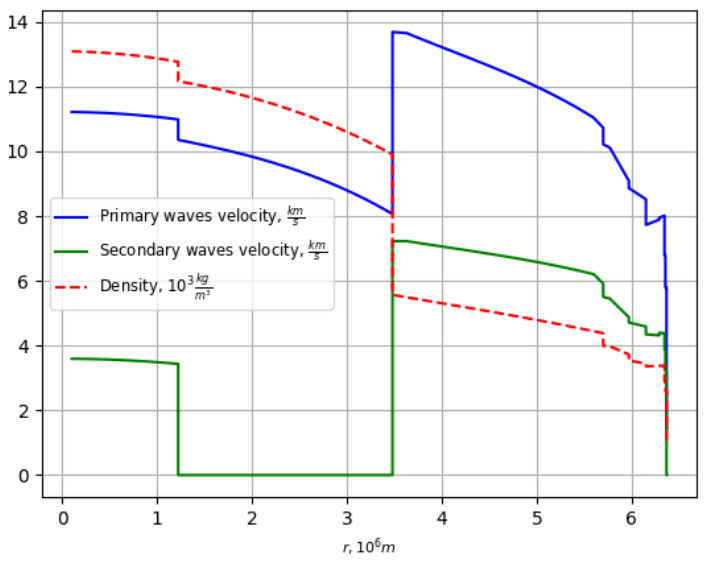
Those velocity–depth profiles (see Figure 1) are given by the travel-time distance curves for seismic waves and on periods of free oscillations [27,50,51]. Using a hydrostatic equilibrium equation, they provide pressure, density and elastic moduli profiles as functions of depth.

On the other hand, the seismic parameter (9) is related to the elastic properties of an isotropic material, that is, to the bulk modulus K (incompressibility)

$${\mathrm{\Phi }}_s={\displaystyle \frac{K}{\rho }}.$$

(10)

Applying the definition of the bulk modulus $K={\displaystyle \frac{dP}{d\ln \rho }}$, the seismic parameter can be written in terms of the material’s properties

$${\mathrm{\Phi }}_s={\displaystyle \frac{dP}{d\rho }},$$

(11)

such that it is clear now that it includes information on the equation of state. We can then use it in (7) to write

$${\displaystyle \frac{d\rho }{dr}}=-\rho {\mathrm{\Phi }}_s^{-1}{\displaystyle \frac{d\varphi }{dr}}.$$

(12)

Mass Equation (8) and moment of inertia

$$I={\displaystyle \frac{8}{3}}\pi {\int }_0^R{r}^4\rho \left(r\right)dr,$$

(13)

play a role of the constraints whose values are given by observations with a high accuracy [52,53].

4. Methodology

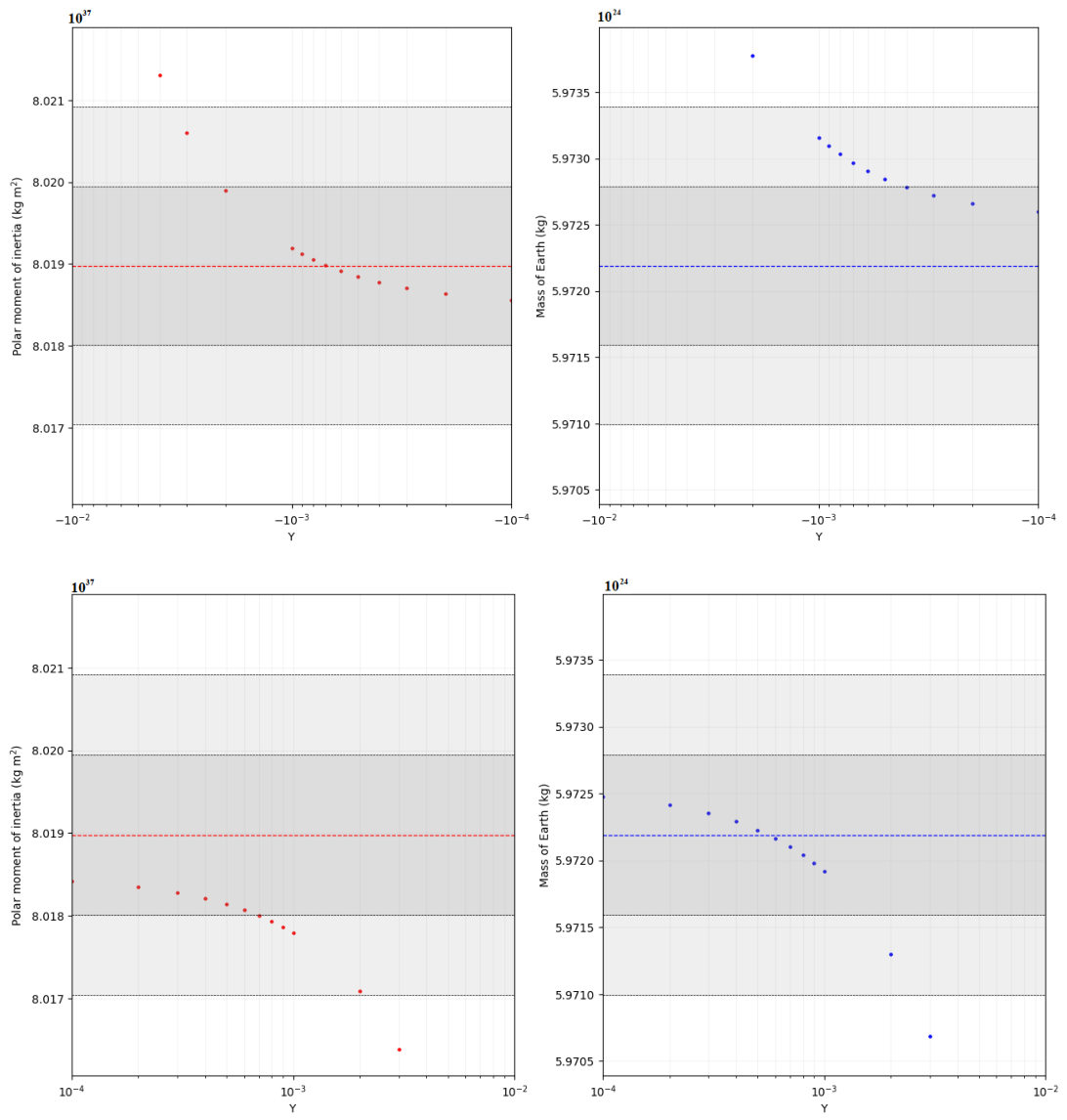
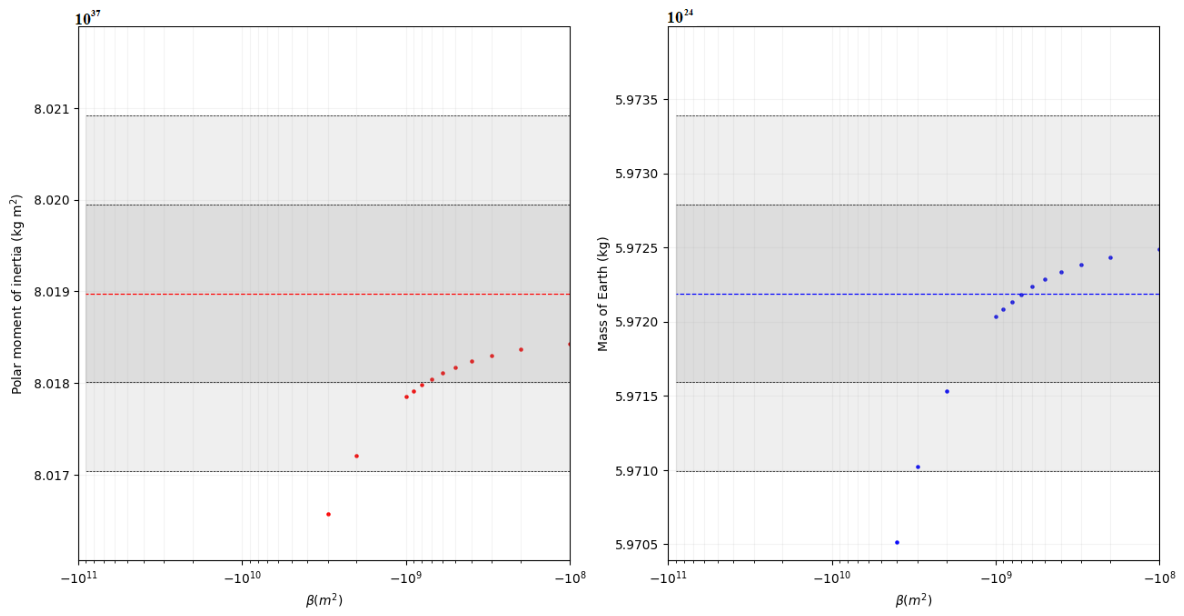
To go further, we base our calculations on the values of seismic wave velocities provided by [28], obtained within the framework of PREM. By assuming values for the free parameters of the PREM model, i.e., the density at the case of the mantle ${\rho }_m$, the density at the core ${\rho }_c$, and the density jump between the inner and the outer core $\Delta \rho$, we calculated the density profiles and obtained the total mass and polar moment of inertia. We aimed to obtain values that were consistent with those predicted by PREM, while accounting for the uncertainties arising from measurements. Our calculations were performed using a Python 3.7.3. script. We varied the values of $\beta$ and $\mathrm{{\rm Y}}$ and observed the effects on the calculations. We used a simplified model to assess the crucial parameters for more sophisticated analysis and to determine the order of magnitude of $\beta$ and $\mathrm{{\rm Y}}$ at which the effects of modified gravity are still in agreement with the observed constraints. Our results are shown in Figure 2 and Figure 3. The integration technique involved fitting a curve to the data points when finding the relation between the depth and the seismic parameter (in order to compute its derivative), and using the Euler method with initial conditions at corresponding boundaries; in other words, we integrated the system of two first-order differential equations outward, assuming the value of the central density and mass at the center, i.e., $M\left(0\right)=0$. We then computed the errors for a fixed set of parameters.

The Euler method, used in our integration scheme, is known to produce the local error of order $\mathcal{O}\left(h^2\right)$, where h is the step size. In our case, $h=\delta r$ is the spacing in the grid along the radial coordinate, over which we integrated the equations. The set of equations can then be written as

$$\begin{array}{cc}\hfill & \rho (r+\delta r)=\rho \left(r\right)+\delta rR(r,\rho \left(r\right),g\left(r\right))+{\displaystyle \frac{{\left(\delta r\right)}^2}{2}}{R}^{\prime }(\xi ,\rho \left(\xi \right),g\left(\xi \right)),\hfill \end{array}$$

(14)

$$\begin{array}{cc}\hfill & g(r+\delta r)=g\left(r\right)+\delta rG(r,\rho \left(r\right),g\left(r\right))+{\displaystyle \frac{{\left(\delta r\right)}^2}{2}}{G}^{\prime }(\xi ,\rho \left(\xi \right),g\left(\xi \right)),\hfill \end{array}$$

(15)

where ${\rho }^{\prime }\left(r\right)=R(r,\rho \left(r\right),g\left(r\right))$ and $g^{\prime }\left(r\right)=G(r,\rho \left(r\right),g\left(r\right))$, for some $\xi \in (r,r+\delta r)$. For the local error to be small, we choose $\delta r$ s.t. the quantities ${\displaystyle \frac{\delta r}{2}}{\displaystyle \frac{R^{\prime }}{R}}$ and ${\displaystyle \frac{\delta r}{2}}{\displaystyle \frac{G^{\prime }}{G}}$ are small. In order to estimate the error, we notice that one can make the following approximations (in the appropriate units): $g\sim 1$, $\rho \sim {10}^4$, ${\mathrm{\Phi }}_s\sim {10}^8$, ${\mathrm{\Phi }}_s^{\prime }\sim {10}^2$, ${\mathrm{\Phi }}_s^{″}\sim {10}^{-4}$; the estimates for the seismic parameter and its derivatives come from the analytic dependence ${\mathrm{\Phi }}_s\left(r\right)$ obtained by fitting a third degree polynomial to the data points. In the Palatini case, the result will not strongly depend on $\beta$ as long as $\left|\beta \right|<{10}^{12}$ m²; similar considerations are valid for the EiBI parameter. It was calculated that the ratios of order ${10}^{-3}$ of the quantities ${\displaystyle \frac{\delta r}{2}}{\displaystyle \frac{R^{\prime }}{R}}$ and ${\displaystyle \frac{\delta r}{2}}{\displaystyle \frac{G^{\prime }}{G}}$ are achieved for $\delta r=100$ m. The same integration step, guaranteeing a low local error, was taken when analyzing the DHOST theory.

It must be stressed that the central density’s value is not a result of solving differential equations, but rather an initial assumption. Additionally, we are not interested in modelling the outermost layers, since we expect the modifications of gravity to be weak there. For this reason, we assume Birch’s law to hold, and all the density values are taken directly from the PREM model. Then, we integrated (1), together with the mass relation (8), for different values of theories’ parameters. For the Ricci-based gravity, we performed calculations for $\beta \in [-{10}^{11}, {10}^{11}]{\mathrm{m}}^2$, while for the DHOST theories, the range of the theory’s parameter was $\mathrm{{\rm Y}}\in [-1, 1]$. The measure of goodness of the model with a particular choice of the corresponding parameter was the extent to which the calculated mass and polar moment of inertia agreed with the measured ones: $M_{\oplus }=(5.9722\pm 0.0006)\times {10}^{24}\mathrm{kg}$ [52] and $I_{\oplus }=(8.01736\pm 0.00097)\times {10}^{37}\mathrm{kg}{\mathrm{m}}^2$ [53].

Another important issue concerns the dependence of the seismic waves’ velocities on the local value of the density. The equation relating the values of the seismic waves’ velocities and the bulk modulus can be written as follows

$$K={\displaystyle \frac{dP}{dln\rho }}=\rho \left(v_p^2-{\displaystyle \frac{4}{3}}{v}_s^2\right)\Rightarrow {\displaystyle \frac{dP}{d\rho }}=v_p^2-{\displaystyle \frac{4}{3}}{v}_s^2.$$

(16)

Therefore, the velocities are related to the rate of change in pressure with density, and there is no direct, algebraic relation between them and the density. This result is strengthened by the analysis carried out by Kennet [54], in which the velocities of the seismic waves were also treated as measured. At the same time, the density distribution was altered to improve the fitting function predicted by the PREM model. What depends on the density distribution are the frequencies of the spheroidal and radial normal modes; using them for the calculated density profile would constitute an additional constraint on the theory. This issue is left as a topic of our future research.

5. Results and Discussion

Our study demonstrates that the following bounds can be placed on the considered parameters, ensuring that the deviations of Earth’s mass and polar moment of inertia do not exceed $2\sigma$. For Palatini $f\left(R\right)$ gravity, this value is approximately $-2\times {10}^9\lesssim \beta \lesssim {10}^9{\mathrm{m}}^2$. Similarly, for EiBI gravity, the value is around $-8\times {10}^9\lesssim ϵ\lesssim 4\times {10}^9{\mathrm{m}}^2$. In the case of the DHOST model, the constraint is $-{10}^{-3}\lesssim \mathrm{{\rm Y}}\lesssim {10}^{-3}$. It must be stressed that these results hold under the assumptions of the viability of the PREM model, exact knowledge of the density parameters, and clearly distinguished layers’ boundaries within the spherically symmetric model of the Earth. Taking into account possible uncertainties allows for a higher upper bound of the parameters; see the comments in the following part of the text.

Let us also present the constraints on these parameters coming from cosmology and astrophysics. First of all, let us notice that various analytical techniques, such as computing the PPN parameters, do not always provide values that allow one to differentiate between GR and a given theory in the vacuum; this is the case of the Palatini gravity [48] and the EiBI theory [55]. The presence of the dynamical scalar field in the DHOST theories could, in general, lead to alteration of the Solar System physics, but the model considered by us features the so-called Vainshtein mechanism, hiding the extra degree of freedom near massive bodies through non-linear effects [56].

Cosmological bounds placed on the Palatini parameter vary. In [57], the upper bound placed on $\beta$ is $\left|\beta \right|\lesssim {10}^{48}$ m² using the data coming from the CC+BAO dataset. Alternatively, the use of the Union2.1 dataset led to the value $\beta =-{0.092}_{-9.025}^{+8.840}\times {10}^{55}$ m² [58], although the model features also the term proportional to $1/R$, where R is the Palatini curvature; the $\beta$ parameter quantifies only the quadratic correction. The quadratic model itself was also analyzed in [59], where the value was constrained by $\left|\beta \right|\lesssim {10}^{43}$ m² utilizing data from the WMAP, 580 SNIa events. Moreover, the EiBI parameter was found to lie within $-6.1\times {10}^{15}\lesssim ϵ\lesssim 1.1\times {10}^{16}$ m² [60]. Lastly, the most stringent bound placed on the DHOST parameter $\mathrm{{\rm Y}}$ comes from helioseismology and was established to be $-{10}^{-3}\lesssim \mathrm{{\rm Y}}\lesssim 5\times {10}^{-4}$ [13], suggesting a better bound than the one obtained using our methodology. We expect, however, that the accuracy of our test will be improved when a more accurate, three-dimensional model of the planet is considered.

Considering PREM as a valid model for Earth, the uncertainties in the moment of inertia and mass provide bounds for the parameters. However, since PREM is not a perfect model, density parameters can differ from our assumptions. Current estimates placed on the density jump between the inner and the outer core vary from 300 kg m⁻³ to 900 kg m⁻³ [61], with the exact value depending on the position inside the Earth. Such a variation could not be taken into account by us for obvious reasons, but the ongoing investigation is aimed at creating a non-isotropic model of the Earth and calculating its density distribution. Moreover, other factors contributing to the uncertainties inherent to the model include the density at the center of the core, ranging from 12,760 kg m⁻³ to 13,090 kg m⁻³ [62]. Lastly, some alternative models to PREM have been considered; it was demonstrated that deviations in the density distribution by as much as 50 kg m⁻³ from the ones predicted by PREM can improve the density fitting function [54].

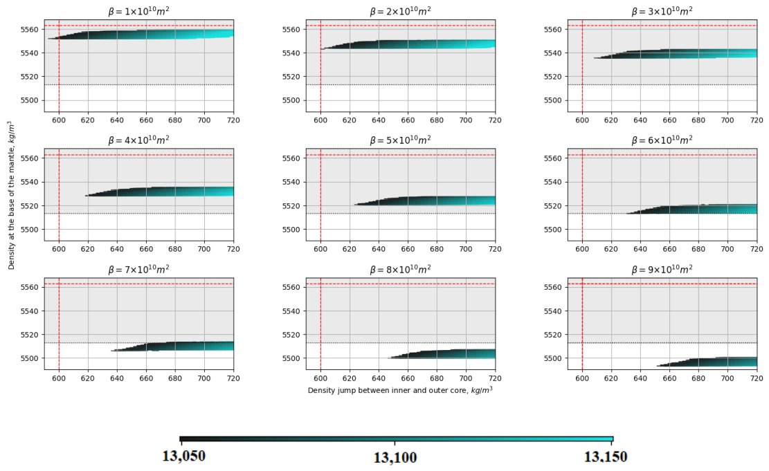
Notably, there exists a region for a given theory parameter where all three density parameters agree with experimental measurements (see our analysis in [9]). Among them, ${\rho }_m$ has a narrower range of variation compared to $\Delta \rho$ and ${\rho }_c$. As an example, for $\beta ={10}^9{\mathrm{m}}^2$, the deviations in ${\rho }_m$ required to maintain the same mass and polar moment of inertia, compared to the case when $\beta =0$ ($\mathrm{{\rm Y}}=0$), are very small, amounting to only $0.02\%$. However, the worst-case uncertainty in the PREM model, with deviations of about $50\mathrm{kg}{\mathrm{m}}^{-3}$, is $0.9\%$, while keeping $\Delta \rho$ and ${\rho }_c$ unchanged [9]. For such a deviation, the parameter increases by almost two orders of magnitude, as demonstrated in Figure 4. This shows that the impact of changing the theory parameter on ${\rho }_m$ is smaller than the uncertainty in the PREM model, which implies that the effect of the parameter on the results is relatively small compared to the uncertainties in the Earth model itself. Therefore, since the impact of the gravitational parameters on the possible range of ${\rho }_m$ is significant, reducing the uncertainty of ${\rho }_m$ by using a better Earth model will further improve our constraints on gravity models. Note that in this work we constrain models of gravity using the density parameters known from PREM, assuming that it is a viable model of Earth. On the other hand, the value of the model parameter is relatively uninfluenced by a simultaneous change in the density at the core and the density jump between the inner and the outer core, as an increase in the former can be compensated by an increase in the latter, leading to similar values of the total mass and the polar moment of inertia.

Our approach has limitations arising from assumptions and simplifications. However, to enhance this research, several potential extensions can be explored. The primary concern is assuming spherical symmetry, which fails to consider Earth’s actual shape and its sensitivity to rotation. To overcome this, we will focus on estimating the equatorial moment of inertia compared to the polar moment by incorporating travel time ellipticity corrections into the PREM model [31,63] in the near future.

Additionally, both PREM and our models are one-dimensional with spherical layers, which affect the moment of inertia and mass. Our future work should also consider the imperfections and density variations.

It is important to note that PREM does not consider seismic wave travel times sampling the boundaries of the outer and inner core, making it unsuitable to describe the deepest part of the planet. In order to take it into account, we will use the more accurate model AK135-F, which accounts for core wave complexity [31,63]. Moreover, equations of state can also be used to model core density and bulk moduli [64] rather than relying solely on seismic data.

Regarding Birch’s law, which describes the outer layers, it is an empirical law with experimentally obtained coefficients; it can be safely used in our case. However, if dealing with seismic data from Mars [65,66], the coefficients should be reevaluated due to different material compositions on each terrestrial planet.

An issue that has not been addressed in our paper is the impact of the density variation on the determination of the low eigenfrequency spheroidal modes. Any changes in the density distribution would influence the resultant eigenfrequencies, and that itself would constitute an effect that could be, in principle, measurable. In other words, computation of the low-order spherical modes could be used as a supplementary method of constraining the parameters of modified gravity theories. However, such a process would require calculating radial eigenfunctions under the assumption of the modified Poisson equation. In this paper, we focused only on the impact of the theory of gravity on the internal structure of the planet under the assumption that the seismic wave velocity profile is known and independent of the density distribution. Of course, our initial data were the velocities calculated using PREM and not the seismic waves’ travel times, based on which, one could compute the velocity profiles, but our methodology can be easily extended to the case of seismic waves’ velocity distribution in a way more independent of the model. The calculation of eigenfrequencies under the new density distribution is left as a future, complementary project that will bring more insight into the impact of modified gravity theories on the composition of Earth.

Another issue that requires addressing is the fact that, due to the specific form of the modification of the Newtonian limit in the Palatini and the EiBI theories, density discontinuities may give rise to potentially fatal singularities in the curvature [67]. This issue has been addressed in detail in Ref. [68], where it was demonstrated that, in the case of the Palatini $f\left(R\right)$ gravity, for the theory to be mathematically sound, the trace of the stress–energy tensor must be constant across matching hypersurfaces (similar argumentation can be made in the case of the EiBI theory). In our case, the trace of the stress–energy tensor is the density itself, so indeed, there might be some issues if our model corresponded to the actual structure of the planet. However, the core–mantle boundary (Bullen discontinuity) is not sharp, but rather features a very thin layer of varying rigidity and thickness [69]; the same can be said about the core–mantle boundary (Gutenberg discontinuity); more recent studies suggest that there might be a complex, compositionally layered transition zone between the core and the mantle, thus avoiding the sudden density jump [70].

6. Conclusions

Despite its current limitations, this study presents a valuable tool for constraining theories of gravity. With a relatively simple Earth model, we have successfully constrained the most popular Ricci-based gravities and scalar–tensor theories up to $2\sigma$. Notably, our approach considers matter and its properties, avoiding assumptions like vacuum, dust, or simple equations of state commonly made in other approaches. By encoding these properties into seismic wave data, we can better control uncertainties related to matter description and modified gravity effects, leading to more stringent bounds on theory parameters.

Moreover, continuous efforts to refine and enhance the method, as discussed earlier, are expected to yield even more robust constraints. The research is currently advancing in this promising direction. Despite the challenges encountered, the constraints obtained in this study hold substantial potential to significantly narrow down the range of plausible alternative gravity theories.

References

1. Huterer, D.; Turner, M.S. Prospects for probing the dark energy via supernova distance measurements. Phys. Rev. D 1999, 60, 081301. [Google Scholar] [CrossRef]
2. Saridakis, E.N.; Lazkoz, R.; Salzano, V.; Moniz, P.V.; Capozziello, S.; Jiménez, J.B.; De Laurentis, M.; Olmo, G.J. Modified Gravity and Cosmology: An Update by the CANTATA Network; Springer: Berlin/Heidelberg, Germany, 2021. [Google Scholar]
3. Langlois, D.; Noui, K. Hamiltonian analysis of higher derivative scalar-tensor theories. J. Cosmol. Astropart. Phys. 2016, 7, 016. [Google Scholar] [CrossRef]
4. Delhom, A.; Olmo, G.J.; Orazi, E. Ricci-Based Gravity theories and their impact on Maxwell and nonlinear electromagnetic models. J. High Energy Phys. 2019, 11, 149. [Google Scholar] [CrossRef]
5. Babichev, E.; Deffayet, C. An introduction to the Vainshtein mechanism. Class. Quant. Grav. 2013, 30, 184001. [Google Scholar] [CrossRef]
6. Koyama, K.; Sakstein, J. Astrophysical Probes of the Vainshtein Mechanism: Stars and Galaxies. Phys. Rev. D 2015, 91, 124066. [Google Scholar] [CrossRef]
7. Baker, T.; Psaltis, D.; Skordis, C. Linking Tests of Gravity On All Scales: From the Strong-Field Regime to Cosmology. Astroph. J. 2015, 802, 63. [Google Scholar] [CrossRef]
8. Kozak, A.; Wojnar, A. Metric-affine gravity effects on terrestrial exoplanet profiles. Phys. Rev. D 2021, 104, 084097. [Google Scholar] [CrossRef]
9. Kozak, A.; Wojnar, A. Planetary seismology as a test of modified gravity proposals. Phys. Rev. D 2023, 108, 044055. [Google Scholar] [CrossRef]
10. Kozak, A.; Pachoł, A.; Wojnar, A. Refining bounds for Snyder and GUP models through seismic wave analysis. Ann. Phys. 2025, 481, 170136. [Google Scholar] [CrossRef]
11. Bellinger, E.P.; Christensen-Dalsgaard, J. Asteroseismic Constraints on the Cosmic-time Variation of the Gravitational Constant from an Ancient Main-sequence Star. Astroph. J. Lett. 2019, 887, L1. [Google Scholar] [CrossRef]
12. Saltas, I.D.; Lopes, I. Obtaining Precision Constraints on Modified Gravity with Helioseismology. Phys. Rev. Lett. 2019, 123, 091103. [Google Scholar] [CrossRef] [PubMed]
13. Saltas, I.D.; Christensen-Dalsgaard, J. Searching for dark energy with the Sun. Astron. Astrophys. 2022, 667, A115. [Google Scholar] [CrossRef]
14. Abbott, B.P.; Abbott, R.; Abbott, T.; Acernese, F.; Ackley, K.; Adams, C.; Adams, T.; Addesso, P.; Adhikari, R.; Adya, V.B.; et al. GW170817: Observation of Gravitational Waves from a Binary Neutron Star Inspiral. Phys. Rev. Lett. 2017, 119, 161101. [Google Scholar] [CrossRef]
15. Patricelli, B.; Bernardini, M.G.; Mapelli, M.; D’Avanzo, P.; Santoliquido, F.; Cella, G.; Razzano, M.; Cuoco, E. Prospects for multimessenger detection of binary neutron star mergers in the fourth LIGO–Virgo–KAGRA observing run. Mon. Not. R. Astron. Soc. 2022, 513, 4159–4168. [Google Scholar] [CrossRef]
16. Baker, T.; Bellini, E.; Ferreira, P.G.; Lagos, M.; Noller, J.; Sawicki, I. Strong Constraints on Cosmological Gravity from GW170817 and GRB 170817A. Phys. Rev. Lett. 2017, 119, 251301. [Google Scholar] [CrossRef]
17. Ezquiaga, J.M.; Zumalacarregui, M. Dark Energy after GW170817: Dead ends and the road ahead. Phys. Rev. Lett. 2017, 119, 251304. [Google Scholar] [CrossRef]
18. Creminelli, P.; Vernizzi, F. Dark Energy after GW170817 and GRB170817A. Phys. Rev. Lett. 2017, 119, 251302. [Google Scholar] [CrossRef]
19. Sakstein, J.; Jain, B. Implications of the neutron star merger GW170817 for cosmological scalar-tensor theories. Phys. Rev. Lett. 2017, 119, 251303. [Google Scholar] [CrossRef]
20. Rezzolla, L.; Most, E.R.; Weih, L.R. Using gravitational-wave observations and quasi-universal relations to constrain the maximum mass of neutron stars. Astrophys. J. 2018, 852, L25. [Google Scholar] [CrossRef]
21. Fonseca, E.; Pennucci, T.T.; Ellis, J.A.; Stairs, I.H.; Nice, D.J.; Ransom, S.M.; Demorest, P.B.; Arzoumanian, Z.; Crowter, K.; Dolch, T.; et al. The NANOGrav Nine-year Data Set: Mass and Geometric Measurements of Binary Millisecond Pulsars. Astrophys. J. 2016, 832, 167. [Google Scholar] [CrossRef]
22. Cromartie, H.T.; Fonseca, E.; Ransom, S.M.; Demorest, P.B.; Arzoumanian, Z.; Blumer, H.; Brook, P.R.; DeCesar, M.E.; Dolch, T.; Ellis, J.A.; et al. Relativistic Shapiro delay measurements of an extremely massive millisecond pulsar. Nat. Astron. 2020, 4, 72–76. [Google Scholar] [CrossRef]
23. Olmo, G.J.; Rubiera-Garcia, D.; Wojnar, A. Stellar structure models in modified theories of gravity: Lessons and challenges. Phys. Rep. 2020, 876, 1–75. [Google Scholar] [CrossRef]
24. Kozak, A.; Soieva, K.; Wojnar, A. Cooling process of substellar objects in scalar-tensor gravity. Phys. Rev. D 2023, 108, 024016. [Google Scholar] [CrossRef]
25. Aguiar Gomes, D.; Wojnar, A. Early evolution of fully convective stars in scalar-tensor gravity. Eur. Phys. J. C 2023, 83, 492. [Google Scholar] [CrossRef]
26. Wojnar, A. Fermi gas and modified gravity. Phys. Rev. D 2023, 107, 044025. [Google Scholar] [CrossRef]
27. Poirier, J.-P. Introduction to the Physics of Earth’s Interior; Cambridge University Press: Cambridge, UK, 2000. [Google Scholar]
28. Dziewonski, A.M.; Anderson, D.L. Preliminary reference Earth model. Phys. Earth Plan. Int. 1981, 25, 297. [Google Scholar] [CrossRef]
29. Kustowski, B.; Ekström, G.; Dziewoński, A.M. Anisotropic shear-wave velocity structure of the Earth’s mantle: A global model. J. Geophys. Res. Solid Earth 2008, 113, B06306. [Google Scholar] [CrossRef]
30. Kennett, B.L.N.; Engdahl, E.R. Traveltimes for global earthquake location and phase identification. Geophys. J. Int. 1991, 105, 429. [Google Scholar] [CrossRef]
31. Kennett, B.L.N.; Engdahl, E.R.; Buland, R. Constraints on seismic velocities in the Earth from travel-times. Geophys. J. Int. 1995, 122, 108–124. [Google Scholar] [CrossRef]
32. Available online: https://ds.iris.edu/ds/products/emc-referencemodels (accessed on 22 July 2024).
33. Butler, R.; Tsuboi, S. Antipodal seismic reflections upon shear wave velocity structures within Earth’s inner core. Phys. Earth Planet. Int. 2021, 321, 106802. [Google Scholar] [CrossRef]
34. Frost, D.A.; Romanowicz, B. On the orientation of the fast and slow directions of anisotropy in the deep inner core. Phys. Earth Planet. Inter. 2019, 286, 101–110. [Google Scholar] [CrossRef]
35. Stephenson, J.; Tkalcic, H.; Sambridge, M.J. Evidence for the Innermost Inner Core: Robust Parameter Search for Radially Varying Anisotropy Using the Neighborhood Algorithm. Geophys. Res. Solid Earth 2021, 126, e2020JB020545. [Google Scholar] [CrossRef]
36. Pham, T.-S.; Tkalcic, H. Up-to-fivefold reverberating waves through the Earth’s center and distinctly anisotropic innermost inner core. Nat. Commun. 2023, 14, 754. [Google Scholar] [CrossRef]
37. Merkel, S.; Hok, S.; Bolme, C.; Rittman, D.; Ramos, K.J.; Morrow, B.; Lee, H.J.; Nagler, B.; Galtier, E.; Granados, E.; et al. Femtosecond Visualization of hcp-Iron Strength and Plasticity under Shock Compression. Phys. Rev. Lett. 2021, 127, 205501. [Google Scholar] [CrossRef] [PubMed]
38. Donini, A.; Palomares-Ruiz, S.; Salvado, J. Neutrino tomography of the Earth. Nat. Phys. 2019, 15, 37–40. [Google Scholar] [CrossRef]
39. Kozak, A.; Wojnar, A. Non-homogeneous exoplanets in metric-affine gravity. Int. J. Geom. Meth. Mod. Phys. 2022, 19, 2250157. [Google Scholar] [CrossRef]
40. Kozak, A.; Wojnar, A. Interiors of Terrestrial Planets in Metric-Affine Gravity. Universe 2021, 8, 3. [Google Scholar] [CrossRef]
41. Wojnar, A. Jupiter and jovian (exo)-planets in Palatini f( R ¯ ) gravity. Phys. Rev. D 2021, 104, 104058. [Google Scholar] [CrossRef]
42. Bills, B.G. Obliquity-oblateness feedback on Mars. J. Geophys. Res. Planets 1999, 104, 30773. [Google Scholar] [CrossRef]
43. Folkner, W.M.; Yoder, C.F.; Yuan, D.N.; Standish, E.M.; Preston, R.A. Interior Structure and Seasonal Mass Redistribution of Mars from Radio Tracking of Mars Pathfinder. Science 1997, 278, 1749–1752. [Google Scholar] [CrossRef] [PubMed]
44. Konopliv, A.S.; Sjogren, W.L. Publication 95-3; Jet Propulsion Laboratory, California Institute of Technology: La Cañada Flintridge, CA, USA, 1995. [Google Scholar]
45. Smith, D.E.; Lerch, F.J.; Nerem, R.S.; Zuber, M.T.; Patel, G.B.; Fricke, S.K.; Lemoine, F.G. An improved gravity model for Mars: Goddard Mars model 1. J. Geophys. Res. 1995, 98, 20871–20889. [Google Scholar] [CrossRef]
46. Folkner, W.M.; Kahn, R.D.; Preston, R.A.; Yoder, C.F.; Standish, E.M.; Williams, J.G.; Edwards, C.D.; Hellings, R.W.; Eubanks, T.M.; Bills, B.G. Mars dynamics from Earth-based tracking of the Mars Pathfinder lander. J. Geophys. Res. 1997, 102, 4057–4064. [Google Scholar] [CrossRef]
47. Williams, J.G. Contributions to the Earth’s obliquity rate, precession, and nutation. Astroph. J. 1994, 108, 711–724. [Google Scholar] [CrossRef]
48. Toniato, J.D.; Rodrigues, D.C.; Wojnar, A. Palatini f(R) gravity in the solar system: Post-Newtonian equations of motion and complete PPN parameters. Phys. Rev. D 2020, 101, 064050. [Google Scholar] [CrossRef]
49. Banados, M.; Ferreira, P.G. Eddington’s Theory of Gravity and Its Progeny. Phys. Rev. Lett. 2010, 105, 011101. [Google Scholar] [CrossRef] [PubMed]
50. Bolt, B.A. Inside Earth; W.H. Freeman & Co.: San Francisco, CA, USA, 1982. [Google Scholar]
51. Bullen, K.E.; Bolt, B.A. An Introduction to the Theory of Seismology; Cambridge University Press: Cambridge, UK, 1985. [Google Scholar]
52. Luzum, B.; Capitaine, N.; Fienga, A.; Folkner, W.; Fukushima, T.; Hilton, J.; Hohenkerk, C.; Krasinsky, G.; Petit, G.; Pitjeva, E.; et al. The IAU 2009 system of astronomical constants: The report of the IAU working group on numerical standards for Fundamental Astronomy. Celest. Mech. Dyn. Astron. 2011, 110, 293–304. [Google Scholar] [CrossRef]
53. Chen, W.; Ray, J.; Shen, W.B.; Huang, C.L. Consistent estimates of the dynamic figure parameters of the earth. J. Geod. 2015, 89, 179–188. [Google Scholar] [CrossRef]
54. Kennet, B.L.N. On the density distribution within the Earth. Geophys. J. Int. 1998, 132, 374–382. [Google Scholar] [CrossRef]
55. Pani, P.; Sotiriou, T.P. Surface singularities in Eddington-inspired Born-Infeld gravity. Phys. Rev. Lett. 2012, 109, 251102. [Google Scholar] [CrossRef]
56. Dima, A.; Vernizzi, F. Vainshtein Screening in Scalar-Tensor Theories before and after GW170817: Constraints on Theories beyond Horndeski. Phys. Rev. D 2018, 97, 101302. [Google Scholar] [CrossRef]
57. Gomes, D.A.; Briffa, R.; Kozak, A.; Levi Said, J.; Saal, M.; Wojnar, A. Cosmological constraints of Palatini f(R) gravity. J. Cosmol. Astropart. Phys. 2024, 2024, 011. [Google Scholar] [CrossRef]
58. Pinto, P.; Del Vecchio, L.; Fatibene, L.; Ferraris, M. Extended cosmology in Palatini f(R)-theories. J. Cosmol. Astropart. Phys. 2018, 2018, 044. [Google Scholar] [CrossRef]
59. Stachowski, A.; Szydlowski, M.; Borowiec, A. Starobinsky cosmological model in Palatini formalism. Eur. Phys. J. C 2017, 77, 406. [Google Scholar] [CrossRef]
60. Banerjee, P.; Garain, D.; Paul, S.; Shaikh, R.; Sarkar, T. A Stellar Constraint on Eddington-inspired Born–Infeld Gravity from Cataclysmic Variable Binaries. Astroph. J. 2022, 924, 20. [Google Scholar] [CrossRef]
61. Krasnoshchekov, D.N.; Ovtchinnikov, V.M. The Density Jump at the Inner Core Boundary in the Eastern and Western Hemispheres. Dokl. Earth Sci. 2018, 478, 219–223. [Google Scholar] [CrossRef]
62. Anderson, D.L. Theory of the Earth; Blackwell Scientific Publications: Oxford, UK, 1989. [Google Scholar]
63. Montagner, J.-P.; Kennett, B.L.N. How to reconcile body-wave and normal-mode reference Earth models. Geophys. J. Int. 1996, 125, 229–248. [Google Scholar] [CrossRef]
64. Irving, J.C.E.; Cottaar, S.; Lekic, V. Seismically determined elastic parameters for Earth’s outer core. Sci. Adv. 2018, 4, eaar2538. [Google Scholar] [CrossRef] [PubMed]
65. Horleston, A.C.; Clinton, J.F.; Ceylan, S.; Giardini, D.; Charalambous, C.; Irving, J.C.; Lognonné, P.; Stähler, S.C.; Zenhäusern, G.; Dahmen, N.L.; et al. The Far Side of Mars: Two Distant Marsquakes Detected by InSight. Seism. Rec. 2022, 2, 88–99. [Google Scholar] [CrossRef]
66. Irving, J.C.; Lekić, V.; Durán, C.; Xu, Z. First observations of core-transiting seismic phases on Mars. Proc. Natl. Acad. Sci. USA 2023, 120, e2217090120. [Google Scholar] [CrossRef] [PubMed]
67. Pani, P.; Sotiriou, T.P.; Vernieri, D. Gravity with Auxiliary Fields. Phys. Rev. D 2013, 88, 121502. [Google Scholar] [CrossRef]
68. Olmo, G.J.; Rubiera-Garcia, D. Junction conditions in Palatini f(R) gravity. Class. Quantum Grav. 2020, 37, 215002. [Google Scholar] [CrossRef]
69. Attanayake, J.; Thomas, C.; Cormier, V.F.; Miller, M.S.; Koper, K.D. Irregular Transition Layer Beneath the Earth’s Inner Core Boundary From Observations of Antipodal PKIKP and PKIIKP Waves. Geochem. Geophys. Geosyst. 2018, 19, 3607–3622. [Google Scholar] [CrossRef]
70. Russell, S.; Irving, J.C.E.; Myhill, R.; Cottaar, S. The emerging picture of a complex core-mantle boundary. Nat. Commun. 2024, 15, 4569. [Google Scholar] [CrossRef] [PubMed]
Figure 1. [color online] The density profile of the Earth according to the Preliminary Reference Earth Model (PREM) [9,28], which assumes Newtonian gravity. The velocity plots are derived from observational data without incorporating any gravitational theory. The primary waves refer to longitudinal waves, while the secondary waves are transverse waves.
Universe 12 00155 g001
Figure 2. [color online] Values of Earth’s mass and moment of inertia calculated for different values of the DHOST parameter Υ . The upper panel represents the results calculated for negative values of Υ , whereas the bottom one—for positive values. The figure on the left is plotted for the values of the moment of inertia; the figure on the right depicts the values of the mass of the planet. The dark gray stripe represents the 1-sigma region, and the light gray denotes the 2-sigma region. The dotted red line corresponds to the calculated value of Earth’s moment of inertia using the exact PREM parameters, whereas the dotted blue line corresponds to the calculated mass. The dots corresponding to different values of the theory parameter represent the value of the polar moment of inertia (red) and mass (blue) calculated for that value.
Universe 12 00155 g002
Figure 3. [color online] Values of Earth’s mass and moment of inertia calculated for different values of the Palatini parameter β . The figure on the left is plotted for the values of the moment of inertia; the figure on the right depicts the values of the mass of the planet. The dark gray stripe represents the 1-sigma region, and the light gray denotes the 2-sigma region. The figure for positive values of the β parameter can be found in [24]. The dotted red line corresponds to the calculated value of Earth’s moment of inertia using the exact PREM parameters, whereas the dotted blue line corresponds to the calculated mass. The dots corresponding to different values of the theory parameter represent the value of the polar moment of inertia (red) and mass (blue) calculated for that value.
Universe 12 00155 g003
Figure 4. [color online] 2 σ confidence regions of the theory parameters ( ρ c ,   ρ m ,   Δ ρ ) for different values of the β parameter. Lower values of the central density are related to darker shades of blue, while the larger values-to lighter; the range of the central density values, together with the corresponding colors, is shown in the color bar below the figures. The units are kg m−3. The red dashed lines represent the PREM values of the density jump and the density at the base of the mantle. The grey region corresponds to the maximum uncertainty in the determination of the density at the base of the mantle ρ m , which was assumed to be 50 kg m 3 (with respect to the PREM value).
Universe 12 00155 g004
Disclaimer/Publisher’s Note: The statements, opinions and data contained in all publications are solely those of the individual author(s) and contributor(s) and not of MDPI and/or the editor(s). MDPI and/or the editor(s) disclaim responsibility for any injury to people or property resulting from any ideas, methods, instructions or products referred to in the content.