Testing the Cosmological Principle in an Axisymmetric Metric from Ia SNe and CMB

Abstract

We investigate the possibility of testing the Cosmological Principle within a specific axisymmetric metric. Starting from the Einstein field equations, we derive a perturbed form of the Friedmann equation based on this metric and obtain a generalized form for matter density perturbations. By combining these, we establish the relationship between the scale factor a and the terms for matter density and dark energy over time. We then use the Union2.1 and PantheonPlus Type Ia supernovae datasets and CMB shift parameter R to constrain the perturbation parameters introduced in the model. This analysis allows us to assess whether matter perturbation could lead to observable inhomogeneity in cosmic expansion. Finally, we summarize the key parameters used in the calculation and discuss their physical significance. Our results indicate that within this axisymmetric metric, the contribution of matter perturbations to cosmic anisotropy and inhomogeneity is negligible, posing no challenge to the Cosmological Principle.

1. Introduction

The standard model of modern cosmology is based on the Cosmological Principle, which posits that the universe is homogeneous and isotropic on a large scale. This principle has been validated by the highly isotropic nature of cosmic microwave background radiation and forms the basis of the Friedmann equation. Nevertheless, whether cosmic expansion exhibits anisotropy and inhomogeneity remains an open question. Perturbations in cosmic expansion can manifest in two distinct forms: angular anisotropy and radial inhomogeneity. C. Bonvin et al. proposed the luminosity distance with perturbation [1], given a general formula for the luminosity distance, and recalculated the expression of the luminosity distance in perturbation FLRW space; meanwhile, they suggested a Doppler effect on the luminosity distance anisotropy, given the luminosity distance dipole formula [2]. However, H. A. Feldman et al. combined Ia Supernovae with the luminosity distance dipole formula to fit and found that the statistical direction of Bulk flow motion is not quite consistent in the solar system motion relative to the CMB ($l={263.85}^{\circ }\pm {0.1}^{\circ },b={48.25}^{\circ }\pm {0.04}^{\circ }$) [3,4]. Meanwhile, I. Antoniou employed a hemisphere comparison method and reported a maximum anisotropy ${\displaystyle \frac{\mathrm{\Delta }{\mathrm{\Omega }}_{0m}}{{\mathrm{\Omega }}_{0m}}}=0.43\pm 0.06$ [5,6].

On the other hand, R. Amanullah et al. fixed ${\mathrm{\Omega }}_m$ and calibrated Ia Supernovae using the SALT2 calibration method; they found when redshift is in range $0<z\le 1$, $M_B=-19.32,\alpha =0.12,\beta =2.47$, the calibration parameters values are more consistent in low redshift, and when the redshift is in range $z\ge 1$, $M_B=-19.45,\alpha =0.12,\beta =3.84$, the parameters are not quite consistent with low redshift [7]; there is some work on anisotropic investigations [8,9,10,11,12,13,14,15,16,17]. Furthermore the calculation value by $\mathrm{\Lambda }CDM$ is inconsistent with CMB redshift parameter R; this may be due to dark energy evolution over time that $\omega ={\displaystyle \frac{p}{\rho }}\ne -1$  [18,19,20], and it also may be caused by inhomogeneity in radial distance for cosmic expansion; K. Enqvist et al. discussed an inhomogeneous LTB metric, reconstructing the luminosity distance and Hubble rate changed with $z,r$  [21]. Meanwhile L. Campanelli et al. proposed an ellipsoidal metric to solve the CMB quadrupole anisotropy problem  [22,23]; T. Koivisto et al. also gave the anisotropy luminosity distance changed with the angle by the ellipsoidal metric [24,25].

These studies collectively suggest that the standard cosmological model may not fully account for the potential anisotropy or inhomogeneity in the universe, thereby motivating our investigation into the contribution of matter perturbations to cosmic anisotropy and inhomogeneity on large scales.

Before presenting our approach, it is important to clarify that the axisymmetric metric adopted in this work should not be identified with Bianchi-type models. While Bianchi cosmologies provide a well-established framework for exploring anisotropic yet spatially homogeneous universes, the metric introduced here is fundamentally inhomogeneous due to the presence of the radial- and angular-dependent function $b(r,\theta )$. The present analysis therefore probes a class of deviations distinct from those described by Bianchi classifications.

To address this issue, we adopt a specific axisymmetric metric and investigate whether potential matter density perturbations could lead to detectable signatures in cosmic expansion. We derive the relationship between the scale factor, the matter density term, and dark energy, and combine observational data to constrain the perturbation parameters. This approach allows us to test for the presence of such signals. In Section 2, we introduce a specific axisymmetric metric and impose the condition that the off-diagonal components of the energy–momentum tensor vanish. From this metric, the corresponding components of the Einstein tensor are computed. Under appropriate conditions, these geometric quantities reduce to the familiar form of the Friedmann equations. We ultimately obtain a luminosity distance formula that incorporates matter density perturbations. In Section 3, we use Union2.1 and PantheonPlus Ia supernova data [7,26,27,28] and the CMB shift parameter [29,30], combining calculated formulas to fit the perturbation parameters, and getting parameter statistical values and a confidence plane graph. In Section 4, we summarize the calculation results and analyze their significance.

2. The Matter Perturbation in the Axisymmetric Metric

2.1. Axisymmetric Metric

To explore the contribution of matter perturbations, we start with a certain axisymmetric perturbation metric in spherical coordinates, taking the general form:

$$d{s}^2=e^{2d(t,r,\theta )}{r}^2{sin}^2\theta d{\varphi }^2+e^{2a\left(t\right)}{e}^{2b(r,\theta )}(r^{2}d{\theta }^2+d{r}^2)-d{t}^2.$$

(1)

To simplify the calculation, we only focus on the radial and angular perturbations in the axisymmetric perturbation metric. Therefore, we impose the vanishing of the off-diagonal components of the Einstein tensor:

$$\begin{array}{c}{G}_{01}=0,\hfill \\ G_{02}=0,\hfill \\ G_{12}=0.\hfill \end{array}$$

(2)

These conditions serve as a simplifying constraint that forces $d(t,r,\theta )$ to be independent of r and $\theta$, thus reducing it to $a\left(t\right)$. Consequently, we obtain a specific axisymmetric perturbation metric:

$$d{s}^2=e^{2a\left(t\right)}{r}^2{sin}^2\theta d{\varphi }^2+e^{2a\left(t\right)}{e}^{2b(r,\theta )}(r^{2}d{\theta }^2+d{r}^2)-d{t}^2.$$

(3)

From the metric given in Equation (3), the non-zero components of the Einstein tensor are calculated as follows:

$$G_{00}=3{\left({\displaystyle \frac{\mathrm{d}}{\mathrm{d}t}}a\left(t\right)\right)}^2-e^{-2a\left(t\right)-2b(r,\theta )}{\displaystyle \frac{r^2\frac{{\partial }^2}{\partial r^2}b(r,\theta )+r\frac{\partial }{\partial r}b(r,\theta )+\frac{{\partial }^2}{\partial {\theta }^2}b(r,\theta )}{r^2}},$$

(4)

$$G_{11}=-e^{2a+2b}\left(2\ddot{a}+3{\dot{a}}^2\right)+{\displaystyle \frac{1}{r}}{\displaystyle \frac{\partial b}{\partial r}}-{\displaystyle \frac{cot\theta }{r^2}}{\displaystyle \frac{\partial b}{\partial \theta }},$$

(5)

$$G_{22}=-r^2{e}^{2a+2b}\left(2\ddot{a}+3{\dot{a}}^2\right)-r^2\left({\displaystyle \frac{1}{r}}{\displaystyle \frac{\partial b}{\partial r}}-{\displaystyle \frac{cot\theta }{r^2}}{\displaystyle \frac{\partial b}{\partial \theta }}\right),$$

(6)

$$\begin{array}{c}\hfill G_{33}=-r^2{sin}^2\theta e^{2a\left(t\right)}\left(2{\displaystyle \frac{{\mathrm{d}}^2}{\mathrm{d}{t}^2}}a\left(t\right)+3{\left({\displaystyle \frac{\mathrm{d}}{\mathrm{d}t}}a\left(t\right)\right)}^2\right)+r^2{sin}^2\theta e^{-2b(r,\theta )}{\displaystyle \frac{r^2\frac{{\partial }^2}{\partial r^2}b(r,\theta )+r\frac{\partial }{\partial r}b(r,\theta )+\frac{{\partial }^2}{\partial {\theta }^2}b(r,\theta )}{r^2}}\end{array}.$$

(7)

When the function $b(r,\theta )$ satisfies:

$${\displaystyle \frac{r^2\frac{{\partial }^2}{\partial r^2}b(r,\theta )+r\frac{\partial }{\partial r}b(r,\theta )+\frac{{\partial }^2}{\partial {\theta }^2}b(r,\theta )}{r^2}}=0,$$

(8)

$${\displaystyle \frac{1}{r}}{\displaystyle \frac{\partial b}{\partial r}}-{\displaystyle \frac{cot\theta }{r^2}}{\displaystyle \frac{\partial b}{\partial \theta }}=0.$$

(9)

Equations (4)–(7) degenerate into a Friedmann equation

$$G_{00}=3{\left({\displaystyle \frac{\mathrm{d}}{\mathrm{dt}}}a\left(t\right)\right)}^2,$$

(10)

$$G_{11}=G_{22}=G_{33}=3{\left({\displaystyle \frac{\mathrm{d}}{\mathrm{d}t}}a\left(t\right)\right)}^2+2\left({\displaystyle \frac{{\mathrm{d}}^2}{\mathrm{d}{t}^2}}a\left(t\right)\right).$$

(11)

2.2. The Matter Perturbation

To incorporate matter density perturbations, we rewrite Equation (4):

$$3{\left({\displaystyle \frac{\mathrm{d}}{\mathrm{dt}}}a\left(t\right)\right)}^2+{\displaystyle \frac{\left(\frac{{\partial }^2}{{\partial r^{\prime }}^2}{b}^{\prime }\left(r^{\prime },\theta \right)\right)r^2+\left(\frac{\partial }{\partial r^{\prime }}{b}^{\prime }\left(r^{\prime },\theta \right)\right)r+\left(\frac{{\partial }^2}{\partial {\theta }^2}{b}^{\prime }\left(r^{\prime },\theta \right)\right)}{{r^{\prime }}^2}}={\rho }_{\mathrm{\Lambda }}\left(t\right)+{\rho }_m(r^{\prime },\theta ).$$

(12)

Here we have introduced the radial coordinate $r^{\prime }={\mathrm{e}}^{a\left(t\right)+b\left(r,\theta \right)}r$, which absorbs the isotropic expansion and part of the perturbation.

$$\begin{array}{c}\hfill {\displaystyle \frac{\left(\frac{{\partial }^2}{\partial {r^{\prime }}^2}b\left(r^{\prime },\theta \right)\right)r^2+\left(\frac{\partial }{\partial r^{\prime }}b\left(r^{\prime },\theta \right)\right)r+\left(\frac{{\partial }^2}{\partial {\theta }^2}b\left(r^{\prime },\theta \right)\right)}{{r^{\prime }}^2}}=\\ \hfill {\rho }_{\mathrm{\Lambda }}\left(t\right)+{\rho }_m(r^{\prime },\theta )-3{\left({\displaystyle \frac{\mathrm{d}}{\mathrm{dt}}}a\left(t\right)\right)}^2.\end{array}$$

(13)

Equation (13) governs the spatial dependence of the perturbation $b(r^{\prime },\theta )$. Due to the axisymmetry of the problem and the separable structure of the differential operator, we seek solutions via the method of separation of variables. The angular part yields $cos\left(v\theta \right)$, while the radial part reduces to the Bessel equation. Expanding on the complete basis of Bessel functions, the general solution can be written as:

$$b(r^{\prime },\theta )={\displaystyle \sum _{v=0}^n}{\int }_0^{\infty }f\left(k\right)J_v\left(k{r}^{\prime }\right)cos\left(v\theta \right)dk,$$

(14)

where $J_v$ is the Bessel function of the first kind, and function $f\left(k\right)$ determines the amplitude of each mode and will be constrained by observational data.

To describe the matter density perturbation explicitly, we expand it in the same Bessel function as $b(r^{\prime },\theta )$:

$${\rho }_m(r^{\prime },\theta )={\rho }_m\left(t\right)+{\displaystyle \sum _{v=0}^n}{\int }_0^{\infty }f\left(k\right)J_v\left(k{r}^{\prime }\right)dkcos\left(v\theta \right).$$

(15)

Here the ${\rho }_m\left(t\right)$ represents the spatially averaged matter density.

The background expansion is governed by the Friedmann equation obtained from the spatial average of Equation (12):

$$3{\left({\displaystyle \frac{\mathrm{d}}{\mathrm{dt}}}a\left(t\right)\right)}^2={\rho }_m\left(t\right)+{\rho }_{\mathrm{\Lambda }}\left(t\right).$$

(16)

In Equation (3), the translational invariance in the time coordinate is:

$${\int }_{t_0}^{t_1}{\displaystyle \frac{dt}{{\mathrm{e}}^{2a\left(t\right)}}}={\int }_{t_0+\mathrm{\Delta }{t}_0}^{t_1+\mathrm{\Delta }{t}_1}{\displaystyle \frac{dt}{{\mathrm{e}}^{2a\left(t\right)}}}.$$

(17)

The relationship between redshift and time is also obtained by Equation (17):

$$1+z={\displaystyle \frac{e^{a\left(t_0\right)}}{e^{a\left(t_1\right)}}}.$$

(18)

Meanwhile we have the luminosity distance formula

$$d_l=(1+z){\int }_0^z{\displaystyle \frac{dz}{\dot{a}}}.$$

(19)

In the context of small perturbations and within the framework of the averaged energy–momentum tensor in cosmology, the conservation of matter energy–momentum is governed by the covariant divergence condition ${\nabla }_{\nu }{T}^{\mu \nu }=0$. Considering general relativity, the volume element of Equation (3) is $\sqrt{-g}{d}^{3}x=e^{3a\left(t\right)}{e}^{3b(r,\theta )}{r}^{2}sin\theta drd\theta d\varphi$. To study the evolution of the total mass enclosed within a large comoving spherical region of coordinate radius $r_w$, we integrate the time component of the conservation law over the spatial hypersurface. Under the assumption that the perturbation $b(r,\theta )$ is such that its effects on the overall volume average are negligible when the boundary is taken to infinity ($e^{a\left(t_0\right)}{r}_w\to \infty$), the volume element can be approximated by its background FLRW counterpart $R^{2}dR$ with $R=e^{a\left(t\right)}r$:

$$\begin{array}{c}\hfill {\int }_0^{e^{a\left(t\right)}{r}_w}({\rho }_m\left(t\right)+{\int }_0^{\infty }f\left(k\right)J_0\left(k{r}^{\prime }\right)dk)R^{2}dR=\\ \hfill {\int }_0^{e^{a\left(t_0\right)}{r}_w}({\rho }_m\left(t_0\right)+{\int }_0^{\infty }f\left(k\right)J_0\left(k{r}^{\prime }\right)dk)R^{2}dR.\end{array}$$

(20)

Using Equation (20), we obtain the evolution equation ${\rho }_m\left(t\right)$:

$$\begin{array}{c}\hfill {\rho }_m\left(t\right)={\rho }_m\left(t_0\right){\displaystyle \frac{e^{3a\left(t_0\right)}}{e^{3a\left(t\right)}}}+{\int }_0^{\infty }f\left(k\right)J_0\left(k{e}^{a\left(t_0\right)}{r}_w\right)dk{\displaystyle \frac{e^{3a\left(t_0\right)}}{e^{3a\left(t\right)}}}\\ \hfill -{\int }_0^{\infty }f\left(k\right)J_0\left(k{e}^{a\left(t\right)}{r}_w\right)dk\end{array}.$$

(21)

To proceed, we consider a specific simple form for $f\left(k\right)$, giving:

$$f\left(k\right)=N_m^{\prime }{k}^v,$$

(22)

where v is a free index characterizing the shape of the perturbation spectrum, and $N_m^{\prime }$ is an amplitude factor. The total amplitude of matter perturbation is

$$N_m=N_m^{\prime }{\int }_0^{\infty }{k}^v{J}_0\left(k{e}^{a\left(t_0\right)}{r}_w\right)dk.$$

(23)

Substituting Equations (18), (22) and (23) into Equation (21) yields the matter density:

$${\rho }_m\left(t\right)=({\rho }_m\left(t_0\right)+N_m)·{(1+z)}^3-N_m{(1+z)}^{v+1},$$

(24)

where ${\rho }_m\left(t\right)$ is not the average of matter density, but ${\rho }_m\left(t\right)\ne {\overline{\rho }}_m(r^{\prime },\theta )$.

Substituting Equation (24) into the luminosity distance formula, Equation (19), thereby gives the modified luminosity distance relation that accounts for matter perturbations:

$$d_l=(1+z)·{\displaystyle \frac{c}{H_0}}{\int }_0^z{\displaystyle \frac{dz}{\sqrt{({\mathrm{\Omega }}_m\left(t_0\right)+N_{{\mathrm{\Omega }}_m})·{(1+z)}^3-N_{{\mathrm{\Omega }}_m}{(1+z)}^{v+1}+1-{\mathrm{\Omega }}_m\left(t_0\right)}}}.$$

(25)

The parameter $N_{{\mathrm{\Omega }}_m}$ serves as a global factor for the perturbation amplitude: a value of zero corresponds to the unperturbed, homogeneous FLRW background. The index parameter v governs the spectral shape of the perturbation. The parameters ${\mathrm{\Omega }}_m$, $N_{{\mathrm{\Omega }}_m}$, and v are then constrained by fitting Equation (25) to observational data.

3. The Observation Data and Fitting Parameters

For our analysis, we utilize the Union2.1 Ia Supernovae obtained by R. Amanullah et al. [7], which employs the SALT2 calibration method and combines with $\mathrm{\Lambda }CDM$. We compute the ${\chi }^2$ statistic, defined as follows:

$${\chi }_{SNe}^2=\sum {\displaystyle \frac{{[\mu (\alpha ,\beta ,M_B)-\mu (z;{\mathrm{\Omega }}_m,N_{{\mathrm{\Omega }}_m},\nu )]}^2}{{\sigma }_{ext}^2+{\sigma }_{sys}^2+{\sigma }_{1c}^2}},$$

(26)

$${\sigma }_{1c}^2=V_{m_B}+{\alpha }^2{V}_{x_1}+{\beta }^2{V}_c+2\alpha V_{m_B,x_1}-2\beta V_{m_B,c}-2\alpha \beta V_{x_1,c},$$

(27)

where ${\sigma }_{1c}$ is the propagated error from the covariance matrix V. ${\sigma }_{ext}$ includes uncertainties due to host galaxy peculiar velocities of 300 km/s and uncertainties from Galactic extinction corrections and gravitational lensing. ${\sigma }_{sys}$ is the systematic error. The coefficients of the SALT2 calibration method $M_B,\alpha ,\beta$ take statistic values constrained by R. Amanullah et al. [7].

It is important to note that the form of the ${\chi }^2$ formula in Equation (26) arises because the non-systematic covariance matrix provided with Union2.1 is a diagonal matrix. In contrast, the systematic covariance matrix provided with the more recent PantheonPlus Ia Supernovae data [27,28] is non-diagonal. The PantheonPlus analysis represents the latest data in Ia SNe cosmology, providing improved calibration and a comprehensive covariance matrix. Consequently, when using PantheonPlus data, the ${\chi }^2$ formula must be generalized to a matrix form:

$${\chi }_{SNe}^2=\mathrm{\Delta }{\mu }^T·{\mathrm{C}}_{\mathrm{sys}}^{-1}·\mathrm{\Delta }\mu ,$$

(28)

$$\mathrm{\Delta }\mu ={\mu }_{obs}-\mu (z,{\mathrm{\Omega }}_m,N_{{\mathrm{\Omega }}_m},\nu ),$$

(29)

where the $\mathrm{C}$ denotes the full covariance matrix incorporating both statistical and systematic uncertainties.

We utilize the CMB shift parameter R  [29,30], which is given by  [29]:

$$R={\left({\mathrm{\Omega }}_m{H}_0^2\right)}^{1/2}{\int }_0^{z_{CMB}}{\displaystyle \frac{dz}{H\left(z\right)}}=1.70\pm 0.03.$$

(30)

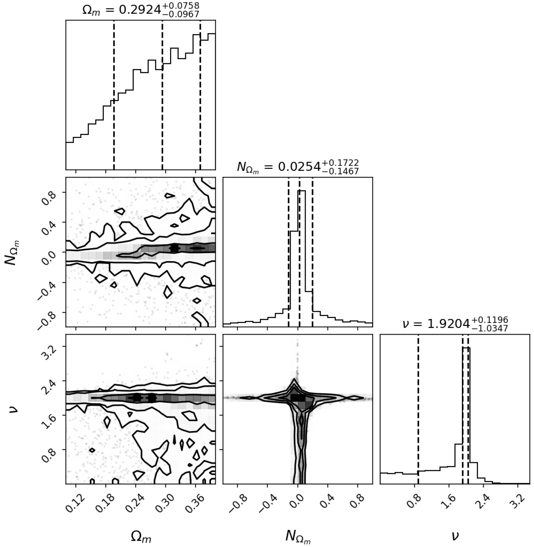
Based on the CMB shift parameter derived from theoretically homogeneous and isotropic CMB data, and applying it to our metric, we obtain the corresponding reference values for ${\mathrm{\Omega }}_m$, $N_{{\mathrm{\Omega }}_m}$, and $\nu$. These reference values, listed in

Table 1. The statistical values of the parameters ${\mathrm{\Omega }}_m$, $N_{{\mathrm{\Omega }}_m}$, $\nu$ from Union2.1 and PantheonPlus Ia SNe data; while Union2.1 set $H_0$ = 70 km/s/Mpc, PantheonPlus set $H_0$ = 73.5 km/s/Mpc. Among them, the numbers “¹” and “²” respectively denote the covariance matrices used with and without considering systematic effects. The CMB shift parameter provides a theoretical reference value derived under the assumption of homogeneity and isotropy, serving as a reference value to evaluate the degree of anisotropy in the supernova fits.

Observation Data	${\mathbf{\Omega }}_{\mathit{m}}$	${\mathit{N}}_{{\mathbf{\Omega }}_{\mathit{m}}}$	$\mathit{\nu }$
Union2.1 1	${0.28}_{-0.13}^{+0.14}$	${-0.03}_{-0.48}^{+0.45}$	${1.70}_{-1.04}^{+0.80}$
Union2.1 2	${0.28}_{-0.08}^{+0.09}$	${-0.02}_{-0.39}^{+0.39}$	${1.69}_{-1.07}^{+0.59}$
PantheonPlus 1	${0.31}_{-0.07}^{+0.05}$	${0.03}_{-0.32}^{+0.36}$	${1.75}_{-1.21}^{+0.50}$
CMB	${0.29}_{-0.10}^{+0.08}$	${0.02}_{-0.14}^{+0.17}$	${1.92}_{-1.03}^{+0.12}$

and Figure 1, serve as benchmarks: comparing the supernova results with these reference values allows us to quantify the deviation of Ia SNe data from those of the homogeneous and isotropic CMB data within the axisymmetric matter perturbation model. This enables a discussion of the contribution of matter perturbation parameters to cosmic inhomogeneity and anisotropy.

We also utilize the Union2.1 Ia SNe data, which include systematic errors. We perform parameter fitting using the emcee [31] to constrain the parameters in Equations (25), (26) and (28), thereby obtaining the statistical values presented in Table 1, and the confidence plane graph in Figure 1, Figure 2, Figure 3 and Figure A1.

For the supernova analysis, we adopt uniform priors on the parameters: ${\mathrm{\Omega }}_m\in [0,1]$, $N_{{\mathrm{\Omega }}_m}\in [-1,1]$, and $\nu \in [0,5]$. The likelihood is constructed as $\mathcal{L}\propto exp(-{\chi }^2/2)$ with ${\chi }^2=\mathrm{\Delta }{\mu }^T{C}^{-1}\mathrm{\Delta }\mu ,$ where $\mathrm{\Delta }\mu$ is the residual between the observed and theoretical distance modulus, and C is the covariance matrix.

For the CMB analysis, the parameter ranges are appropriately adjusted, with uniform priors taken as ${\mathrm{\Omega }}_m\in [0.1,0.4]$, $N_{{\mathrm{\Omega }}_m}\in [-1,1]$, and $\nu \in [0,5]$. The corresponding likelihood is constructed as $\mathcal{L}\propto exp(-{\chi }^2/2)$ with ${\chi }^2={[R({\mathrm{\Omega }}_m,N_{{\mathrm{\Omega }}_m},\nu )-1.70]}^2,$ where R is computed by numerical integration of Equation (30).

For all MCMC runs, we use the emcee ensemble sampler with 32 walkers, run for 3000 steps, discard the first 500 steps as burn-in, and thin the chain by a factor of 15 to reduce autocorrelation. Convergence is assessed by visually inspecting the chain traces to ensure they are well constrained.

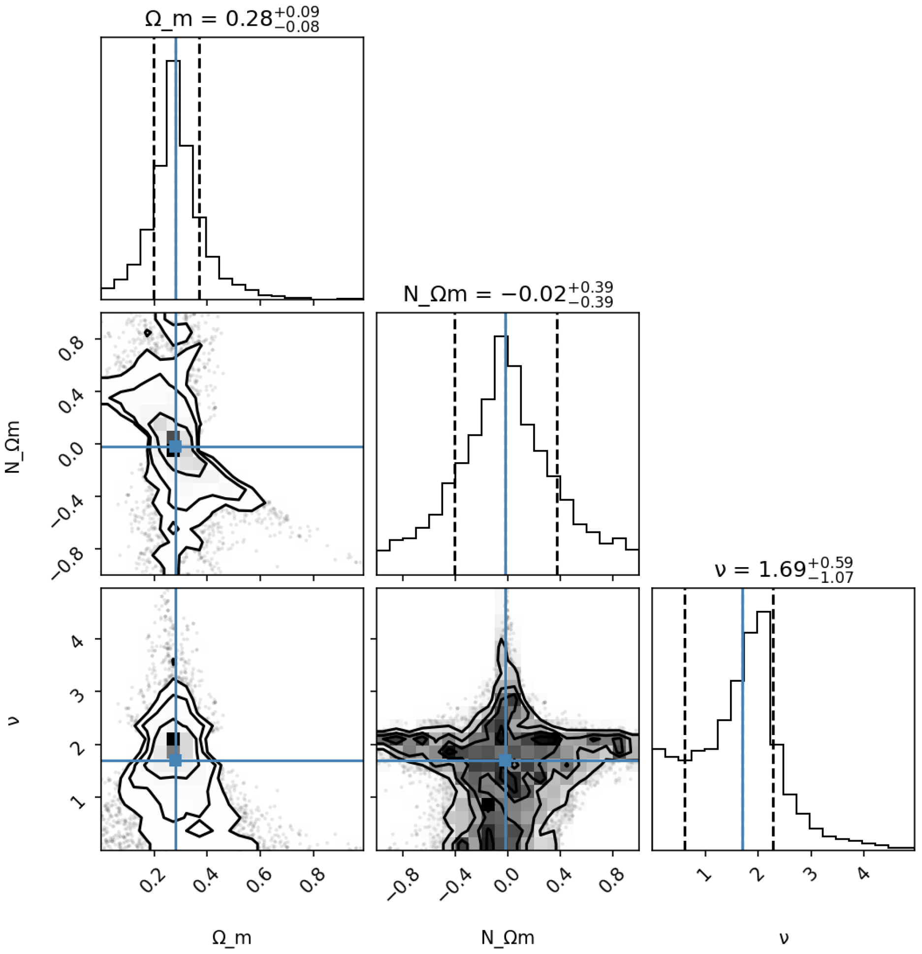
Figure 2 shows the best-fit values and confidence contours for the parameter pairs $({\mathrm{\Omega }}_m,N_{{\mathrm{\Omega }}_m})$, $({\mathrm{\Omega }}_m,\nu )$, and $(N_{{\mathrm{\Omega }}_m},\nu )$, obtained from the Union2.1 dataset (using the non-systematic covariance matrix) in combination with Equations (25) and (26). The contours reveal a mild anti-correlation between ${\mathrm{\Omega }}_m$ and $N_{{\mathrm{\Omega }}_m}$. The confidence region for $\nu$ is notably broad along the $N_{{\mathrm{\Omega }}_m}$ direction, indicating that the current data provide only a weak constraint on the geometrical morphology index $\nu$. Crucially, the posterior for $N_{{\mathrm{\Omega }}_m}$ is consistent with zero within its $1\sigma$ and $2\sigma$ confidence intervals, showing no statistically significant detection of a matter density perturbation amplitude within this model and dataset.

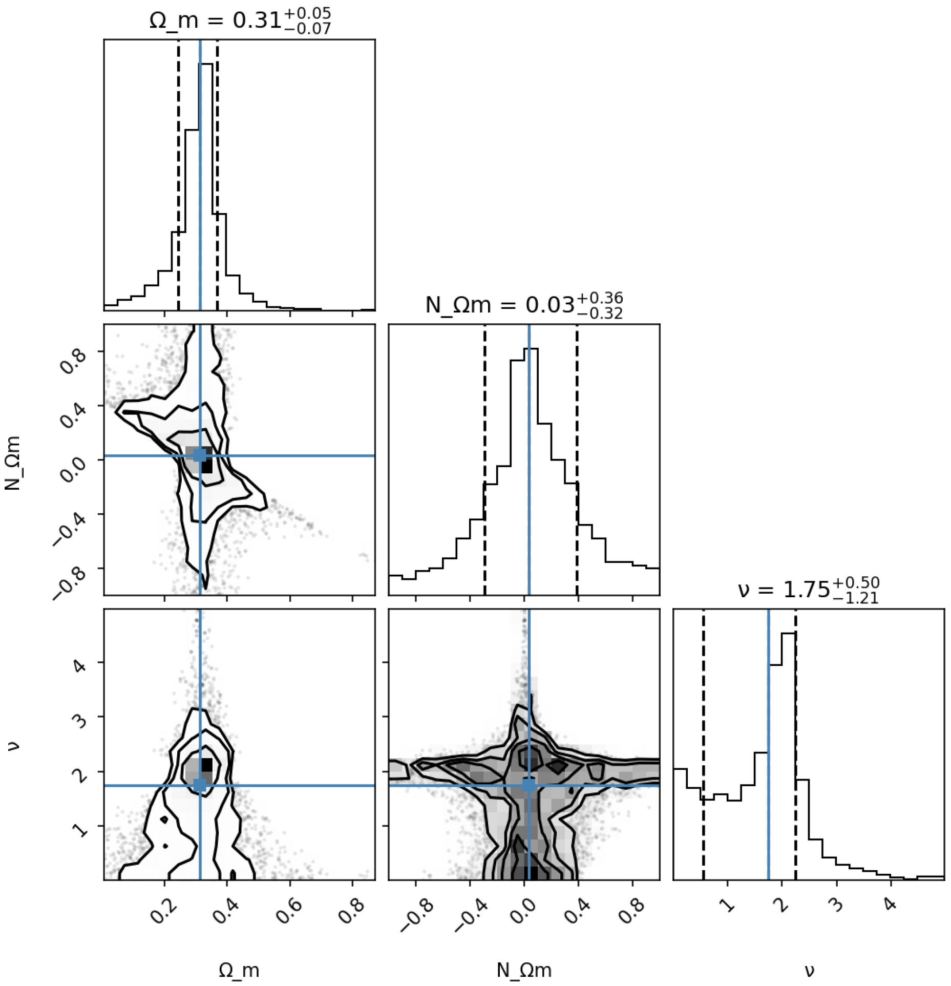
Figure 3 presents the equivalent constraints derived from the PantheonPlus dataset combined with Equations (25) and (29). The overall structure of the confidence contours is similar to that in Figure 2. The constraint on $N_{{\mathrm{\Omega }}_m}$ remains consistent with zero. The PantheonPlus data, benefiting from a more comprehensive treatment of systematic uncertainties via its full covariance matrix, generally yield tighter constraints, particularly on ${\mathrm{\Omega }}_m$. However, the constraint on the index $\nu$ remains weak, with large uncertainties persisting.

Figure 1 displays the parameter constraints obtained from the CMB shift parameter R using Equation (29). It should be noted that the CMB provides only a single integrated distance point (the R parameter), while the model contains multiple free parameters (${\mathrm{\Omega }}_m,N_{{\mathrm{\Omega }}_m},\nu$). In an unrestricted fit, a likelihood extreme value appears around ${\mathrm{\Omega }}_m\approx 0.6$, which is inconsistent with the widely accepted cosmological value of matter density (${\mathrm{\Omega }}_m\sim 0.3$) and constitutes an unphysical solution. To exclude this unrealistic region, we imposed a loose prior on ${\mathrm{\Omega }}_m$ based on current consensus (${\mathrm{\Omega }}_m\in [0.1,0.4]$) to ensure the fit remains within a physically plausible range. This restriction applies only to ${\mathrm{\Omega }}_m$; no additional priors were applied to $N_{{\mathrm{\Omega }}_m}$ or $\nu$. Thus, the confidence contours shown in the figure truthfully reflect the allowable ranges of these two parameters under the current model and data.

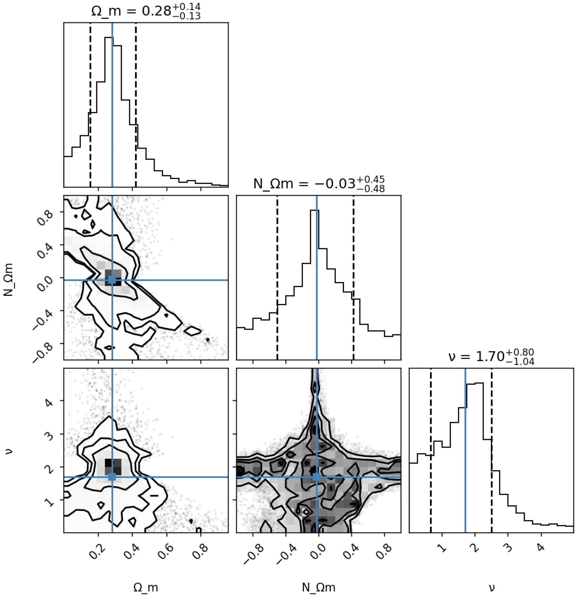
Figure A1 in the appendix shows the constraints from the Union2.1 data (systematic covariance matrix) using Equations (25) and (28), serving as a consistency check. The resulting contours are virtually identical to those in Figure 2, confirming the robustness of the analysis against the specific statistical treatment of this dataset.

4. Analysis and Summary of Parameter Values

This study conducts a quantitative test of the homogeneity of large-scale cosmic expansion within the framework of an axisymmetric metric, incorporating a parameterized matter density perturbation and utilizing the PantheonPlus and Union2.1 Type Ia supernova, alongside a CMB shift parameter-derived theoretical reference baseline.

The analysis finds no statistically significant signal for matter density perturbations: the PantheonPlus dataset yields $N_{{\mathrm{\Omega }}_m}={0.03}_{-0.32}^{+0.36}$, the Union2.1 gives $N_{{\mathrm{\Omega }}_m}={-0.02}_{-0.39}^{+0.39}$, and the reference value obtained from the CMB shift parameter gives $N_{{\mathrm{\Omega }}_m}={0.025}_{-0.14}^{+0.17}$, with their $1\sigma$ confidence intervals robustly encompassing zero. The potential influence of matter density perturbations on cosmic expansion anisotropy and inhomogeneity is primarily probed through the deviation of the index $\nu$ from a value of two. When using Ia SNe, the fitting value ${\nu }_{union2.1}={1.69}_{-1.07}^{+0.59}$, and ${\nu }_{pantheonplus}={1.75}_{-1.21}^{+0.50}$. Although the best-fit values of the anisotropy index $\nu$ vary across different datasets, their uncertainties are generally large, both of which are compatible with the theoretical reference value ${\nu }_{cmb}={1.92}_{-1.03}^{+0.12}$ within their large uncertainties.

Notably, the PantheonPlus dataset is the largest and most recent compilation of Type Ia supernovae. It can be clearly seen from the figure that compared to the Union2.1 dataset, the constraints of PantheonPlus are more stringent, and the deviation between the results and the reference values is smaller. This indicates that with the improvement of observation accuracy, the deviation between supernova data results and homogeneous and isotropic CMB data results decreases and approaches zero, reflecting that the contribution of matter perturbation to the anisotropy and inhomogeneity of the universe under the axisymmetric metric is small and does not pose a challenge to the Cosmological Principle.

In conclusion, within the axisymmetric perturbation framework, the analysis of Type Ia supernova data indicates that the contribution of matter perturbations to the universe’s inhomogeneity and anisotropy is extremely small, and the observational results align well with homogeneous and anisotropic CMB results.

These results establish quantitative upper limits on the amplitude of such perturbations, further reinforcing the validity of the Cosmological Principle. Future missions, such as the Roman Space Telescope, Euclid, and the Square Kilometre Array (SKA), will deliver orders-of-magnitude increases in supernova, galaxy, and mapping surveys, enabling definitive tests of fundamental cosmic symmetries.

References

1. Bonvin, C.; Durrer, R.; Gasparini, M.A. Fluctuations of the Luminosity Distance. Phys. Rev. D 2005, 73, 023523. [Google Scholar] [CrossRef]
2. Bonvin, C.; Durrer, R.; Kunz, M. The Dipole of the Luminosity Distance: A Direct Measure of H(z). Phys. Rev. Lett. 2006, 96, 191302. [Google Scholar] [CrossRef]
3. Colin, J.; Mohayaee, R.; Sarkar, S.; Shafieloo, A. Probing the Anisotropic Local Universe and Beyond with SNe Ia Data. Mon. Not. R. Astron. Soc. 2011, 414, 264–271. [Google Scholar] [CrossRef]
4. Wang, J.S.; Wang, F.Y. Probing the Anisotropic Expansion from Supernovae and GRBs in a Model-Independent Way. Mon. Not. R. Astron. Soc. 2014, 443, 1680–1687. [Google Scholar] [CrossRef]
5. Antoniou, I.; Perivolaropoulos, L. Searching for a Cosmological Preferred Axis: Union2 Data Analysis and Comparison with Other Probes. J. Cosmol. Astropart. Phys. 2010, 2010, 012. [Google Scholar] [CrossRef]
6. Yang, X.; Wang, F.Y.; Chu, Z. Searching for a Preferred Direction with Union2.1 Data. Mon. Not. R. Astron. Soc. 2013, 437, 1840–1846. [Google Scholar] [CrossRef]
7. Amanullah, R.; Lidman, C.; Rubin, D.; Aldering, G.; Astier, P.; Barbary, K.; Burns, M.S.; Conley, A.; Dawson, K.S.; Deustua, S.E.; et al. Spectra and Light Curves of Six Type Ia Supernovae at 0.511 < z < 1.12 and the Union2 Compilation. Astrophys. J. 2010, 716, 712–738. [Google Scholar] [CrossRef]
8. Colin, J.; Mohayaee, R.; Rameez, M.; Sarkar, S. Evidence for Anisotropy of Cosmic Acceleration. Astron. Astrophys. 2019, 631, L13. [Google Scholar] [CrossRef]
9. Javanmardi, B.; Porciani, C.; Kroupa, P.; Pflamm-Altenburg, J. Probing the Isotropy of Cosmic Acceleration Traced by Type Ia Supernovae. Astrophys. J. 2015, 810, 47. [Google Scholar] [CrossRef]
10. Hu, J.P.; Wang, Y.Y.; Hu, J.; Wang, F.Y. Testing the Cosmological Principle with the Pantheon+ Sample and the Region-Fitting Method. arXiv 2023, arXiv:2310.11727. [Google Scholar] [CrossRef]
11. Saadeh, D.; Feeney, S.M.; Pontzen, A.; Peiris, H.V.; McEwen, J.D. How Isotropic is the Universe? Phys. Rev. Lett. 2016, 117, 131302. [Google Scholar] [CrossRef]
12. Wang, Y.Y.; Wang, F.Y. Testing the Isotropy of the Universe with Type Ia Supernovae in a Model-Independent Way. Mon. Not. R. Astron. Soc. 2017, 474, 3516–3522. [Google Scholar] [CrossRef]
13. Rameez, M.; Mohayaee, R.; Sarkar, S.; Colin, J. The Dipole Anisotropy of AllWISE Galaxies. Mon. Not. R. Astron. Soc. 2018, 477, 1772–1781. [Google Scholar] [CrossRef]
14. Eriksen, H.K.; Hansen, F.K.; Banday, A.J.; Górski, K.M.; Lilje, P.B. Asymmetries in the Cosmic Microwave Background Anisotropy Field. Astrophys. J. 2004, 605, 14–20. [Google Scholar] [CrossRef]
15. Nadolny, T.; Durrer, R.; Kunz, M.; Padmanabhan, H. A New Way to Test the Cosmological Principle: Measuring Our Peculiar Velocity and the Large-Scale Anisotropy Independently. J. Cosmol. Astropart. Phys. 2021, 2021, 9. [Google Scholar] [CrossRef]
16. Hansen, F.K.; Banday, A.J.; Górski, K.M.; Eriksen, H.K.; Lilje, P.B. Power Asymmetry in Cosmic Microwave Background Fluctuations from Full Sky to Sub-Degree Scales: Is the Universe Isotropic? Astrophys. J. 2009, 704, 1448–1458. [Google Scholar] [CrossRef]
17. Franco, C.; Avila, F.; Bernui, A. Probing Cosmic Isotropy in the Local Universe. Mon. Not. R. Astron. Soc. 2023, 527, 7400–7413. [Google Scholar] [CrossRef]
18. Chevallier, M.; Polarski, D. Accelerating Universes with Scaling Dark Matter. Int. J. Mod. Phys. D 2001, 10, 213–223. [Google Scholar] [CrossRef]
19. Linder, E.V. Exploring the Expansion History of the Universe. Phys. Rev. Lett. 2003, 90, 091301. [Google Scholar] [CrossRef] [PubMed]
20. Capozziello, S.; Lazkoz, R.; Salzano, V. Comprehensive Cosmographic Analysis by Markov Chain Method. Phys. Rev. D 2011, 84, 124061. [Google Scholar] [CrossRef]
21. Enqvist, K. Lemaitre-Tolman-Bondi Model and Accelerating Expansion. Gen. Relativ. Gravit. 2007, 40, 451–466. [Google Scholar] [CrossRef]
22. Campanelli, L.; Cea, P.; Tedesco, L. Ellipsoidal Universe Can Solve the Cosmic Microwave Background Quadrupole Problem. Phys. Rev. Lett. 2006, 97, 131302. [Google Scholar] [CrossRef] [PubMed]
23. Koivisto, T.; Mota, D.F. Accelerating Cosmologies with an Anisotropic Equation of State. Astrophys. J. 2008, 679, 1–5. [Google Scholar] [CrossRef]
24. Koivisto, T.; Mota, D.F. Anisotropic Dark Energy: Dynamics of Background and Perturbations. J. Cosmol. Astropart. Phys. 2008, 2008, 018. [Google Scholar] [CrossRef]
25. Campanelli, L.; Cea, P.; Fogli, G.L.; Marrone, A. Testing the Isotropy of the Universe with Type Ia Supernovae. Phys. Rev. D 2011, 83, 103503. [Google Scholar] [CrossRef]
26. Suzuki, N.; Rubin, D.; Lidman, C.; Aldering, G.; Amanullah, R.; Barbary, K.; Barrientos, L.F.; Botyanszki, J.; Brodwin, M.; Connolly, N.; et al. The Hubble Space Telescope Cluster Supernova Survey: V. Improving the Dark Energy Constraints Above z > 1 and Building an Early-Type-Hosted Supernova Sample. Astrophys. J. 2011, 746, 85. [Google Scholar] [CrossRef]
27. Brout, D.; Scolnic, D.; Popovic, B.; Riess, A.G.; Carr, A.; Zuntz, J.; Kessler, R.; Davis, T.M.; Hinton, S.; Jones, D.; et al. The Pantheon+ Analysis: Cosmological Constraints. Astrophys. J. 2022, 938, 110. [Google Scholar] [CrossRef]
28. Riess, A.G.; Yuan, W.; Macri, L.M.; Scolnic, D.; Brout, D.; Casertano, S.; Jones, D.O.; Murakami, Y.; Anand, G.S.; Breuval, L.; et al. A Comprehensive Measurement of the Local Value of the Hubble Constant with 1 km s−1 Mpc−1 Uncertainty from the Hubble Space Telescope and the SH0ES Team. Astrophys. J. Lett. 2022, 934, L7. [Google Scholar] [CrossRef]
29. Nesseris, S.; Perivolaropoulos, L. Crossing the Phantom Divide: Theoretical Implications and Observational Status. J. Cosmol. Astropart. Phys. 2007, 2007, 018. [Google Scholar] [CrossRef]
30. Wang, Y.; Tegmark, M. New Dark Energy Constraints from Supernovae, Microwave Background, and Galaxy Clustering. Phys. Rev. Lett. 2004, 92, 241302. [Google Scholar] [CrossRef] [PubMed]
31. Foreman-Mackey, D.; Hogg, D.W.; Lang, D.; Goodman, J. emcee: The MCMC Hammer. Publ. Astron. Soc. Pac. 2013, 125, 306–312. [Google Scholar] [CrossRef]
Figure 1. The best fitting value and the confidence plane of the parameters ( Ω m , N Ω m ), ( Ω m , ν ), ( N Ω m , ν ) from CMB data combined with Equation (29); the density parameters Ω m are subject to strict constraints and are restricted to the values of 0.1 and 0.4. The dash line mark the 1 σ range, the colors shadow indicate the density of scattered points.
Universe 12 00156 g001
Figure 2. The best fitting value and the confidence plane of the parameters ( Ω m , N Ω m ), ( Ω m , ν ), ( N Ω m , ν ) from Union2.1 data (non-systematic covariance matrix) combined with Equations (24) and (25). The shape of the covariance matrix is 580 × 580, and the graphic shape is relatively divergent (compare with Figure 3). The dash line mark the 1 σ range, the colors shadow indicate the density of scattered points and the blue line denotes the central estimate.
Universe 12 00156 g002
Figure 3. The best fitting value and the confidence plane of the parameters ( Ω m , N Ω m ), ( Ω m , ν ), ( N Ω m , ν ) from PantheonPlus data combined with Equations (24) and (27). The shape of the covariance matrix is 1701 × 1701, and the graphic shape is relatively convergent (compare with Figure 2). The dash line mark the 1 σ range, the colors shadow indicate the density of scattered points and the blue line denotes the central estimate.
Universe 12 00156 g003