Constraining the Quantum Gravity Energy Scale via Gamma-Ray Burst Spectral Lag Data

Abstract

Lorentz invariance violation (LIV) can alter the group velocity of photons by modifying their dispersion relation, manifesting as differences in the arrival times of photons with different energies. This effect can accumulate over long propagation distances, making gamma-ray bursts (GRBs) a key tool for probing Lorentz invariance violation. By analyzing spectral lag data from 360 measurements across 90 GRBs using Markov Chain Monte Carlo (MCMC) sampling, and under the assumption that all GRBs share a common intrinsic time delay function, we report a maximum a posteriori value of the energy scale of quantum gravity at linear order $E_{QG}=8.96\times {10}^{14}$ GeV, though the data are also compatible with Lorentz invariance ($E_{\mathrm{QG}}=\infty$) to within $2.8\sigma$. Furthermore, we are $95\%$ confident that $E_{QG}\ge 6.67\times {10}^{14}$ GeV.

1. Introduction

Quantum gravity theories such as loop quantum gravity and string theory often predict a breakdown of Lorentz invariance at extremely high energy scales comparable to the Planck scale [1,2,3,4,5,6,7]. One generic prediction of Lorentz invariance violation is an energy-dependent vacuum dispersion of photons [1,8]. In LIV scenarios, the group velocity of a photon in a vacuum would vary slightly with its energy, contrary to exact Lorentz invariance which demands a constant c. Although any LIV-induced deviation from c is minuscule at laboratory-accessible energies, over cosmological propagation distances these tiny differences can accumulate into measurable time-of-flight differences [9,10,11,12,13,14,15,16,17].

GRBs serve as ideal cosmic probes for testing such effects. GRBs are brief flashes of intense $\gamma$ rays from the distant universe (redshifts $z=0.34$–$5.6$ in our sample), associated with catastrophic events such as stellar collapses or compact object mergers. They emit across a broad energy range (from radio to GeV and sometimes even TeV energies) and are detected at cosmological distances, making them sensitive probes of energy-dependent propagation delays. Crucially, if high-energy photons travel even slightly slower or faster than low-energy photons due to LIV, they will arrive later or earlier after traveling billions of light years. This would manifest observationally as an energy-dependent arrival lag, i.e., a difference in the observed arrival times between high- and low-energy GRB photons [1].

GRBs exhibit spectral lags as a well-known empirical phenomenon even in standard physics: typically, the high-energy photons in a GRB pulse arrive earlier than the low-energy photons, resulting in a positive lag [18,19]. In long-duration GRBs, pulses of emission are observed to begin with harder spectra that subsequently soften, with lower-energy emission arriving slightly later. Short GRBs, on the other hand, often show negligible or zero lag [18]. Norris et al. [18] first quantified a correlation between spectral lag and luminosity: more luminous bursts tend to have smaller lags. This intrinsic lag–luminosity relation suggests that the lag contains important information about the source’s physics (for example, pulse emission timescales and spectral evolution) and has even been proposed as a distance indicator for GRBs. However, that also complicates LIV searches, since any observed lag represents a combination of source-intrinsic emission delays and potential propagation delays due to new physics [10].

In general, however, the observed time delay $\Delta t_{\mathrm{obs}}$ comprises several contributions, expressed as $\Delta t_{\mathrm{obs}}=\Delta t_{\mathrm{int}}+\Delta t_{\mathrm{LIV}}+\Delta t_{\mathrm{spec}}+\Delta t_{\mathrm{DM}}+\Delta t_{\mathrm{gra}}$ [20]. Here, $\Delta t_{\mathrm{int}}$ arises from the intrinsic emission time difference between high- and low-energy photons at the source; $\Delta t_{\mathrm{LIV}}$ represents the time delay caused by the LIV effect; $\Delta t_{\mathrm{spec}}$ originates from special-relativistic effects assuming photons possess a non-zero rest mass; $\Delta t_{\mathrm{DM}}$ is caused by dispersion due to free electrons along the line of sight; and $\Delta t_{\mathrm{gra}}$ denotes the relative Shapiro time delay resulting from differences in the arrival times of two particles traversing a gravitational potential well—a effect that would occur if Einstein’s equivalence principle were violated. Among these terms, some are directional (e.g., $\Delta t_{\mathrm{DM}}$), while others are expected to be isotropic (e.g., $\Delta t_{\mathrm{int}}$). Discussions of these contributions can be found in [21,22].

In particular, $\Delta t_{\mathrm{spec}}$, $\Delta t_{\mathrm{DM}}$ and $\Delta t_{\mathrm{gra}}$ are generally accepted that they are negligible for high-energy photons emitted from sources such as gamma-ray bursts, active galactic nuclei, or pulsars. Thus, the total observed time delay $\Delta t_{\mathrm{obs}}$ between two energy bands can be treated as the sum of the intrinsic source lag $\Delta t_{\mathrm{int}}$ and a possible LIV-induced lag $\Delta t_{\mathrm{LIV}}$ [23]:

$$\Delta t_{\mathrm{obs}}=\Delta t_{\mathrm{int}}+\Delta t_{\mathrm{LIV}}.$$

(1)

To robustly test LIV, one must model or constrain the intrinsic lag component and isolate the propagation effect. Early studies often assumed the intrinsic lag to be zero or constant, thereby attributing any non-zero spectral lag entirely to propagation and setting limits on $E_{\mathrm{QG}}$ [9]. Later works allowed for an intrinsic lag that depends on energy but not on other parameters [10]. In this work, we adopt a more general approach: we assume all GRBs share a common intrinsic lag function that depends on the photon energy and source redshift. By fitting multiple bursts simultaneously, we aim to determine this intrinsic lag function (characterized by a timescale $\tau$ and index $\alpha$) and the LIV effect (characterized by $E_{\mathrm{QG}}$) in one self-consistent model.

In the following, we first review the theoretical framework for LIV-induced photon dispersion and our parametric model for intrinsic spectral lags (Section 2). We then describe the GRB sample, data selection, and fitting methodology (Section 3 and Section 4). Our results including the best-fit $E_{\mathrm{QG}}$ limit and intrinsic lag parameters are presented in Section 5. In Section 6, we interpret the intrinsic lag timescale in the context of GRB emission physics, comparing it with the expected minimum variability timescale from geometrical considerations and discussing physical scenarios. Finally, in Section 7 we highlight our conclusions and prospects for improving these constraints with future GRB observations.

2. Theoretical Framework

2.1. Lorentz Invariance Violation and Photon Dispersion

Many quantum gravity scenarios predict a modified dispersion relation for photons at high energies, effectively violating Lorentz invariance. A convenient phenomenological framework expresses the deformed dispersion relation as a series expansion in energy E [1]:

$$E^2=p^2{c}^2\left[1-s\sum _{n=1}^{\infty }{\left({\displaystyle \frac{E}{E_{\mathrm{QG},\mathrm{n}}}}\right)}^n\right],$$

(2)

where p is the photon momentum, c is the low-energy speed of light, and $E_{\mathrm{QG},\mathrm{n}}$ is the characteristic quantum gravity energy scale for the nth-order term in the expansion. The sign $s=\pm 1$ indicates superluminal ($s=-1$, high-energy photons travel faster) or subluminal ($s=+1$, high-energy photons slower) modification. In this work we focus on the lowest-order, linear ($n=1$) term in this expansion, characterized by a single effective scale $E_{\mathrm{QG}}\equiv E_{\mathrm{QG},1}$. For subluminal dispersion ($s=+1$, which is predicted by various quantum gravity formalisms and yields conservative lower limits on $E_{\mathrm{QG}}$), high-energy photons travel slightly slower than low-energy ones, leading to an energy-dependent time of flight.

The group velocity of a photon is obtained from $v=\partial E/\partial p$. To first order in $E/E_{\mathrm{QG}}$, this gives

$$v\left(E\right)\approx c\left[1-s{\displaystyle \frac{n+1}{2}}{\left({\displaystyle \frac{E}{E_{\mathrm{QG},\mathrm{n}}}}\right)}^n\right].$$

(3)

For the linear ($n=1$) subluminal ($s=+1$) case, a photon of higher energy $E_{\mathrm{h}}$ travels slightly slower than a photon of lower energy $E_{\mathrm{l}}$. If both photons are emitted simultaneously at the source (emission time difference $\approx 0$) at redshift z, the higher-energy photon will arrive after the lower-energy photon. The LIV-induced arrival time delay $\Delta t_{\mathrm{LIV}}$ between energies $E_{\mathrm{h}}$ and $E_{\mathrm{l}}$ can be derived by integrating the difference in group velocities over the photon’s trajectory from the source to Earth [10,24]. For $n=1$, one finds

$$\begin{array}{cc}\hfill \Delta t_{\mathrm{LIV}}(E_{\mathrm{h}},E_{\mathrm{l}};z)=& -{\displaystyle \frac{1}{H_0}}{\displaystyle \frac{E_{\mathrm{h}}-E_{\mathrm{l}}}{E_{\mathrm{QG}}}}{\int }_0^z{\displaystyle \frac{1+z^{\prime }}{\sqrt{{\mathsf{\Omega }}_m{(1+z^{\prime })}^3+{\mathsf{\Omega }}_{\mathsf{\Lambda }}}}}\mathrm{d}{z}^{\prime },\hfill \end{array}$$

(4)

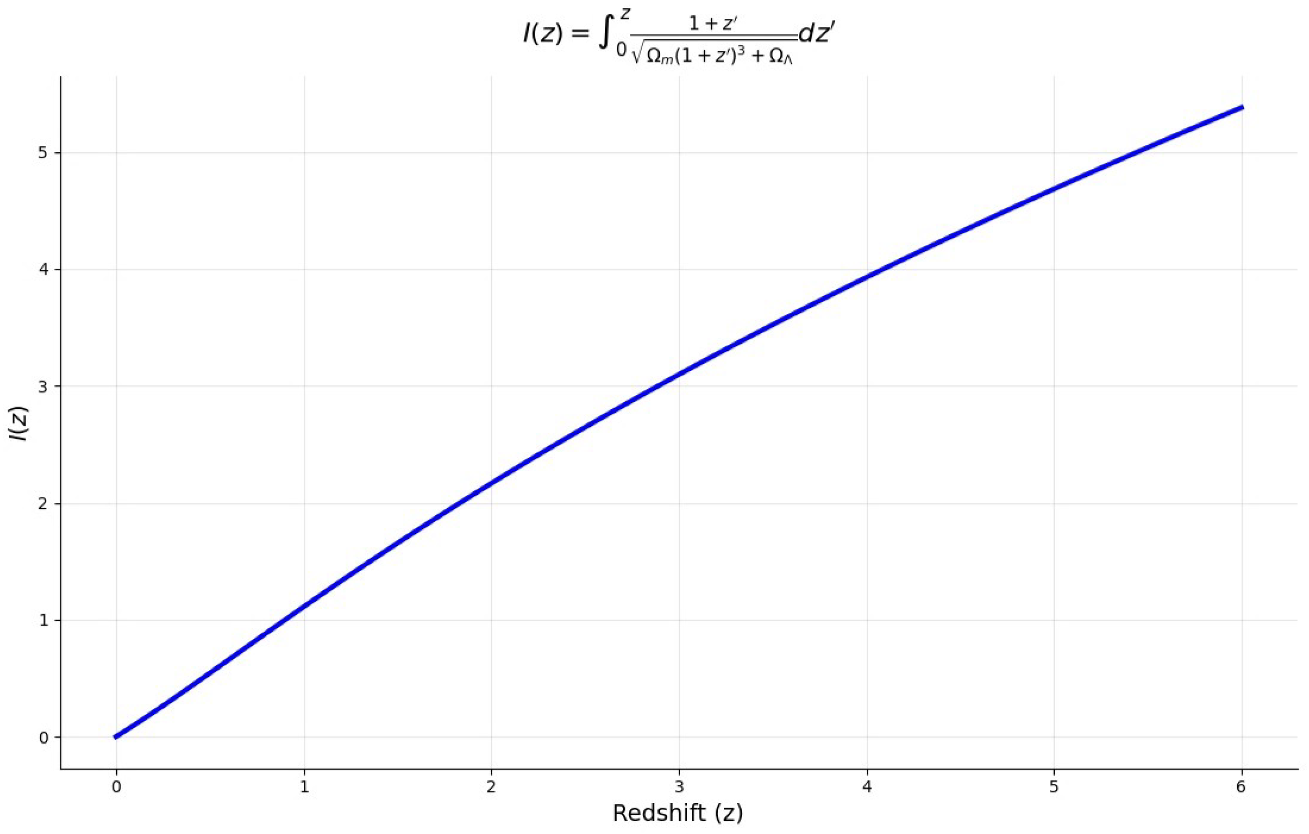
where $H_0=67.4$ km ${\mathrm{s}}^{-1}$${\mathrm{Mpc}}^{-1}$ is the Hubble constant, and ${\mathsf{\Omega }}_m$ = $0.315$ and ${\mathsf{\Omega }}_{\mathsf{\Lambda }}$ = $0.685$ are the matter and dark energy density parameters, values are from [25]. The variation of the dimensionless integral in Equation (4) with redshift is shown in Figure 1.

For subluminal dispersion, $\Delta t_{\mathrm{LIV}}$ is negative, meaning high-energy photons arrive later.

2.2. Intrinsic Spectral Lag Modeling

Even in the absence of LIV, astrophysical sources can exhibit energy-dependent emission timing. GRB pulses often display a hard-to-soft spectral evolution: the spectral peak energy $E_{\mathrm{p}}$ decreases over the pulse duration, causing high-energy photons to be emitted earlier in the pulse and lower-energy photons later [18,19]. This naturally produces a positive intrinsic spectral lag without any propagation effects. Kocevski and Liang [19] demonstrated a direct correlation between the spectral lag and the decay timescale of $E_{\mathrm{p}}$ in GRB pulses, implying that the lag is directly due to the burst’s spectral evolution. In their analysis, as $E_{\mathrm{p}}$ decays through the detector’s bands, each band’s light curve peak is progressively delayed, yielding the observed lag. This provides a physical explanation for the empirical lag’s luminosity relationship: a faster spectral evolution (shorter $E_{\mathrm{p}}$ decay timescale) produces a smaller lag and is associated with higher burst luminosity.

Since the radiation mechanism of gamma-ray bursts leads to a distinct energy dependence in the spectral lag, and in most cases, it is a positive lag (higher-energy photons arrive earlier). To incorporate an intrinsic lag in our model, we assume that in the rest frame of the source, the relationship between photon emission time and photon energy is as follows:

$$t_{\mathrm{emit}}^{\mathrm{rest}}\left(E\right)=t_{\mathrm{p}}+\tau \left[{\left({\displaystyle \frac{E_{\mathrm{p}}}{\mathrm{keV}}}\right)}^{\alpha }-{\left({\displaystyle \frac{E}{\mathrm{keV}}}\right)}^{\alpha }\right],$$

(5)

where $t_{\mathrm{p}}$ represents the emission time corresponding to $E_{\mathrm{p}}$, the peak energy of the spectrum. Photons with energies higher than $E_{\mathrm{p}}$ are emitted earlier, while those with energies lower than $E_{\mathrm{p}}$ are emitted later. In the rest frame of the source, converting Equation (5) yields the time difference of photons arriving at the detector [26]:

$$\Delta t_{\mathrm{int}}^{\mathrm{rest}}=t_{\mathrm{l}}^{\mathrm{rest}}-t_{\mathrm{h}}^{\mathrm{rest}}=\tau \left[{\left({\displaystyle \frac{E_{\mathrm{h}}^{\mathrm{rest}}}{\mathrm{keV}}}\right)}^{\alpha }-{\left({\displaystyle \frac{E_{\mathrm{l}}^{\mathrm{rest}}}{\mathrm{keV}}}\right)}^{\alpha }\right].$$

(6)

By utilizing $\Delta t_{\mathrm{int}}^{\mathrm{obs}}=\Delta t_{\mathrm{int}}^{\mathrm{rest}}(1+z)$ and $E_{\mathrm{rest}}=(1+z)E_{\mathrm{obs}}$, the time delay formula in the rest frame of the source can be transformed into the observer frame [27]:

$$\Delta t_{\mathrm{int}}^{\mathrm{obs}}=\tau \left[{\left({\displaystyle \frac{E_{\mathrm{h}}^{obs}}{\mathrm{keV}}}\right)}^{\alpha }-{\left({\displaystyle \frac{E_{\mathrm{l}}^{obs}}{\mathrm{keV}}}\right)}^{\alpha }\right]{\left(1+z\right)}^{\left(1+\alpha \right)},$$

(7)

where $\tau$ (with dimensions of time) sets the overall amplitude of the intrinsic lag, and $\alpha$ is a dimensionless index governing its energy dependence. Both $\tau >0$ and $\alpha >0$ are expected for the usual hard-to-soft evolution (so that higher E photons arrive earlier). The factor ${(1+z)}^{1+\alpha }$ accounts for cosmological time dilation. Equation (7) effectively assumes that all GRBs in our sample share the same intrinsic lag behavior. Physically, $\tau$ represents the intrinsic lag between two fixed energy scales in the source rest frame. If $\tau$ is on the order of milliseconds, it implies that the emission mechanism in GRBs produces high- versus low-energy photons within a very short timescale.

Equation (7) is highly simplified, resting on the assumption of a simple power-law relation between photon energy and emission time in the source’s rest frame. While it can, in principle, be generalized into a Taylor series or extended with additional parameters, such refinements are not adopted here. This decision is primarily due to the limited sample size and the current lack of observational data for high-energy (GeV to TeV) photons, which would be necessary to constrain a more complex model.

3. Data Sample

Our sample consists of 90 gamma-ray bursts observed by the Neil Gehrels Swift Observatory Burst Alert Telescope (BAT) with known redshifts and well-characterized spectral lags. We directly adopted the spectral lag data published by [28], who analyzed a set of 90 Swift GRBs with redshift determinations. This complete sample provides the foundation for investigating Lorentz invariance violation (LIV) effects. Although the sample of [28] includes some data points with relatively large uncertainties, we decided to use the same sample to enable a direct comparison with their results. Our calculations yield an $E_{QG}$ value of the same order of magnitude as that reported in [28], but our analysis employs a more realistic intrinsic time delay model, which may improve the reliability of the results. The full sample of 90 GRBs is summarized in

Table 1. A positive lag indicates that the photons in the higher-energy band arrive earlier than those in the lower-energy band. Uncertainties are $1\sigma$. Due to differences in redshift measurement methods, observing conditions, and data quality, gamma-ray bursts can have varying numbers of significant figures and different uncertainties in their redshift values. However, the errors introduced during data fitting are negligible, and therefore the uncertainties in redshift have not been provided. Data compiled from [28].

GRB	Redshift (z)	${\mathbf{lag}}_1$ (ms)	${\mathbf{lag}}_2$ (ms)	${\mathbf{lag}}_3$ (ms)	${\mathbf{lag}}_4$ (ms)
050525A	0.606	$-10\pm 8$	$-24\pm 9$	$-13\pm 19$	$-34\pm 17$
050922C	2.198	$+17\pm 77$	$-36\pm 75$	$+55\pm 50$	$+17\pm 127$
051111	1.549	$-329\pm 454$	$-360\pm 416$	$-301\pm 519$	$-775\pm 797$
051221A	0.547	$+0\pm 1$	$+0\pm 2$	$-1\pm 4$	$+0\pm 2$
060206	4.045	$-19\pm 38$	$-120\pm 163$	$-37\pm 286$	$-133\pm 98$
060223A	4.41	$-92\pm 287$	$+320\pm 365$	$-127\pm 283$	$-205\pm 339$
060418	1.490	$-18\pm 77$	$+12\pm 213$	$-176\pm 445$	$-35\pm 142$
060502A	1.51	$+235\pm 514$	$-1571\pm 768$	$+753\pm 872$	$-381\pm 979$
060814	0.84	$-161\pm 155$	$-30\pm 261$	$-411\pm 301$	$-297\pm 289$
060908	1.8836	$+23\pm 144$	$-279\pm 102$	$-12\pm 91$	$-80\pm 132$
060912A	0.937	$+17\pm 55$	$+57\pm 63$	$+106\pm 124$	$+110\pm 105$
060927	5.6	$-69\pm 142$	$+44\pm 131$	$-39\pm 72$	$-50\pm 109$
061007	1.261	$-3\pm 20$	$-6\pm 14$	$-58\pm 39$	$-65\pm 45$
061121	1.314	$-11\pm 10$	$-16\pm 19$	$+11\pm 22$	$-28\pm 17$
061222A	2.088	$-17\pm 24$	$-19\pm 18$	$-24\pm 22$	$-54\pm 31$
070506	2.31	$+21\pm 267$	$-765\pm 619$	$-169\pm 429$	$-487\pm 575$
070508	0.82	$-9\pm 6$	$-4\pm 13$	$+1\pm 11$	$-21\pm 13$
071010B	0.947	$-129\pm 125$	$-109\pm 209$	$+157\pm 375$	$-348\pm 353$
071020	2.142	$-13\pm 10$	$-19\pm 13$	$-5\pm 12$	$-43\pm 11$
071117	1.331	$-61\pm 57$	$-33\pm 57$	$+0\pm 25$	$-181\pm 65$
080319B	0.937	$-7\pm 7$	$-10\pm 10$	$+8\pm 19$	$-22\pm 12$
080319C	1.95	$-70\pm 80$	$+7\pm 109$	$-87\pm 126$	$-161\pm 87$
080411	1.03	$-33\pm 15$	$-12\pm 20$	$-13\pm 23$	$-62\pm 34$
080413A	2.433	$-61\pm 49$	$+15\pm 56$	$+0\pm 58$	$-27\pm 67$
080413B	1.10	$-114\pm 71$	$+120\pm 62$	$-71\pm 106$	$-117\pm 72$
080605	1.6398	$-34\pm 16$	$-30\pm 25$	$+5\pm 32$	$-66\pm 19$
080607	3.036	$+6\pm 61$	$-19\pm 86$	$-37\pm 39$	$-38\pm 38$
081221	2.26	$-56\pm 57$	$+30\pm 71$	$-63\pm 97$	$-165\pm 57$
081222	2.77	$-16\pm 43$	$-66\pm 51$	$+25\pm 77$	$+26\pm 108$
090424	0.544	$-1\pm 11$	$+15\pm 19$	$-13\pm 25$	$-22\pm 23$
090618	0.54	$-78\pm 89$	$-49\pm 109$	$-153\pm 208$	$-342\pm 291$
090715B	3.00	$+346\pm 219$	$-518\pm 253$	$-26\pm 431$	$+83\pm 310$
090812	2.452	$-117\pm 234$	$-103\pm 172$	$+25\pm 91$	$+21\pm 165$
091018	0.971	$-47\pm 97$	$-118\pm 81$	$+234\pm 203$	$+148\pm 191$
091020	1.71	$+161\pm 213$	$+399\pm 294$	$-9\pm 514$	$+356\pm 703$
091029	2.752	$+293\pm 415$	$-250\pm 778$	$-591\pm 858$	$-314\pm 852$
100615A	1.398	$-42\pm 76$	$-87\pm 66$	$+10\pm 260$	$-104\pm 125$
100621A	0.542	$-209\pm 103$	$-509\pm 290$	$-108\pm 907$	$-655\pm 850$
100704A	3.6	$-504\pm 460$	$+163\pm 407$	$-466\pm 263$	$-334\pm 285$
100728A	1.567	$-15\pm 36$	$-30\pm 43$	$-37\pm 42$	$-29\pm 36$
100814A	1.44	$-247\pm 115$	$-47\pm 149$	$-43\pm 251$	$+94\pm 353$
100816A	0.8034	$-21\pm 38$	$-11\pm 42$	$-76\pm 150$	$-79\pm 94$
100906A	1.727	$-30\pm 96$	$+14\pm 49$	$-129\pm 131$	$+51\pm 122$
101219A	0.718	$-3\pm 9$	$+6\pm 11$	$-1\pm 30$	$-9\pm 33$
110422A	1.77	$-2\pm 30$	$-20\pm 59$	$+7\pm 27$	$-52\pm 36$
110503A	1.613	$-71\pm 174$	$-41\pm 143$	$-51\pm 85$	$-119\pm 150$
110715A	0.82	$-23\pm 15$	$-18\pm 23$	$-48\pm 27$	$-84\pm 31$
110731A	2.83	$+4\pm 15$	$+2\pm 26$	$-25\pm 16$	$-20\pm 17$
120119A	1.728	$-7\pm 81$	$-15\pm 114$	$+22\pm 126$	$+10\pm 79$
120326A	1.798	$-18\pm 310$	$-472\pm 154$	$+680\pm 288$	$-200\pm 450$
120327A	2.81	$+5\pm 138$	$-60\pm 111$	$-150\pm 130$	$+2\pm 142$
120712A	4.15	$+123\pm 355$	$-216\pm 435$	$-198\pm 360$	$-2\pm 227$
120811C	2.671	$-383\pm 200$	$+44\pm 374$	$-284\pm 268$	$-638\pm 281$
121128A	2.20	$-11\pm 21$	$-12\pm 14$	$+8\pm 20$	$-4\pm 25$
130427A	0.34	$-10\pm 11$	$-6\pm 8$	$+7\pm 21$	$-15\pm 29$
130514A	3.6	$+311\pm 535$	$-294\pm 452$	$+357\pm 636$	$+75\pm 263$
130610A	2.092	$-145\pm 570$	$+309\pm 722$	$-329\pm 924$	$-1285\pm 777$
130907A	1.238	$+0\pm 8$	$-3\pm 9$	$-12\pm 8$	$-16\pm 11$
131030A	1.293	$-103\pm 39$	$+84\pm 62$	$-40\pm 39$	$-101\pm 51$
140206A	2.73	$-62\pm 14$	$-25\pm 21$	$-9\pm 15$	$-72\pm 17$
140213A	1.2076	$+8\pm 44$	$-12\pm 41$	$+52\pm 63$	$+66\pm 54$
140419A	3.956	$+12\pm 503$	$-84\pm 240$	$-117\pm 206$	$-114\pm 182$
140512A	0.725	$-56\pm 93$	$-53\pm 151$	$+119\pm 381$	$-77\pm 427$
141220A	1.3195	$+28\pm 99$	$-37\pm 83$	$+66\pm 68$	$+77\pm 70$
150206A	2.087	$-34\pm 49$	$-24\pm 124$	$+18\pm 57$	$-22\pm 64$
150301B	1.5169	$-242\pm 362$	$+346\pm 187$	$+13\pm 212$	$+95\pm 171$
150314A	1.758	$-28\pm 24$	$-4\pm 77$	$-43\pm 35$	$-61\pm 44$
150403A	2.06	$-40\pm 111$	$-19\pm 151$	$-173\pm 129$	$-212\pm 97$
151021A	2.330	$+12\pm 452$	$-643\pm 621$	$+857\pm 1004$	$+408\pm 557$
160131A	0.97	$-131\pm 298$	$-84\pm 306$	$-205\pm 217$	$-323\pm 384$
161117A	1.549	$-102\pm 184$	$-164\pm 294$	$-10\pm 256$	$-418\pm 256$
170202A	3.645	$+57\pm 103$	$-48\pm 90$	$+20\pm 87$	$-34\pm 92$
170705A	2.010	$-17\pm 60$	$+38\pm 120$	$-60\pm 87$	$-78\pm 77$
180314A	1.445	$-335\pm 613$	$-309\pm 548$	$-764\pm 604$	$-1290\pm 607$
180325A	2.25	$-12\pm 157$	$-87\pm 90$	$-112\pm 104$	$-269\pm 159$
180720B	0.654	$+0\pm 23$	$-8\pm 49$	$+10\pm 42$	$-27\pm 36$
181020A	2.938	$-183\pm 165$	$-52\pm 135$	$+71\pm 133$	$-117\pm 217$
190106A	1.86	$-74\pm 112$	$+28\pm 188$	$-25\pm 221$	$+6\pm 145$
190114C	0.42	$+3\pm 4$	$-5\pm 6$	$+2\pm 15$	$+6\pm 17$
190324A	1.1715	$-97\pm 120$	$-113\pm 97$	$+16\pm 124$	$-62\pm 65$
191221B	1.148	$-48\pm 55$	$-17\pm 84$	$-62\pm 88$	$-55\pm 152$
200829A	1.25	$-28\pm 32$	$-1\pm 27$	$-73\pm 34$	$-161\pm 41$
201020A	2.903	$-437\pm 343$	$-921\pm 613$	$+770\pm 715$	$-508\pm 1052$
201104B	1.954	$-15\pm 23$	$+28\pm 36$	$+5\pm 36$	$+20\pm 47$
201216C	1.10	$-74\pm 225$	$-65\pm 102$	$+196\pm 192$	$-22\pm 222$
210411C	2.826	$-161\pm 150$	$+79\pm 176$	$-80\pm 93$	$-137\pm 164$
210610B	1.13	$-285\pm 390$	$+108\pm 196$	$-136\pm 418$	$-446\pm 297$
210619B	1.937	$-14\pm 16$	$-19\pm 24$	$+1\pm 18$	$-44\pm 24$
210822A	1.736	$-2\pm 7$	$+3\pm 10$	$+3\pm 11$	$+0\pm 16$
220101A	4.61	$-79\pm 73$	$-23\pm 49$	$-26\pm 69$	$-19\pm 73$

, with redshifts ranging from $z=0.34$ to $z=5.6$, providing a broad lever-arm for probing potential LIV effects.

Each GRB’s prompt emission light curve was divided by [28] into four fixed observer-frame energy bands within the Swift/BAT range: $E_1:100$–137.5 keV, $E_2:137.5$–175 keV, $E_3:175$–212.5 keV, and $E_4:212.5$–250 keV. For convenience, we used the arithmetic mean of the energy in each energy band as the representative energy during the calculation process. Cross-correlation analysis was used to measure the time lag between different bands. For each burst we have up to four lag measurements: ${\mathrm{lag}}_1$ between $E_1$ and $E_2$, ${\mathrm{lag}}_2$ between $E_2$ and $E_3$, ${\mathrm{lag}}_3$ between $E_3$ and $E_4$, and ${\mathrm{lag}}_4$ between $E_1$ and $E_4$. These lags (in milliseconds) with 1$\sigma$ uncertainties are listed in Table 1. Many of the measured lags are consistent with zero within errors, but some bursts show significantly non-zero lags. Our analysis will account for both positive and negative lag values in a unified fit.

4. Methodology

This section details the Bayesian inference framework and Markov Chain Monte Carlo (MCMC) implementation used to constrain the free parameters of the time delay model. This includes posterior probability construction, a preliminary fitting stage to initialize sampling, the overall sampling strategy, and result post-processing. Prior to the full Bayesian MCMC analysis, a non-linear least-squares fitting procedure was employed to obtain a preliminary estimate of the model parameters. This step served two primary purposes: (1) to determine suitable initial values for the MCMC chains, and (2) to inform the placement of physically reasonable and computationally efficient bounds on the parameter space. By identifying a region of high likelihood in advance, this approach significantly accelerates the convergence of the subsequent MCMC sampling and helps avoid prolonged exploration of low-probability areas. The results from this preliminary fit were used solely for initialization and boundary definition; the final parameter constraints and uncertainties are derived exclusively from the full posterior distribution sampled by the MCMC process.

4.1. Bayesian Inference Framework

Bayesian inference was employed to constrain the three free parameters of the time delay model, denoted as the parameter vector $\theta =\{E_{\mathrm{QG}},\tau ,\alpha \}$. The posterior probability distribution of the parameters, conditioned on observational data D, is given by Bayes’ theorem:

$$\mathcal{P}\left(\theta \right|D)\propto \mathcal{L}(D\left|\theta \right)·\pi \left(\theta \right)$$

(8)

where $\mathcal{L}\left(D\right|\theta )$ represents the likelihood function quantifying the agreement between model predictions and observations, and $\pi \left(\theta \right)$ denotes the prior probability distribution encoding a priori physical constraints on the parameters.

Likelihood Function

A Gaussian likelihood function was adopted, under the assumption that the measurement uncertainties of the observed time delays follow normal distributions. The log-likelihood function, used for computational efficiency, is expressed as:

$$ln\mathcal{L}=-{\displaystyle \frac{1}{2}}\sum _{i=1}^N{\left({\displaystyle \frac{\Delta t_{\mathrm{obs},\mathrm{i}}-\Delta t_{\mathrm{model},\mathrm{i}}\left(\theta \right)}{{\sigma }_{\Delta t_i}}}\right)}^2-{\displaystyle \frac{1}{2}}\sum _{i=1}^{N}ln\left(2\pi {\sigma }_{\Delta t_i}^2\right)$$

(9)

where N is the number of observational data points, $\Delta t_{\mathrm{obs},\mathrm{i}}$ is the i-th observed time delay, $\Delta t_{\mathrm{model},\mathrm{i}}\left(\theta \right)$ is the corresponding model-predicted time delay, and ${\sigma }_{\Delta t_i}$ is the measurement uncertainty of $\Delta t_{\mathrm{obs},\mathrm{i}}$.

To enforce physical consistency, any parameter combination $\theta$ falling outside the predefined constraint ranges returns a log-likelihood value of $-\infty$ (hard constraint).

4.2. Model Fitting Procedure

Prior Distributions

The initial guesses and ranges for the parameters are listed in

Table 2. Initial parameter guesses and upper and lower bounds for nonlinear fitting.

	${\mathit{E}}_{\mathit{QG}}$	$\mathit{\tau }$	$\mathit{\alpha }$
initial guesses	${10}^{15}$ GeV	${10}^{-3}$ s	$0.5$
lower bounds	${10}^6$ GeV	$-10$ s	$-5$
upper bounds	${10}^{20}$ GeV	10 s	5

, and the preliminary fitting results are presented in

Table 3. Parameter estimation results from nonlinear fitting.

	Fitting Result	68% CI
$E_{QG}$	$1.04\times {10}^{15}$ GeV	$[9.67\times {10}^{14},1.22\times {10}^{15}]$ GeV
$\tau$	$4.94\times {10}^{-3}$ s	$[4.14\times {10}^{-4},6.78\times {10}^{-3}]$ s
$\alpha$	0.411	$[0.384,0.472]$
${\chi }^2/\mathrm{dof}$	307.1/357 = 0.860
p-value	0.974

. We initially set the parameter ranges relatively wide to avoid missing physically plausible solutions. Subsequently, preliminary parameter estimates were obtained through nonlinear fitting, with 68% CI provided by bootstrap uncertainty estimation.

Based on these estimates, the constraint ranges were further narrowed to ensure physical reasonableness and improve sampling efficiency. The specific parameter settings are as follows:

• Quantum gravity energy scale ($E_{QG}$): A log-uniform prior was imposed over the range ${10}^6\le E_{\mathrm{QG}}\le {10}^{20}\mathrm{GeV}$, such that $\pi \left(E_{\mathrm{QG}}\right)\propto 1/E_{\mathrm{QG}}$. This prior accounts for the wide dynamic range of $E_{QG}$ expected in quantum gravity scenarios.
• Intrinsic time delay parameter ($\tau$): A log-uniform prior was applied over the interval ${10}^{-4}\le \tau \le {10}^{-2}\mathrm{s}$, with $\pi \left(\tau \right)\propto 1/\tau$ reflecting the scale-dependent nature of the intrinsic time delay effect.
• Energy dependence exponent ($\alpha$): A uniform prior was adopted over $0\le \alpha \le 1.0$, i.e., $\pi \left(\alpha \right)=\mathrm{constant}$, as no strong a priori preference exists for specific values within this range.

The total log-prior is the sum of the log-priors of individual parameters. For any parameter outside its predefined range, the log-prior is set to $-\infty$. It should be emphasized that the refined constraint ranges are derived from nonlinear fitting results, which ensures that the subsequent MCMC sampling is focused on the physically plausible parameter space, balancing the completeness of exploration and computational efficiency.

4.3. MCMC Implementation

The ensemble sampler emcee [29] was used to sample the posterior probability distribution, leveraging its affine-invariant property to efficiently explore high-dimensional parameter spaces without manual tuning of proposal distributions.

4.3.1. Initialization Strategy

A two-step initialization procedure was implemented to ensure the sampler starts from physically meaningful parameter values:

• Maximum A Posteriori (MAP) Estimation: The MAP point of the posterior distribution was first obtained by minimizing the negative log-posterior function, using the L-BFGS-B optimization algorithm (scipy.optimize.minimize). Multiple initial guesses were tested to avoid convergence to local minima, ensuring the final MAP estimate is representative of the global posterior mode.
• Walker Initialization: 32 walkers (ensemble members) were initialized by adding controlled perturbations to the MAP estimate. For $E_{QG}$ and $\tau$, perturbations were applied in logarithmic space to account for their wide dynamic ranges; for $\alpha$, perturbations were added in linear space. All walker positions were clipped to the predefined parameter ranges to enforce hard constraints from the outset.

4.3.2. Post-Processing

After sampling, the following post-processing steps were performed to extract robust parameter constraints:

• Flat Sample Extraction: Chains from all walkers were concatenated (after discarding the burn-in phase) to generate a flat sample of posterior parameter values.
• Goodness of Fit Evaluation: The reduced chi-squared statistic ${\chi }_{\mathrm{red}}^2={\chi }^2/\mathrm{dof}$ was calculated to quantify the agreement between the model and observations, where ${\chi }^2={\sum }_{i=1}^N{\left({\displaystyle \frac{\Delta t_{\mathrm{obs},\mathrm{i}}-\Delta t_{\mathrm{model},\mathrm{i}}\left({\theta }_{\mathrm{best}}\right)}{{\sigma }_{\Delta t}}}\right)}^2$, ${\theta }_{\mathrm{best}}$ is the best-fit parameter set (MAP estimate), and $\mathrm{dof}=N-3$ is the number of degrees of freedom (number of data points minus the number of free parameters).

5. Results

The fitting procedure converged to a solution with a reduced chi-squared value of ${\chi }_{\nu }^2=0.889$ (for 357 degrees of freedom). The MAP are $E_{\mathrm{QG}}=8.96\times {10}^{14}\mathrm{GeV}$, $\tau =2.64\times {10}^{-3}\mathrm{s}$, $\alpha =0.53$. Based on MCMC simulation, the posterior distribution is skewed; therefore, we report the 95% Highest Density Interval (HDI) as the interval estimate. The 95% HDI and the median of the parameters are shown in the

Table 4. The 95% HDI and median values of the fitted parameters.

	95% HDI	Median Value
$E_{QG}$	$[6.67\times {10}^{14},1.90\times {10}^{15}]$ GeV	$1.15\times {10}^{15}$ GeV
$\tau$	$[1.17\times {10}^{-3},9.52\times {10}^{-3}]$ s	$4.47\times {10}^{-3}$ s
$\alpha$	$[0.29,0.61]$	0.43

.

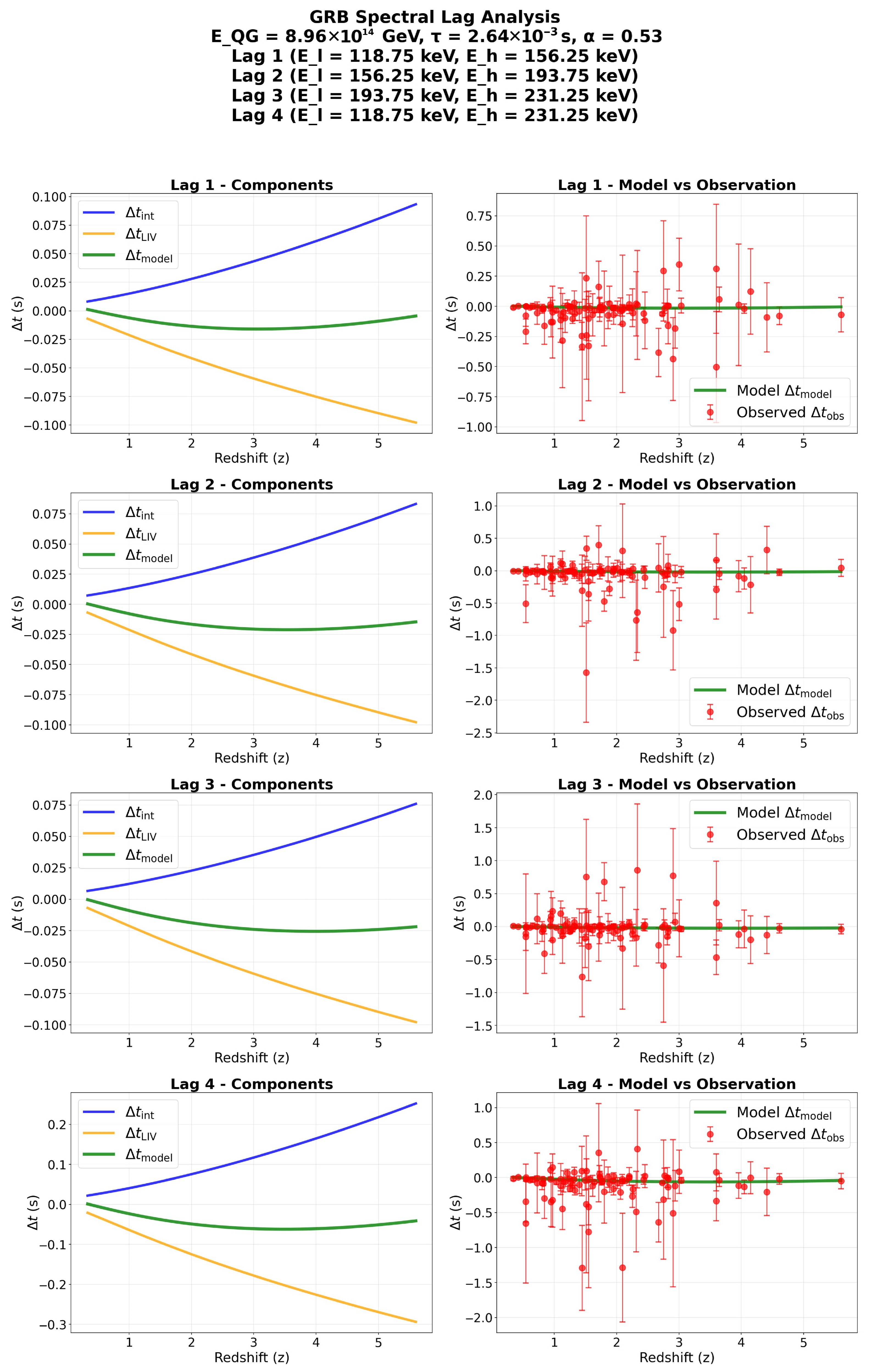
The first column of subplots in Figure 2 presents the time delay curves induced by the LIV effect and the intrinsic time delay effect under the selected MAP parameters, along with the fitted curve of the total time delay. The second column of subplots in Figure 2 provides a comparison between the fitted curves and the observed values. Specifically, the subplots in the first column, respectively, show the comparison between the components attributed to the LIV effect and the intrinsic time delay effect for $la{g}_1$ to $la{g}_4$, while the subplots in the second column display the comparison between the fitted and observed values for $la{g}_1$ to $la{g}_4$.

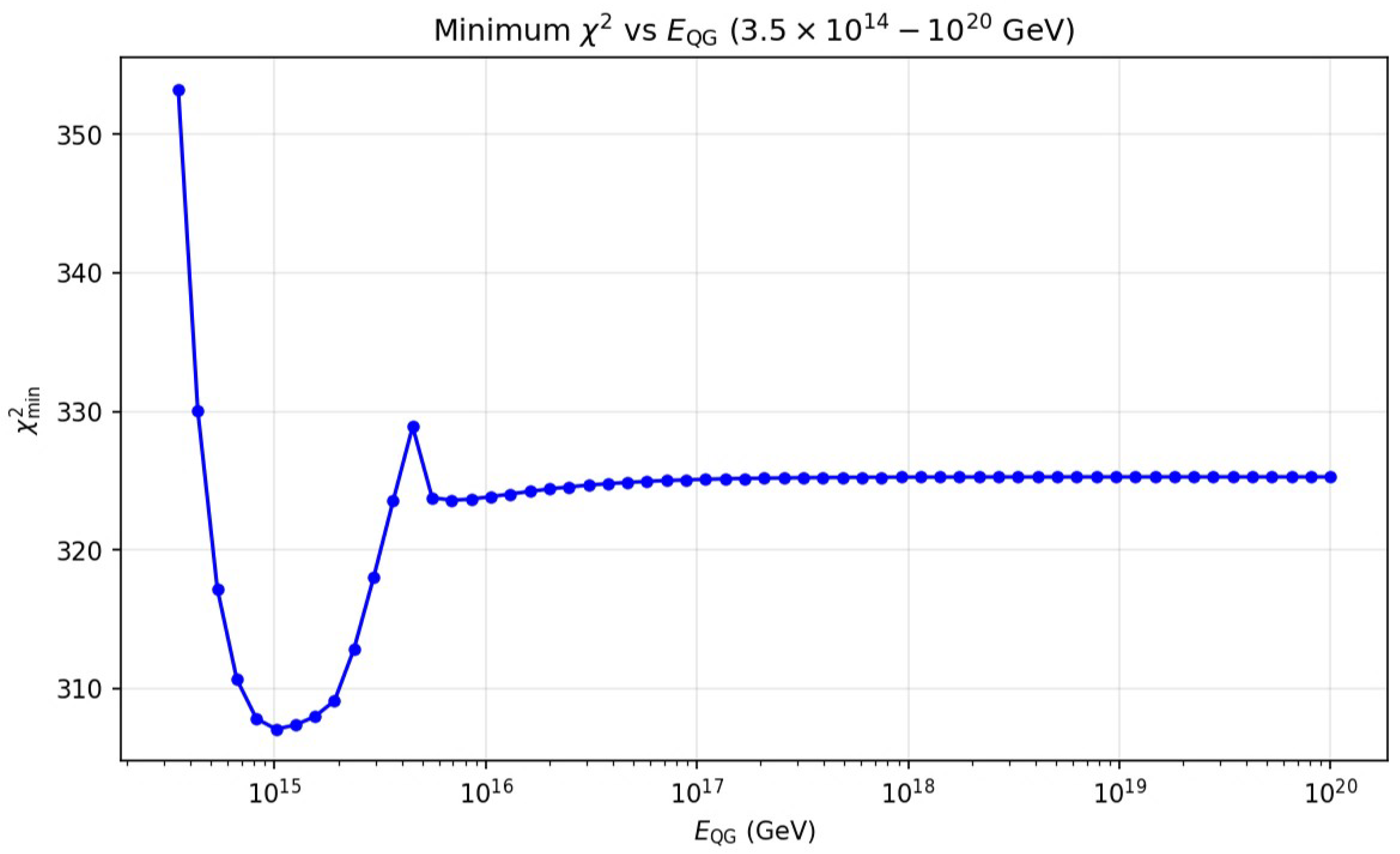
Figure 3 shows the variation of ${\chi }^2$ with $E_{\mathrm{QG}}$. We restrict the value range of $E_{\mathrm{QG}}$ to $[3.5\times {10}^{14},{10}^{20}]$ GeV. The curve is constructed by fixing each value of $E_{\mathrm{QG}}$ and minimizing ${\chi }^2$ over the free parameters $\tau$ and $\alpha$ in the intrinsic time delay model. Interestingly, the ${\chi }^2$ value corresponding to the MAP parameters is larger than that obtained from the preliminary fit. This behavior arises because the posterior distribution of the parameters may not follow a unimodal Gaussian distribution. The MAP estimate, which accounts for the full probability mass over the parameter space, is generally regarded as statistically more robust than the least-squares point estimate. We therefore adopt the MAP result as our preferred measurement. In particular, we take the MAP estimate $E_{\mathrm{QG}}=8.96\times {10}^{14}\mathrm{GeV}$ derived from MCMC as our best-fit result, with the corresponding minimum ${\chi }_{\mathrm{MAP}}^2=317.3$.

When $E_{QG}\ge {10}^{20}$ GeV, corresponding to the plateau of ${\chi }^2$, which corresponds to the standard LI scenario (no LIV effects), the profile likelihood ${\chi }^2$ approaches a constant value ${\chi }_{\infty }^2=325.3$. The improvement in the goodness of fit is calculated as:

$$\Delta {\chi }^2={\chi }_{\infty }^2-{\chi }_{\mathrm{MAP}}^2=8,$$

(10)

with $\Delta \mathrm{dof}=1$ (the LIV model introduces one additional free parameter $E_{\mathrm{QG}}$ compared to the LI model). This $\Delta {\chi }^2$ value corresponds to a statistical significance of approximately $2.8\sigma$, indicating a preference for the LIV model over the strict Lorentz-invariant hypothesis.

The intrinsic lag parameters $\tau$ and $\alpha$ are well constrained and positive, consistent with a universal intrinsic hard-to-soft lag among all GRBs in our sample. We regard the derived value $E_{\mathrm{QG}}=6.67\times {10}^{14}$ GeV as the lower bound on the quantum gravity energy scale at linear order. This value is on the same order of magnitude as, but slightly higher than, recent limits obtained by [28] using similar data.

The small intrinsic lag timescale τ∼$1\times {10}^{-3}$ s (rest-frame $\sim$0.5 ms for a typical z$\sim$1 burst) implies that the emission mechanism in GRBs produces high- versus low-energy photons within a very short timescale. This timescale is much shorter than naive expectations from light-travel geometry across a relativistically expanding shell. In the following, we explore the physical interpretation of this short lag.

6. Physical Interpretation and Discussion

Previous studies either assumed the intrinsic time delay to be a constant [9] or modeled it as a function of energy alone [26]. In our work, we assume the intrinsic time delay to be a function that depends on both energy and redshift, and we further assume that this intrinsic time delay function applies to all gamma-ray bursts [27]. The fitted intrinsic lag timescale of τ$\sim$1 × 10⁻³ s is intriguingly short. To put this in context, consider the angular (curvature) timescale in GRB emission. Photons emitted simultaneously from different parts of a relativistically expanding spherical shell will reach the observer at different times due to path length differences. For a shell at radius R moving with bulk Lorentz factor $\Gamma$, the curvature (or angular) timescale is approximately

$$t_{\mathrm{ang}}\approx {\displaystyle \frac{R}{2c{\Gamma }^2}}.$$

(11)

This timescale represents the time delay between photons emitted on-axis and those emitted from the edge of the visible emission region (at an angle of $1/\Gamma$ relative to the line of sight). If R∼${10}^{14}$ cm and $\Gamma$∼300, one finds $t_{\mathrm{ang}}$∼30 ms, an order of magnitude larger than the observed $\tau$. Even with $\Gamma$∼1000 and R∼$5\times {10}^{13}$ cm, $t_{\mathrm{ang}}$ would be on the order of a few milliseconds. The fact that $\tau \ll t_{\mathrm{ang}}$ suggests that not all parts of the shell radiate simultaneously—otherwise the emission would be smeared over at least tens of milliseconds. Instead, it implies that the effective emitting region is much narrower. We can define a dimensionless scaling factor $f\equiv {\tau }_{\mathrm{rest}}/t_{\mathrm{ang}}^{\mathrm{rest}}$, where ${\tau }_{\mathrm{rest}}=\tau /(1+z)$ and $t_{\mathrm{ang}}^{\mathrm{rest}}=t_{\mathrm{ang}}/(1+z)$. Using typical parameters yields $f$∼0.03–0.1. A more likely interpretation is that only a fraction of the shell’s surface is active at any given time, effectively reducing the angular spread of emitting regions and thus the observed pulse widths and lags by a factor f.

One scenario capturing this idea is the patchy shell model [30], which proposed that the GRB outflow has an intrinsic angular structure, with energy dissipation occurring in localized patches rather than uniformly across the whole jet. An observer would see emission from only a small patch (angular size ${\theta }_{\mathrm{patch}}<1/\Gamma$) at any given moment. Each patch produces a very fast, sharp pulse because the curvature delay is short over that small angle. Our finding of $f$∼0.1 or smaller is consistent with a picture in which only ∼10% or less of the emitting area contributes coherently to a given spike of emission.

Another related concept is that of relativistic turbulence or mini-jets within the jet. In Poynting-flux-dominated outflows or magnetic reconnection models, small blobs or filaments of plasma move relativistically within the jet and emit gamma rays into a narrow cone inside the overall jet cone. This mini-jet model can shorten variability timescales by a factor corresponding to the relative Lorentz factor of the blob. Refs. [31,32] showed that internal motions with Lorentz factor ${\Gamma }^{\prime }$ of a few can reduce pulse widths and lags by factors of several. Our measured $f\approx 0.03$–$0.1$ supports models in which the emitting region is anisotropic or temporally intermittent on angular scales much less than $1/\Gamma$.

Other physical processes may also contribute. For instance, the intrinsic lag could reflect the cooling time of high-energy electrons or radiative transfer effects in a dense photosphere. In synchrotron models, high-energy photons come from freshly accelerated electrons which then cool, emitting lower-energy photons slightly later. If the synchrotron cooling time is of order milliseconds in the comoving frame, this could yield an intrinsic lag. Without committing to one mechanism, we note that τ∼${10}^{-3}$ s in the source frame corresponds to length scales $c\tau$$\sim$$3\times {10}^7$ cm, much smaller than the emission radius, suggesting the lag is not due to large-scale structure but rather a local process.

7. Conclusions

We have analyzed spectral lag data from 90 GRBs to test Lorentz invariance violation and measure intrinsic emission delays. By fitting a combined model of LIV-induced and intrinsic spectral lags to 360 lag measurements, we found that the MAP value of the linear-order quantum gravity energy scale is located near $8.96\times {10}^{14}$ GeV. This energy scale lies between the electroweak scale and the Planck scale, potentially providing an observational window into the energy regime where certain quantum gravity theories (such as string theory and loop quantum gravity) predict phenomena such as extra dimensions or spacetime foam. This finding is of significant importance, as it indicates an energy range that could, in principle, be probed by future ultra-high-energy astronomical observations. The intrinsic spectral lag can be described by $\Delta t_{\mathrm{int}}=\tau \left[{\left({\displaystyle \frac{E_h}{1\mathrm{keV}}}\right)}^{\alpha }-{\left({\displaystyle \frac{E_l}{1\mathrm{keV}}}\right)}^{\alpha }\right]{(1+z)}^{1+\alpha }$ with $\tau \approx 2.64\times {10}^{-3}$ s and $\alpha \approx 0.53$, implying a millisecond-scale intrinsic lag in GRBs. This approach differs from previous studies which assumed the intrinsic time delay to be either constant or depends solely on energy. The intrinsic lag timescale is much shorter than the curvature timescale for typical GRB parameters, suggesting that only a fraction of the emitting region is active at any given time or that relativistic substructure within the jet shortens variability timescales. Future observations with a broader energy range, including GeV–TeV photons, and a larger GRB sample will improve the sensitivity to LIV and help refine intrinsic lag models.

References

1. Amelino-Camelia, G.; Ellis, J.; Mavromatos, N.E.; Nanopoulos, D.V.; Sarkar, S. Tests of quantum gravity from observations of γ-ray bursts. Nature 1998, 393, 763–765. [Google Scholar] [CrossRef]
2. Desai, S. Astrophysical and Cosmological Searches for Lorentz Invariance Violation. In Recent Progress on Gravity Tests: Challenges and Future Perspectives; Bambi, C., Cárdenas-Avendaño, A., Eds.; Springer Nature: Singapore, 2024; pp. 433–463. [Google Scholar] [CrossRef]
3. Stecker, F. Constraints on Lorentz invariance violating quantum gravity and large extra dimensions models using high energy γ-ray observations. Astropart. Phys. 2003, 20, 85–90. [Google Scholar] [CrossRef][Green Version]
4. Alan Kostelecký, V.; Potting, R. CPT and strings. Nucl. Phys. B 1991, 359, 545–570. [Google Scholar] [CrossRef]
5. Kostelecký, V.A.; Potting, R. CPT, strings, and meson factories. Phys. Rev. D 1995, 51, 3923–3935. [Google Scholar] [CrossRef]
6. Mattingly, D. Modern Tests of Lorentz Invariance. Living Rev. Relativ. 2005, 8, 5. [Google Scholar] [CrossRef]
7. Tasson, J.D. What do we know about Lorentz invariance? Rep. Prog. Phys. 2014, 77, 062901. [Google Scholar] [CrossRef] [PubMed]
8. Brahma, S.; Chen, C.Y.; Yeom, D.h. Testing Loop Quantum Gravity from Observational Consequences of Nonsingular Rotating Black Holes. Phys. Rev. Lett. 2021, 126, 181301. [Google Scholar] [CrossRef]
9. Ellis, J.; Mavromatos, N.E.; Nanopoulos, D.V.; Sakharov, A.S.; Sarkisyan, E.K.G. Robust limits on Lorentz violation from gamma-ray bursts. Astropart. Phys. 2006, 25, 402–411. [Google Scholar] [CrossRef]
10. Jacob, U.; Piran, T. Lorentz-violation-induced arrival delays of cosmological particles. J. Cosmol. Astropart. Phys. 2008, 2008, 031. [Google Scholar] [CrossRef]
11. Pavlopoulos, T.G. Are we observing Lorentz violation in gamma ray bursts? [rapid communication]. Phys. Lett. B 2005, 625, 13–18. [Google Scholar] [CrossRef]
12. Kostelecký, V.A.; Mewes, M. Electrodynamics with Lorentz-violating operators of arbitrary dimension. Phys. Rev. D—Part. Fields Gravit. Cosmol. 2009, 80, 015020. [Google Scholar] [CrossRef]
13. Abdo, A.A.; Ackermann, M.; Arimoto, M.; Asano, K.; Atwood, W.B.; Axelsson, M.; Baldini, L.; Ballet, J.; Band, D.L.; Barbiellini, G.; et al. Fermi Observations of High-Energy Gamma-Ray Emission from GRB 080916C. Science 2009, 323, 1688. [Google Scholar] [CrossRef]
14. Vasileiou, V.; Jacholkowska, A.; Piron, F.; Bolmont, J.; Couturier, C.; Granot, J.; Stecker, F.W.; Cohen-Tanugi, J.; Longo, F. Constraints on Lorentz invariance violation from Fermi-Large Area Telescope observations of gamma-ray bursts. Phys. Rev. D—Part. Fields Gravit. Cosmol. 2013, 87, 122001. [Google Scholar] [CrossRef]
15. Kislat, F.; Krawczynski, H. Search for anisotropic Lorentz invariance violation with γ-rays. Phys. Rev. D 2015, 92, 045016. [Google Scholar] [CrossRef]
16. Liu, Z.K.; Zhang, B.B.; Meng, Y.Z. Spectral Lag Transition of 32 Fermi Gamma-Ray Bursts and Their Application on Constraining Lorentz Invariance Violation. Astrophys. J. 2022, 935, 79. [Google Scholar] [CrossRef]
17. Kostelecký, V.A.; Mewes, M. Astrophysical Tests of Lorentz and CPT Violation with Photons. Astrophys. J. Lett. 2008, 689, L1. [Google Scholar] [CrossRef]
18. Norris, J.P.; Marani, G.F.; Bonnell, J.T. Connection between Energy-dependent Lags and Peak Luminosity in Gamma-Ray Bursts. Astrophys. J. 2000, 534, 248–257. [Google Scholar] [CrossRef]
19. Kocevski, D.; Liang, E. The Connection between Spectral Evolution and Gamma-Ray Burst Lag. Astrophys. J. 2003, 594, 385–389. [Google Scholar] [CrossRef]
20. Addazi, A.; Alvarez-Muniz, J.; Alves Batista, R.; Amelino-Camelia, G.; Antonelli, V.; Arzano, M.; Asorey, M.; Atteia, J.L.; Bahamonde, S.; Bajardi, F.; et al. Quantum gravity phenomenology at the dawn of the multi-messenger era—A review. Prog. Part. Nucl. Phys. 2022, 125, 103948. [Google Scholar] [CrossRef]
21. Gao, H.; Wu, X.F.; Mészáros, P. Cosmic transients test einstein’s equivalence principle out to GeV energies. Astrophys. J. 2015, 810, 121. [Google Scholar] [CrossRef]
22. Wei, J.J.; Gao, H.; Wu, X.F.; Mészáros, P. Testing Einstein’s Equivalence Principle With Fast Radio Bursts. Phys. Rev. Lett. 2015, 115, 261101. [Google Scholar] [CrossRef]
23. Wei, J.J.; Wu, X.F.; Zhang, B.B.; Shao, L.; Mészáros, P.; Kostelecký, V.A. Constraining Anisotropic Lorentz Violation via the Spectral-lag Transition of GRB 160625B. Astrophys. J. 2017, 842, 115. [Google Scholar] [CrossRef]
24. Zhu, J.; Ma, B.Q. Lorentz-violation-induced arrival time delay of astroparticles in Finsler spacetime. Phys. Rev. D 2022, 105, 124069. [Google Scholar] [CrossRef]
25. Planck Collaboration; Aghanim, N.; Akrami, Y.; Ashdown, M.; Aumont, J.; Baccigalupi, C.; Ballardini, M.; Banday, A.J.; Barreiro, R.B.; Bartolo, N.; et al. Planck 2018 results—VI. Cosmological parameters. Astron. Astrophys 2020, 641, A6. [Google Scholar] [CrossRef]
26. Wei, J.J.; Zhang, B.B.; Shao, L.; Wu, X.F.; Mészáros, P. A New Test of Lorentz Invariance Violation: The Spectral Lag Transition of GRB 160625B. Astrophys. J. Lett. 2017, 834, L13. [Google Scholar] [CrossRef]
27. Tian, J.; Pan, Y.; Cao, S.; Jiang, Q.Q.; Qian, W.L. Cosmological model independent constraints on Lorentz invariance violation with updated gamma-ray burst observations: An artificial neural network approach. J. Cosmol. Astropart. Phys. 2025, 2025, 017. [Google Scholar] [CrossRef]
28. Liao, B.; Zou, Y.C.; Lei, W.H. Spectral Lags of 90 Swift Gamma-Ray Bursts and the Constraint on the Lorentz Invariance Violation. Astrophys. J. 2024, 969, 45. [Google Scholar] [CrossRef]
29. Foreman-Mackey, D.; Hogg, D.W.; Lang, D.; Goodman, J. emcee: The MCMC Hammer. Publ. Astron. Soc. Pac. 2013, 125, 306. [Google Scholar] [CrossRef]
30. Nakar, E.; Piran, T.; Granot, J. Variability in GRB afterglows and GRB 021004. New Astron. 2003, 8, 495–505. [Google Scholar] [CrossRef][Green Version]
31. Beniamini, P.; Granot, J. Properties of GRB light curves from magnetic reconnection. Mon. Not. R. Astron. Soc. 2016, 459, 3635–3658. [Google Scholar] [CrossRef]
32. Barniol Duran, R.; Leng, M.; Giannios, D. An anisotropic minijets model for the GRB prompt emission. Mon. Not. R. Astron. Soc. Lett. 2016, 455, L6–L10. [Google Scholar] [CrossRef]
Figure 1. The evolution plot of I ( z ) with redshift z.
Universe 12 00097 g001
Figure 2. In the first column of subplots, the blue curves correspond to the time delay curves induced by the intrinsic time delay model, the wheat-colored curves correspond to the time delay curves due to the LIV effect, and the green curves represent the time delay curves corresponding to the best-fit total time delay. In the second column of subplots, the green curves represent the best-fit time delay curves, while the red data points with error bars correspond to the observed time delays.
Universe 12 00097 g002
Figure 3. The evolution plot of minimum χ 2 with E Q G .
Universe 12 00097 g003