Misaligned Rings Around Minor Planets with Moons

Abstract

Recent observations have confirmed the existence of rings around minor bodies in the outer solar system. These objects may possess satellites as well. Here, we analytically investigate the interaction between such rings and satellites. We show that the perturbations from the moons may efficiently lead to off-equatorial rings around minor bodies like trans-neptunian objects or centaurs. In particular, we derive criteria for the orbital elements under which such misaligned rings may exist. These considerations will be easily testable with the upcoming deep sky surveys.

1. Introduction

Rings around planetary bodies have intriguing dynamics. They are the outcome of small particles settling down to a thin plane due to kinetic energy losses while preserving their angular momentum [1]. Their structure is shaped by internal collisions, interactions with solar radiation, resonances with moons, etc. [2,3]. For a long time, rings were known only around gas giants [4]. This paradigm changed with the discovery of ring systems around minor bodies in the outskirts of the solar system. There are currently four known minor planet systems which are ringed: two centaurs, Chariklo [4,5] and Chiron [6,7], and two dwarf planets, Haumea [8] and Quaoar [9].

The dynamics of minor planet rings differs from the giant planet counterparts in several aspects. For example, Chariklo and Haumea are non-axisymmetric; hence, complicated resonant couplings arise between their spin and the ring [10]. Also, the ring of Quaoar lies outside its Roche radius, a feature that is yet to be explained [9].

Many of the solar system’s minor bodies, including those in the outer regions, possess moons [11]. In several cases, the companion has a comparable size; hence, these systems are referred to as binary minor planets. They might have formed via gravitational capture [12] or in situ in the protoplanetary disk [13]. These satellites have fundamental significance in the dynamics of possible rings: they open gaps in the rings, sharpen their edges, stabilize them, etc. [3].

The aim of this article is to investigate another aspect of the interaction between moons and rings around minor bodies. On the one hand, these satellites/binary companions may contribute to the global gravitational field of the minor planet by a considerable amount; on the other hand, especially when they are captured, they can be significantly inclined with respect to the main body’s equator. Consequently, they may lead to the formation of tilted, i.e., off-equatorial rings. Here, we explore the parameter space where such misaligned rings may be present.

The structure of this paper is as follows: In Section 2, we outline the basic mathematical framework for studying ring dynamics and derive the equations for off-equatorial rings. In Section 3, we discuss and visualize the results. Appendix A provides some more details about the long-term precession of rings around minor bodies.

2. Circular Ring Dynamics

For the sake of simplicity, we assume that rings are circular, i.e., the eccentricity of ring particles is zero. The vectorial equations of motion are then analogous to Euler’s gyroscopic equations and read [14]

$$\dot{\mathbf{L}}=\mathsf{\Omega }\times \mathbf{L},$$

(1)

where $\mathbf{L}$ is the angular momentum of a ring particle and $\mathsf{\Omega }$ is the precession vector, which is parallel to the axis of precession, and its magnitude is the precession rate. Clearly, if $\mathbf{L}$ is parallel with $\mathsf{\Omega }$, i.e., if the particles orbit in the plane perpendicular to $\mathsf{\Omega }$, the angular momentum vector is constant. Due to the collisional dissipation of kinetic energy, ring particles settle down to this plane, called the Laplace surface [15].

The precession vector is normally divided into two parts: $\mathsf{\Omega }={\mathsf{\Omega }}_{J_2}+{\mathsf{\Omega }}_{\mathrm{p}}$, where (see, e.g., [15])

$$\begin{array}{cc}\hfill {\mathsf{\Omega }}_{J_2}& =-{\displaystyle \frac{3}{2}}{\displaystyle \frac{\sqrt{\mathcal{G}m}{J}_2{R}^2}{a^{7/2}}}(\mathbf{n}·\widehat{\mathbf{L}})\mathbf{n},\hfill \end{array}$$

(2)

$$\begin{array}{cc}\hfill {\mathsf{\Omega }}_{\mathrm{p}}& =-{\displaystyle \frac{3}{4}}{\displaystyle \frac{\sqrt{\mathcal{G}}{m}_{\mathrm{p}}{a}^{3/2}}{\sqrt{m}{a}_{\mathrm{p}}^3{(1-e_{\mathrm{p}}^2)}^{3/2}}}({\mathbf{n}}_{\mathrm{p}}·\widehat{\mathbf{L}}){\mathbf{n}}_{\mathrm{p}},\hfill \end{array}$$

(3)

$\widehat{\mathbf{L}}$ is the normalized angular momentum, $\mathcal{G}$ is the gravitational constant, m is the primary’s (i.e., the ringed body’s) mass, $J_2$ is its oblateness, R is its characteristic radius, $\mathbf{n}$ is the unit vector along its rotational axis, and a is the ring’s radius. The quantities $m_{\mathrm{p}}$, $a_{\mathrm{p}}$, $e_{\mathrm{p}}$, and ${\mathbf{n}}_{\mathrm{p}}$ are the perturbing object’s mass, semi-major axis, eccentricity, and orbital normal vector, respectively. ${\mathsf{\Omega }}_{J_2}$ and ${\mathsf{\Omega }}_{\mathrm{p}}$ account for nodal precession due to the primary’s oblateness and the distant perturber’s gravitational perturbation, respectively. Note that both effects are quadrupolar (i.e., the perturbation potentials scale with 1/distance³) and secular (i.e., they do not depend on fast angles, like the mean anomaly).

Another important feature of rings is that they must be located within the so-called Roche radius (although note the peculiar case of Quaoar [9]), where tidal effects prevent them from forming moons. Although it depends on several complicated factors, like the densities of the planetary bodies, the rule of thumb is that the Roche radius is on the order of the primary’s radius; e.g., for equal densities it is ∼1.44R [3].

The inclination of the ring, i.e., the angle by which it is tilted from a reference plane, is the net result of the competing effects described by Equations (2) and (3). In order to get a quantitative measure, we evaluate the precession rates at the Roche radius ($a=1.44R$) and investigate their ratio

$${\displaystyle \frac{{\mathsf{\Omega }}_{J_2}}{{\mathsf{\Omega }}_{\mathrm{p}}}}\approx 0.323{\displaystyle \frac{m}{m_{\mathrm{p}}}}{\left({\displaystyle \frac{a_{\mathrm{p}}}{R}}\right)}^3{J}_2{(1-e_{\mathrm{p}}^2)}^{3/2}{\displaystyle \frac{\mathbf{n}·\widehat{\mathbf{L}}}{{\mathbf{n}}_{\mathrm{p}}·\widehat{\mathbf{L}}}},$$

(4)

where $\mathsf{\Omega }=\left|\mathsf{\Omega }\right|$. If this ratio is much smaller than 1, then the distant perturber’s effect dominates over the oblateness and thus dictates the inclination of the ring, making it possibly off-equatorial. Note that the Hill stability of the ring further requires [16]

$${\displaystyle \frac{m}{3m_{\mathrm{p}}}}{\left({\displaystyle \frac{a_{\mathrm{p}}(1-e_{\mathrm{p}})}{R}}\right)}^3>1.$$

(5)

Now we assume that the primary has a perturbing satellite whose orbit is inclined with respect to the primary’s equatorial plane. We seek the condition for the ring to lie in the perturber’s plane, i.e., ${\mathbf{n}}_{\mathrm{p}}·\widehat{\mathbf{L}}=1$. Such a ring is off-equatorial. Requiring the ratio in Equation (4) to be smaller than 1 along with the stability in Equation (5), we obtain

$${\displaystyle \frac{3}{{(1-e_{\mathrm{p}})}^3}}<{\displaystyle \frac{m}{m_{\mathrm{p}}}}{\left({\displaystyle \frac{a_{\mathrm{p}}}{R}}\right)}^3<{\displaystyle \frac{3.1}{J_2{(1-e_{\mathrm{p}}^2)}^{3/2}cosi}},$$

(6)

where $cosi=\mathbf{n}·\widehat{\mathbf{L}}=\mathbf{n}·{\mathbf{n}}_{\mathrm{p}}$.

As an illustrative example, let us investigate the case of Saturn, where the distant perturber is the Sun. Ignoring the factors with the eccentricity and inclination, which have a negligible effect, we get $(m/m_{\mathrm{p}}){(a_{\mathrm{p}}/R)}^3\sim {10}^9$ and $1/J_2\sim {10}^2$; hence, Hill stability holds but the distant Sun’s gravitational perturbation is completely quenched by Saturn’s oblateness. As a conclusion, it is the latter that sets the plane of the rings (see, e.g., Figure 5 in [17]).

3. Discussion

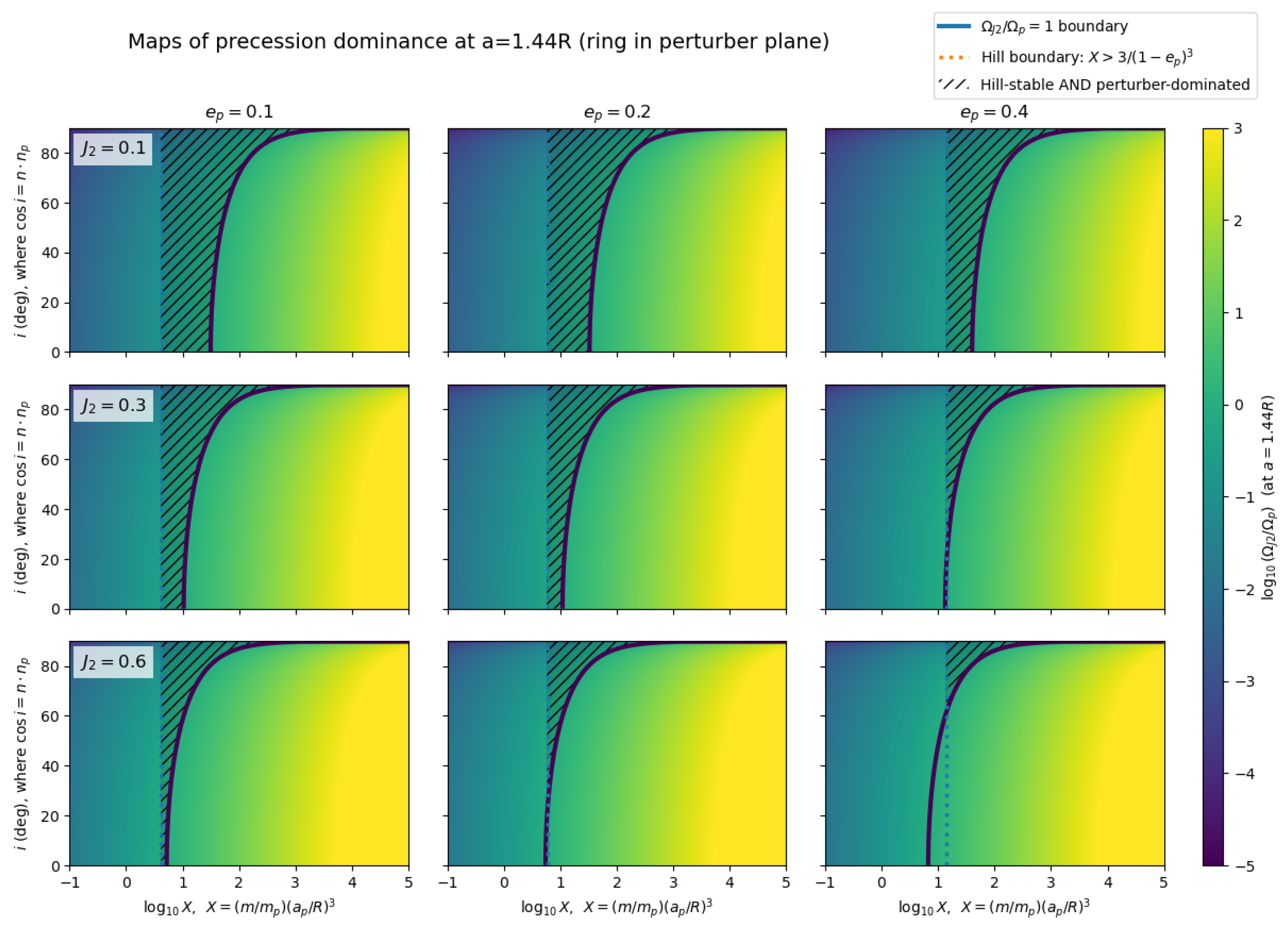
Now we explore if rings around minor bodies can be tilted as a result of the perturbation from a satellite. Parameters which satisfy the criteria in Equation (6) are in the shaded region of Figure 1. Colors encode the relative strength of oblateness and satellite perturbations, while lines denote the thresholds of stability and satellite perturbation dominance.

The second inequality of Equation (6) is trivially satisfied if the primary’s oblateness vanishes, i.e., $J_2=0$. However, although it is a useful simplification in many studies (see, e.g., [18]), it is obviously unphysical, especially for bodies which are highly non-spherical. For example, ref. [19] assumes $J_2\approx 0.13$ for Chariklo, the first minor body discovered to have a ring. Nevertheless, the region of parameters resulting in off-equatorial rings in Figure 1 becomes considerably wider as the oblateness decreases, as expected.

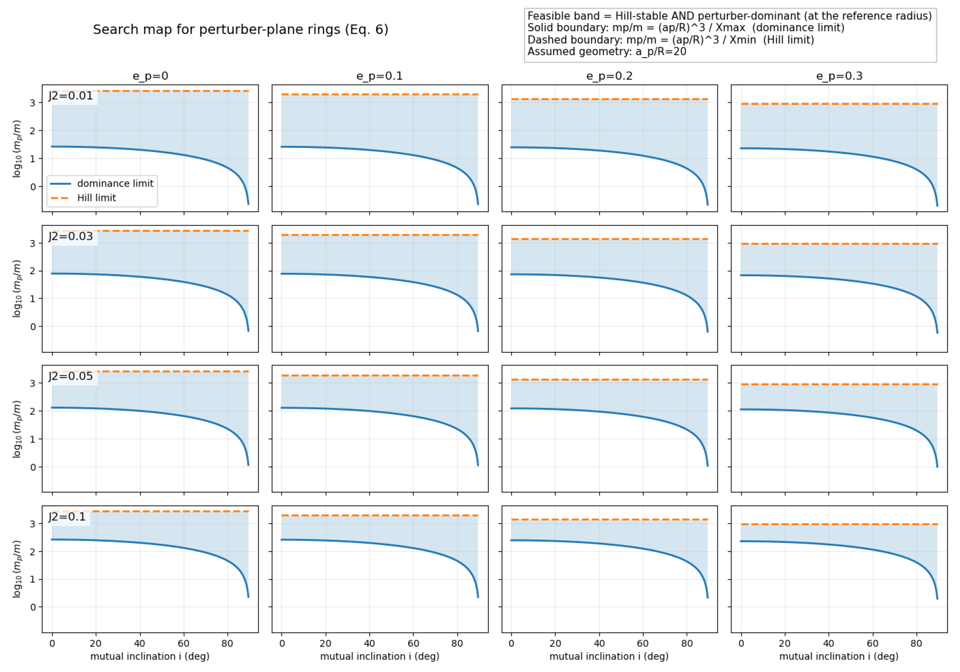
Inclination can also be crucial. Importantly, even in the complete absence of external perturbers, planetary oblateness alone can result in polar, i.e., off-equatorial orbits, as is reflected by the $1/cosi$ factor [20]. Indeed, $\mathbf{n}·\mathbf{L}=0$ results in $\dot{\mathbf{L}}=0$; see Equations (1) and (2). This is reflected by the widening of the shaded region in the panels of Figure 1 as higher inclinations are reached. It is further demonstrated in Figure 2, where the mass ratio is plotted against the inclination of the satellite. Note that we made a conservative assumption in deriving Equation (6), where we set ${\mathbf{n}}_{\mathrm{p}}·\widehat{\mathbf{L}}=1$. It may happen that the ring inclinations are governed by a satellite, yet its plane does not exactly fit that of the perturber. It means that off-equatorial rings may be more common than what is suggested in this work. However, one should take into account that if a ring is sufficiently inclined with respect to a distant perturber and eccentric, then it may be subject to destabilization via Kozai oscillations [21,22]. A more rigorous linear stability analysis, including the case of retrograde satellites (${\mathbf{n}}_{\mathrm{p}}·\widehat{\mathbf{L}}<0$), is left for future work.

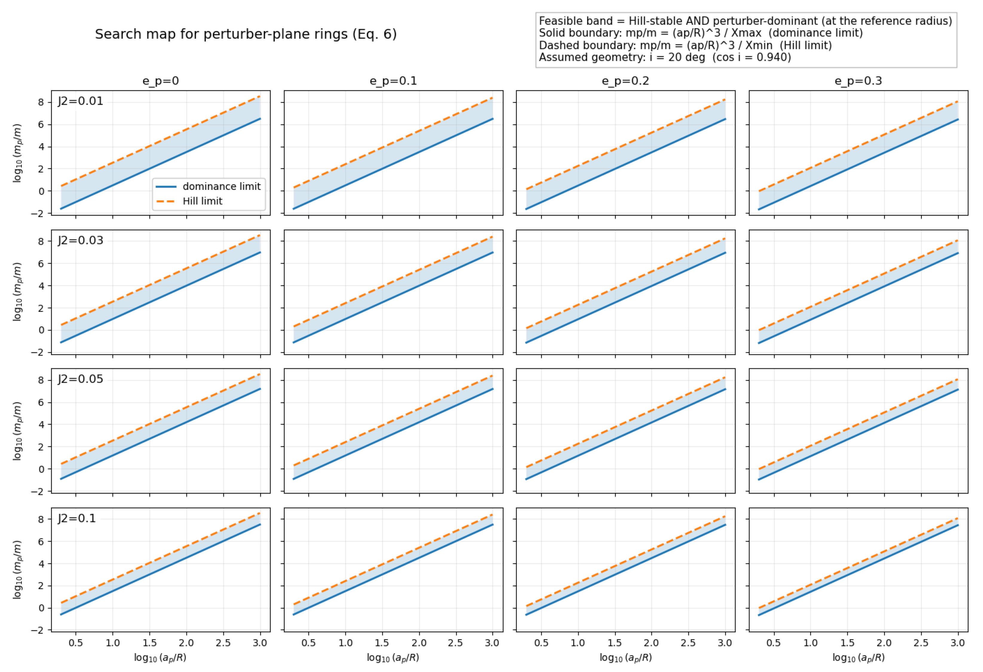
In order to have an off-equatorial ring, i.e., satisfying Equation (6), one needs to decrease $m/m_{\mathrm{p}}$ or $a_{\mathrm{p}}/R$, although only to the extent that Hill stability holds. This latter requirement breaks down easily with increasing eccentricity, as can be seen in the right panels of Figure 1. Also, for obvious reasons, the perturber’s semi-major axis cannot decrease below the primary’s radius. However, taking into account minor bodies in the solar system, there is no strict constraint for the masses and tilted rings can be possible in a variety of configurations, as shown in Figure 3. For example, binary minor planets have $m\sim m_{\mathrm{p}}$. However, $m\ll m_{\mathrm{p}}$ is also possible, as in the case of rings around moons, given they are sufficiently far away from their host planet. Ref. [23] investigates this configuration, although assuming $J_2=0$.

Although the oblateness has negligible effect on off-equatorial rings by assumption, it may influence the dynamics of the perturber. In particular, the condition ${\mathsf{\Omega }}_{J_2}\left(\mathrm{ring}\right)\ll {\mathsf{\Omega }}_{J_2}\left(\mathrm{perturber}\right)$, i.e., when we assume that oblateness perturbation on the perturber is much larger than that on the ring, translates to

$$\sqrt{m}{R}^{7/2}\ll \sqrt{m+m_{\mathrm{p}}}{a}_{\mathrm{p}}^{7/2}{(1-e_{\mathrm{p}}^2)}^2,$$

(7)

where in the formula of ${\mathsf{\Omega }}_{J_2}\left(\mathrm{perturber}\right)$, we made the substitution $m\to m+m_{\mathrm{p}}$. In this case, the orbital normal vector ${\mathbf{n}}_{\mathrm{p}}$ precesses with a rate that is related to the orbital frequency of the ring particles ($n=\sqrt{\mathcal{G}(m+m_{\mathrm{p}})a^3}$) as

$${\displaystyle \frac{{\mathsf{\Omega }}_{J_2}\left(\mathrm{perturber}\right)}{n}}\approx 0.868J_2{\left({\displaystyle \frac{R}{a_{\mathrm{p}}}}\right)}^{7/2}{\displaystyle \frac{cosi}{{(1-e_{\mathrm{p}}^2)}^2}},$$

(8)

which is small (given that the eccentricity is not too large due to Hill stability). Such a slow precession leaves the angle between $\mathsf{\Omega }$ and $\mathbf{L}$ (which is zero) adiabatically invariant, as shown heuristically in Appendix A. Physically, it means that the slowly precessing perturber drags the tilted plane with itself.

In conclusion, minor bodies may host rings which are significantly misaligned with respect to their equator as a result of a perturbing satellite. More precisely, the Laplace surface may considerably deviate from the equatorial plane within the Roche radius. Given the increasing number of such discoveries in the near future thanks to LSST [24], considering such configurations may be important in accurately modeling the dynamics of rings around minor bodies.

References

1. Sicardy, B. Dynamics of Planetary Rings. In Dynamics of Extended Celestial Bodies and Rings; Souchay, J., Ed.; Springer: Berlin/Heidelberg, Germany, 2006; Volume 682, p. 183. [Google Scholar] [CrossRef]
2. Goldreich, P.; Tremaine, S. The dynamics of planetary rings. Annu. Rev. Astron. Astrophys. 1982, 20, 249–283. [Google Scholar] [CrossRef]
3. Murray, C.D.; Dermott, S.F. Solar System Dynamics; Cambridge University Press: Cambridge, UK, 1999. [Google Scholar]
4. Braga-Ribas, F.; Sicardy, B.; Ortiz, J.L.; Snodgrass, C.; Roques, F.; Vieira-Martins, R.; Camargo, J.I.B.; Assafin, M.; Duffard, R.; Jehin, E.; et al. A ring system detected around the Centaur (10199) Chariklo. Nature 2014, 508, 72–75. [Google Scholar] [CrossRef] [PubMed]
5. Morgado, B.E.; Sicardy, B.; Braga-Ribas, F.; Desmars, J.; Gomes-Júnior, A.R.; Bérard, D.; Leiva, R.; Ortiz, J.L.; Vieira-Martins, R.; Benedetti-Rossi, G.; et al. Refined physical parameters for Chariklo’s body and rings from stellar occultations observed between 2013 and 2020. Astron. Astrophys. 2021, 652, A141. [Google Scholar] [CrossRef]
6. Ortiz, J.L.; Duffard, R.; Pinilla-Alonso, N.; Alvarez-Candal, A.; Santos-Sanz, P.; Morales, N.; Fernández-Valenzuela, E.; Licandro, J.; Campo Bagatin, A.; Thirouin, A. Possible ring material around centaur (2060) Chiron. Astron. Astrophys. 2015, 576, A18. [Google Scholar] [CrossRef]
7. Ruprecht, J.D.; Bosh, A.S.; Person, M.J.; Bianco, F.B.; Fulton, B.J.; Gulbis, A.A.S.; Bus, S.J.; Zangari, A.M. 29 November 2011 stellar occultation by 2060 Chiron: Symmetric jet-like features. Icarus 2015, 252, 271–276. [Google Scholar] [CrossRef]
8. Ortiz, J.L.; Santos-Sanz, P.; Sicardy, B.; Benedetti-Rossi, G.; Bérard, D.; Morales, N.; Duffard, R.; Braga-Ribas, F.; Hopp, U.; Ries, C.; et al. The size, shape, density and ring of the dwarf planet Haumea from a stellar occultation. Nature 2017, 550, 219–223. [Google Scholar] [CrossRef]
9. Morgado, B.E.; Sicardy, B.; Braga-Ribas, F.; Ortiz, J.L.; Salo, H.; Vachier, F.; Desmars, J.; Pereira, C.L.; Santos-Sanz, P.; Sfair, R.; et al. A dense ring of the trans-Neptunian object Quaoar outside its Roche limit. Nature 2023, 614, 239–243. [Google Scholar] [CrossRef]
10. Sicardy, B.; Leiva, R.; Renner, S.; Roques, F.; El Moutamid, M.; Santos-Sanz, P.; Desmars, J. Ring dynamics around non-axisymmetric bodies with application to Chariklo and Haumea. Nat. Astron. 2019, 3, 146–153. [Google Scholar] [CrossRef]
11. Merline, W.J.; Weidenschilling, S.J.; Durda, D.D.; Margot, J.L.; Pravec, P.; Storrs, A.D. Asteroids Do Have Satellites. In Asteroids III; Bottke, W.F., Jr., Cellino, A., Paolicchi, P., Binzel, R.P., Eds.; University of Arizona Press: Tucson, AZ, USA, 2002; pp. 289–312. [Google Scholar]
12. Richardson, D.C.; Walsh, K.J. Binary Minor Planets. Annu. Rev. Earth Planet. Sci. 2006, 34, 47–81. [Google Scholar] [CrossRef]
13. Nesvorný, D.; Youdin, A.N.; Richardson, D.C. Formation of Kuiper Belt Binaries by Gravitational Collapse. Astron. J. 2010, 140, 785–793. [Google Scholar] [CrossRef]
14. Milankovitch, M. Über die verwendung vektorieller bahnelemente in der störungsrechnung. Bull. Serb. Acad. Math. Nat. A 1939, 6, 1. [Google Scholar]
15. Tremaine, S.; Touma, J.; Namouni, F. Satellite Dynamics on the Laplace Surface. Astron. J. 2009, 137, 3706–3717. [Google Scholar] [CrossRef]
16. Grishin, E.; Perets, H.B.; Zenati, Y.; Michaely, E. Generalized Hill-stability criteria for hierarchical three-body systems at arbitrary inclinations. Mon. Not. R. Astron. Soc. 2017, 466, 276–285. [Google Scholar] [CrossRef]
17. Burns, J.A.; Cuzzi, J.N.; Durisen, R.H.; Hamill, P. On the ’thickness’ of Saturn’s rings caused by satellite and solar perturbations and by planetary precession. Astron. J. 1979, 84, 1783–1801. [Google Scholar] [CrossRef]
18. Regály, Z.; Fröhlich, V.; Kiss, C. Celestial sunflowers: Survival of rings around small planetary bodies under solar radiation pressure. Astron. Astrophys. 2025, 697, A116. [Google Scholar] [CrossRef]
19. Giuliatti Winter, S.M.; Madeira, G.; Ribeiro, T.; Winter, O.C.; Barbosa, G.O.; Borderes-Motta, G. The stability around Chariklo and the confinement of its rings. Astron. Astrophys. 2023, 679, A62. [Google Scholar] [CrossRef]
20. Dobrovolskis, A.R.; Borderies, N.J.; Steiman-Cameron, T.Y. Stability of polar rings around Neptune. Icarus 1989, 81, 132–144. [Google Scholar] [CrossRef]
21. Kozai, Y. Secular perturbations of asteroids with high inclination and eccentricity. Astron. J. 1962, 67, 591–598. [Google Scholar] [CrossRef]
22. Naoz, S. The Eccentric Kozai-Lidov Effect and Its Applications. Annu. Rev. Astron. Astrophys. 2016, 54, 441–489. [Google Scholar] [CrossRef]
23. Sucerquia, M.; Alvarado-Montes, J.A.; Zuluaga, J.I.; Cuello, N.; Cuadra, J.; Montesinos, M. The missing rings around Solar System moons. Astron. Astrophys. 2024, 691, A74. [Google Scholar] [CrossRef]
24. Ivezić, Ž.; Kahn, S.M.; Tyson, J.A.; Abel, B.; Acosta, E.; Allsman, R.; Alonso, D.; AlSayyad, Y.; Anderson, S.F.; Andrew, J.; et al. LSST: From Science Drivers to Reference Design and Anticipated Data Products. Astrophys. J. 2019, 873, 111. [Google Scholar] [CrossRef]
25. Nambu, Y. Generalized Hamiltonian Dynamics. Phys. Rev. D 1973, 7, 2405–2412. [Google Scholar] [CrossRef]
Figure 1. Heat map showing the relative strength of the primary’s oblateness (yellow) and a satellite’s perturbation (blue). The solid curve separates the regions where any of the two effects becomes dominant. The dotted line marks the boundary of Hill stability. Rings in the shaded region are tilted as the result of a satellite’s perturbation.
Universe 12 00108 g001
Figure 2. Allowed mass ratio and inclination parameters for off-equatorial rings by Equation (6). The solid and dashed curves have the same meaning as in Figure 1. The available parameter space is clearly wider for higher inclinations.
Universe 12 00108 g002
Figure 3. The same as Figure 2 but for semi-major axis instead of eccentriciy. Binary minor bodies lie in the lower left, while ringed moons around gas giants lie in the upper right part of the blue-shaded stripe.
Universe 12 00108 g003
Disclaimer/Publisher’s Note: The statements, opinions and data contained in all publications are solely those of the individual author(s) and contributor(s) and not of MDPI and/or the editor(s). MDPI and/or the editor(s) disclaim responsibility for any injury to people or property resulting from any ideas, methods, instructions or products referred to in the content.