
Effective Estimation of Dynamic Metabolic Fluxes Using 13C Labeling and Piecewise Affine Approximation: From Theory to Practical Applicability

Abstract
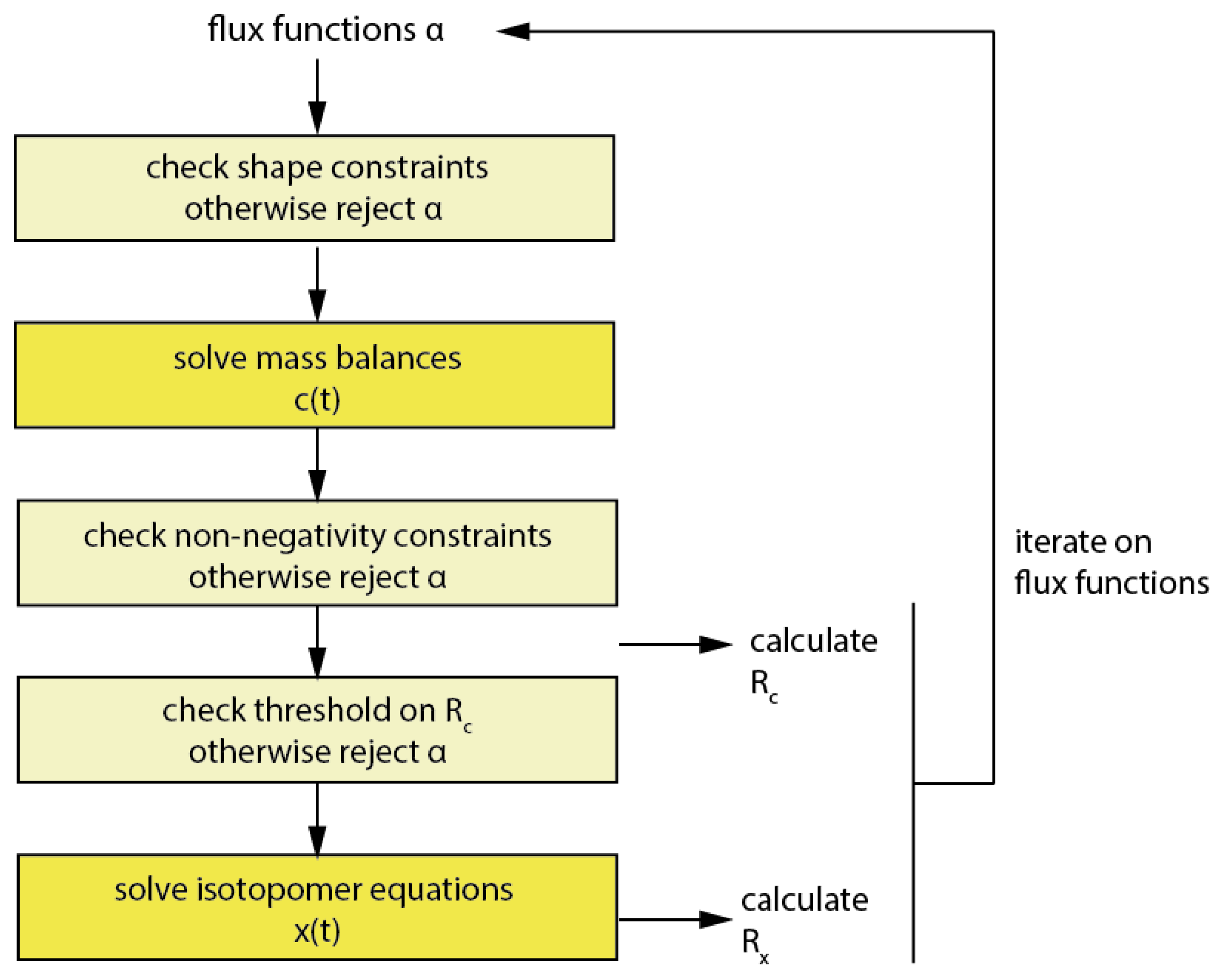
:
1. Introduction
- (1)
- Genetic adaption by mutagenesis and selection with a timescale of several generation times [3],
- (2)
- Adaption of gene expression levels with a timescale of minutes [4],
- (3)
- Post-translational modifications with a time constant on the order of seconds and
- (4)
- Kinetic response which is considered an inherent property of the enzymes in the metabolic network and therefore persistent.
- (1)
- (2)
- The kinetic functions have to be chosen a priori, which means that the mechanism of every enzyme and all interactions between metabolites and enzymes involved in the regarded metabolic network have to be selected before parameter optimization. Especially, the kinetic formats of each reaction in larger metabolic networks are yet unknown, unclear, or shall be deduced from the captured observables.
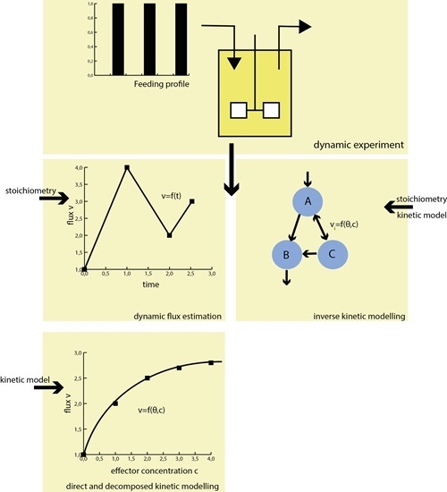
Experimental Requirements for in Vivo Dynamic Flux Estimation
- •
- A stimulus-response experiment should lead to perturbation(s) strong enough to cover a significant (metabolite) concentration space for good identification of the kinetic parameters [22].
- •
- The metabolomics should preferably have a complete coverage of the regarded intracellular metabolic response, e.g., intracellular concentrations, which moreover have to be quantitative.
- •
- (1)
- They generate repetitive concentration patterns in time, allowing for dense sampling from multiple cycles as well as application of 13C labeling from a single experiment.
- (2)
- The feast/famine perturbation includes both: the transient from limitation to excess as well as a return to limitation in a short timeframe of minutes.
- (3)
- In this setup, the starting metabolite concentrations of each cycle are the same as the endpoint, which means there is no net metabolite accumulation during one cycle (material is washed out with the biomass).
2. Results and Discussion
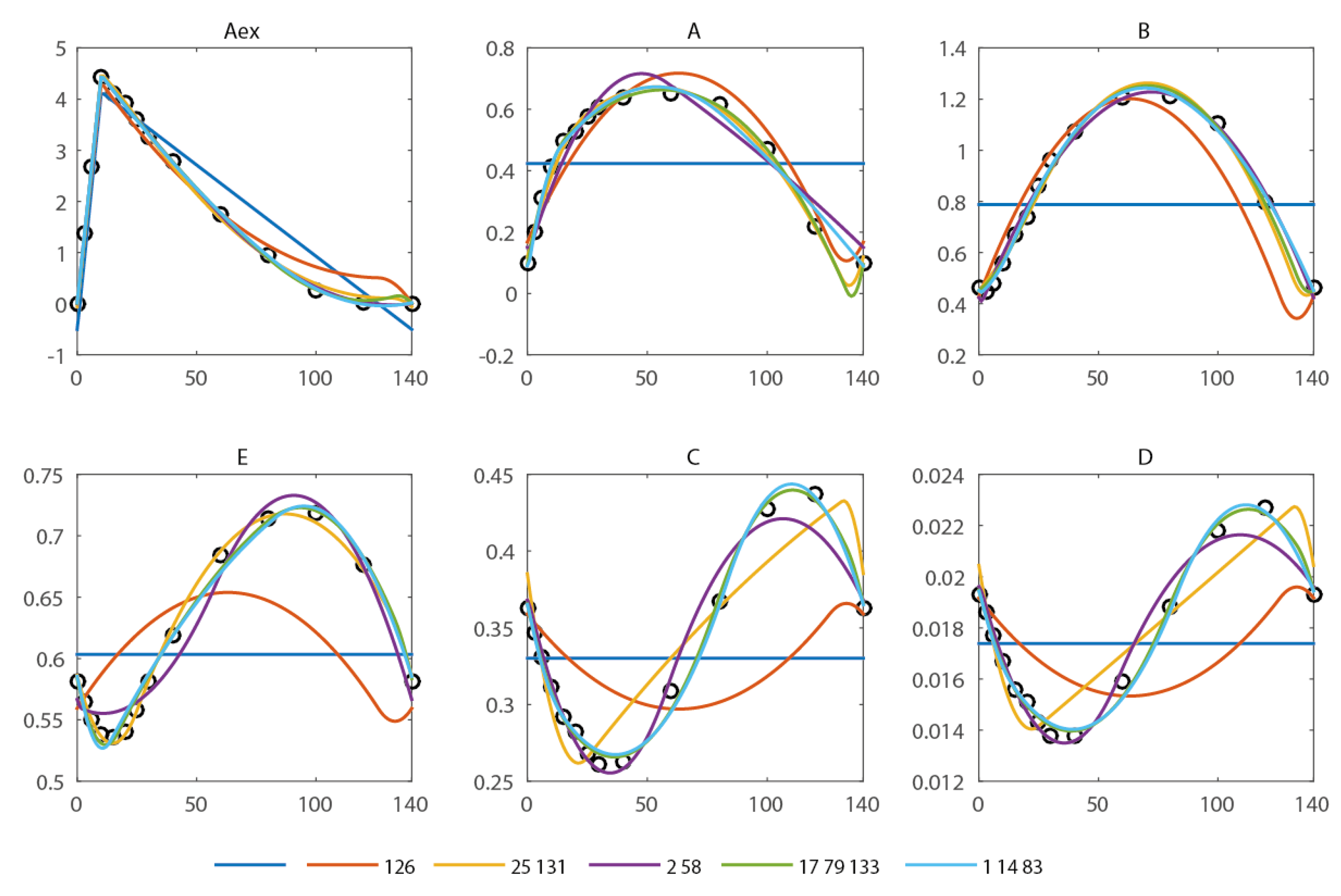
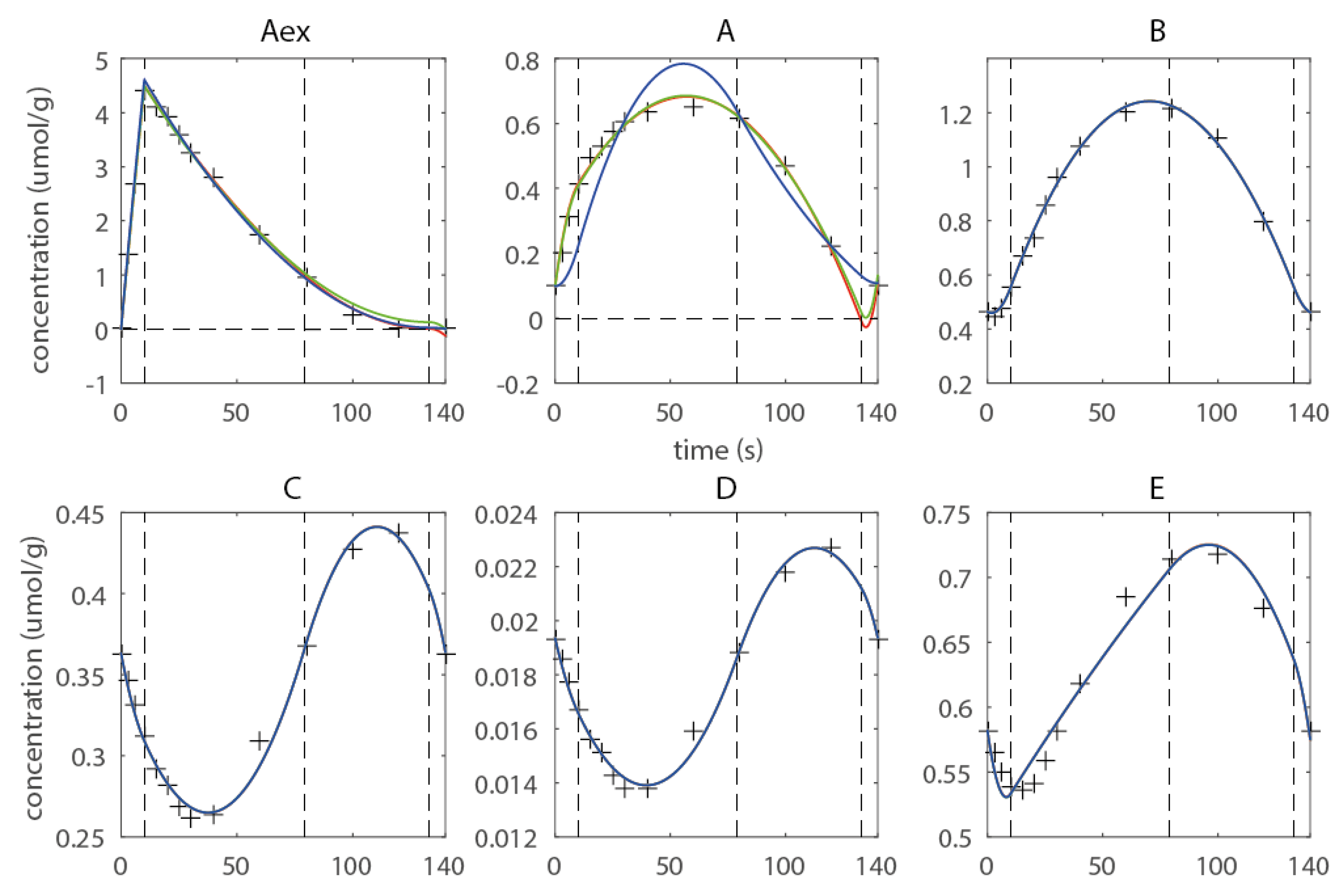
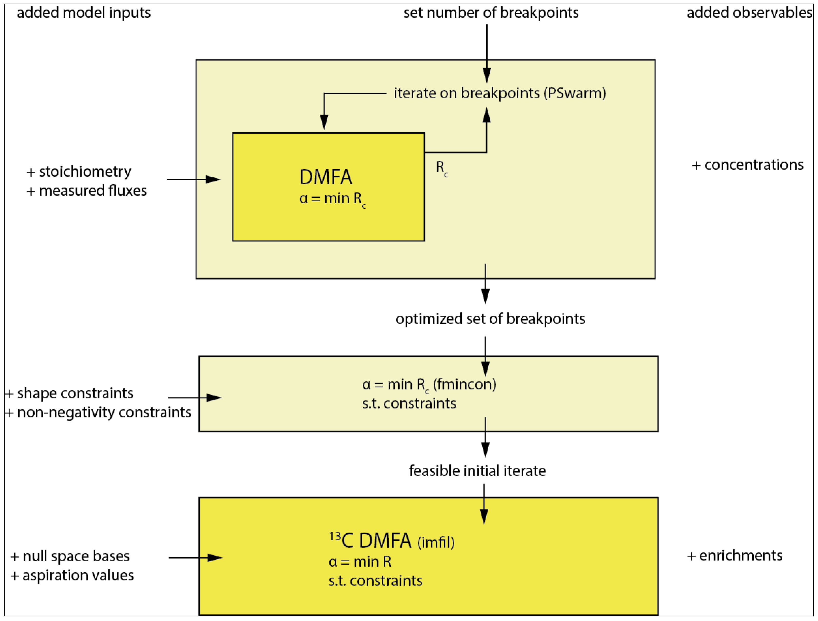
2.1. Computation of an Initial Set of Breakpoints Using the Concentration Measurements
- (1)
- The number of breakpoints and
- (2)
- The placement of breakpoints.


| Break Points (s) | #p | RSS | R2 | AIC | |
|---|---|---|---|---|---|
| - | 8 | 579.7 | - | - | 91.7 |
| 126 | 16 | 134.6 | 0.77 | 0.72 | 45.5 |
| 25, 131 | 24 | 15.1 | 0.97 | 0.97 | −31.6 |
| 2, 58 | 24 | 22.2 | 0.96 | 0.95 | −15.2 |
| 17, 79, 133 | 32 | 2.3 | 1.00 | 0.99 | −95.7 |
| 1, 14, 83 | 32 | 4.7 | 0.99 | 0.99 | −65.5 |
2.2. Introduction of Shape-Prescriptive Constraints

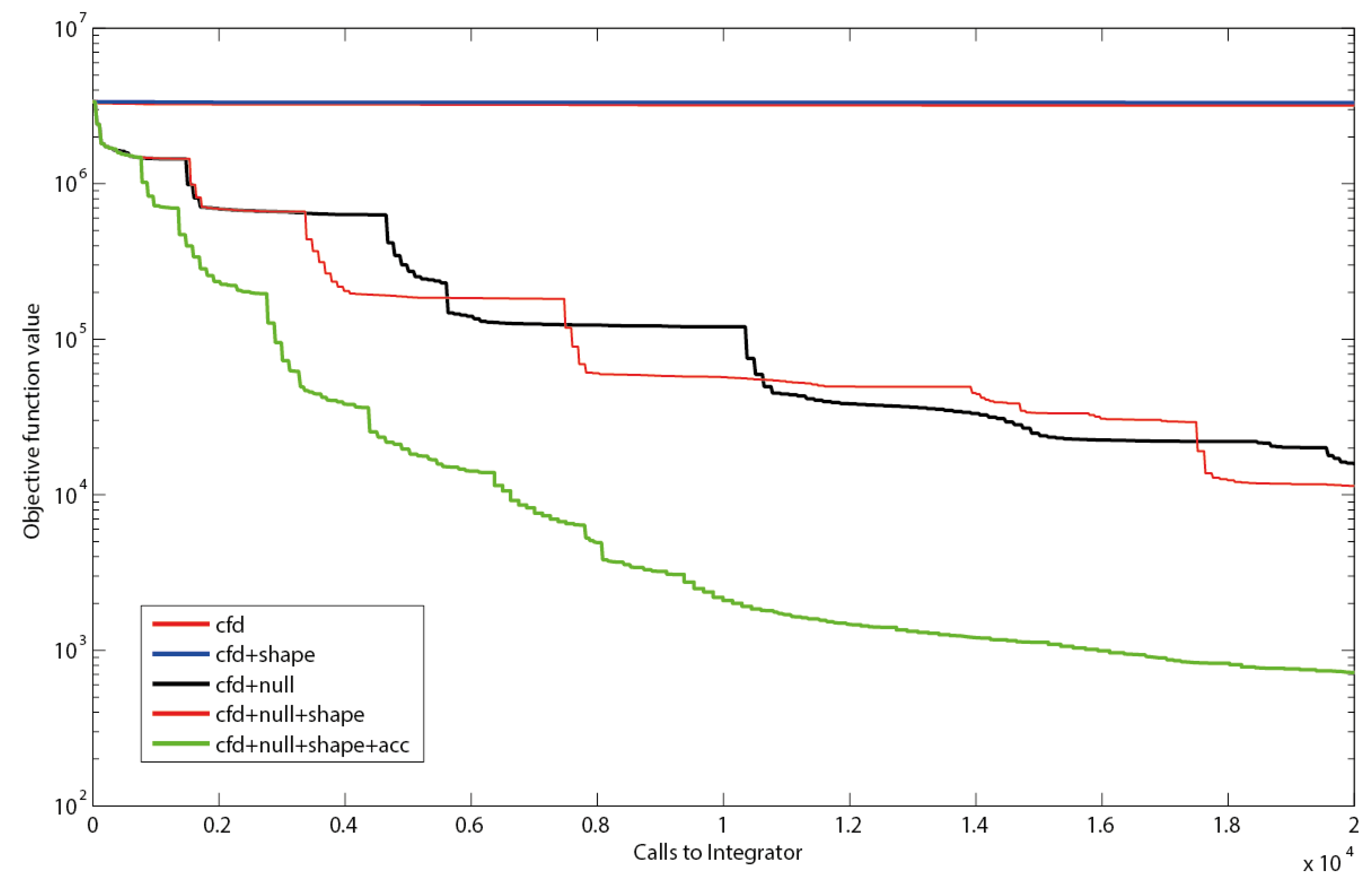
2.3. Estimating Flux Functions Using the Implicit Filtering Algorithm
3. Materials and Methods
3.1. Used Models and Data
3.2. Mathematical Modeling of Dynamic 13C Labeling Experiments Using PWA Flux Functions
3.3. Flux Functions and Nomenclature in the PWA Flux Framework
3.4. Balancing of Metabolites and Solution of the Metabolite Mass Balances
3.5. Sufficient Breakpoint Selection
3.6. Introducing Constraints
3.6.1. Specific Constraints for Feast-Famine Conditions
- (1)
- In a stable feast-famine regime the metabolite concentration at the end of one cycle has the same concentration as in the beginning (of the next cycle).
- (2)
- Similarly, the flux at the end of the feast famine cycle has to be the same as in the beginning. Otherwise no stable, repetitive cycles were obtained.
3.6.2. Non-Negativity Constraints
3.6.3. General Shape-Prescriptive Constraints
3.6.4. Monotonicity and Convexity Constraints
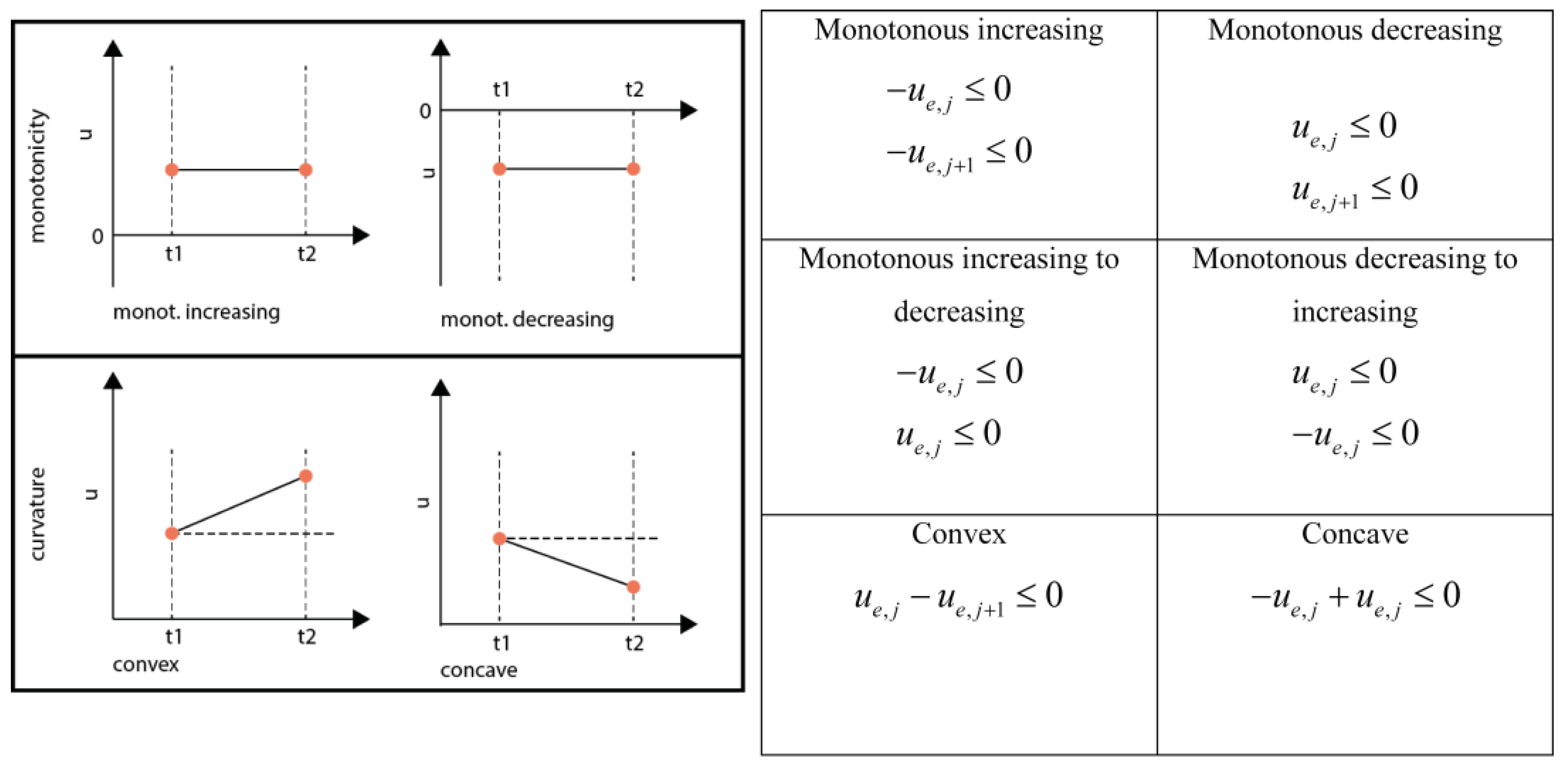
3.6.5. Equality Shape Constraints
3.7. 13C DMFA
3.7.1. The Implicit Filtering (Imfil) Optimization Algorithm
3.7.2. Implementation of the Constraints in Implicit Filtering (Imfil)
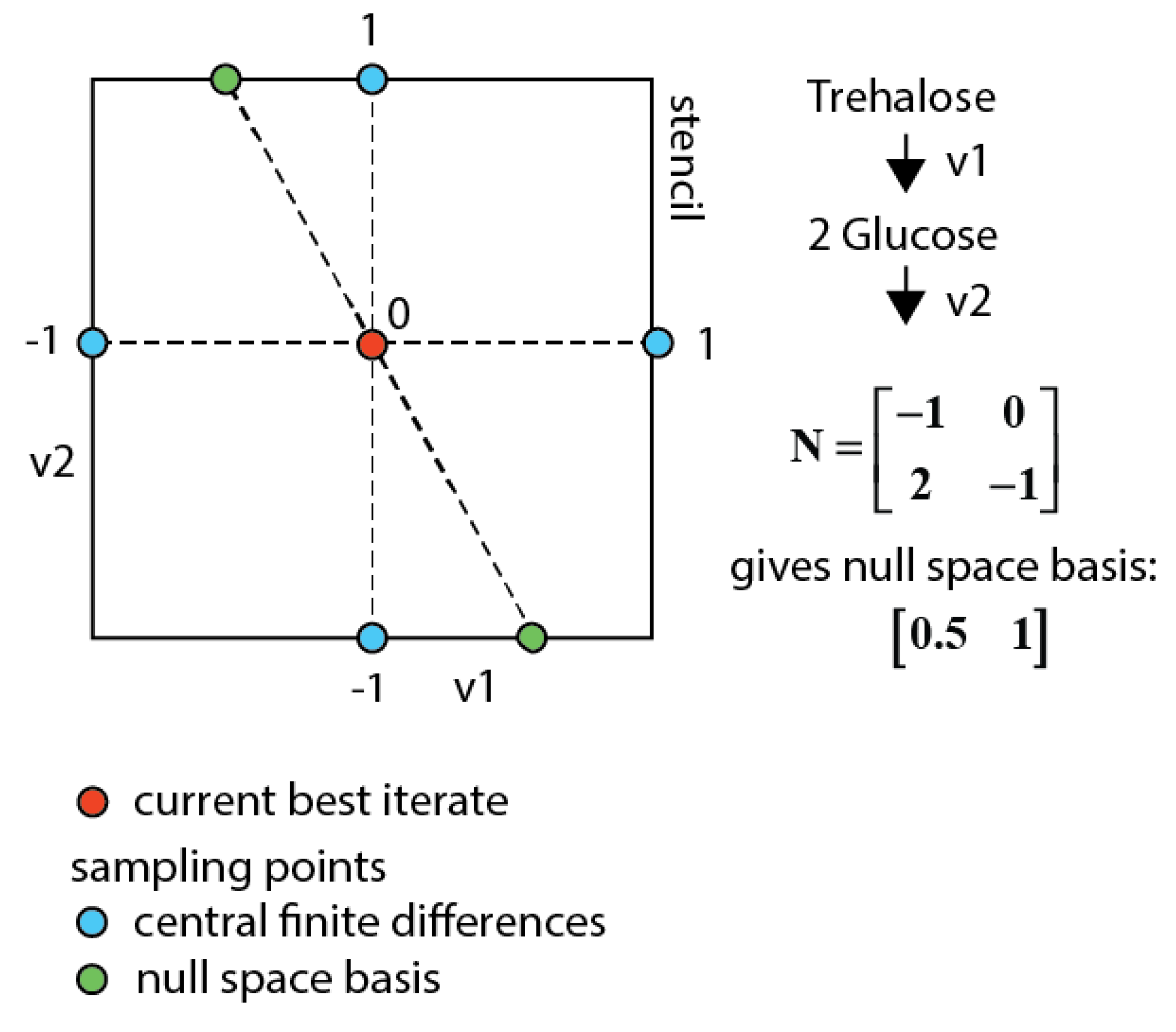
3.7.3. Null-Space-Based Sampling

4. Conclusions
Supplementary Materials
Acknowledgments
Author Contributions
Conflicts of Interest
Symbols and Abbreviations
| Subscript | |
| 0 | Initial condition |
| asp | Aspiration value |
| e | Metabolite identifier |
| end | End of feast famine cycle |
| i | index of flux |
| j | index of breakpoint |
| k | index of domain |
| m | Index of measurement |
| M | All measurements |
| Superscript | |
| inp | Enrichment of used substrate for labelling |
| b | Known flux |
| n | Unknown flux |
| f | Number of unknown fluxes |
| General | |
| a | Scaling factor |
| e | Enzyme activity |
| R, RSS | (weighted) residual sum of squares |
| R2 | Coefficient of determination |
| θ | Flux function parameters |
| α | Kinetic parameters |
| c | (metabolite) concentration |
| x | (C-molar) enrichment |
| v | Flux |
| u | Right-hand-side (dc/dt) |
| W | Weight matrix |
| ^ | Optimal estimate |
| t | Time |
| λ | Lagrange multiplier |
| w | Translation vector of the null space |
| N | Stoichiometry matrix |
| σ | Standard deviation |
| imfil | Implicit filtering algorithm |
| PWA | Piecewise affine |
| acc | Accelerator for imfil |
| DMFA | Dynamic metabolic flux analysis |
| AIC | Aikaike information criterion |
References
- Postma, P.W.; Lengeler, J.W.; Jacobson, G.R. Phosphoenolpyruvate:Carbohydrate phosphotransferase systems of bacteria. Microbiol. Rev. 1993, 57, 543–594. [Google Scholar] [PubMed]
- Lapin, A.; Klann, M.; Reuss, M. Multi-scale spatio-temporal modeling: Lifelines of microorganisms in bioreactors and tracking molecules in cells. In Biosystems Engineering II; Wittmann, C., Krull, R., Eds.; Springer: Berlin, Germany; Heidelberg, Germany, 2010; Volume 121, pp. 23–43. [Google Scholar]
- Herring, C.D.; Raghunathan, A.; Honisch, C.; Patel, T.; Applebee, M.K.; Joyce, A.R.; Albert, T.J.; Blattner, F.R.; van den Boom, D.; Cantor, C.R.; et al. Comparative genome sequencing of escherichia coli allows observation of bacterial evolution on a laboratory timescale. Nat. Genet. 2006, 38, 1406–1412. [Google Scholar] [CrossRef] [PubMed]
- Kresnowati, M.T.; van Winden, W.A.; Almering, M.J.; ten Pierick, A.; Ras, C.; Knijnenburg, T.A.; Daran-Lapujade, P.; Pronk, J.T.; Heijnen, J.J.; Daran, J.M. When transcriptome meets metabolome: Fast cellular responses of yeast to sudden relief of glucose limitation. Mol. Syst. Biol. 2006, 2, 49. [Google Scholar] [CrossRef] [PubMed]
- Teusink, B.; Passarge, J.; Reijenga, C.A.; Esgalhado, E.; van der Weijden, C.C.; Schepper, M.; Walsh, M.C.; Bakker, B.M.; van Dam, K.; Westerhoff, H.V.; et al. Can yeast glycolysis be understood in terms of in vitro kinetics of the constituent enzymes? Testing biochemistry. Eur. J. Biochem./FEBS 2000, 267, 5313–5329. [Google Scholar] [CrossRef]
- Theobald, U.; Baltes, M.; Rizzi, M.; Reuss, M. Structured metabolic modelling applied to dynamic simulation of the crabtree-and pasteur-effect in baker’s yeast. In Biochemical Engineering-Stuttgart; Vch Pub: Weinheim, NY, USA, 1991; pp. 361–364. [Google Scholar]
- Heijnen, J.J. Approximative kinetic formats used in metabolic network modeling. Biotechnol. Bioeng. 2005, 91, 534–545. [Google Scholar] [CrossRef] [PubMed]
- Jia, G.; Stephanopoulos, G.; Gunawan, R. Incremental parameter estimation of kinetic metabolic network models. BMC Syst. Biol. 2012, 6, 142. [Google Scholar] [CrossRef] [PubMed]
- Chou, I.-C.; Martens, H.; Voit, E. Parameter estimation in biochemical systems models with alternating regression. Theor. Biol. Med. Model. 2006, 3, 25. [Google Scholar] [CrossRef] [PubMed]
- Wahl, S.A.; Haunschild, M.D.; Oldiges, M.; Wiechert, W. Unravelling the regulatory structure of biochemical networks using stimulus response experiments and large-scale model selection. IEE Proc. Syst. Biol. 2006, 153, 275–285. [Google Scholar] [CrossRef]
- Tran, L.M.; Rizk, M.L.; Liao, J.C. Ensemble modeling of metabolic networks. Biophys. J. 2008, 95, 5606–5617. [Google Scholar] [CrossRef] [PubMed]
- Link, H.; Kochanowski, K.; Sauer, U. Systematic identification of allosteric protein-metabolite interactions that control enzyme activity in vivo. Nat. Biotechnol. 2013, 31, 357–361. [Google Scholar] [CrossRef] [PubMed]
- Jia, G.; Stephanopoulos, G.; Gunawan, R. Ensemble kinetic modeling of metabolic networks from dynamic metabolic profiles. Metabolites 2012, 2, 891–912. [Google Scholar] [CrossRef] [PubMed]
- Goel, G.; Chou, I.C.; Voit, E.O. System estimation from metabolic time-series data. Bioinformatics 2008, 24, 2505–2511. [Google Scholar] [CrossRef] [PubMed]
- Liu, Y.; Gunawan, R. Parameter estimation of dynamic biological network models using integrated fluxes. BMC Syst. Biol. 2014, 8, 127. [Google Scholar] [CrossRef] [PubMed]
- Abate, A.; Hillen, R.C.; Aljoscha Wahl, S. Piecewise affine approximations of fluxes and enzyme kinetics from in vivo 13c labeling experiments. Int. J. Robust Nonlinear Control 2012, 22, 1120–1139. [Google Scholar] [CrossRef]
- De Jonge, L.; Buijs, N.A.A.; Heijnen, J.J.; van Gulik, W.M.; Abate, A.; Wahl, S.A. Flux response of glycolysis and storage metabolism during rapid feast/famine conditions in penicillium chrysogenum using dynamic 13c labeling. Biotechnol. J. 2014, 9, 372–385. [Google Scholar] [CrossRef] [PubMed]
- Leighty, R.W.; Antoniewicz, M.R. Dynamic metabolic flux analysis (dmfa): A framework for determining fluxes at metabolic non-steady state. Metab. Eng. 2011, 13, 745–755. [Google Scholar] [CrossRef] [PubMed]
- Bonarius, H.P.J.; Schmid, G.; Tramper, J. Flux analysis of underdetermined metabolic networks: The quest for the missing constraints. Trends Biotechnol. 1997, 15, 308–314. [Google Scholar] [CrossRef]
- Raue, A.; Kreutz, C.; Maiwald, T.; Bachmann, J.; Schilling, M.; Klingmuller, U.; Timmer, J. Structural and practical identifiability analysis of partially observed dynamical models by exploiting the profile likelihood. Bioinformatics 2009, 25, 1923–1929. [Google Scholar] [CrossRef] [PubMed]
- Isermann, N.; Wiechert, W. Metabolic isotopomer labeling systems. Part ii: Structural flux identifiability analysis. Math. Biosci. 2003, 183, 175–214. [Google Scholar] [CrossRef]
- Degenring, D.; Froemel, C.; Dikta, G.; Takors, R. Sensitivity analysis for the reduction of complex metabolism models. J. Process Control 2004, 14, 729–745. [Google Scholar] [CrossRef]
- Wiechert, W.; Möllney, M.; Petersen, S.; de Graaf, A.A. A universal framework for 13C metabolic flux analysis. Metab. Eng. 2001, 3, 265–283. [Google Scholar] [CrossRef] [PubMed]
- Wu, L.; Mashego, M.R.; van Dam, J.C.; Proell, A.M.; Vinke, J.L.; Ras, C.; van Winden, W.A.; van Gulik, W.M.; Heijnen, J.J. Quantitative analysis of the microbial metabolome by isotope dilution mass spectrometry using uniformly 13c-labeled cell extracts as internal standards. Anal. Biochem. 2005, 336, 164–171. [Google Scholar] [CrossRef] [PubMed]
- Van Kleeff, B.H.A.; Kuenen, J.G.; Heijnen, J.J. Heat flux measurements for the fast monitoring of dynamic responses to glucose additions by yeasts that were subjected to different feeding regimes in continuous culture. Biotechnol. Prog. 1996, 12, 510–518. [Google Scholar] [CrossRef] [PubMed]
- Suarez-Mendez, C.; Sousa, A.; Heijnen, J.; Wahl, A. Fast “feast/famine” cycles for studying microbial physiology under dynamic conditions: A case study with saccharomyces cerevisiae. Metabolites 2014, 4, 347. [Google Scholar] [CrossRef] [PubMed]
- Lange, H.C.; Eman, M.; van Zuijlen, G.; Visser, D.; van Dam, J.C.; Frank, J.; de Teixeira Mattos, M.J.; Heijnen, J.J. Improved rapid sampling for in vivo kinetics of intracellular metabolites in saccharomyces cerevisiae. Biotechnol. Bioeng. 2001, 75, 406–415. [Google Scholar] [CrossRef] [PubMed]
- Van Heerden, J.H.; Wortel, M.T.; Bruggeman, F.J.; Heijnen, J.J.; Bollen, Y.J.M.; Planqué, R.; Hulshof, J.; O’Toole, T.G.; Wahl, S.A.; Teusink, B. Lost in transition: Startup of glycolysis yields subpopulations of nongrowing cells. Science 2014, 343. [Google Scholar] [CrossRef] [PubMed]
- Antoniewicz, M.R.; Kelleher, J.K.; Stephanopoulos, G. Elementary metabolite units (emu): A novel framework for modeling isotopic distributions. Metab. Eng. 2007, 9, 68–86. [Google Scholar] [CrossRef] [PubMed]
- Klamt, S.; Schuster, S.; Gilles, E.D. Calculability analysis in underdetermined metabolic networks illustrated by a model of the central metabolism in purple nonsulfur bacteria. Biotechnol. Bioeng. 2002, 77, 734–751. [Google Scholar] [CrossRef] [PubMed]
- Vaz, A.I.F.; Vicente, L.N. A particle swarm pattern search method for bound constrained global optimization. J. Glob. Optim. 2007, 39, 197–219. [Google Scholar] [CrossRef]
- Akaike, H. A new look at the statistical model identification. In Selected Papers of Hirotugu akaike; Parzen, E., Tanabe, K., Kitagawa, G., Eds.; Springer: New York, NY, USA, 1998; pp. 215–222. [Google Scholar]
- Montgomery, D.C.; Runger, G.C. Applied Statistics and Probability for Engineers; John Wiley & Sons: Hoboken, NJ, USA, 2010. [Google Scholar]
- Kelley, C.T. Implicit Filtering; Society for Industrial and Applied Mathematics: Philadelphia, PA, USA, 2011. [Google Scholar]
© 2015 by the authors; licensee MDPI, Basel, Switzerland. This article is an open access article distributed under the terms and conditions of the Creative Commons Attribution license (http://creativecommons.org/licenses/by/4.0/).
Share and Cite
Schumacher, R.; Wahl, S.A. Effective Estimation of Dynamic Metabolic Fluxes Using 13C Labeling and Piecewise Affine Approximation: From Theory to Practical Applicability. Metabolites 2015, 5, 697-719. https://doi.org/10.3390/metabo5040697
Schumacher R, Wahl SA. Effective Estimation of Dynamic Metabolic Fluxes Using 13C Labeling and Piecewise Affine Approximation: From Theory to Practical Applicability. Metabolites. 2015; 5(4):697-719. https://doi.org/10.3390/metabo5040697
Chicago/Turabian StyleSchumacher, Robin, and S. Aljoscha Wahl. 2015. "Effective Estimation of Dynamic Metabolic Fluxes Using 13C Labeling and Piecewise Affine Approximation: From Theory to Practical Applicability" Metabolites 5, no. 4: 697-719. https://doi.org/10.3390/metabo5040697
APA StyleSchumacher, R., & Wahl, S. A. (2015). Effective Estimation of Dynamic Metabolic Fluxes Using 13C Labeling and Piecewise Affine Approximation: From Theory to Practical Applicability. Metabolites, 5(4), 697-719. https://doi.org/10.3390/metabo5040697